Learning to search efficiently for causally near-optimal treatments
Abstract
Finding an effective medical treatment often requires a search by trial and error. Making this search more efficient by minimizing the number of unnecessary trials could lower both costs and patient suffering. We formalize this problem as learning a policy for finding a near-optimal treatment in a minimum number of trials using a causal inference framework. We give a model-based dynamic programming algorithm which learns from observational data while being robust to unmeasured confounding. To reduce time complexity, we suggest a greedy algorithm which bounds the near-optimality constraint. The methods are evaluated on synthetic and real-world healthcare data and compared to model-free reinforcement learning. We find that our methods compare favorably to the model-free baseline while offering a more transparent trade-off between search time and treatment efficacy.
1 Introduction
Finding a good treatment for a patient often involves trying out different options before a satisfactory one is found (Murphy et al. 2007). If the first-line drug is ineffective or has severe side-effects, guidelines may suggest it is replaced by or combined with another drug (Singh et al. 2016). These steps are repeated until an effective combination of drugs is found or all options are exhausted, a process which may span several years (NCCMH 2010). A long search adds to patient suffering and postpones potential relief. It is therefore critical that this process is made as time-efficient as possible.
We formalize the search for effective treatments as a policy optimization problem in an unknown decision process with finite horizon (Garcia and Ndiaye 1998). This has applications also outside of medicine: For example, in recommendation systems, we may sequentially propose new products or services to users with the hope of finding one that the user is interested in. Our goal is to perform as few trials as possible until the probability that there are untried actions which are significantly better is small—i.e., a near-optimal action has been found with high probability. Historical observations allow us to transfer knowledge and perform this search more efficiently for new subjects. As more actions are tried and their outcomes observed, our certainty about the lack of better alternatives increases. Importantly, even a failed trial may provide information that can guide the search policy.
In this work, we restrict our attention to actions whose outcomes are stationary in time. This implies both that repeated trials of the same action have the same outcome and that past actions do not causally impact the outcome of future actions. The stationarity assumption is justified, for example, for medical conditions where treatments manage symptoms but do not alter the disease state itself, or where the impact of sequential treatments is known to be additive. In such settings, past actions and outcomes may help predict the outcomes of future actions without having a causal effect on them.
We formalize learning to search efficiently for causally effective treatments as off-policy optimization of a policy which finds a near-optimal action for new contexts after as few trials as possible. Our setting differs from those typical of reinforcement or bandit learning (Sutton et al. 1998): (i) Solving the problem relies on transfer of knowledge from observational data. (ii) The stopping (near-optimality) criterion depends on a model of unobserved quantities. (iii) The number of trials in a single sequence is bounded by the number of available actions. We address identification of an optimal policy using a causal framework, accounting for potential confounding. We give a dynamic programming algorithm which learns policies that satisfy a transparent constraint on near-optimality for a given level of confidence, and a greedy approximation which satisfies a bound on this constraint. We show that greedy policies are sub-optimal in general, but that there are settings where they return policies with informative guarantees. In experiments, including an application derived from antibiotic resistance tests, our algorithms successfully learn efficient search policies and perform favorably to baselines.
2 Related work
Our problem is related to the bandit literature, which studies the search for optimal actions through trial and error (Lattimore and Szepesvári 2020), and in particular to contextual bandits (Abe et al. 2003; Chu et al. 2011). In our setting, a very small number of actions is evaluated, with the goal of terminating search as early as possible. This is closely related to the fixed-confidence variant of best-arm identification (Lattimore and Szepesvári 2020, Chapter 33.2), in which only exploration is performed. To solve this problem without trying each action at least once, we rely on transferring knowledge from previous trials. This falls within the scope of transfer and meta learning. Liao et al. 2020 explicitly tackled pooling knowledge across patients data to determine an optimal treatment policy in an RL setting and Maes et al. 2012 devised methods for meta-learning of exploration policies for contextual bandits. A notable difference is that we assume that outcomes of actions are stationary in time. We leverage this both in model identification and policy optimization.
Experiments continue to be the gold standard for evaluating adaptive treatment strategies (Nahum-Shani et al. 2012). However, these are not always feasible due to ethical or practical constraints. We approach our problem as causal estimation from observational data (Rosenbaum et al. 2010; Robins et al. 2000), or equivalently, as off-policy policy optimization and evaluation (Precup 2000; Kallus and Santacatterina 2018). Unlike many works, we do not fully rely on ignorability—that all confounders are measured and may be adjusted for. Zhang and Bareinboim 2019 recently studied the non-ignorable setting but allowed for limited online exploration. In this work we aim to bound the effect of unmeasured confounding rather than to eliminate it using experimental evidence.
Our problem is closely related to active learning (Lewis and Gale 1994), which has been used to develop testing policies that minimize the expected number of tests performed before an underlying hypothesis is identified. For a known distribution of hypotheses, finding an optimal policy is NP-hard (Chakaravarthy et al. 2007), but there exists greedy algorithms with approximation guarantees (Golovin et al. 2010). In our case, (i) the distribution is unknown, and (ii) hypotheses (outcomes) are only partially observed. Our problem is also related to optimal stopping (Jacka 1991) of processes but differs in that the process is controlled by our decision-making agent.
3 Learning to search efficiently for causally near-optimal treatments
We consider learning policies that search over a set of actions to find an action such that its outcome is near-optimal. When such an action is found, the search should be terminated as early as possible using a special stop action, denoted . Throughout, a high outcome is assumed to be preferred and we often refer to actions as “treatments”. The potential outcome may vary between subjects (contexts) depending on baseline covariates and unobserved factors. When a search starts, all potential outcomes are unobserved, but are successively revealed as more actions are tried, see the illustration in Figure 1. To guide selection of the next action, we learn from observational data of previous subjects.
Historical searches are observed through covariates and a sequence of action-outcome pairs . Note the distinction between interventional and observational outcomes; represents the potential outcome of performing action at time (Rubin 2005). We assume that are discrete, although our results may be generalized to the continuous case. Sequences of random variables are denoted with a bar and subscript, , and denotes the history up-to time , with . With slight abuse of notation, means that was used in and that it had the outcome . denotes the number of trials in . The set of histories of at most actions is denoted . Termination of a sequence is indicated by the sequence length and may either be the result of finding a satisfactory treatment or due to censoring. Hence, the full set of potential outcomes is not observed for most subjects. Observations are distributed according to .
We optimize a deterministic policy which suggests an action following observed history , starting with , or terminates the sequence. Formally, . Taking the action at a time point implies that . Let be the distribution in which actions are drawn according to the policy . For a given slack parameter and a confidence parameter , we wish to solve the following problem.
| (1) | ||||||
In (1), the objective equals the expected search length under and the constraint enforces that termination occurs only when there is low probability that a better action will be found among the unused alternatives. Note that if is known and is in , the constraint is automatically satisfied at . To evaluate the constraint, we need a model of unobserved potential outcomes. This is dealt with in Section 4. We address optimization of (1) for a known model in Section 5.
4 Causal identification and estimation of optimality conditions
Our assumed causal model for observed data is illustrated graphically in Figure 2(a). Most notably, the graph defines the causal structure between actions and outcomes—previous actions and outcomes are assumed to have no direct causal effect on future outcomes . To allow for correlations between outcomes, we posit the existence of counfounders (observed) and (unobserved) and an unobserved moderator . All other variables are assumed exogenous.
To evaluate the near-optimality constraint and solve (1), we must identify the probability
| (2) |
with the convention that if . Henceforth, let denote the set of untried actions at and let be all permutations of the elements in .
We state assumptions sufficient for identification of below. Throughout this work we assume that consistency, stationarity of outcomes and positivity always hold, and provide identifiability results both when ignorability holds (Section 4.1) and when it is violated (Section 4.2).
Identifying assumptions.
Define . Under the observational distribution , and evaluation distribution , for all , , and , we assume
- 1.
Consistency:
- 2.
Stationarity:
- 3.
Positivity:
- 4.
Ignorability:
Ignorability follows from the backdoor criterion applied to the causal model of Figure 2(a) when is empty (Pearl 2009). We expand on this setting next. In contrast to conventions typically used in the literature, positivity is specified w.r.t. the considered policy class. This ensures that every action could be observed at some point after every history that is possible under policies in . Under Assumption 2 (stationarity), there is no need to try the same treatment twice, since the outcome is already determined by the first trial. We can restrict our attention to non-repeating policies,
Non-repeating policies such as these take the form of a decision tree of depth at most .
Remark 1 (Assumptions 1–4 in practice).
Only the positivity assumption may be verified empirically; stationarity, consistency and ignorability must be justified by domain knowledge. Readers experienced with causal estimation will be familiar with the process of establishing ignorability and consistency through graphical arguments or reasoning about statistical independences. Stationarity is more specific to our setting and without it, the notion of a near-optimal action is not well-defined—the best action could change with time. This phenomenon occurs is settings where outcomes naturally increase or decrease over time, irrespective of interventions. For example, the cognitive function of patients with Alzheimer’s disease tends to decrease steadily over time (Arevalo-Rodriguez et al. 2015). As a result, measures of cognitive function for patients on a medication will be different depending on the stage of progression that the patient is in. As a rule-of-thumb, stationarity is better justified over small time-frames or for more stable conditions.
4.1 Identification without unmeasured confounders
Our stopping criterion is an interventional quantity which represents the probability that an unused action would be preferable to previously tried ones. In general, this is not equal to the rate at which such an action was preferable in observed data. Nevertheless, we prove that is identifiable from observational data in the case that does not exist (ignorability holds w.r.t. ). First, the following lemma shows that the order of history does not influence the probability of future outcomes.
Lemma 1.
Let be a permutation of . Under stationarity, for all and ,
| (3) |
Lemma 1 is proven in Appendix A.1. As a consequence, we may treat two histories with the same events in different order as equivalent when estimating .
We can now state the following result about identification of the near-optimality constraint of (1).
Theorem 1.
Under Assumptions 1–4, the stopping criterion in (2) is identifiable from the observational distribution . For any time step with history , let be an arbitrary permutation of . Then, for any sequence of untried actions with the (hypothetical) continued history at time corresponding to and , and with ,
| (4) |
A proof of Theorem 1 is given in Appendix A.2. Equation (4) gives a concrete means to estimate from observational data by constructing a model of . Due to Assumption 2 (stationarity), this model can be invariant to permutations of . Another important consequence of this result is that, because Theorem 1 holds for any future sequence of actions, (4) holds also over any convex combination for different future action sequences, such as the expectation over the empirical distribution. Using likely sequences under the behavior policy will lead to lower-variance estimates.
Remark 2.
In the fully discrete case, we may estimate using a probability table, and we do so in some experiments in Section 6. However, this becomes increasingly difficult for both statistical and computational reasons when and grow larger or when any of the variables are continuous. The permutation invariance given by Theorem 1 provides some relief but, nevertheless, the number of possible combinations (histories) grows exponentially with the number of actions. As a result, it is very probable that certain pairs of histories and actions are never observed in practical applications. We consider two remedies to this. In Appendix B, we give methods for leveraging observations of similar histories in the estimation of , one based on historical kernel-smoothing in the tabular case, and one based on function approximation. These are compared empirically in Section 6. In Section 5.2, we give bounds to use in place of the probability of unobserved potential outcomes which further mitigate the curse of dimensionality.
4.2 Accounting for unobserved confounders
If Assumption 4 (ignorability) does not hold with respect to observed variables, the stopping criterion may not be identified from observational data without further assumptions. A natural relaxation of ignorability is that the same condition holds w.r.t. an expanded adjustment set , where is an unobserved set of variables. This is the case in our assumed causal model, see Figure 2(a). We require additionally that has bounded influence on treatment propensity. For all , with and , assume that there is a sensitivity parameter, , such that
| (5) |
where is defined as in Assumption 3. Like ignorability, this assumption must be justified from external knowledge since is unobserved. We arrive at the following result.
Theorem 2.
A proof of Theorem 2 is given in Appendix A.4. To achieve near-optimality with confidence level of in the presence of unobserved confounding with propensity influence , we must require a confidence level of at most . Unlike classical approaches to sensitivity analysis, as well as more recent results (Kallus and Zhou 2018), this argument does not rely on importance (propensity) weighting.
5 Policy optimization
We give two algorithms for policy optimization under the assumption that a model of the stopping criterion is known. As noted previously, this problem is NP-hard due to the exponentially increasing number of possible histories (Rivest 1987). Nevertheless, for moderate numbers of actions, we may solve (1) exactly using dynamic programming, as shown next. Then we propose a greedy approximation algorithm and discuss model-free reinforcement learning as alternatives.
5.1 Exact solutions with dynamic programming
Let be discrete. For sufficiently small numbers of actions, we can solve (1) exactly in this setting. Let denote the history where follows and recall the convention . Now define to be the expected cumulative return—see e.g., Sutton et al. 1998 for an introduction—of taking action in a state with history ,
| (6) |
where is a reward function defined below. The value function at a history is defined in the usual way, . To satisfy the near-optimality constraint of (1), we use an estimate of the function , see (2), to define for parameters , . The function represents whether an -optimum has been found. We define
| (7) |
With this, given a model of , the -function of (6) may be computed using dynamic programming, analogous to the standard algorithm for discrete-state reinforcement learning.
Theorem 3.
5.2 A greedy approximation algorithm
We propose a greedy policy as an approximate solution to (1) in high-dimensional settings where exact solutions are infeasible to compute. We then discuss sub-optimality and approximation ratios of greedy algorithms. First, consider the greedy policy , which chooses the treatment with the highest probability of finding a best-so-far outcome, weighted by its value, according to
| (8) |
until the stopping criterion is satisfied,
| (9) |
where is defined as in Section 5.1. While using avoids solving the costly dynamic programming problem of the previous section, it still requires evaluation of . Even for short histories, , computing involves modeling the distribution of maximum-length sequences over potentially configurations. To increase efficiency, we bound the stopping statistic , and approximate , using conditional distributions of the potential outcome of single actions.
| (10) |
A proof is given in Appendix A.3. Using the upper bound in place of leads to a feasible solution of (1) with more conservative stopping behavior and better outcomes but worse expected search time. In the case , the exact statistic and the upper bound lead to identical policies. Representing the upper bound as a function of all possible histories still requires exponential space in the worst case, but only a small subset of histories will be observed for policies that terminate early. We use the bound on in experiments with both dynamic programming and greedy policies in Section 6. The general problem of learning bounds on potential outcomes was studied by (Makar et al. 2020).
Example 1.
In the following example, the greedy policy does identify a near-optimal action after the smallest expected number of trials, for . Let , and , and let be the matrix with elements such that
In this scenario, . The greedy strategy would thus start with , followed by and then to guarantee successful treatment. An optimal strategy is to start with and then . The expected time is 1.5 under the greedy policy and 1.4 under the optimal one. The worst-case time under the greedy strategy is 3 and 2 under the optimal.
In Appendix A.6, we show that our problem is equivalent to a variant of active learning once a model for is known. In general, it is NP-hard to obtain an approximation ratio better than a logarithmic factor of the number of possible combinations of potential outcomes (Golovin et al. 2010; Chakaravarthy et al. 2007). However, for instances with additional structure, e.g., through correlations induced by the moderator , this ratio may be significantly smaller than .
5.3 A model-free approach
In off-policy evaluation, it has been noted that for long-term predictions, model-free approaches may be preferable to, and suffer less bias than, their model-based counterparts (Thomas and Brunskill 2016). They are therefore natural baselines for solving (1). We construct such a baseline below.
Let represent the best outcome so far in history , with and let be a parameter trading off early termination and high outcome. Now, consider a reward function which assigns a reward at termination equal to the best outcome found so far. A penalty is awarded for each step of the sequence until termination, a common practice for controlling sequence length in reinforcement learning, see e.g, (Pardo et al. 2018). Let
| (11) |
The policy which optimizes this reward, using dynamic programming as in Section 5.1, is used as a baseline in experiments in Section 6.
While this approach has the advantage of not requiring a model of future outcomes, without a model, the stopping criterion cannot be verified and the advantage of being able to specify an interpretable certainty level is lost. This is because the trade-off parameter does not have a universal interpretation—the value of which achieves a given rate of near-optimality will vary between problems. In contrast, the confidence parameter directly represents a bound on the probability that there is a better treatment available when stopping. Additionally, in Appendix A.7, we prove that there are instances of the main problem (1), for a given value of , such that no setting of results in an optimal solution.
6 Experiments
We evaluate our proposed methods using synthetic and real-world healthcare data in terms of the quality of the best action found, and the number of trials in the search.11 1 Implementations can be found at: https://github.com/Healthy-AI/TreatmentExploration In particular, we study the efficacy of policies, defined as the fraction of subject for which a near-optimal action has been found when the choice to stop trying treatments is made. Models of potential outcomes are estimated using either a table with historical smoothing (labeled with suffix _H) or using function approximation using random forests (suffix _F), see Appendix B. Following each estimation strategy, we compare policies learned using constrained dynamic programming (CDP), the constrained greedy approximation (CG) and the model-free RL variant, referred to as as naïve dynamic programming (NDP), see Section 5. Establishing near-optimality is infeasible in most observational data as only a subset of actions are explored. However, as we will see, in our particular application, it may be determined exactly.
6.1 Synthetic experiments: Effect of sample size and algorithm choice
To investigate the effects of data set size, number of actions, dimensionality of baseline covariates and the uncertainty parameter on the quality of learned policies, we designed a synthetic data generating process (DGP). This DGP parameterizes probabilities of actions and outcomes as log-linear functions of a permutation-invariant vector representation of history and of , respectively. For the results here, . Due to space limitations, we give the full DGP and more results of these experiments in Appendix C.1.
We compare the effect of training set size for the different policy optimization algorithms (CDP, CG, NDP and model estimation schemes (_F, _H). Here, CDP and CG use and the upper bound of (10) and NDP . We consider training sets in a low-data regime with samples and a high-data regime of , with fixed test set size of 3000 samples. Results are averaged over 71 realizations. In Figure 2(b), we see that the value of all algorithms converge to comparable points in the high-data regime but vary significantly in the low-data regime. In particular, CG and CDP improve on both metrics as the training set grows. The time-efficacy trade-off is more sensitive to the amount of data for NDP than for the other algorithms, and while additional data significantly reduces the mean number of actions taken, this comes at a small expense in terms of efficacy. This highlights the sensitivity of the naïve RL-based approach to the choice of reward: the scale of the parameter determines a trade-off between the number of trials and efficacy, the nature of which is not known in advance. In contrast, CDP and CG are preferable in that and have explicit meaning irrespective of the sample and result in a subject-specific stopping criterion, rather than an average-case one.
6.2 Optimizing search for effective antibiotics
Antibiotics are the standard treatment for bacterial infections. However, infectious organisms can develop resistance to specific drugs (Spellberg et al. 2008) and patterns in organism-drug resistance vary over time (Kanjilal et al. 2018). Therefore, when treating patients, it is important that an antibiotic is selected to which the organism is susceptible. For conditions like sepsis, it is critical that an effective antibiotic is found within hours of diagnosis (Dellinger et al. 2013).
As a proof-of-concept, we consider the task of selecting effective antibiotics by analyzing a cohort of intensive-care-unit (ICU) patients from the MIMIC-III database (Johnson et al. 2016). We simplify the real-world task by taking effective to mean that the organism is susceptible to the antibiotic. When treating patients for infections in the ICU, it is common that microbial cultures are tested for resistance. This presents a rare opportunity for off-policy policy evaluation, as the outcomes of these tests may be used as the ground truth potential outcomes of treatment (Boominathan et al. 2020). In practice, the results of these tests are not always available at the time of treatment. For this reason, we learn models based on the test outcomes only of treatments actually given to patients. To simplify further, we interpret concurrent treatments as sequential; their outcomes are not conflated here since they are taken from the culture tests. We stress that this task is not meant to accurately reflect clinical practice, but to serve as a benchmark based on a real-world distribution. Although a patient’s condition may change as a response to treatment, bacteria typically do not develop resistance during a particular ICU stay, and so the stationarity assumption is valid.
Baseline covariates of a patient represent their age group (4 groups), whether they had infectious or skin diseases ( groups), and the identity of the organism, e.g., Staphylococcus aureus. These were found to be important predictors of resistance by Ghosh et al. 2019. In total, comprised 12 binary indicators. From the full set of microbial events in MIMIC-III, we restricted our study to a subset of 4 microorganisms and 6 antibiotics, selected based on overall prevalence and the rate of co-occurrence in the data. There were three distinct final outcomes of culture tests, resistant, intermediate, susceptible, encoded as , respectively, where higher is better. The resulting cohort restricted to patients treated using only the selected antibiotics consisted of patients which had cultures tested for resistance against all antibiotics. The cohort was split randomly into a training and test set with a 70/30 ratio and experiments were repeated over five such splits. Patients treated for multiple organisms were split into different instances. A full list of variables, the selected antibiotics and organisms, and additional statistics are given in Appendix C.2.
We compare our learned policies to the policy used to select antibiotics in practice. However, due to censoring, e.g., from mortality, the sequence length of observed patients may not be representative of the expected number of trials used by the observed policy before an effective treatment is found. In other words, the average outcome for patients who went through treatments is a biased estimate of the value of the observed policy. Therefore, for direct comparison with current practice (“Doctor”), only the mean outcome following the first treatment point is displayed (star marker) in Figure 3(a). For an approximate comparison with current practice, as used in multiple treatment trials, we created a baseline dubbed “Emulated doctor”. It uses a tabular estimate of the observed policy to imitate the choices made by doctors in the dataset in terms of the history , i.e., it operates on the same information as the other algorithms. We compare this to CDP, CG and NDP, and evaluate all policies using culture tests for held-out observations. We sweep all hyperparameters uniformly over 10 values; for CDP, CG, , for NDP_H, and for NDP_F, .
In Figure 3(a), we see that CG, CDP and NDP, with function approximation, all learn comparable policies that are preferable to the estimated behavior policy. The mean search length was 1.26 for CDP and NDP, 1.28 for CG and 1.38 for Emulated doctor. We see that the best treatment found after a single trial is slightly better in the raw data (star marker). This may be because more information is available to the physician than to our algorithms. The physician could (1) take into account the original value of continuous variables, such as age, instead of using age groups and (2) use more features of the patient in order to find the right treatment. Using more covariates in this instance would make the problem impractical to solve without further approximations since the table generated by the dynamic programming algorithm grows exponentially. The current variable set was restricted for this reason. In Figure 3(b), we see that across different values of , all algorithms achieve near-optimal efficacy (almost 1), but vary in their search time. CDP is equal or preferable to CG, with the model-free baseline NDP achieving the worst results. A much more noticeable difference is that between policies learned using the model estimated with function approximation (suffix _F) and those with a (smoothed) tabular representation (suffix _H).
7 Conclusion
We have formalized the problem of learning to search efficiently for causally effective treatments. We have given conditions under which the problem is solvable by learning from observational data, and proposed algorithms that estimate a causal model and perform policy optimization. Our solution using constrained dynamic programming (CDP) in an exponentially large state space illustrates the associated computational difficulties and prompted our investigation of two approximations, one based on greedy search and one on model-free reinforcement learning. We found that the greedy search algorithm performed comparably to the exact solution in experiments and was less sensitive to sample size. Determining conditions under which greedy algorithms are preferable statistically is an interesting open question. We believe that our work will have the largest impact in settings where a) the assumption of potential outcome stationarity is justified, b) even a small reduction in search time is valuable and c) a transparent trade-off between efficacy and search time is valuable in itself.
Broader impact
Personalized and partially automated selection of medical treatments is a long-standing goal for machine learning and statistics with the potential to improve the lives of patients and reduce the workload on physicians. This task is not without risk however, as poor decisions may fail to reduce or even increase suffering. It is important that implementations of such ideas is guided by strong domain knowledge, thorough evaluation and that checks and balances are in place. Many previous works in this field aim to identify new policies for treatment or doses with the goal of improving treatment response itself. This goal is not always feasible to achieve—some conditions are fundamentally hard to treat with available medications and procedures. In contrast, we focus on conditions where a good enough treatment would be identified by an existing policy given enough time, with the goal of reducing this search time as much as possible. The trade-off between a good outcome and time is made transparent using a model of patient outcomes and a certainty parameter. With this, we hope to contribute towards making machine learning methods more suitable for clinical implementation.
Funding disclosure
This work was supported in part by the Wallenberg AI, Autonomous Systems and Software Program (WASP) funded by the Knut and Alice Wallenberg Foundation.
References
- Abe et al. (2003)
Abe, N., A. W. Biermann, and P. M. Long
2003. Reinforcement learning with immediate rewards and linear hypotheses. Algorithmica, 37(4):263–293. - Arevalo-Rodriguez et al. (2015)
Arevalo-Rodriguez, I., N. Smailagic, M. R. i Figuls, A. Ciapponi,
E. Sanchez-Perez, A. Giannakou, O. L. Pedraza, X. B. Cosp, and
S. Cullum
2015. Mini-mental state examination (mmse) for the detection of alzheimer’s disease and other dementias in people with mild cognitive impairment (mci). Cochrane Database of Systematic Reviews, 2015(3). - Boominathan
et al. (2020)
Boominathan, S., M. Oberst, H. Zhou, S. Kanjilal, and
D. Sontag
2020. Treatment policy learning in multiobjective settings with fully observed outcomes. arXiv preprint arXiv:2006.00927. - Chakaravarthy
et al. (2007)
Chakaravarthy, V. T., V. Pandit, S. Roy, P. Awasthi, and
M. Mohania
2007. Decision trees for entity identification: Approximation algorithms and hardness results. In Proceedings of the twenty-sixth ACM SIGMOD-SIGACT-SIGART symposium on Principles of database systems, Pp. 53–62. - Chu et al. (2011)
Chu, W., L. Li, L. Reyzin, and R. Schapire
2011. Contextual bandits with linear payoff functions. In Proceedings of the Fourteenth International Conference on Artificial Intelligence and Statistics, Pp. 208–214. - Dellinger et al. (2013)
Dellinger, R. P., M. M. Levy, A. Rhodes, D. Annane, H. Gerlach, S. M. Opal,
J. E. Sevransky, C. L. Sprung, I. S. Douglas, R. Jaeschke,
et al.
2013. Surviving sepsis campaign: international guidelines for management of severe sepsis and septic shock, 2012. Intensive care medicine, 39(2):165–228. - Garcia and Ndiaye (1998)
Garcia, F. and S. M. Ndiaye
1998. A learning rate analysis of reinforcement learning algorithms in finite-horizon. In Proceedings of the 15th International Conference on Machine Learning (ML-98. Citeseer. - Ghosh et al. (2019)
Ghosh, D., S. Sharma, E. Hasan, S. Ashraf, V. Singh, D. Tewari, S. Singh,
M. Kapoor, and D. Sengupta
2019. Machine learning based prediction of antibiotic sensitivity in patients with critical illness. medRxiv, P. 19007153. - Golovin et al. (2010)
Golovin, D., A. Krause, and D. Ray
2010. Near-optimal bayesian active learning with noisy observations. In Advances in Neural Information Processing Systems, Pp. 766–774. - Guillory and Bilmes (2009)
Guillory, A. and J. Bilmes
2009. Average-case active learning with costs. In International conference on algorithmic learning theory, Pp. 141–155. Springer. - Jacka (1991)
Jacka, S. .
1991. Optimal stopping and the american put. Mathematical Finance, 1(2):1–14. - Johnson et al. (2016)
Johnson, A. E., T. J. Pollard, L. Shen, H. L. Li-wei, M. Feng, M. Ghassemi,
B. Moody, P. Szolovits, L. A. Celi, and R. G.
Mark
2016. Mimic-iii, a freely accessible critical care database. Scientific data, 3:160035. - Kallus and
Santacatterina (2018)
Kallus, N. and M. Santacatterina
2018. Optimal balancing of time-dependent confounders for marginal structural models. arXiv preprint arXiv:1806.01083. - Kallus and Zhou (2018)
Kallus, N. and A. Zhou
2018. Confounding-robust policy improvement. In Advances in Neural Information Processing Systems 31, S. Bengio, H. Wallach, H. Larochelle, K. Grauman, N. Cesa-Bianchi, and R. Garnett, eds., Pp. 9269–9279. Curran Associates, Inc. - Kanjilal et al. (2018)
Kanjilal, S., M. R. A. Sater, M. Thayer, G. K. Lagoudas, S. Kim, P. C. Blainey,
and Y. H. Grad
2018. Trends in antibiotic susceptibility in staphylococcus aureus in boston, massachusetts, from 2000 to 2014. Journal of clinical microbiology, 56(1):e01160–17. - Kosaraju et al. (1999)
Kosaraju, S. R., T. M. Przytycka, and
R. Borgstrom
1999. On an optimal split tree problem. In Workshop on Algorithms and Data Structures, Pp. 157–168. Springer. - Lattimore and
Szepesvári (2020)
Lattimore, T. and C. Szepesvári
2020. Bandit algorithms. Cambridge University Press. - Lewis and Gale (1994)
Lewis, D. D. and W. A. Gale
1994. A sequential algorithm for training text classifiers. In SIGIR’94, Pp. 3–12. Springer. - Liao et al. (2020)
Liao, P., K. Greenewald, P. Klasnja, and
S. Murphy
2020. Personalized heartsteps: A reinforcement learning algorithm for optimizing physical activity. Proceedings of the ACM on Interactive, Mobile, Wearable and Ubiquitous Technologies, 4(1):1–22. - Maes et al. (2012)
Maes, F., L. Wehenkel, and D. Ernst
2012. Meta-learning of exploration/exploitation strategies: The multi-armed bandit case. In International Conference on Agents and Artificial Intelligence, Pp. 100–115. Springer. - Makar et al. (2020)
Makar, M., F. D. Johansson, J. Guttag, and
D. Sontag
2020. Estimation of utility-maximizing bounds on potential outcomes. In International Conference on Machine Learning. PMLR. - Murphy et al. (2007)
Murphy, S. A., L. M. Collins, and A. J. Rush
2007. Customizing treatment to the patient: Adaptive treatment strategies. Drug and alcohol dependence, 88(Suppl 2):S1. - Nahum-Shani et al. (2012)
Nahum-Shani, I., M. Qian, D. Almirall, W. E. Pelham, B. Gnagy, G. A. Fabiano,
J. G. Waxmonsky, J. Yu, and S. A. Murphy
2012. Experimental design and primary data analysis methods for comparing adaptive interventions. Psychological methods, 17(4):457. - NCCMH (2010)
NCCMH
2010. National Collaborating Centre for Mental Health (UK). Depression: the treatment and management of depression in adults (updated edition). - Pardo et al. (2018)
Pardo, F., A. Tavakoli, V. Levdik, and
P. Kormushev
2018. Time limits in reinforcement learning. In International Conference on Machine Learning, Pp. 4045–4054. - Pearl (2009)
Pearl, J.
2009. Causality. Cambridge university press. - Precup (2000)
Precup, D.
2000. Eligibility traces for off-policy policy evaluation. Computer Science Department Faculty Publication Series, P. 80. - Rivest (1987)
Rivest, R. L.
1987. Learning decision lists. Machine learning, 2(3):229–246. - Robins et al. (2000)
Robins, J. M., M. A. Hernan, and B. Brumback
2000. Marginal structural models and causal inference in epidemiology. - Rosenbaum et al. (2010)
Rosenbaum, P. R. et al.
2010. Design of observational studies, volume 10. Springer. - Rubin (2005)
Rubin, D. B.
2005. Causal inference using potential outcomes: Design, modeling, decisions. Journal of the American Statistical Association, 100(469):322–331. - Singh et al. (2016)
Singh, J. A., K. G. Saag, S. L. Bridges Jr, E. A. Akl, R. R. Bannuru, M. C.
Sullivan, E. Vaysbrot, C. McNaughton, M. Osani, R. H. Shmerling,
et al.
2016. 2015 american college of rheumatology guideline for the treatment of rheumatoid arthritis. Arthritis & rheumatology, 68(1):1–26. - Spellberg et al. (2008)
Spellberg, B., R. Guidos, D. Gilbert, J. Bradley, H. W. Boucher, W. M. Scheld,
J. G. Bartlett, J. Edwards Jr, and I. D. S.
of America
2008. The epidemic of antibiotic-resistant infections: a call to action for the medical community from the infectious diseases society of america. Clinical infectious diseases, 46(2):155–164. - Sutton et al. (1998)
Sutton, R. S., A. G. Barto, et al.
1998. Introduction to reinforcement learning, volume 2. MIT press Cambridge. - Thomas and Brunskill (2016)
Thomas, P. and E. Brunskill
2016. Data-efficient off-policy policy evaluation for reinforcement learning. In International Conference on Machine Learning, Pp. 2139–2148. - WHO (1978)
WHO
1978. International classification of diseases : Ninth revision, basic tabulation list with alphabetic index. - Zhang and Bareinboim (2019)
Zhang, J. and E. Bareinboim
2019. Near-optimal reinforcement learning in dynamic treatment regimes. In Advances in Neural Information Processing Systems, Pp. 13401–13411.
Supplementary material for: Learning to search efficiently for causally near-optimal treatments
Samuel Håkansson
University of Gothenburg
samuel.hakansson@gu.se
&Viktor Lindblom
Chalmers University of Technology
viklindb@student.chalmers.se
&Omer Gottesman
Brown University
omer_gottesman@brown.edu
&Fredrik D. Johansson
Chalmers University of Technology
fredrik.johansson@chalmers.se
Appendix A Proofs of theorems
A.1 Proof of Lemma 1 (Stationarity)
Lemma S1 (Lemma 1 restated).
Let be a permutation of the sequence . Then, for our causal graph under Assumption 2, for ,
Proof.
Let . Let be a permutation of and the index assigned to . We use the short-hands , , etc.
| stationarity | ||||
| prob. laws | ||||
| expand | ||||
| expand history | ||||
| cancel terms | ||||
| stationarity | ||||
∎
Since the last expression is invariant to , the result follows.
A.2 Proof of Theorem 1 (Identifiability)
Theorem S1 (Theorem 1 restated).
Under Assumptions 1–4, the stopping statistic in (2) and -optimality are identifiable from the observational distribution . In particular, for any time step with history , let be an arbitrary permutation of . Then, for any sequence of untried (future) actions with the continued history at time corresponding to and ,
| (S1) |
where .
Proof.
Fix any history with , any time points , any and let such that the subsequence coincides with . Then, by Assumption 2, we have
Below, we sum over sequences of outcomes and refer to the history for . Here, is a sequence of both observed actions and outcomes (corresponding to the sub-sequence ) and unobserved ones. By definition, we have for any sequence of actions according to the above, for any
In the second step we apply Assumption 2 (stationarity) and in the third Assumptions 1–Assumptions 4 (consistency, sequential ignorability). Finally, from ignorability and stationarity, we have for any permutations ,
Doing so, we obtain the result in (4). In solving (1), we only need to evaluate for histories with positive support under . Assumption 3 (positivity) ensures that there exists at least one permutation such that . This in turn implies identifiability. ∎
A.3 Bounds on stopping criterion
Theorem S2.
For any threshold and history , we have under Assumption 2,
| (S2) |
Proof.
Let . We start with the upper bound. By definition
Hence, by Boole’s inequality,
For the lower bound, the argument is equally straight-forward.
∎
A.4 Proof of Theorem 2
We restate the following assumption and Theorem 2 for convenience.
Assumption S1.
A random variable has -bounded propensity sensitivity relative to if for all , with and , for some , with ,
Theorem S3 (Theorem 2 restated).
Proof.
We have by definition, where applies element-wise,
Then, marginalizing over the unobserved confounder and conditioning on ,
where the last equality follows from ignorability w.r.t. . Applying the same steps to , we get
We find that
By Bayes rule, we have
and so,
The result follows immediately from our Assumption S1, that . In fact, only the upper bound is needed. ∎
A.5 Proof of Theorem 3 (Correctness of dynamic programming)
Theorem S4 (Theorem 3 restated).
Proof sketch. Recall that
| (S3) |
| (S4) |
| (S5) |
and .
By definition, any policy that achieves a finite expected reward satisfies the stopping criterion, and is therefore a feasible solution to (1). Furthermore, any time search is terminated ( or ), the expected sum of rewards for a sequence is equal to minus the number of steps spent until the sequence terminates. The sequence is optimal if it terminates as soon as an -optimal treatment is found. Thus, a policy with finite expected return that maximizes is an optimally efficient search policy for effective treatments.
A.6 Approximation ratio of greedy algorithms
The active learning problem concerns identification of a hypothesis by iteratively performing tests suggested by a policy (Guillory and Bilmes 2009). The problem then amounts to finding a policy which selects tests , the results of which identify with probability 1, . We consider now the case were a prior distribution is known, as studied by (Guillory and Bilmes 2009). A sequence of tests which identifies is associated with a cost , and the objective is to find which minimizes the expected cost over ,
We have the following result from the literature.
Theorem S5 (Adapted from Theorem 4 of (Kosaraju et al. 1999)).
There exists a greedy policy such that for any such that are deterministic given ,
where .
This bound is matched by a lower bound by (Chakaravarthy et al. 2007) which states that it is NP-hard to achieve an approximation ratio better than .
In the setting with , our problem may posed as active learning where the hypothesis corresponds to the maximum value of potential outcomes, . Once this quantity is identified, the stopping criterion may be determined immediately. However, under this hypothesis, are not deterministic given and the results above do not apply. Golovin et al. 2010 study the noisy case under the assumption that non-determinism in is controlled by a noise variable , i.e., that for some deterministic function .
Theorem S6 (Adapted from Theorem 3 in (Golovin et al. 2010) with uniform costs).
Fix hypotheses , tests and outcomes in , Fix a prior and a function which define the probabilistic noise model. Let denote the expected cost of incurs to identify which equivalence class the outcome vector belongs to. Let denote the policy minimizing , and let denote the adaptive policy implemented by the greedy algorithm EC2. Then,
In the case that all combinations of outcomes are feasible, and the bound above is vacuous, since a trivial bound on the search time is . When there is structure in potential outcomes, may be much smaller. For example, if the moderating variable controls all uncertainty in , given X, the bound reduces to where , which may be significantly smaller than .
A.7 Model-free RL and CDP are not equivalent
Let represent the best outcome so far at history , with and a parameter trading off early termination and high outcome. Now, consider the reward function following history defined below.
| (S6) |
and the policy maximizing the expected sum of rewards
| (S7) |
Now consider the greedy policy maximizing the Q-function defined by
| (S8) |
For readers familiar with reinforcement learning, it is easy to see that policy maximizing defined above also maximizes the expected sum of rewards given by (S6). Below, we prove that this algorithm does not in general solve (1).
Theorem S7.
Proof.
Consider a context-less setting with two actions with the following potential outcomes: and . In this scenario, having observed nothing, the probability that action yields a higher outcome than is 1/2. Hence, for , CDP always prefers to start with action and end immediately. Now, consider NDL, which minimizes the expected return with the reward function,
where indicates the stop action and represents the best outcome so far at history and . The Q-function is in (S8). NDP computes this recursively and uses the policy which maximizes it. Under the version of this problem with , we can show that there is no such that . We give the map of below under this assumption.
| a | 1.0 | – | – | stop | |
| a | 0.5 | – | – | stop | |
| b | – | – | stop | ||
| a | 1.0 | b | stop | ||
| a | 0.5 | b | stop | ||
| a | 1.0 | – | – | b | |
| a | 0.5 | – | – | b | |
| b | – | – | a | ||
| – | – | – | – | a | |
| – | – | – | – | b | |
For , and . For , we have by the assumption . Hence, NDL would, for any prefer action . However, for , CDP would prefer action . Thus, for , there is no which make these equivalent. ∎
Appendix B Historical smoothing and function approximation
The number of possible combinations (histories) grows exponentially with the number of actions, . As a result, it is very probably that certain combinations of histories and actions are never observed in practice. We consider two solutions to this: historical smoothing and function approximation. Historical smoothing is used in the discrete case
by estimating the probability using a weighted average of outcomes for observations and observations for subsequences where . Function approximation imputes using a regression estimator trained on all observations. We expand on these approaches in Appendix B.
B.1 Historical smoothing
Consider estimating the function in the discrete case. Under the stationarity assumption, Assumption 2, it is sufficient to represent the history in terms of indicators for tried treatments, such that , and observed outcomes of these actions. Hence, may be represented by a table of dimensions . Clearly, even under this representation, the number of possible histories grows exponentially with the number of actions. For this reason, for moderate to high numbers of actions, it will be unlikely to observe samples for each cell of this table.
To obtain an estimate even in cases with high dimensionality, we use historical smoothing based on a prior. In the discrete case, we may view the distribution of the outcomes for a treatment following history as a categorical distribution. We impose a Dirichlet prior on this distribution and use the posterior distribution in estimating the stopping statistic and in policy optimization. A Dirichlet prior for is specified by pseudo-counts . The posterior parameters are then , where is equal to the number of samples where following history . In this work, we consider two different priors .
Historical prior (kernel smoothing)
The historical prior assumes that the conditional outcome distribution changes slowly with the number of past observations. The prior itself is a weighted average of the outcome probability at all possible previous histories,
| (S9) |
where the weight of the probability given by a shorter history is determined by its similarity to ,
| (S10) |
Uninformed prior
The uninformed prior assigns a small uniform value to all .
B.2 Function approximation
Observations for the th subject are denoted . To use function approximation, we fit a single function , acting on a representation of history to estimate by solving the following problem,
| (S11) |
for an appropriately chosen function class and loss function . In the discrete settings considered in the paper, we use the logistic (cross-entropy) loss which leaves the solution to (S11) a probabilistic classifier, or estimate of for all .
Appendix C Additional experimental results
Below follow additional details and results from the experiments. All experiments were implemented in Python and run on standard laptop computers. Each experiment on the synthetic DGP took less than a handful of hours to finish. For the antibiotics experiment, the overall time to produce the results for all values of was 2 days.
C.1 Synthetic data generating process
We describe the datagenerating process (DGP) for the synthetic dataset used in Figure 2(b) and additional results described below. Let and . The moderator and covariates are drawn according to
- 1.
- 2.
.
given a set of parameters drawn element-wise uniformly at random.
The action stop is drawn at any point following the first treatment with probability . To emulate a closer-to-realistic policy, if not stopped, the next action is drawn according to a categorical distribution with probabilities determined by the variable and the dissimilarity of the new action to previous actions in . Outcomes are drawn according to a categorical distribution with parameters given by the pdf of a Cauchy random variable, itself with parameters depending on the variables , and . For a full description of the data generating distribution, see Algorithm 1.
Input: Number of outcomes
Input: Uniform stopping probability
Generating parameters:
for to do
end for
for to do
end for
Generating distribution of actions:
for do
for do
Generating distribution of potential outcomes:
for do
for to do
C.1.1 Additional results for the synthetic DGP
We present additional results for CDP, CG and NDP applied to the synthetic DGP described above. Unless otherwise specified, and CDP and CG use the upper bound approximation of the stopping criterion described in Appendix A.3 with historical smoothing (_H), as described in Appendix B.
In Figure S1, we illustrate the mean efficacy and search time (number of trials) as a function dataset size, varying logarithmically from to samples. We include the variance across random seeds for the experiment, . This Figure is a different view of Figure 2(b), where we clearly see that the efficacy for most algorithms go up as data set size grows and search time decreases. For NDP, as noted in Section 6, we see the opposite trend, however.
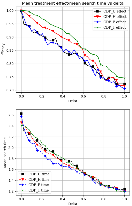
Figure S2 shows the trade-off between search time (number of trials) for different algorithms and 40 different values of with for samples, in the setting corresponding to Figure 2(b). In Figure S3, we give the corresponding comparison for using lower or upper bounds in the estimation of the stopping criterion , as described in Appendix A.3. Here, _U refers to the upper bound, _L to the lower bound and _E is “exact” estimator, i.e. the empirical estimator of the exact expression for the stopping criterion, . At first glance, the output of the different algorithms using different bounds appear very similar. However, as we see in Figure S4, the trade-off induced by a specific value of varies greatly depending on the estimation strategy. This is discussed also in Section 6, where we note that the policy learned by NDP is very sensitive to the setting of .

C.2 Antibiotic resistance dataset
Below, we give additional information on the antibiotic resistance dataset compiled from MIMIC-III.
To gather a cohort for which a consistent set of culture tests had all been performed for every patient, the set of organisms were restricted to a small subset. This selection was made based on overall prevalence in the data as well as the co-occurrence with common antibiotic culture tests. The selected organisms and antibiotics are listed below.
Selected (bacterial) microorganisms:
- •
Escherichia Coli (E. coli)
- •
Pseudomonas aeruginosa
- •
Klebsiella pneumoniae
- •
Proteus mirabilis
Selected antibiotics:
- •
Ceftazidime
- •
Piperacillin/Tazo
- •
Cefepime
- •
Tobramycin
- •
Gentamicin
- •
Meropenem
pending was also an “result” in MIMIC-III, there were few of these instances and they were removed. Covariates X: Ages are divided into the four groups , , , and . The two diseases are Infectious And Parasitic Diseases and Diseases Of The Skin And Subcutaneous Tissue as classified by ICD (WHO 1978). The data was split in training and test 70/30 from 1362 patients and patients with multiple organisms were not split between the sets. Patients who had taken any antibiotic other than our chosen ones were not included in the data. Figure S5 uses the same data as Figure 3(b) but is split by and variance is shown.
| # of treatments | # of patients |
| 1 | 860 |
| 2 | 340 |
| 3 | 137 |
| 4 | 22 |
| 5 | 3 |