University of Cape Town
Faculty of Science
Department of Mathematics and Applied Mathematics
Investigating Chaos by the Generalized Alignment Index (GALI) Method
Author:
Henok Tenaw Moges
Supervisor:
A/Prof Haris Skokos
March, 2020
![[Uncaptioned image]](2007.00941v1/UCT_logo.png)
Abstract
One of the fundamental tasks in the study of dynamical systems is the discrimination between regular and chaotic behavior. Over the years several methods of chaos detection have been developed. Some of them, such as the construction of the system’s Poincaré Surface of Section, are appropriate for low-dimensional systems. However, an enormous number of real-world problems are described by high-dimensional systems. Thus, modern numerical methods like the Smaller (SALI) and the Generalized (GALI) Alignment Index, which can also be used for lower-dimensional systems, are appropriate for investigating regular and chaotic motion in high-dimensional systems. In this work, we numerically investigate the behavior of the GALIs in the neighborhood of simple stable periodic orbits of the well-known Fermi-Pasta-Ulam-Tsingou lattice model. In particular, we study how the values of the GALIs depend on the width of the stability island and the system’s energy. We find that the asymptotic GALI values increase when the studied regular orbits move closer to the edge of the stability island for fixed energy, while these indices decrease as the system’s energy increases. We also investigate the dependence of the GALIs on the initial distribution of the coordinates of the deviation vectors used for their computation and the corresponding angles between these vectors. In this case, we show that the final constant values of the GALIs are independent of the choice of the initial deviation vectors needed for their computation.
Plagiarism declaration
I know the meaning of plagiarism and certify that this dissertation is my work, based on my study and I have acknowledged all the materials and resources used in the preparation.
![[Uncaptioned image]](2007.00941v1/Signature.png)
Henok Tenaw Moges
Acknowledgments
First and foremost, I would like to express my sincere gratitude to my supervisor, A/Prof Haris Skokos, for his continuous support and guidance. I am so grateful to have a supervisor who cares about my work. I would also like to thank A/Prof Thanos Manos for several useful discussions. I will forever be thankful to my colleagues in the ‘Nonlinear Dynamics and Chaos’ group”; Bob Senyange, Many Manda, Malcolm Hillebrand, and the former group member Chinenye Ani. Thank you, guys. I would like to pay my special regards to the Department of Mathematics and Applied Mathematics of the University of Cape Town (UCT) as well. This work was fully funded by the Woldia University and the Ministry of Science and Higher Education of Ethiopia and partially supported by the UCT International and Refugee Grant 2019. Finally, I would like to thank the High-Performance Computing facility of UCT and the Center for High-Performance Computing for providing the computational resources needed for this work.
List of abbreviations
- •
dof : degrees of freedom
- •
FPUT : Fermi-Pasta-Ulam-Tsingou
- •
GALI : Generalized Alignment Index
- •
IC : Initial Condition
- •
LE : Lyapunov Exponent
- •
mLE : maximum Lyapunov Exponent
- •
D : -Dimensional
- •
PSS : Poincaré Surface of Section
- •
SALI : Smaller Alignment Index Method
- •
SI : Symplectic Integrator
- •
SVD : Singular Value Decomposition
Introduction
Dynamical Systems theory attempts to understand, or at least describe, changes over time that occur in physical and artificial systems. It consists of a set of subaltern theories that can be applied to solve complex problems in numerous fields, such as weather predictability [1], stochastic processes [2] and evolutions of astronomical systems [3]. Because of the remarkable applicability of this theory, it has become one of the top topics in modern scientific research. In particular, Hamiltonian systems of many degrees of freedom (dof) have been broadly used for a general study and a better understanding of energy transport and equipartition phenomena (see for example [6, 4, 5, 7, 8] and references therein). Equipartition phenomena are associated with the dynamical nature of motion fostered in the respective phase space namely, the regular or chaotic evolution of the system’s orbits [6]. A chaotic dynamical system is one in which nearby initial conditions (ICs) lead to very different states as time evolves. This means that small variations in ICs can lead to large, and frequently unpredictable, variations in final states.
A fundamental aspect in studies of dynamical systems is the identification of chaotic behavior, both locally, i.e. in the neighborhood of individual orbits and globally, meaning for large samples of ICs. There are several ways to identify the chaotic behavior of a given nonlinear system. The rapid and efficient detection of the regular or chaotic nature of motion in many dof systems has been a very active research topic over the years. The most commonly used method to characterize chaos is the computation of the Lyapunov Exponents (LEs) [9, 10, 11, 12, 13]. In general, LEs are asymptotic measures characterizing the average rate of growth or shrink of small perturbations to the orbits of dynamical systems. The development of efficient algorithms for the calculation of LEs [11, 12] (see also [13] for a recent review on this topic) led to a gallery of chaos detection methods (see e.g. [14, 15, 16, 17]). The most commonly employed chaos indicators were recently reviewed in [17].
This study focuses on the Generalized Alignment Index (GALI) method [18], an efficient and fast chaos detection technique that can be used effectively for the description of the behavior of multidimensional systems. As its name would suggest, the GALI is a generalization of the Smaller Alignment Index (SALI) [19]. The main advantages of the GALI method are its ability to distinguish between regular and chaotic motion more quickly than other techniques and to determine the dimensionality of the torus on which the quasi-periodic motion occurs. In addition, it can predict slow diffusion in multidimensional Hamiltonian systems [20]. A concise overview of the theory and numerical applications of the SALI and the GALI methods can be found in [21].
Here we aim to understand the GALI’s prediction efficiency and performance when the IC of an orbit moves gradually from a regular to a chaotic motion region in Hamiltonian systems, by studying in detail the variation of the asymptotic values of the indices. This transition can take place either by changing the total energy of the system or by moving the regular orbit’s IC towards the edge of a stability island. In addition, we follow the time evolution of the deviation vectors, which are small perturbations of the IC and are needed for the computation of the GALIs, and examine if different initial distributions of the coordinates of these vectors affect the final GALI value. Our investigation was performed in phase space regions around some simple, stable, periodic orbits of the Fermi-Pasta-Ulam-Tsingou (FPUT) model [22, 23], which describes a chain of harmonic oscillators coupled through nonlinear interactions. The dynamics of this system has been studied extensively in the last decades (see e.g. [24, 25] and references therein) and this model is considered nowadays as a prototypical, multidimensional, nonlinear system.
Moreover, an investigation of the behavior of the GALIs for regular orbits of coupled area-preserving standard mappings [26] was carried out. More details on this mapping can be found in [27]. In some sense, our study completes some previous works on the GALI method [18, 20] where other aspects of the index have been investigated, for example, its behavior for periodic orbits [28].
The thesis is organized as follows:
- 1.
Chapter 1 provides a general overview of the general theory of Hamiltonian mechanics and chaotic dynamics. The Hamiltonian formulation of finite-dimensional systems is also presented.
- 2.
In Chapter 2, we present the symplectic integration methods used for our computations along with the introduction of several chaos detection techniques, namely the Poincaré Surface of Section (PSS), the LEs, as well as the SALI and the GALI methods. Particular emphasis is given to the properties and the numerical computation of the GALI method. In order to illustrate the behavior of the LEs, as well as the SALI and the GALI methods for regular and chaotic motion, simple Hamiltonian models and symplectic mappings are used: two-dimensional (2D) and four-dimensional (4D) mappings, as well as the 2D Hénon-Heiles system [29]. Moreover, the behavior of these indicators for dissipative dynamical systems is briefly discussed.
- 3.
In Chapter 3, aspects of the behavior of the GALI method in the case of multidimensional conservative Hamiltonian systems are investigated in detail. Most of the presented numerical simulations are performed using one of the most classical systems of statistical physics: the FPUT model [22]. The equations of motion and variational equations of this model are presented. The asymptotic behavior of the GALI for regular orbits in the neighborhood of two simple periodic orbits of the FPUT model is analyzed. An investigation of the dynamical changes induced by the increase of the coupling between the 2D mappings and their influence on the behavior of the GALI using a coupled standard mapping [27, 21] is also undertaken.
- 4.
In Chapter 4, we finally summarize and discuss the results and findings of our study.
Chapter 1 Hamiltonian mechanics
1.1 Overview of dynamical systems
The phase space of a dynamical system is the collection of all possible states of the system in question. Each state represents a complete snapshot of the system at some moment in time. The dynamical evolution of the system is governed by rules which transform one point in the phase space, representing the state of the system “now”, into another point representing the state of the system one time step “later”.
There are two different classes of dynamical systems:
- 1.
Discrete dynamical systems. They are described by recurrence relations iterated mappings or sets of difference equations
(1.1) where is a set of functions and is the state vector at the discrete time , .
- 2.
Continuous dynamical systems. They are described by differential equations
(1.2) where is a vector of state variables, , is a vector field, and is the time-derivative, which we can write as . We may regard (1.2) as describing the evolution in continuous time of a dynamical system with finite-dimensional state of dimension . In component form, we write , 11 1 Notice that, here we do not use notations such as to explicitly denote vectors. In addition, we also write vectors as row or column matrices. and the system (1.2) is given as
(1.3)
1.2 Chaos
Lets briefly discuss the definition of chaos. Chaos theory in mechanics and mathematics, studies the apparently random or unpredictable behavior in systems governed by deterministic laws. A more accurate term, deterministic chaos, suggests a paradox because it connects two notions that are familiar and commonly regarded as incompatible [30]. The first is that of randomness or unpredictability, for example in the trajectory of a molecule in a gas or the voting choice of a particular individual in a population. Usually, randomness is considered more apparent than real, arising from the ignorance of several causes in an experiment. In other words, it is commonly believed that the world is unpredictable because it is too complicated. The second notion is that of deterministic behaviors/laws, like for example the ones appearing in the motion of a pendulum or a planet, which have been used since the time of Isaac Newton, exemplifying the success of science in predicting the evolution of cases which are initially considered complex.
Devaney’s definition of chaos: we present here a formal definition of chaos following the presentation of [31]. Let be a metric space, where is a set which could consist of vectors in and is the distance or metric function. A function is called chaotic if and only if it satisfies the following three conditions:
- 1.
has sensitive dependence on ICs. This means that such that for any open set and for any point , there exists a point such that for some , where denotes successive application of . The positive real number is called a sensitivity constant and it only depends on the space and function .
- 2.
is topologically transitive. Thus, for any two open sets and there exists such that .
- 3.
The set of periodic points of is dense. A point is called periodic if for some .
This definition of chaos is widely used and accepted. To classify a dynamical system as chaotic the above three properties, i.e. the system being sensitive to ICs and topologically transitive, as well as having dense periodic orbits must be fulfilled. Sensitivity to ICs captures the idea that in chaotic systems minor errors or inaccuracies in the initial states can lead to large divergences in the system’s evolution. In other words, small changes in the IC of the system can lead to very different long-term trajectories. Usually, the first condition is mainly considered as the central idea of chaos in physical systems although the last two properties are also relevant from a mathematical point of view.
1.3 General theory of Hamiltonian systems
Newton’s second law gives rise to systems of second-order differential equations in and so to a system of first-order equations in , i.e. in an even-dimensional space. If the forces are derived from a potential function, the equations of motion of the mechanical system have many special properties, most of which follow from the fact that the equations of motion can be derived from a Hamiltonian formulation. The Hamiltonian formalism is the natural mathematical structure in which to develop the theory of conservative dynamical systems.
In a Hamiltonian system with dof, the dynamics is derived from a Hamiltonian function
| (1.4) |
where and are respectively the system’s canonical coordinates and momenta. An orbit in the -dimensional (D) phase space of this system is defined by the state vector
| (1.5) |
where , and .
1.3.1 Time independent Hamiltonian systems
In many cases, the Hamiltonian does not explicitly depend on time and the energy
| (1.6) |
is conserved along trajectories, i.e. it is a constant of motion [32]. Examples of such systems are the pendulum, the harmonic oscillator, dynamical billiards or the motion of a particle with mass in a potential described by the Hamiltonian
One might ask, when is the energy conserved? The answer to this question is given by the Noether‘s theorem [33]. This theorem applies to any action in classical mechanics weather it is described in the Lagrangian or Hamiltonian formulation. Focusing on Hamiltonian systems, let us consider a general action described by
| (1.7) |
and its Poisson bracket
| (1.8) |
where and are general functions of the generalized coordinates and , for . The system’s equations of motion are
The time derivative of a function of the canonical variables, which could explicitly depend on time , is expressed in terms of Poisson brackets as
| (1.9) | |||||
Let us assume that we are interested in a quantity which is conserved under the dynamics. Then Equation (1.9) indicates that
| (1.10) |
In many cases of practical interest, the quantity has no explicit time dependence and then Eq. (1.10) reduces to having the Poisson bracket of with the Hamiltonian equal to zero, i.e. . For example in the case of the free motion of a unit mass particle on the plane, which is described by the Hamiltonian , the angular momentum is a constant of motion as .
If the Hamiltonian function (1.4) of a system does not explicitly depend on time then it is an integral of motion, i.e. its value is conserved
because from Eq. (1.10) we see that . This behavior can be interpreted as follows: under stable conditions, performing an experiment today or tomorrow one expects to get the same results. In other words, for autonomous dynamical systems (i.e. systems which do not explicitly depend on time ) the system’s evolution is independent of the choice of the initial time value .
1.3.2 Equations of motion and variational equations
Consider a continuous autonomous Hamiltonian system (1.6) with dof described by variables , . The time evolution of an orbit of this system is governed by Hamilton equations of motion
| (1.11) |
where
with and being the identity and zero matrices, respectively, and
The time evolution of an initial deviation vector at time , , from a given orbit with ICs is defined by the so-called variational equations [13]:
| (1.12) |
where is the Hessian matrix with elements
| (1.13) |
with . Eq. (1.12) can be considered as the Hamilton equations of motion of the so-called tangent dynamics Hamiltonian of (1.6)
| (1.14) |
Let us now consider the D area-preserving 22 2 Any mapping is area-preserving if , , where is the D measure of . symplectic mapping (1.1) of discrete time. The evolution of deviation vector at time , related to a reference orbit , is the so-called the tangent map
| (1.15) |
where
| (1.16) |
is the system’s Jacobian matrix.
The evolution of the deviation vectors is needed for the computation of the chaos indicators. For a continuous Hamiltonian system, this evolution is done along the simultaneous integration of the equations of motion. In the case of symplectic mappings, the evolution of the deviation vectors is computed by simultaneously iterating the mapping (1.1) and the tangent map (1.15).
Chapter 2 Numerical techniques and models
2.1 Numerical integration: Symplectic Integrators
Symplectic integrators (SIs) are numerical schemes aiming to determine the solution of Hamilton equations of motion, preserving at the same time the Hamiltonian system’s underlying symplectic structure [34, 36, 35, 37, 38]. An advantage of SIs is that their application transforms the numerical integration of the Hamilton equations of motion into the application of a symplectic mapping. The use of SIs is facilitated by the presence of a separable Hamiltonian function, i.e. when the whole Hamiltonian system can be written as a sum of Hamiltonian terms, whose solution is known explicitly.
Let us present a general way of constructing explicit SIs for the separable Hamiltonian
| (2.1) |
where is the system’s kinetic energy and is the potential energy, following an approach based on Lie algebraic notion, Eq. (1.11) can be simply expressed as (see e.g. [35])
| (2.2) |
where is a differential operator defined by the Poisson bracket . The solution of this set of equations, for ICs = is formally given as
| (2.3) |
In the common case of Eq. (2.1) the Hamiltonian function can be split into two integrable parts as , with being the kinetic energy , which is a function of only the momenta , and being the potential energy depending only on the coordinates . A symplectic scheme for integrating (2.2) from time to , with being the integration step, consists of approximating the operator by an integrator of steps involving products of operators and , , which are exact integrations over times and of the integrable Hamiltonian functions and . and being carefully chosen constants in order to improve the accuracy of the integration scheme. Thus, a SI approximates the action of the operator of by a product of the form
| (2.4) |
where and are constants such that and is the so-called order of the integrator. Each operator and corresponds to a symplectic mapping, and consequently the product appearing on the right-hand side of Eq. (2.4) is also a symplectic mapping. Various approaches have been developed over the years in order to determine the values of the coefficients and resulting to schemes of different orders (see e.g. [39, 40, 34, 42, 41, 36, 37, 38] and references therein).
2.1.1 Second order symplectic integrators
A basic second order SI can be written in the form
| (2.5) |
like for example: the so-called leapfrog method having three steps (i.e. number of applications of the simple operator and ) with constants and . Thus
| (2.6) |
Let us now present some other 2nd order SIs like the 5 step SABA2 SI with composition constants and
| (2.7) |
and the SBAB2 scheme with constants and [42]
| (2.8) |
Another SI of this kind is the 9 step ABA82 scheme [36]
| (2.9) |
where
2.1.2 Fourth order symplectic integrators
A 4th order SI can be obtained by a symmetric repetition (product) of 2nd order SIs (2.5) in the form
| (2.10) |
where and are two real adequately determined constants. The construction can lead to the integrator developed by Forest and Ruth [39] involving 7 step
| (2.11) |
with composition constants
The second order schemes (2.7) and (2.8) can be used to derive the 9 step fourth order SI SABA4 and SBAB4 [42] with constants . Higher order coefficients for this family of SIs is found in [42].
2.1.3 Sixth order symplectic integrators
Once a 4th order SI is found, it is easy to obtain a 6th order scheme using the 4th order and implementing the same composition process, i.e.
| (2.12) |
An example of this construction is the SI developed in [34] which has 19 steps.
More generally, if a SI of order , , is already known, a SI of order can be obtained through the composition
| (2.13) |
with
2.2 Chaos detection methods
2.2.1 The Poincaré Surface of Section (PSS)
An efficient numerical technique for visualizing the behavior of a dynamical system is the so-called PSS (see for e.g. [29, 6]) which is named after Henri Poincaré. According to this method the dynamics in the phase space of a high-dimensional system is understood by observing the behavior induced by the flow on a particular section of the phase space. In particular, the dynamics is represented by the successive intersections of orbits with the PSS when this section is crossed in the same direction. In this way, a mapping is defined (see Fig. 2.1). The created Poincaré mapping is a discrete dynamical system which represents the continuous flow of the original dynamical system.

Let us discuss this in more detail by considering an D dynamical system defined by the set of ordinary differential equations
| (2.14) |
Let be an D PSS. This surface must be transverse to the flow, meaning that all trajectories starting on should cross it and should not evolve parallel to it. The Poincaré mapping is a mapping , which is obtained by following trajectories from one intersection after the other. Let us denote by the th intersection of an orbit with the PSS, , and define the Poincaré mapping as
| (2.15) |
If is a fixed point of the mapping, the trajectory starting at this point comes back after some iterations (equivalently after some time of the original dynamical system). Indicating that this is a periodic orbit of the original system (2.14). This fixed point corresponds to an -periodic orbit of the Poincaré mapping (2.15).
An efficient numerical approach to determine the Poincaré mapping of a dynamical system was proposed by Hénon [44]. Let us discuss this approach in more detail. Given an D autonomous dynamical system of the form of Eq. (2.14),
| (2.16) |
the PSS can be defined by a function of the form
| (2.17) |
Then () implicitly defines the Poincaré mapping of dimension . Usually we define the PSS by a function of the form where is a constant number. In order to find the crossing points of a trajectory with the PSS defined by , Hénon introduced in [44] a simple idea using a system of differential equation which is equivalent to the system () by using as the independent integration variable instead of time
| (2.18) |
2.2.2 Lyapunov Exponents
The LEs were introduced by Lyapunov [9] and they measure the exponential divergence of nearby orbits in phase space. LEs are quantities which measure the system’s sensitive dependence on ICs, i.e. the rate at which the information is lost as the system evolves in time.
The maximum Lyapunov Exponent (mLE), (see [13] and references therein), is the average rate of divergence (or convergence) of two neighboring trajectories in the phase space of a dynamical system and it is given by
| (2.19) |
where the operator maps the deviation vector from the tangent space at one point of the trajectory to the tangent space of the next point along the orbit. Practically the mLE can be computed as the limit for of the quantity
| (2.20) |
which is usually called finite-time mLE [13]. In (2.20) and are deviation vectors from a given orbit, at times and , respectively, and denotes any norm of a vector. Taking the limit as time goes to infinity, we have
| (2.21) |
We note that the direct application of Eq. (2.20) faces some computational problems [11] as in general, it results in an exponential increase of in the case of chaotic orbit. More specifically, with increasing this norm rapidly exceeds the possibilities of ordinary numerical computations. Luckily, this can be avoided by taking into account the linearity of the evolution operator and the composition law of these mappings [45]. So the quantity can be computed as
| (2.22) |
where , is a small time interval of the integration where time , . Then after time the deviation vector is renormalized in order to avoid overflow problems. The mLE, in the case of autonomous Hamiltonian systems, is positive for chaotic orbits whereas for regular orbits it goes to zero by following a power law [11].
2.2.3 The spectrum of LEs
The spectrum of LEs is another useful tool for estimating the stability and chaos of D dynamical systems. While the information from the mLE can be used to determine the regular or chaotic nature of orbits, the knowledge of part, or of the whole set of LEs, , provides additional information on the underlying dynamics and the statistical properties of the system as they can be used for example to measure the fractal dimension of strange attractors in dissipative systems [13]. Following [13] the ordering of the spectrum of LEs is given by
| (2.23) |
The sum of all LEs (i.e. ) measures the contraction rate of volumes in the phase space. In the so-called dissipative systems, , meaning that volumes visited by generic trajectories shrink exponentially. In autonomous Hamiltonian systems, , i.e. volumes are preserved. Similarly the sum of LEs for area-preserving symplectic mappings is zero
| (2.24) |
The LEs come in pairs of values having opposite signs
| (2.25) |
In addition, at least one pair of LEs is by default zero
| (2.26) |
Other vanishing exponents may signal the existence of additional constants of motion apart from the Hamiltonian itself.
For D Hamiltonian systems, the computation of the first LEs, with of an orbit is performed using the so-called standard method in [46]. This method involves the time evolution of initial linearly independent and orthonormal deviation vectors, with a new set of orthonormal vectors, obtained by the Gram-Schmidt orthonormalization process, replacing the evolved deviation vectors, along with the simultaneous integration of the equations of motions.
2.2.4 The Smaller Alignment Index (SALI) method
The idea behind the introduction of a simple, fast and efficient chaos indicator, such as the SALI [19, 21] was the need to overcome the slow limit convergence of (2.21). Instead of estimating the average rate of exponential growth, i.e. , SALI uses the possible alignment of any two normalized deviation vectors to identify the chaotic nature of orbits. In order to compute the SALI, we follow the evolution of the orbit and two deviation vectors, and . The SALI is computed at any unit time by [19]
| (2.27) |
where is either continuous or discrete time and and are unit vectors given by the relation
| (2.28) |
Note that SALI. SALI means the two deviation vectors, and align (i.e. both being either parallel or antiparallel) and SALI when the two vectors are perpendicular.
2.2.4.1 Properties of the SALI
The asymptotic behavior of the SALI for regular and chaotic motion is given as follows:
- 1.
In the case of regular motion SALI does not become zero [47]. The two deviation vectors, and , tend to fall on the tangent space of the torus, following a time evolution and having in general two different directions. Thus, in this case, SALI attains a constant positive value, i.e.
(2.29) - 2.
On other hand, for chaotic orbits, the deviation vectors align in the direction defined by the mLE and the SALI tends exponentially fast to zero at a rate which is related to the difference of the two largest LEs, and as discussed in [48], i.e.
(2.30)
Rather than evaluating SALI (2.27), in order to see if the two deviation vectors are aligned or not we can use the wedge product of these vectors [21]
| (2.31) |
which represents the area of the parallelogram formed by the two deviation vectors. Then indicates chaos and corresponds to regular motion. If we take more than two deviation vectors, say , , then the wedge product of the corresponding unit vectors evaluates the volume of the parallelepiped formed by these deviation vectors, which leads to the introduction of the GALI Method.
2.2.5 The Generalized Alignment Index (GALI) Method
Consider the D phase space of a conservative dynamical system represented by either a Hamiltonian flow of dof or a D symplectic mapping. In order to study whether an orbit is chaotic or not, we examine the asymptotic behavior of initially linearly independent deviations from this orbit, denoted by vectors , . Thus, we follow the orbit, using the Hamilton equations of motion or the mapping equations and simultaneously we solve the corresponding variational equations or the related tangent map to study the behavior of deviation vectors from this orbit.
The Generalized Alignment Index of order (GALIk) represents the volume of the generalized parallelogram defined by the evolved unit deviation vectors at any given time and it is determined as the norm of the wedge (or exterior) product of these vectors [18]
| (2.32) |
In the case that the number of deviation vectors exceeds the dimension of the system’s phase space, by definition the vectors will be linearly dependent and the corresponding volume (the value of GALIk, for ) will be zero.
2.2.5.1 Properties of the GALI
Let us consider dof Hamiltonian systems. For regular orbits, if we start with linearly independent initial deviation vectors, then the deviation vectors eventually fall on the D tangent space of the torus [18]. In this case, the asymptotic GALI value will be practically constant. Whereas, if we start with linearly independent initial deviation vectors, then the asymptotic GALI value will be zero since some deviation vectors will eventually become linearly dependent as again all of them will fall on the D tangent space of the torus. The general behavior of the GALIk for regular orbits lying on an D torus is given by [18]
| (2.33) |
We note that, the behavior of GALIk for regular orbits on lower-dimensional tori i.e. D torus with is given by [28].
| (2.34) |
On the other hand, for chaotic and unstable periodic orbits all deviation vectors align in the direction defined by the mLE and the value of GALIk decays exponentially fast to zero following a rate which depends on the values of several LEs [18, 28]
| (2.35) |
where are approximations of the largest LEs of the orbit. In particular when , GALI2 tends to zero exponentially fast as follows:
| (2.36) |
which is similar to the behavior of the SALI shown in (2.30). This is due to the fact that the SALI is equivalent to the GALI2 [18]. The behavior of the GALI2 for regular orbits in 2D mappings requires special attention. Since in this case the motion exists on a 1D torus, the two deviation vectors tend to fall on the tangent space of this torus, which is again 1D. Thus the two vectors will eventually become linearly dependent as in the case of chaotic orbits, but this happens with a different time rate given by [21]
| (2.37) |
where is the number of iterations.
An efficient way of computing the value of GALIk is through the Singular Value Decomposition (SVD) of the matrix
| (2.38) |
having as columns the coordinates of the unitary vectors [20]. Following [20] we see that the value of GALIk can be given by
| (2.39) |
where ‘’ denotes the determinant of a matrix . The matrix product in (2.39) is a symmetric positive definite matrix
| (2.40) |
where each element of th row and th column is the inner product of the unit deviation vectors and , so that
| (2.41) |
where is the angle between vectors and . Thus, the matrix of Eq. (2.40) can be written as
| (2.42) |
The value of the GALIk can be computed through the norm of the wedge product of the deviation vectors defined in (2.32) as
| (2.43) |
where the sum is performed over all possible combinations of indices out of (more details can be found in [18]). This means that in our computation we have to consider all the possible determinants of . From a practical point of view this technique is not numerically efficient for systems with many dof because of the large number of determinants in Eq. (2.43). Nevertheless, Eq. (2.43) is ideal for the theoretical treatment of the GALI’s asymptotic behavior for chaotic and regular orbits as has shown in [18].
According to the SVD method [49] the matrix can be written as the product of a column-orthogonal matrix , a diagonal matrix with non-negative real numbers , on its diagonal and the transpose of a orthogonal matrix :
| (2.44) |
Then the GALIk is computed using Eqs. (2.39) and (2.44) and by keeping in mind that , where is the unit matrix, since and are orthogonal. Thus,
| (2.45) | |||||
where , , are the so-called singular values of , obtained through the SVD procedure.
In our study, in order to compute the value of the GALIk we follow the time evolution of initially linearly independent random unit deviation vectors and implement the approach of Eq. (2.45). Furthermore, in order to statistically analyze the behavior of the GALIs we average the values of the indices over several different choices of the set of initial deviation vectors. The random choice of the initial vectors leads to different GALI values. Thus, in order to fairly and adequately compare the behavior of the indices for different initial sets of vectors we normalize the GALI’s evolution by keeping the ratio , i.e. we measure the change of the volume defined by the deviation vectors with respect to the initially defined volume. Another option is to start the evolution of the dynamics by considering a set of orthonormal vectors so that GALI. As we will see later on, both approaches lead to similar results, so in our study, we will follow the former procedure unless otherwise stated.
2.3 Illustrative applications to simple dynamical systems
Here, we consider some simple dynamical systems and use them to illustrate the behavior of the mLE, the SALI and the GALI for regular and chaotic orbits.
2.3.1 Conservative systems
2.3.1.1 Some Symplectic Mapping cases
Let us start our presentation by considering a simple area-preserving 2D symplectic mapping the so-called standard mapping [46]:
| (2.46) |
where is a real parameter and and denote the values of coordinates after one iteration of the motion. We note that all coordinates have (mod ), i.e. for .
Phase space portraits of the standard mapping for various values of the parameter are shown in Figure 2.2. More specifically, Fig. 2.2a shows that the phase space is practically filled with stability islands for a small value of the parameter . When we increase the value to (Fig. 2.2b), the stability islands become embedded within a chaotic sea represented by the scattered point zone. For , the chaotic sea dominates as we see in Fig. 2.2c.


The tangent map (1.15) of the 2D mapping (2.46) which is needed in order to compute chaos indicators is given by
| (2.47) |
We consider several orbits in the 2D mapping (2.46) for (Fig. 2.2b) for which it has both well defined chaotic and regular regions and we determine the nature of each orbit by using the following chaos indicators: the mLE and the SALI/GALI2. The obtained results are shown in Fig. 2.3. In order to to illustrate the behavior of the chaos indicators, we consider three different regular and chaotic orbits from Fig. 2.2b. The phase space portraits of the standard mapping (2.46) for these orbits is shown in Fig. 2.3a.
Fig. 2.3b shows that the mLE goes to zero for the regular orbits following an evolution which is proportional to the power law (which is indicated by the dashed straight line) whereas mLE eventually saturates to a constant value for chaotic orbits. Fig. 2.3c illustrates the time evolution of the SALI for the same regular and chaotic orbits. In the case of regular orbits, the evolution of the SALI is proportional to the theoretical prediction (2.37), while for chaotic orbits the SALI goes to zero exponentially fast following the exponential decay in (2.30). If we compare the time evolution of the mLE and SALI for chaotic orbits of Figs. 2.3b and 2.3c we can notice that SALI discriminates the chaotic orbits very fast.


Similar behaviors are also observed in the case of the 4D mapping [45, 50, 51]
| (2.48) |
Consisting of two coupled 2D standard mappings with parameters and , which are coupled through a term whose strength is defined by the parameter . In this case all coordinates , are given (mod ), i.e. .
Figures 2.4 to 2.6 show 2D projection of the 4D mapping for different values of by fixing the parameters and . In each case we iterated the mapping (2.48) by using five different ICs of the form , for , where , , , , . From the results of Fig. 2.4 we see that the considered orbits are mainly regular for except for the orbit with which shows a weak chaotic behavior. As the value of the coupling parameter increases to (Fig. 2.5) and (Fig. 2.6) more orbits become chaotic.


The tangent map of system (2.48) is given by
| (2.49) |
Let us consider the orbits of the 4D mapping (2.48) with ICs and as a representative of a regular (blue points in Fig. 2.6) and and for a chaotic orbit (red points in Fig. 2.6). In Fig. 2.7a we plot the four LEs for the regular and the chaotic orbit. For regular orbit, the LEs go to zero following an evolution which is proportional to the power law . For the chaotic orbit, the LEs come in pairs of opposite values, i.e. and . For this reason, we plot , , , . The four finite time LEs eventually saturate to a constant value for the chaotic orbit. In Fig. 2.7b we see that the time evolution of the SALI for the regular orbit leads to a constant value whereas the SALI goes to zero exponentially fast for the chaotic orbit.


Furthermore, in Fig. 2.8 we computed the evolution of the GALIs for these two orbits of Fig. 2.7. In Fig. 2.8a we plot the evolution of GALI2, GALI3 and GALI4 for the regular orbit. We see that GALI2 eventually saturates to a non-zero constant value while GALI3 and GALI4 go to zero following respectively the asymptotic power law decays and . In Fig. 2.8b we see the evolution of GALI2, GALI3 and GALI4 for the chaotic orbit. In this case, the GALIs go to zero following an exponential decay which is proportional to , and for which is the estimation of the orbit’s mLE (see Fig. 2.7).


2.3.1.2 The Hénon-Heiles system
The Hénon-Heiles system is a prototypical 2D Hamiltonian dynamical system initially used in [29] to investigate the motion of a star in a simplified galactic potential. The star is assumed to move on the galactic plane with coordinates and . The Hamiltonian function of this system is
| (2.50) |
where and are the conjugate momentum. The system’s equations of motion are
| (2.51) |
In Fig. 2.9 we present the PSS of the Hénon-Heiles system (2.50) with , defined by the condition and . There ordered orbits correspond to closed smooth curves, while the chaotic orbits are represented by scattered points.

In order to compute chaos indicators like the mLE, the SALI and the GALI we also need to integrate the system’s variational equations
| (2.52) |
In our simulations we simultaneously integrated Eqs. (2.51) and (2.52) using the SABA2 SI scheme with an appropriate integration time step which keep the relative energy error below .
We compute the mLEs and the SALIs for three different regular orbits which are taken from the islands of stability around periodic orbits of different periods 11 1 An orbit , in the system’s phase space, is called periodic if , for a non-zero constant number (Fig. 2.10a). Their ICs are , , and for the regular orbits and , , and for the chaotic ones. Fig. 2.10b shows that the mLEs go to zero for regular orbits following an evolution which is proportional to the power law , while they eventually attain constant positive values for chaotic orbits. In Fig. 2.10c we present the time evolution of the SALIs for the same regular and chaotic orbits. In the case of regular orbits, the SALIs obtain non-zero constant values. On the other hand, the SALIs go to zero exponentially fast for chaotic orbits. Similar to the discrete system of Section 2.3.1.1 (Figs. 2.3 and 2.7). The SALIs discriminate chaotic orbits very fast.


In Fig. 2.11 we also study the behavior of the GALIs for the regular orbit with IC and , and the chaotic orbit with IC and . The regular orbit lies on a 2D torus and therefore its GALI2 eventually saturates to a non-zero constant value, whereas the GALI3 and the GALI4 go to zero respectively following the asymptotic power law decays and (Fig. 2.11a). The GALIs for the chaotic orbit are shown in Fig. 2.11b. All of them go to zero exponentially fast following the exponential decays which are described in Eq. (2.35).


Overall all the methods we implemented can correctly capture the dynamical nature of the studied orbits. GALIk, with higher-order , is the fastest in discriminating between regular and chaotic motion whereas the mLE is the least efficient technique. For example, consider the evolution of the GALI4 and the mLE for the 4D mapping (2.48) and 2D Hamiltonian (2.51). The exponential decay of the GALI4 for the chaotic orbit with IC and (black curve in 2.8b) of (2.48) reaches the value around time , while the mLE (red curve in 2.7a) clearly indicates that the orbit is chaotic around time . Also, the exponential decay of the GALI4 for the chaotic orbit with IC and (black curve in 2.11b) of (2.51) reaches the value around time , while the mLE (purple curve in 2.10b) shows that the orbit is chaotic around time . Based on our results and discussion, we can conclude that the GALI method is the most effective among the methods we have considered. Even though the convergence of the LEs is theoretically guaranteed, its rate of convergence can become too slow, while the PSS is impractical for systems with many dof.
2.3.2 Dissipative systems
A dynamical system is called non-conservative if its phase space volume changes over time. The determinant of the system’s Jacobian matrix is an important tool to explore the properties of the dynamic, in particular to describe the change in volume. If this determinant is smaller than one, then the volume of phase space decreases over time [52].
For dissipative systems, in the limit of the dynamics converges to a set of values for various ICs, the so-called attractor. A dynamical system can have several different attractors. We should note that the concept of an attractor is only relevant when discussing the asymptotic behavior of orbits.
In this section, we compute various chaos indicator of two dissipative systems. The aim is to briefly investigate the behavior of the GALIs for these systems. Our results suggest that further work is certainly required. However, this study provides a good starting point for further investigations.
2.3.2.1 The Hénon Mapping
First we consider a mapping which was introduced by Hénon [53] based on concepts of stretching and folding of areas in the phase space. The Hénon mapping takes a point in the plane and maps it to a new point according to the rule
| (2.53) |
According to [53], the dynamics converges to a strange attractor for parameter values and . This attractor is seen in Fig. 2.12

The rate of expansion of an area in the map’s phase space is given by the determinant of the Jacobian matrix of the mapping (2.53)
| (2.54) |
Thus for the mapping is area preserving but when , as we have done for the case , the mapping is dissipative and phase space areas contract.
There is an equally simple (as the Hénon mapping (2.53)) 2D quadratic mapping admitting several attractors [54]. This mapping, has two parameters, and , and it is given by
| (2.55) |
Note that this mapping is conservative for values of the parameter . The associated tangent map of the 2D quadratic mapping (2.55) is given by
| (2.56) |
We compute the LEs as well as the SALI of the mapping (2.55) of a representative regular and a chaotic orbit. For the regular orbit we use the parameters and the IC , . In Fig. 2.13a we plot the evolution of the two LEs of this orbit. We see that the LEs eventually attain negative values for this regular orbit, i.e. and . Fig. 2.13b displays the time evolution of the SALI for this orbit. We see that, the SALI remains practically constant.


In Fig. 2.14 we use the parameters for the mapping (2.55) and compute the chaos indicators for the chaotic orbit with IC . Fig. 2.14a shows the evolution of two LEs for this orbit. We see that the two finite time LEs eventually saturate to positive constant values and . In Fig. 2.14b we plot the evolution of the SALI for the same orbit and we can see that it goes to zero exponentially fast.


2.3.2.2 The case of a 4D mapping
Similar behaviors are observed for a more complicated mapping model given by [55]
| (2.57) |
where , and , is the dissipation parameter, are randomly generated noise variables, within the interval , and , , . The corresponding tangent map is given by
| (2.58) |
where . Mapping (2.57) is conservative when .
We also studied the time evolution of the mLE and the GALIk, of mapping (2.57) for a regular and chaotic orbit. From Fig. 2.15a we see that the mLE reaches a negative constant value for the regular orbit () with IC when the mapping parameters are set to , , , , . Whereas it becomes positive value for the chaotic orbit with IC when the mapping parameters are set to , , , , () (Fig. 2.16a). In Fig. 2.15b we can see that the GALIs remain practically constant for the regular orbit while they go to zero exponentially fast for the chaotic orbit (Fig. 2.16b).


Chapter 3 Behavior of the GALI for regular motion in multidimensional Hamiltonian systems
3.1 The Fermi-Pasta-Ulam-Tsingou (FPUT) model
The FPUT model [22, 23] describes a multidimensional lattice system and it is related to the famous paradox of the appearance of a recurrent behavior in a nonlinear system. It is traditionally called the FPUT model and represents a one-dimensional chain of identical particles with nearest-neighbor interactions (see Fig. 3.1).

The FPUT Hamiltonian is
| (3.1) |
where is the displacement of the th particle from its equilibrium position and is the corresponding conjugate momentum. In our study we impose fixed boundary condition to system (3.1), i.e. . We also chose to work with the FPUT system (i.e. in (3.1))
| (3.2) |
because it does not allow particles to escape.
In order to use a SI scheme for the integration of the system’s equations of motion and variational equations (using the so-called tangent map method [35, 56, 57]) we split the Hamiltonian in two integrable parts in which is a function of the momenta and is a function of the coordinates :
| (3.3) |
Then the corresponding equations of motion for the Hamiltonian functions and , for , are
| (3.4) |
and
| (3.5) |
These two sets of differential equations can be easily integrated. The operators and which propagate the set of ICs and at time to , , and time ( being the integration time step), for , are
| (3.6) |
and
| (3.7) |
Computational considerations
Here we discuss some practical aspects of our numerical simulation. In order to compute the time evolution of GALIk of a dof Hamiltonian system, we need initially linearly independent deviation vectors. In most considered cases the coordinates of these vectors are numbers taken from a uniform random distribution in the interval . To statistically analyze the behavior of the GALIs their values are averaged over several different choices of sets of initial deviation vectors. In particular, we use sets of initial vectors. The random choice of the initial vectors leads to different GALI values, i.e. the value of the GALIk at the beginning of the evolution. Thus, to fairly and adequately compare the behavior of the indices for different initial sets of vectors we normalize the GALIs’ evolution by registering the ratio GALI/GALI, i.e. we measure the change of the volume defined by the deviation vectors with respect to the initially defined volume. Another option is to start the evolution of the dynamics by considering a set of orthonormal vectors so that GALI. As we will see later on, both approaches lead to similar results, so in our study we will follow the first procedure, unless otherwise specifically stated.
In our investigation, we implement an efficient fourth-order symplectic integration scheme the so-called ABA864 method, to integrate the equations of motion and the variational equations of the FPUT system (3.2). In our numerical simulations, we typically integrate the FPUT system (3.2) up to a final time of time units. By adequately adjusting the used integration time step we always keep the absolute relative energy error 11 1 The relative energy error, , is defined as , where is the computed Hamiltonian value at the current time unit and is the initial Hamiltonian value. below .
The scope of our work is to quantitatively analyze the chaotic and regular behavior of orbits of the multidimensional FPUT model (3.2). In Chapter 2, we described in detail the behavior of the mLE, and the spectrum of LEs, as well as of the SALI and the GALI for 2D and 4D systems. These behaviors should hold for multidimensional systems. In order to illustrate the behavior of these indices let us take the -FPUT model (3.2) with dof and consider some typical regular and chaotic orbits. More specifically we consider the regular orbit with total energy and ICs , , , , , and and the chaotic orbit with total energy and ICs , , , , , , and .
The evolution of the mLE for these orbits is shown in Fig. 3.2a while their SALI is depicted in Fig. 3.2b. In Fig. 3.2a, we see that for the regular orbit (blue curve) the mLE goes to zero with a decrease proportional to the function whereas the remains practically constant for the chaotic orbit (red curve), which is exactly what we expect from a chaotic trajectory. In Fig. 3.2b we see that SALI goes to zero exponentially fast following the law of (2.30), i.e. SALI for and , which are good estimations of the first and the second largest LEs. On the other hand, it remains practically constant and different from zero for the regular orbit (blue curve).


In Fig. 3.3 we plot the whole spectrum of LEs consisting in total of 16 LEs, for orbits and . In the case of the regular orbit (Fig. 3.3a) all 16 LEs approach zero following an evolution proportional to , while in the case of the chaotic orbit (Fig. 3.3b) the set of LEs consist of pairs of values having opposite signs. Positive LEs are plotted in green while negative values in red. Moreover, two of the exponents, and (yellow curves in Fig. 3.3b), eventually become zero. We will use the values of these 16 exponents later on when we will discuss the results of Fig. 3.5.


Let us now study the behavior of the GALIs for these two orbits. The regular orbit lies on an torus and therefore GALI2 up to GALI8 eventually oscillate around a non-zero constant value which decreases with increasing order (Fig. 3.4a), while the GALIs with order greater than the dimension of the torus go to zero following the asymptotic power law decays in accordance with Eq. (2.33) (Fig. 3.4b). On the other hand, the GALIs of the chaotic orbit follow exponential decays in accordance with Eq. (2.35) (Fig. 3.5).


3.2 The behavior of the GALIs for regular orbits
For Hamiltonian flows and symplectic maps, a random small perturbation of a stable periodic orbit in general leads to regular motion. Hence, finding a stable periodic orbit of the FPUT system (3.2) and performing small perturbations to it will allow us to study the behavior of GALI for several regular orbits.
The eigenvalues and eigenvectors of the so-called monodromy matrix dictate the stability of the periodic orbit. is the fundamental solution matrix of the variational equations of the periodic orbit evaluated at a time equal to one period of the orbit (see e.g. [58]). This matrix is symplectic, and its columns are linearly independent solutions of the equations that govern the evolution of deviation vectors from the periodic orbit, i.e. the variational equations. Since the Hamiltonian system (3.2) is conservative, the mapping defined by the monodromy matrix is volume-preserving, i.e. the determinant of is one. In addition, the product of the matrix eigenvalues, which is equal to the determinant, is also one.
If all the eigenvalues of are on the unit circle in the complex plane, then the corresponding periodic orbit is stable otherwise it is unstable. The instability can be of different types (more discussion about this can be found in [58] and references therein) but here we are only interested in the stability of periodic orbits. So we do not pay much attention to the types of instability periodic orbits have when they become unstable.
In an D autonomous Hamiltonian system, it turns out that two eigenvalues are always equal to [58]. In practice, the remaining eigenvalues define the stability of the periodic orbit. In addition, we expect the eigenvalues of computed at any point of the stable orbit to remain the same since the stability of the orbit does not change along the orbit. Thus, we can reduce our investigation to a D subspace of the whole phase space using the PSS technique (see e.g. [6]), where the corresponding monodromy matrix has eigenvalues, none of which is by default .
In our analysis, we investigate the behavior of the GALIs for regular orbits in the neighborhood of two simple periodic orbits (SPOs) of the FPUT system (3.2), which we refer to as SPO1 and SPO2. In the remaining part of our study, we set . The existence and dynamics of these SPOs for the FPUT system were discussed in [59, 60].
3.2.1 Regular motion in the neighborhood of SPO1
The first SPO we study is called SPO1 in [60] and it is obtained by considering the FPUT lattice (3.2) with being an odd integer so that all particles at even-numbered positions are kept stationary at all times, while the odd-numbered particles are always displaced symmetrically to each other. For example, when the 2nd, 4th and 6th particles are fixed, i.e. and the odd numbered particles, i.e. 1st, 3rd, 5th and 7th are equally displaced but in opposite directions, i.e. (see Fig. 3.6).

In general, the SPO1 for dof is given by
| (3.8) |
for . Using condition (3.8) in the system’s equations of motion we end up with a second order nonlinear differential equation for variable which describes the oscillations of all moving particles of the SPO1. In particular, for we have
| (3.9) |
while , for all times.
In Fig. 3.7 we see the arrangement of the eigenvalues of the monodromy matrix of the SPO1 orbit of Hamiltonian (3.2) with when (Fig. 3.7a) and (Fig. 3.7b). In the first case the SPO1 is stable as all eigenvalues are on the unit circle, while in the latter the orbit is unstable as two eigenvalues are off the unit circle.

The stability analysis of the SPO1 [59, 60] showed that for small values of (3.2) the orbit is stable, but it becomes unstable when the energy increases beyond a certain threshold . For instance in Fig. 3.7 the transition from stability to instability occurs at for particles. In [59, 60] the authors computed the energy density threshold for different number of particles , and they found that decreases as the value of increases following an asymptotic law . Fig. 3.8 illustrates the destabilization energy threshold for SPO1 with respect to increasing .

The main objective of our analysis is to study the behavior of GALIs for regular orbits that are located in the neighborhood of the stable periodic orbits. In order to find these regular orbits we initially start with the stable SPO1 having ICs , , and energy density . Then we perturb this orbit to obtain a nearby orbit with ICs , while keeping the total energy fixed. Practically, in order to find the perturbed orbit, we add a small random number to the positions of the stationary particles of the stable SPOs, i.e. we have , where s are small real random numbers. Then we change the position of one of the initially moving particles to keep the same energy value .
The phase space distance between these two orbits, , and , is given by
| (3.10) |
As we have already shown in Sec. 2.2, in multidimensional Hamiltonian systems, the value of the GALIk with remains practically constant for regular orbits lying on an D torus and these constant values decrease as the order of the index grows [20]. In order to improve our statistical analysis we evaluate the average value of over a set of different random initial deviation vectors and denote this quantity as . We stop our integration when the values of the GALIs more or less saturate showing some small fluctuations. Then we estimate the asymptotic GALIk value, denoted by , by finding the mean value of over the last recorded values and the related error is estimated through the standard deviation of the averaging process.
Fig. 3.9 shows the time evolution of for a regular orbit with distance from the stable SPO1 and . The gray area around these curves represents one standard deviation. We observe that GALIs of higher orders converge to lower values and need more time to settle to these values. In Fig. 3.9b we see more clearly how these final asymptotic values, , decrease with increasing .

Similar results are obtained for a regular orbit in the neighborhood of SPO1 for (Fig. 3.10). Again we observe that the almost constant final values of the GALIs drastically decrease as the order of the index increases from GALI2 to GALI21. Also, GALI21 starts saturating at around but GALI2 becomes constant around .

Now we focus our attention on the behavior of GALIs when the regular orbits depart from a stable periodic orbit moving towards the edges of the stability island, for a constant value of . We do that by perturbing the ICs of the stable periodic orbit by a small number, i.e. by increasing (3.10). Fig. 3.11 shows the outcome of this process. There we see how the behavior of GALIs change with increasing distance from the stable SPO1, when we only consider one set of initial deviation vectors. In particular, we see the evolution of three different GALIs, namely GALI2 (Fig. 3.11a), GALI4 (Fig. 3.11b), and GALI11 (Fig. 3.11c) for several orbits in the neighborhood of the stable SPO1 with and , , , , and . All values of GALIs for the smaller distance go to zero asymptotically following the power law of Eq. (2.33), i.e. GALI2 with [Fig. 3.11a], GALI4 with [Fig. 3.11b], and GALI11 with [Fig. 3.11c]. The behavior of the GALIs for the perturbed orbit with the smallest distance from the SPO1, , is still similar to what we expect for a stable periodic orbit. When we increase the asymptotic behavior of the GALIs start deviating from the above mentioned power decay law, and eventually GALIk becomes constant for , . Finally, for very large values the perturbed orbits will be outside the stability island. This happens for which leads to chaotic motions. In this case, GALIs go to zero exponentially fast. Note that the values of the GALIs for the regular orbit grow with increasing distance from the stable SPO1. In Fig. 3.12a we see the values of with respect to increasing when is kept constant to , for regular orbits around the SPO1 orbit. We chose an appropriate value for in order to avoid a transition to chaotic motion.

There is another way to move from stability to instability, that is by increasing the energy densities . We have seen in Fig. 3.8 that as long as we are below the destabilization energy of SPO1, the periodic orbit is stable. For instance, in the case of the SPO1 is stable below . In Fig. 3.12b we present the values of as a function of the GALI’s order for regular orbits in the neighborhood of the stable SPO1 for increasing energy densities . In particular, we consider regular orbits with for , for and with for and . Therefore, the values decrease as we increase the energy density for regular orbits around the stable SPO.

We have investigated the behavior of the GALIk for regular orbits in two ways. We showed that the asymptotic GALIk values change when we increase the distance of the studied orbit from the stable SPO1 for constant energy (Fig. 3.12a). We also saw that, the asymptotic value of GALIk decreases with increasing energy densities inside the stability island [Fig. 3.12b].
For example, for the stable SPO1 with and regular motion occurs up to . So, the motion of the perturbed orbits above this value is chaotic. Fig. 3.13 shows an approximation of the size of the stability island around the SPO1 orbit with different energy densities by finding the largest distance, denoted by , in which regular motion is observed for .

Similar results have been obtained in Fig. 3.14 for . In Fig. 3.14a we see the asymptotic, values for regular orbits in the vicinity of the stable SPO1 of the FPUT system (3.2) for with respect to increasing distances , , and , while in Fig. 3.12b we see how changes for and , and , and , and and .

3.2.2 Regular motion in the neighborhood of SPO2
So far our analysis was based on results obtained in the neighborhood of one SPO type, i.e. SPO1. We will now show that these findings are quite general as they remain similar for another SPO. In particular, to illustrate that a similar analysis is performed for regular orbits in the neighborhood of what was called SPO2 in [60].
The SPO2 of the FPUT system (3.2) with , , particles, corresponds to an arrangement where every third particle remains always stationary and the two particles in between move in opposite directions, i.e.
| (3.11) |
For example, for , particles located in the 3rd and 6th position do not move, , while the remaining consecutive particles are moving symmetrically and in opposite directions, i.e. (Fig. 3.15).

As in the case of the SPO1, we can obtain a single differential equation for the time evolution of the SPO2 when substituting (3.2.2) in the equations of motion of the FPUT system (3.2). In particular we get
| (3.12) |
for the moving particles, while for the stationary particles with .
In Fig. 3.16 we present the arrangement of the eigenvalues , , of the monodromy matrix of the SPO2 of Hamiltonian (3.2) with . In Fig. 3.16a all eigenvalues are on the unit circle, which means that the SPO2 with and is stable. We note that the monodromy matrix is evaluated on the PSS , . In Fig. 3.16b, there are four eigenvalues outside the unit circle, thus the SPO2, with and is unstable. In this case, the monodromy matrix is evaluated on the PSS , . The critical energy density for which the SPO2 encounters its first transition from stability to instability is much smaller that the one seen for SPO1. In particular, it is .

Similarly to Fig. 3.8 for the SPO1, the stability analysis of the SPO2 [59] determined the relation between the energy density threshold and the dimension of the system (Fig. 3.17). The first destabilization energy density of SPO2 follows a slower asymptotic decrease compared to SPO1, i.e. [59].
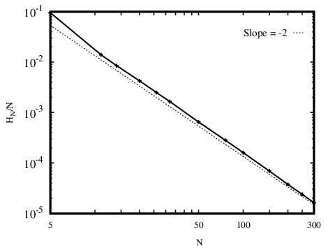
The estimation of the size of the stability island around the stable SPO2 with shows a similar behavior to what we observed for the same in the case of the SPO1 (Fig. 3.13). In Fig. 3.18 we report the maximum value of (i.e. ) for which regular motion occurs as a function of the energy density for the stable SPO2 of (3.2). Note that the energy axis is smaller than the one of Fig. 3.13 since the critical energy density for which the SPO2 becomes unstable for the first time is .

Similarly to Fig. 3.12 in Fig. 3.19a we see the dependence of on the order for increasing and constant , whereas in Fig. 3.19b we have similar results but for increasing values for regular orbits close to the stable SPO2 with .

In Fig. 3.20 we see the values for regular orbits around the stable SPO2 for . Note that the destabilization threshold of the SPO2 for is much smaller than in the case with .

The results of Figs. 3.19 and 3.20 clearly shows that the behavior of the asymptotic GALI values for regular orbits in the neighborhood of the stable SPO1 we have observed in Sec. 3.2.1, remains valid for the stable SPO2. The values increase when the regular orbit approaches the edge of the stability island (Figs. 3.19a and 3.20a) while it decreases when this orbit moves towards the destabilization energy ( Figs. 3.19b and 3.20b).
3.3 Statistical analysis of deviation vectors
Let us now turn our attention to the properties of the deviation vectors needed for the computation of the GALIs. Regular motions take place on a torus and the time evolution of all the initially linearly independent deviation vectors brings them on the tangent space of this torus, having in general different directions. On the other hand, in the case of chaotic orbits, the deviation vectors gradually align to the direction defined by the mLE following the exponential law given in Eq. (2.35).
We start our study by noting that the values of the GALIs are practically independent of the choice of the initial deviation vectors. To illustrate this property, we consider different sets of initial deviation vectors whose coordinates are drawn from three different types of probability distributions and compute the corresponding GALIs. In particular, we consider a uniform distribution in the interval (green curves in Fig. 3.21), a normal distribution (blue curves in Fig. 3.21) with mean 0 and standard deviation 1 in the interval , and an exponential distribution with mean 1 (red curves in Fig. 3.21). Fig. 3.21a displays the time evolution of for a regular orbit in the neighborhood of the stable SPO1 of Hamiltonian (3.2) for and . The average is done over sets of normalized unit (denoted by [u]) initial deviation vectors. Fig. 3.21b shows a similar computation but over sets of orthonormalized (denoted by [o]) deviation vectors, i.e. GALI. In Fig. 3.21c we compare asymptotic values, , obtained from the results of Figs. 3.21a and 3.21b. The curves are more or less the same. This indicates that the choice of the initial deviation vectors does not affect the values of the GALIs. The three curves corresponding to the different initial distribution of the vectors’ coordinates practically overlap both in Fig. 3.21a and 3.21b which is a clear indication that the time evolution of the GALIk is similar, irrespective of the used distribution.

Furthermore, we analyze the distribution of the coordinates of the vectors and the corresponding angles between these vectors (seen in Eq. (2.42)). In particular, we consider the two cases and . In Fig. 3.22a we show vector coordinates distributions obtained from the evolution of GALIk for a regular orbit of Hamiltonian (3.2) with which is close to the stable SPO1, with and . When we follow the time evolution of GALIk, using unit or orthonormal initial deviation vectors, the coordinates of the deviation vectors and the corresponding angles on the torus have the same distribution. We note that for GALIk with high order we obtain better statistics as we have in our disposal a large number of vectors and corresponding angles. Thus, considering, for example, GALIk with the largest possible order, i.e. GALI11, we obtain a fine picture of the distributions. More specifically, in order to follow the evolution of GALI11 we use initial deviation vectors with coordinates and angles. In Fig. 3.22a we plot the probability density distributions of the coordinates of the unit deviation vectors needed for the evaluation of GALI11 for a regular orbit close to the SPO1 of the Hamiltonian (3.2) with . The distributions are generated from the coordinates of sets of deviation vectors over snapshots when the GALI11 has reached its asymptotic value. A similar behavior is observed when increasing the number of particles. The time evolution of GALI21 for regular orbits of (3.2) with close to the stable SPO1 , using initial unit [u] and orthonormal [o] deviation vectors led to the creation of Fig. 3.22b where we plot the distributions obtained from the coordinates of sets of vectors as in Fig. 3.22a. The two curves, in both Figs. 3.22a and 3.22b practically overlap.

We further investigated how the distribution of the angles between each deviation vectors behaves and a behavior similar to that seen in Fig. 3.22 is obtained. Fig. 3.23a [Fig. 3.23b] displays the probability density distributions of the angles corresponding to the deviations in Fig. 3.22a [Fig. 3.22b]. The curves are almost the same, with distributions of the angles corresponding to vectors whose coordinates are drawn from the initial unit [u] and orthonormal [o].

Based on the results from Fig. 3.21 and Fig. 3.22 we can argue that the distribution of the coordinates of the initial deviation vectors does not affect the asymptotic behavior of the GALI. Therefore, we can, for example, use initial unit deviation vectors whose coordinates are drawn from a uniform distribution for our analysis.
So far we have investigated the behavior of the distribution of the coordinates of deviation vectors when the vectors have fallen on the tangent space of the torus, but it is interesting to also investigate the dynamics of the deviation vectors for the whole evolution of the regular orbit. In order to do so, we follow the evolution of GALI11 (Fig. 3.24a) for the regular orbit close to the stable SPO1 of (3.2) for , with and , and analyze in Figs. 3.24b and 3.24c the distributions of the coordinates of the deviation vectors by dividing the time evolution into five evenly spaced intervals, I1: (blue curves), I2: (green curves), I3: (red curves), I4: (black curves) and I5: (yellow curves). Fig. 3.24b shows the distribution of the coordinates of the deviation vectors for the five intervals. In Fig. 3.24c we see a similar distribution as in Fig. 3.24b but with different random sets of initial deviation vectors. In both cases, we can say that the time evolution of the GALIs does not depend on the sets of initial deviation vectors. Moreover, as the GALIs approach their constant asymptotic value (interval I5) the distribution of the coordinates of the deviation vectors has a sharply peaked shape with a high concentration in the middle.

Finally we evaluated the asymptotic coordinate distributions of the deviation vectors used to compute the GALIs for regular orbits in the neighborhood of the stable SPO1 Fig. 3.25a and Fig. 3.26a and SPO2 Fig. 3.25b and Fig. 3.26b orbits. In our computations we use 10 sets of 11 initially linearly independent unit deviation vector. In Fig. 3.25 we see the dependence of the final coordinate distribution of these vectors when the distance from the SPO is increased (for fixed values) for the stable SPO1 (Fig. 3.25a) and SPO2 (Fig. 3.25b) orbits. In Fig. 3.26 we see similar results as in Fig. 3.25 but when the orbits’ energy density increases for cases close to the stable SPO1 (Fig. 3.26a) and SPO2 (Fig. 3.26b) periodic orbits. In all considered cases for small values of and , the distributions have a peaked shape with a concentration in their middle. As the regular orbits get closer to the boundary of the stability island (increase D in Fig. 3.25 and increase E in Fig. 3.26) the distributions become more sharply peaked with a very high concentration in their centers.


3.4 A multidimensional area-preserving mapping
So far we have discussed the behavior of the GALIs for the FPUT Hamiltonian model (3.2) which has a continuous time . In particular, we have studied the asymptotic behavior of GALIs for regular orbits in the neighborhood of the stable SPOs when their distance from them increases. Here, we will implement the same methodology for regular orbits of a multidimensional area-preserving mapping in order to investigate the generality of our findings.
As we already discussed in Sec. 2.3, the standard mapping describes a universal, generic of area-preserving mapping with divided phase space in which the integrable islands of stability are surrounded by chaotic regions. A D system of coupled mappings is:
| (3.13) |
where indicates the new values of variables after one mapping iteration and is a dimensionless parameter that influences the degree of chaos, while is the coupling parameter between neighboring mappings where . All values have (mod ), i.e. , and also periodic boundary conditions are imposed: and .
For this coupled standard mapping model, the behavior of the GALIs for a given IC depends on the parameters , as strongly influences the regular or chaotic nature of the mapping’s orbits. Here, the objective is to show that what we have observed so far for the behavior of the GALIs in the case of the FPUT model (Sec. 3.2) and in particular the results of Figs. 3.9 and 3.11, hold also for the discrete system (3.13). In other words, we investigate the behavior of the GALIs when the transition of periodic orbits from regular to chaotic motion happens for the mapping (3.13) using the same analysis. In order to do this, we start from the center of the big island [27], for a small value of and coupling and we locate a stable periodic orbit. The location of this island is shown in Fig. 3.27 for the simple case of the 2D mapping (2.46)

As we have seen in Fig. 3.11 when the stable orbit is very close to the SPO, the GALIs tend to zero following the power law (2.34) (curve in Fig. 3.11). Then as the orbit’s IC is moved further and further away from the SPO the GALIs asymptotically tend to a positive value (curves to in Fig. 3.11) while when the orbit’s IC is outside the stability island the motion becomes chaotic and the GALIs will go to zero exponentially fast as it happens for the curve in Fig. 3.11. All these behaviors can also be observed for the mapping, Fig. 3.28 clearly illustrate these results. There we see the behavior of the GALIs for increasing distances from the center of the island of stability. In particular, the evolution of the GALI2 for different orbits starting in the neighborhood of the stable periodic orbit of (3.13) with parameters and , and distances , , , , and are shown in Fig. 3.28. We note that GALI2 for the periodic orbit () goes to zero asymptotically following the power law (2.33). Then, as the value of is increased the GALI2 gradually starts to saturate to a constant value ( to ). Finally, the perturbed orbit becomes unstable and the GALI2 goes to zero exponentially fast ().

In Fig. 3.29 we follow the evolution of the GALIk in a similar way to Figs. 3.9 and 3.10. From the results of Fig. 3.29a we see that the GALIk with higher order needs more time to become constant. For example, GALI20 asymptotically saturates around while GALI2 saturates faster around time units. From Fig. 3.29b we see that the final asymptotic value drastically decrease as the order of the index increases.

Chapter 4 Summary and discussion
In this work, we performed several numerical investigations of multidimensional dynamical systems by implementing several chaos detection techniques. In the first chapters of the thesis, we gave a brief overview of the basic notions of Hamiltonian dynamics along with a presentation of some basic numerical techniques for investigating chaos. The creation of the Poincaré surface of section is an important tool to understand the behavior of dynamical systems by representing trajectories of the full D phase space by an object in a D spaces, which is more suited for lower-dimensional dynamical systems. On the other hand, chaos indicators like LEs, SALI and GALI, can also be used for the same purpose, having the advantage of efficiently discriminating between regular and chaotic motion in high-dimensional systems. Initially, we discussed the LEs which measure the average rate of growth or shrinking of small perturbations to the orbits of a dynamical system. The mLE is a powerful tool to determine the chaotic and regular nature of an orbit, while the whole spectrum of LEs provides additional information on the dynamics of the system. Then we consider the SALI which is related to the area defined by two deviation vectors. It is an efficient and simple method to determine the ordered or chaotic behavior of orbits in dynamical systems. Generalizing the idea of the SALI leads to a computationally more efficient technique called the GALI method. The GALI of order (GALIk) represents the volume of a parallelepiped formed by initially linearly independent deviation vectors of unit length.
For the computation of these chaos indicators, a symplectic integration scheme was used to follow the time evolution of the equations of motion and variational equations of the Hamiltonian. In our presentation, we applied these indicators on the 2D Hénon-Heiles Hamiltonian, 2D and 4D symplectic mappings as well as on simple dissipative systems.
The main results of our work was presented in Chapter 3, where we thoroughly investigated the behavior of the GALI chaos indicator for regular motions in multidimensional Hamiltonian systems. In the case of stable periodic orbits, GALIk goes to zero following the power law described in [28], while it tends to zero exponentially fast following a rate that depends on the values of different LEs for unstable orbits. In our study, more attention was given to regular motions that lie on D tori, i.e. GALIk, asymptotically attain a non zero constant value. To analyze these asymptotic values of GALIs we considered several regular orbits in the vicinity of two basic simple periodic orbits of the FPUT model (3.2), namely, SPO1 and SPO2 orbits [60], for various numbers of the system’s degrees of freedom.
The main results of our study are the following: the asymptotic GALI values, , for regular orbits on D tori of multidimensional Hamiltonian models depend on:
- •
- •
- •
In addition, we computed the evolution of GALIs using initially linearly independent deviation vectors generated from different random distributions (uniform, normal and exponential). We choose the deviation vectors in two ways: firstly, by normalizing each vector and secondly, by setting the angles between vectors to be right angles (i.e. orthonormal vectors). In all cases, we observed that the volume of the parallelepiped formed by the deviation vectors does not depend on the distribution from which the vectors were created and the way we choose our vectors (Fig. 3.21). This means that the values of GALIs do not depend on the type of initial deviation vectors but rather on the initial conditions. Furthermore, we showed that the shape of the coordinate distributions of the deviation vectors and the angles between them when the GALIs have reached their asymptotic values is also independent of the way the initial deviation vectors were produced (Fig. 3.22 and Fig. 3.23).
Finally, in order to corroborate the generality of our results, we evaluated the asymptotic constant values of GALIs for regular orbits of the D multidimensional area-preserving mapping (3.13) and showed that similar results to the ones seen for the FPUT model were also obtained.
Dissemination of the results of this work
Parts of this work were included in:
- 1.
Paper in a peer review journal
- •
“On the behavior of the Generalized Alignment Index (GALI) method for regular motion in multidimensional Hamiltonian systems”, Moges H.T., Manos T. and Skokos Ch.: 2019, Nonlin. Phenom. Complex Syst. (in press), preprint version: \urlhttps://arxiv.org/abs/2001.00803
- •
- 2.
Conference presentations
- •
“Investigation of Chaos by the Generalized Alignment Index (GALI) Method”, Poster presentation in the International Conference on “Mathematical Modeling of Complex Systems”, Pescara (Italy), July 3-11, 2019.
- •
“Investigation of Chaos by the Generalized Alignment Index (GALI) Method”, Poster presentation in the 12th Annual University of Cape Town/Stellenbosh Faculty of Science Postgraduate Symposium, Stellenbosch (South Africa), September 11, 2019.
- •
“Investigating the properties of regular motion in multidimensional nonlinear lattices by the Generalized Alignment Index (GALI) method”, Oral presentation in the 62nd Annual Congress of the South African Mathematical Society, Cape Town (South Africa), December 2-4, 2019.
- •
References
- [1] E. Lorenz, The essence of chaos (Adam Hilger, Bristol, 1993).
- [2] V. S. Anishchenko, V. V. Astakhov, and T. E. Vadivasova, Nonlinear Dynamics of Chaotic and Stochastic Systems. (Springer, s.l., Berlin, Heidelberg, 2007).
- [3] G. Contopoulos, The development of nonlinear dynamics in astronomy. Found. Phys. 31, 89 (2001).
- [4] R. S. MacKay, and J. D. Meiss, Hamiltonian Dynamical Systems (University of Washington Press, Seattle, 1987).
- [5] S. Wiggins, Global Bifurcations and Chaos: Analytical Methods (Springer-Verlag, New York, 1988).
- [6] A. J. Lichtenberg, and M. A. Lieberman, Regular and Chaotic Dynamics (2nd edition) Springer-Verlag, Berlin (1992).
- [7] C. Simó, C. ed, Hamiltonian Systems with Three or More Degrees of Freedom 533, (Nato Science Series C, Springer Netherlands, 1999).
- [8] T. Bountis, and Ch. Skokos, Complex Hamiltonian Dynamics (Springer-Verlag, Berlin 2012).
- [9] A. M. Lyapunov, The general problem of the stability of motion (Taylor and Francis, London 1992). English translation from the French: Liapounoff, A.: Problèmegénéral de la stabilité du mouvement. Annal. Fac. Sci. Toulouse 9, 203–474(1907). The French text was reprinted in Annals Math. Studies Vol. 17 Princeton Univ. Press (1947). The original was published in Russian by the Mathematical Society of Kharkov in 1892.
- [10] V. I. Oseledec, A multiplicative ergodic theorem. Characteristic Ljapunov, exponents of dynamical systems. Trans. Moscow Math. Soc. 19, 197 (1968).
- [11] G. Benettin, L. Galgani, A. Giorgilli, and J.-M. Strelcyn, Lyapunov Characteristic Exponents for smooth dynamical systems and for Hamiltonian systems; a method for computing all of them. Part 1: Theory. Meccanica 15, 9 (1980).
- [12] G. Benettin, L. Galgani, A. Giorgilli, and J.-M. Strelcyn, Lyapunov Characteristic Exponents for smooth dynamical systems and for Hamiltonian systems; A method for computing all of them. Part 2: Numerical application. Meccanica 15, 21 (1980).
- [13] Ch. Skokos, The Lyapunov characteristic exponents and their computation. In Dynamics of Small Solar System Bodies and Exoplanets, Lect. Notes Phys. 790, 63 Springer, (2010).
- [14] N. P. Maffione, L. A. Darriba, P. M. Cincotta, and C. M. Giordano, A comparison of different indicators of chaos based on the deviation vectors: application to symplectic mappings. Cel. Mech. Dyn. Astron. 111, 285 (2011).
- [15] L. A. Darriba, N. P. Maffione, P. M. Cincotta, C. M. Giordano, Comparative study of variational chaos indicators and ODE’numerical integrators. Int. J. Bifurcation Chaos 22, 1230033 (2012).
- [16] D. D. Carpintero, N. Maffione, and L. Darriba, LP-VIcode: A program to compute a suite of variational chaos indicators. Astronomy and Computing 5, 19 (2014).
- [17] Ch. Skokos, G. Gottwald and J. Laskar (eds.), Chaos detection and predictability (Lecture Notes in Physics, Vol. 915, Springer Berlin Heidelberg, 2016).
- [18] Ch. Skokos, T. C. Bountis, and Ch. Antonopoulos, Geometrical properties of local dynamics in Hamiltonian systems: The Generalized Alignment Index (GALI) method. Physical. D 231, 30 (2007).
- [19] Ch. Skokos, Alignment Indices: A new simple method for determining the ordered or chaotic nature of orbits. J. Phys. A: Mathematical and General, 34, 10029 (2001).
- [20] Ch. Skokos, T. Bountis, and Ch. Antonopoulos, Detecting chaos, determining the dimensions of tori and predicting slow diffusion in fermi–pasta–ulam lattices by the generalized alignment index method. Eur. Phys. J. Spec. Top. 165, 5 (2008).
- [21] Ch. Skokos, and T. Manos, The Smaller (SALI) and the Generalized (GALI) alignment indices: Efficient methods of chaos detection. Lect. Notes Phys. 915, 129 (2016).
- [22] E. Fermi, P. Pasta, S. Ulam, and M. Tsingou, Studies of the nonlinear problems. I, Los Alamos Report LA-1940 (1955).
- [23] J. Ford, The Fermi-Pasta-Ulam problem: Paradox turns discovery. Phys. Rep. 213, 271 (1992).
- [24] D. K. Campbell, P. Rosenau, and G. M. Zaslavsky (eds.), Focus Issue: The ’Fermi-Pasta-Ulam’ Problem-The First Fifty Years, Chaos 15 015101 (2005).
- [25] G. Gallavotti (ed.), The Fermi-Pasta-Ulam Problem. A Status Report (Lecture Notes in Physics, Vol. 728, Springer Berlin Heidelberg, 2008).
- [26] H. Kantz, and P. Grassberger, Internal Arnold diffusion and chaos thresholds in coupled symplectic maps., J. Phys. A 21, L127 (1988).
- [27] T. Bountis, T. Manos, and H. Christodoulidi, Application of the GALI method to localization dynamics in nonlinear systems. J. Comp. Appl. Math. 227, 17 (2009).
- [28] T. Manos, Ch. Skokos, and Ch. Antonopoulos, Probing the local dynamics of periodic orbits by the generalized alignment index (GALI) method. Int. J. Bifurcation Chaos 22, 1250218 (2012).
- [29] M. Hénon and C. Heiles, The applicability of the third integral of motion: some numerical experiments.. The Astronomical Journal 69, 73 (1964).
- [30] E. Gregersen, Math Explained: The Britannica Guide to Analysis and Calculus (Britannica Digital Learning, New York 2011).
- [31] R. Devaney, Chaotic Dynamical System (Addison-Wesley, New York 1989).
- [32] H. Korsch, and H. Jodl, Chaos: A Program Collection for the PC. (Springer-Verlag, New York 1989).
- [33] M. Banados, I. Reyes, A short review on Noether’s theorems, gauge symmetries and boundary terms. International Journal of Modern Physics D, 25, 1630021 (2016).
- [34] H. Yoshida, Construction of higher order symplectic integrators. Phys. Lett. A 150, 262 (1990).
- [35] Ch. Skokos, and E. Gerlach, Numerical integration of variational equations. Phys. Rev. E 82, 036704 (2010).
- [36] S. Blanes, F. Casas, A. Farres, J. Laskar, J. Makazaga, and A. Murua, New families of symplectic splitting methods for numerical integration in dynamical astronomy. App. Num. Math. 68, 58 (2013).
- [37] B. Senyange, and Ch. Skokos, Computational efficiency of symplectic integration schemes: application to multidimensional disordered Klein–Gordon lattices. Eur. Phys. J. Spec. Top. 227, 625 (2018).
- [38] C. Danieli, B. Many Manda, T. Mithun, and Ch. Skokos, Computational efficiency of numerical integration methods for the tangent dynamics of many-body Hamiltonian systems in one and two spatial dimensions. Math. Engin. 1, 447 (2019).
- [39] E. Forest and R.D. Ruth , Fourth-Order Symplectic Integration. Physica D 43, 105 (1989).
- [40] M. Suzuki , Fractal decomposition of exponential operators with applications to many-body theories and Monte Carlo simulations. Phys. Lett. A 146, 319 (1990).
- [41] E. Forest , Geometric integration for particle accelerators. J. Phys. A 39, 5351 (2006).
- [42] J. Laskar and P. Robutel , High order symplectic integrators for perturbed Hamiltonian systems. Cel. Mech. Dyn. Astr. 80, 39 (2000).
- [43] Wikipedia, Poincaré map, Wikipedia, the Free Encyclopedia, \urlhttps://en.wikipedia.org/wiki/Poincar
- [44] M. Hénon, On the numerical computation of Poincaré maps. Physica D: Nonlinear Phenomena, 5(2-3): 412 (1982).
- [45] C. Froeschlé, Numerical study of a four-dimensional mapping. Astronomy and Astrophysics, 16, 172 (1972).
- [46] B. Chirikov, A universal instability of many-dimensional oscillator systems. Physics reports, 52(5): 263 (1979).
- [47] Ch. Skokos, Ch. Antonopoulos, T. C. Bountis, and M. N. Vrahatis, How does the Smaller Alignment Index (SALI) distinguish order from chaos? Prog. Theor. Phys. Supp. 150, 439 (2003).
- [48] Ch. Skokos, Ch. Antonopoulos, T. C. Bountis, and M. N. Vrahatis, Detecting order and chaos in Hamiltonian systems by the SALI method, J. Phys. A: Mathematical and General, 37, 6269 (2004).
- [49] Wikipedia, Singular value decomposition, Wikipedia, the Free Encyclopedia, \urlhttps://en.wikipedia.org/wiki/Singular_value_decomposition. Accessed Feb 2019.
- [50] G. Contopoulos, and A. Giorgilli Bifurcations and complex instability in a 4-dimensional symplectic mapping. Meccanica, 23: 19 (1988).
- [51] Ch. Skokos, G. Contopoulos, and C. Polymilis Structures in the phase space of four dimensional symplectic map. Celest. Mech. Dyn. Astron, 65: 223 (1997).
- [52] H. Wen, A review of the Hénon map and its physical interpretations. School of Physics Georgia Institute of Technology, Atlanta, GA, U.S.A., 7224: 30332 (2014).
- [53] M. Hénon, A two-dimensional mapping with a strange attractor. Gordon and Breach, Science Publishers, S.A., 19: 181 (1986).
- [54] Z. Elhadj, and J.C.Sprott, A minimal 2-D quadratic map with quasi-periodic route to chaos. Inter. J. Bifur and Chaos, 19: 1023 (2009).
- [55] T. Bountis, Analytical and numerical studies of 4-D mapping models of colliding electron beams. Communications in Mathematical Physics, 50: 67 (1976).
- [56] E. Gerlach, and Ch. Skokos, Comparing the efficiency of numerical techniques for the integration of variational equations . Discr. Cont. Dyn. Sys.-Supp. 2011, 475 (2011).
- [57] E. Gerlach, S. Eggl, and Ch. Skokos, Efficient integration of the variational equations of multi-dimensional Hamiltonian systems: Application to the Fermi-Pasta-Ulam lattice. Int. J. Bifurcation Chaos 22, 1250216 (2012).
- [58] Ch. Skokos, On the stability of periodic orbits of high dimensional autonomous Hamiltonian systems. Physica D 159, 155 (2001).
- [59] Ch. Antonopoulos, T. Bountis, and Ch. Skokos, Chaotic Dynamics of N–degree of Freedom Hamiltonian Systems. Int. J. Bifurcation Chaos 16, 1777 (2006).
- [60] Ch. Antonopoulos, and T. Bountis, Stability of simple periodic orbits and chaos in a Fermi-Pasta-Ulam lattice. Phys. Rev. E, 73, 056206 (2006).
- [61] IC is chosen using the procedure in [27] with and ’s in triplets of , for and the results are and , .