跳到论文正文
W Papers独立论文阅读器 arXiv:2007.00873 论文正文 计算阅读时间 · 0%
引用这篇论文根据当前论文元数据生成,正式投稿前建议核对。


License: CC BY-NC-SA 4.0
arXiv:2007.00873v2 [cs.LG] 02 Nov 2020

Compressed Sensing via Measurement-Conditional Generative Models

Kyung-Su Kim Thanks: Equal contribution Affiliation: AI Research Institute, Samsung Seoul Medical Center, Seoul, South Korea    Jung Hyun Lee11footnotemark: 1 Affiliation: Korea Advanced Institute of Science and Technology (KAIST), Daejeon, South Korea    Eunho Yangkskim.doc@gmail.com, junghyunlee@kaist.ac.kr, eunhoy@kaist.ac.kr Affiliation: Korea Advanced Institute of Science and Technology (KAIST), Daejeon, South Korea
Abstract

A pre-trained generator has been frequently adopted in compressed sensing (CS) due to its ability to effectively estimate signals with the prior of NNs. In order to further refine the NN-based prior, we propose a framework that allows the generator to utilize additional information from a given measurement for prior learning, thereby yielding more accurate prediction for signals. As our framework has a simple form, it is easily applied to existing CS methods using pre-trained generators. We demonstrate through extensive experiments that our framework exhibits uniformly superior performances by large margin and can reduce the reconstruction error up to an order of magnitude for some applications. We also explain the experimental success in theory by showing that our framework can slightly relax the stringent signal presence condition, which is required to guarantee the success of signal recovery.

1 Introduction

Compressed Sensing (CS) has been a popular approach for decades to recover signals when the number of devices is larger than the size of measurements like in communications [1, 2] or measurements are expensive such as in medical imaging [3, 4] and optical imaging [5]. CS aims to estimate a signal 𝒙∈ℝd\boldsymbol{x}\in\mathbb{R}^{d} given an undersampled measurement vector 𝒚∈ℝm\boldsymbol{y}\in\mathbb{R}^{m} under the following linear relationship:

𝒚=𝑨​𝒙+𝝎,\displaystyle\boldsymbol{y}=\boldsymbol{A}\boldsymbol{x}+\boldsymbol{\omega}, (1)

where 𝑨∈ℝm×d\boldsymbol{A}\in\mathbb{R}^{m\times d} is a given sensing matrix such that m<dm<d, and 𝝎\boldsymbol{\omega} is a unknown noise. Since (1) is an underdetermined linear system, it requires some underlying assumption about the signal to guarantee a unique solution. Classical literature on CS postulates that 𝒙\boldsymbol{x} would be sparse in some known basis and solves (1) by ℓ1\ell_{1}-minimization.

As neural networks (NNs) have accomplished enormous success in both supervised learning including regression and classification tasks and unsupervised learning such as clustering and density estimation tasks, many researchers have recently devoted much effort to leveraging NNs as a structural assumption for CS [4, 6, 7, 8, 9, 10, 11, 12, 13, 14, 15, 16, 17]. In particular, Bora et al. 2017 proves that CS using pre-trained generators (CSPG) is able to reconstruct signals by taking advantage of a domain-specific prior instead of sparsity prior. Although methods using LASSO [18] only capture signal sparsity from data transformed by a certain operator (e.g., the wavelet transform), real-world data possess a variety of features other than the sparsity. As a result, training a generative model enables its generator to learn a domain-specific distribution, which allows for signal recovery even with a fewer number of measurements than theoretical lower bounds under sparsity prior.

Unfortunately, prior works [6, 10, 19, 20, 16, 14, 17] in CSPG solely concentrate on training generators without conditioning on any measurement vector. As 𝒚\boldsymbol{y} can be viewed as a (linearly) compressed signal of the original one 𝒙\boldsymbol{x}, it includes the information of 𝒙\boldsymbol{x}, thus helping generators trained to estimate 𝒙\boldsymbol{x} by additionally using 𝒚\boldsymbol{y}. Motivated by this, we make a generator take a measurement vector as additional input to learn the signal more effectively.

Our contribution is threefold:

  • •

    We propose a simple but effective framework allowing a generator to exploit 𝒚\boldsymbol{y} directly in learning its parameters to better estimate its true signal. To the best of our knowledge, our framework is the first attempt to insert 𝒚\boldsymbol{y} into generative models for CS.

  • •

    We provide supporting theoretical insight that our framework alleviates the stringent signal presence assumption, thus making signal reconstruction much more successful.

  • •

    We empirically show consistent and considerable improvements on a wide variety of prior works. We further demonstrate the practicability of our method on real-world data that are difficult for previous generative models to reconstruct (i.e., MRI image reconstruction).

2 Related Work

We introduce several lines of research in CS using NNs, which can be largely split into two groups relying on whether to make use of generators or not.

CS via NNs without generators

The first group is concerned with devising NN architectures for special purposes. Gregor and LeCun 2010 suggested that the update step in the iterative shrinkage-thresholding algorithm (ISTA) could be represented as each layer of a NN and proposed a deep architecture as a learned variant of ISTA (LISTA). As LISTA optimizes the network whose form is initially set to ISTA, LISTA directly improves the performance of ISTA by using its architecture. Motivated by this unfolding procedure, extensive studies [22, 23, 24, 25, 26, 8, 7, 4, 11] have been conducted by unfolding state-of-the-art CS algorithms (e.g., approximate message passing, sparse Bayesian learning, and alternating direction method of multipliers) and mapping them to certain network structures. In addition to unfolding-based research, Mousavi et al. 2019 proposed a variant of a convolutional autoencoder to accelerate signal recovery and induce a data-driven dimensionality reduction. Wu et al. 2019a presented how to learn a sensing matrix via designing an autoencoder inspired by the projected subgradient method. Lunz et al. 2018 studied the case where the regularization functional is built as a NN.

CS via NNs with generators

The other group is further classified into CS using pre-trained generators (CSPG) and CS using untrained generators (CSUG) depending on whether to train a generator or not. CSPG indicates algorithms to recover signals by the aid of generators trained over data. Bora et al. 2017 first employed pre-trained generators to reconstruct signals, providing a recovery guarantee. A number of studies [10, 19, 17, 20, 14, 16] have been done to enhance the performance of CSPG thereafter. In contrast to CSPG, CSUG [9, 27] represents methods based on the deep image prior [28] so that the weights of an untrained generator can be trained by using only one measurement vector 𝒚t​e\boldsymbol{y}_{te}. Although CSUG is able to recover a signal even in the absence of training data, CSPG is more widely used than CSUG because training data can be commonly collected in practice and CSPG usually outperforms CSUG (e.g., CSUG [29, 27] performs similarly to a wavelet-based LASSO method, but CSPG [6, 10] outperforms it).

In this work, we propose a new framework that is easily applicable to existing CSPG methods while significantly and uniformly improving them by modeling conditional generative models like conditional GAN (cGAN) [30]. Although cGAN is applied to various fields [31, 32, 33, 34, 35], our paper first delve into the application of cGAN to CS.

3 Measurement-Conditional Generative Models for CS

In this section, we outline an essential background of CSPG and propose a simple yet effective scheme to cope with this limitation.

Notation

G𝜽​(𝒛)G_{\boldsymbol{\theta}}(\boldsymbol{z}) denotes a generator with parameters 𝜽\boldsymbol{\theta} and latent variables 𝒛\boldsymbol{z}. Dϕ​(𝒙¯)D_{\boldsymbol{\phi}}(\bar{\boldsymbol{x}}) re-presents a discriminator with parameters ϕ\phi and input 𝒙¯\bar{\boldsymbol{x}}. (𝒙t​r,𝒚t​r)(\boldsymbol{x}_{tr},\boldsymbol{y}_{tr}) (or (𝒙t​e,𝒚t​e)(\boldsymbol{x}_{te},\boldsymbol{y}_{te})) indicates a pair of a training (or test) signal 𝒙t​r\boldsymbol{x}_{tr} (or 𝒙t​e\boldsymbol{x}_{te}) and the corresponding measurement vector 𝒚t​r\boldsymbol{y}_{tr} (or 𝒚t​e\boldsymbol{y}_{te}) by (1). supp​(𝒙)\textup{supp}(\boldsymbol{x}) denotes the support of 𝒙\boldsymbol{x}.

3.1 Preliminary: compressed sensing using pre-trained generators

Algorithms in CS using pre-trained generators (CSPG)11 1 Most CSPG methods are based on Generative Adversarial Networks (GANs) [36, 37]. Hence, we focus on GAN-based prior generators throughout the paper, but it can be seamlessly extended to other generative models such as Variational Autoencoder [38] can be typically divided into the following two phases, training (2) and test (3), respectively.

The training phase aims to find optimal parameters (𝜽∗,ϕ∗)(\boldsymbol{\theta}^{*},\boldsymbol{\phi}^{*}) of G𝜽G_{\boldsymbol{\theta}} and DϕD_{\boldsymbol{\phi}} given training signals:

(𝜽∗,ϕ∗)=ℱ(𝜽,ϕ)o​p​t​[ℒt​r​(G𝜽​(𝒛),Dϕ​(𝒙¯))],\displaystyle(\boldsymbol{\theta}^{*},\boldsymbol{\phi}^{*})=\mathcal{F}^{opt}_{(\boldsymbol{\theta},\boldsymbol{\phi})}\Big[\mathcal{L}_{tr}\big(G_{\boldsymbol{\theta}}(\boldsymbol{z}),D_{\boldsymbol{\phi}}(\bar{\boldsymbol{x}})\big)\Big], (2)

where 𝒙¯\bar{\boldsymbol{x}} denotes either a training signal 𝒙t​r\boldsymbol{x}_{tr} or a fake signal generated by G𝜽​(𝒛)G_{\boldsymbol{\theta}}(\boldsymbol{z}), ℒt​r​(ℳ)\mathcal{L}_{tr}(\mathcal{M}) indicates a loss function to train models ℳ\mathcal{M}, and ℱ𝒯o​p​t​[⋅]\mathcal{F}^{opt}_{\mathcal{T}}[\cdot] is defined by an operator to optimize its input with respect to 𝒯\mathcal{T}. In general, ℳ={G𝜽​(𝒙),Dϕ​(𝒙¯)}\mathcal{M}=\{G_{\boldsymbol{\theta}}(\boldsymbol{x}),D_{\boldsymbol{\phi}}(\bar{\boldsymbol{x}})\} and 𝒯={𝜽,ϕ}\mathcal{T}=\{\boldsymbol{\theta},\boldsymbol{\phi}\}, but 𝒯\mathcal{T} can vary depending on ℳ\mathcal{M}.

In the test phase, a target signal 𝒙t​e\boldsymbol{x}_{te} is estimated as 𝒙^\hat{\boldsymbol{x}} by the following two-stage process: we first find the optimal latent variables 𝒛∗\boldsymbol{z}^{*} given trained 𝜽∗\boldsymbol{\theta}^{*} and measurement 𝒚t​e\boldsymbol{y}_{te}:

𝒛∗=ℱ𝒛o​p​t​[ℒt​e​(G𝜽∗​(𝒛),𝒚t​e)],\displaystyle\boldsymbol{z}^{*}=\mathcal{F}^{opt}_{\boldsymbol{z}}\Big[\mathcal{L}_{te}\big(G_{\boldsymbol{\theta}^{*}}(\boldsymbol{z}),\boldsymbol{y}_{te}\big)\Big], (3)

where ℒt​e​(G𝜽∗​(𝒛),𝒚t​e)\mathcal{L}_{te}\big(G_{\boldsymbol{\theta}^{*}}(\boldsymbol{z}),\boldsymbol{y}_{te}\big) represents an objective function for inference. Then, given estimated 𝒛∗\boldsymbol{z}^{*} and trained 𝜽∗\boldsymbol{\theta}^{*}, we recover the target signal 𝒙t​e\boldsymbol{x}_{te} as 𝒙^=G𝜽∗​(𝒛∗)\hat{\boldsymbol{x}}=G_{\boldsymbol{\theta}^{*}}(\boldsymbol{z}^{*}).

3.2 Measurement-Conditional Pre-Trained Generators

Figure 1: t-SNE visualization [39] of samples from a marginal generator and its conditional counterpart, respectively. Gray points come from a marginal generator and red/blue/green-colored points are samples from a conditional generator on each colored ‘x’. Here, m=1000m=1000.

In contrast to existing CSPG methods such as DCGAN [37], our framework provides a way to exploit the measurement information in learning the generative model by leveraging the concept of conditional GAN [30]. Essentially, we generate a prior distribution of signals not just by ‘noise’, but also with specific ‘measurement information’, thus further refining the prior with the additional information of measurement vectors. Figure 1 illustrates that each colored points are much closer to its target signal marked by ‘x’ than gray points, which implies that a measurement-conditional generator is able to provide a more refined prior for each target signal than its marginal counterpart, thereby increasing the chance of finding 𝒛∗\boldsymbol{z}^{*} that estimates a target signal 𝒙t​e\boldsymbol{x}_{te}.

Overall, we inject the measurement information into G𝜽G_{\boldsymbol{\theta}} and DϕD_{\boldsymbol{\phi}} as an input for both the training and test phases so that (2) and (3) are modified to (4) and (5) respectively:

(𝜽∗,ϕ∗)=ℱ(𝜽,ϕ)o​p​t​[ℒt​r​(G𝜽​(𝒛,𝒚t​r),Dϕ​(𝒙¯,𝒚t​r))]\displaystyle(\boldsymbol{\theta}^{*},\boldsymbol{\phi}^{*})=\mathcal{F}^{opt}_{(\boldsymbol{\theta},\boldsymbol{\phi})}\Big[\mathcal{L}_{tr}\big(G_{\boldsymbol{\theta}}(\boldsymbol{z},{\color[rgb]{0,0,0}\boldsymbol{y}_{tr}}),D_{\boldsymbol{\phi}}(\bar{\boldsymbol{x}},{\color[rgb]{0,0,0}\boldsymbol{y}_{tr}})\big)\Big] (4)
𝒛∗=ℱ𝒛o​p​t​[ℒt​e​(G𝜽∗​(𝒛,𝒚t​e),𝒚t​e)],𝒙^=G𝜽∗​(𝒛∗,𝒚t​e)\displaystyle\boldsymbol{z}^{*}=\mathcal{F}^{opt}_{\boldsymbol{z}}\Big[\mathcal{L}_{te}\big(G_{\boldsymbol{\theta}^{*}}(\boldsymbol{z},{\color[rgb]{0,0,0}\boldsymbol{y}_{te}})\,,\,\boldsymbol{y}_{te}\big)\Big],\,\,\hat{\boldsymbol{x}}=G_{\boldsymbol{\theta}^{*}}(\boldsymbol{z}^{*},{\color[rgb]{0,0,0}\boldsymbol{y}_{te}}) (5)

This approach, coined ‘Inserting Measurements’ (IM), is readily applicable to any CS method using pre-trained generators (CSPG) as shown in Figure 2.

Unlike discriminative models (i.e., learning NNs for CS that directly map measurements to target signals without any generator), a generative model for CS has latent variables 𝒛\boldsymbol{z}, which can be optimized in the test phase via (3) to find an estimate closer to the true signal. Our method, IM, also make full use of such a latent optimization as demonstrated in Figure 3(a) and 3(b). Through the latent optimization in (5), not only does the reconstruction error of IM decrease continuously as the latent optimization progresses, but also reconstructed images after optimizing zz more resemble the original images than those before optimizing zz. Hence, we can confirm that our measurement-conditional generative model inherits both advantages of generative models (i.e., latent optimization) and discriminative models (i.e., directly taking 𝒚\boldsymbol{y} as input to estimate 𝒙\boldsymbol{x}).

4 Revising Existing CSPG Models under Our Framework

In this section, we delineate how prior studies such as Compressed Sensing using Generative Models (CSGM) [6] and Projected Gradient Descent GAN (PGDGAN) [19] are modified under our framework, IM. The applications of IM to Deep Compressed Sensing (DCS) [16] and SparseGen [10] are deferred to Appendix.

4.1 Compressed Sensing using Generative Models (CSGM)

Figure 2: Illustration of CSGM and CSGM-IM with the DCGAN architecture.
Refer to caption

Compressed Sensing using Generative Models (CSGM) [6] is the first work to propose the GAN-based CSPG framework in (2) and (3). While it permits any GAN models, if the standard GAN training objective including DCGAN [37] is used as showed in Bora et al. 2017, a generator G𝜽G_{\boldsymbol{\theta}} and a discriminator DϕD_{\boldsymbol{\phi}} are trained by solving the following min-max problem:

(θ∗,ϕ∗)←argmin𝜽\displaystyle(\theta^{*},\phi^{*})\leftarrow\operatornamewithlimits{argmin}_{\boldsymbol{\theta}} argmaxϕ𝔼𝒙t​r∼p⁡(𝒙)​[ln⁡Dϕ​(𝒙t​r)]+𝔼𝒛∼p𝒛​(𝒛)​[ln⁡(1−Dϕ​(G𝜽​(𝒛)))].\displaystyle\operatornamewithlimits{argmax}_{\boldsymbol{\phi}}\,\mathbb{E}_{\boldsymbol{x}_{tr}\sim p(\boldsymbol{x})}\Big[\ln\,D_{\boldsymbol{\phi}}(\boldsymbol{x}_{tr})\Big]+\mathbb{E}_{\boldsymbol{z}\sim p_{\boldsymbol{z}}(\boldsymbol{z})}\Big[\ln\Big(1-D_{\boldsymbol{\phi}}\big(G_{\boldsymbol{\theta}}(\boldsymbol{z})\big)\Big)\Big]. (6)

Another reasonable GAN instance under its framework is BEGAN. In this case, the training phase of CSGM can be given as

(θ∗,ϕ∗)←argmax𝜽argminϕ​𝔼𝒙t​r∼p⁡(𝒙),𝒛∼p𝒛​[Rϕ​(𝒙t​r)−ζ​Rϕ​(G𝜽​(𝒛))],\displaystyle(\theta^{*},\phi^{*})\leftarrow\operatornamewithlimits{argmax}_{\boldsymbol{\theta}}\operatornamewithlimits{argmin}_{\boldsymbol{\phi}}\,\mathbb{E}_{\boldsymbol{x}_{tr}\sim p(\boldsymbol{x}),\boldsymbol{z}\sim p_{\boldsymbol{z}}}\Big[R_{\boldsymbol{\phi}}\big(\boldsymbol{x}_{tr}\big)-\zeta R_{\boldsymbol{\phi}}\big(G_{\boldsymbol{\theta}}(\boldsymbol{z})\big)\Big], (7)

where Rϕ​(𝒙¯)=‖𝒙¯−Dϕ​(𝒙¯)‖pR_{\boldsymbol{\phi}}(\bar{\boldsymbol{x}})=\left\|\bar{\boldsymbol{x}}-D_{\boldsymbol{\phi}}(\bar{\boldsymbol{x}})\right\|_{p} denotes the recon-struction loss determined by DϕD_{\boldsymbol{\phi}} in terms of p=1​ or ​2p=1\text{ or }2 norms and the parameter ζ\zeta controls the balance between auto-encoding true images and distinguishing real images from fake ones. While DϕD_{\phi} in (6) outputs a scalar value (probability) indicating whether its input is a real image or not, DϕD_{\phi} in (7) reconstructs an image based on its input.

CSGM in the test phase computes an estimate 𝒙^=G𝜽∗​(𝒛∗)\hat{\boldsymbol{x}}=G_{\boldsymbol{\theta^{*}}}(\boldsymbol{z}^{*}) of target signal 𝒙t​e\boldsymbol{x}_{te} by minimizing the following loss with respect to the input noise 𝒛\boldsymbol{z} of the pre-trained generator G𝜽∗G_{\boldsymbol{\theta^{*}}}:

𝒛∗←argmin𝒛‖𝒚t​e−𝑨​G𝜽∗​(𝒛)‖2,𝒙^=G𝜽∗​(𝒛∗).\displaystyle\boldsymbol{z}^{*}\leftarrow\operatornamewithlimits{argmin}_{\boldsymbol{z}}\left\|\boldsymbol{y}_{te}-\boldsymbol{A}G_{\boldsymbol{\theta^{*}}}(\boldsymbol{z})\right\|^{2},\,\,\,\,\,\hat{\boldsymbol{x}}=G_{\boldsymbol{\theta}^{*}}(\boldsymbol{z}^{*}). (8)

CSGM-IM

We show how our framework, IM can be applied to CSGM, naming it CSGM-IM.

The training phase of CSGM-IM learns (𝜽,ϕ)(\boldsymbol{\theta},\boldsymbol{\phi}) according to the following optimization (9) (for DCGAN) and (10) (for BEGAN) respectively:

(θ∗,ϕ∗)←\displaystyle(\theta^{*},\phi^{*})\leftarrow argmin𝜽argmaxϕ​𝔼𝒙t​r∼p⁡(𝒙)​[ln⁡Dϕ​(𝒙t​r,𝒚t​r)]+𝔼𝒛∼p𝒛​(𝒛)​[ln⁡(1−Dϕ​(G𝜽​(𝒛,𝒚t​r),𝒚t​r))]\displaystyle\operatornamewithlimits{argmin}_{\boldsymbol{\theta}}\operatornamewithlimits{argmax}_{\boldsymbol{\phi}}\,\mathbb{E}_{\boldsymbol{x}_{tr}\sim p(\boldsymbol{x})}\Big[\ln\,D_{\boldsymbol{\phi}}(\boldsymbol{x}_{tr},\color[rgb]{0,0,0}\boldsymbol{y}_{tr})\Big]+\mathbb{E}_{\boldsymbol{z}\sim p_{\boldsymbol{z}}(\boldsymbol{z})}\Big[\ln\,\Big(1-D_{\boldsymbol{\phi}}\big(G_{\boldsymbol{\theta}}(\boldsymbol{z},\color[rgb]{0,0,0}\boldsymbol{y}_{tr}),\color[rgb]{0,0,0}\boldsymbol{y}_{tr}\big)\Big)\Big] (9)
(θ∗,ϕ∗)←argmax𝜽argminϕ\displaystyle(\theta^{*},\phi^{*})\leftarrow\operatornamewithlimits{argmax}_{\boldsymbol{\theta}}\operatornamewithlimits{argmin}_{\boldsymbol{\phi}} 𝔼𝒙t​r∼p⁡(𝒙),𝒛∼p𝒛​[Rϕ​(𝒙t​r,𝒚t​r)−ζ​Rϕ​(G𝜽​(𝒛,𝒚t​r),𝒚t​r)]\displaystyle\,\mathbb{E}_{\boldsymbol{x}_{tr}\sim p(\boldsymbol{x}),\boldsymbol{z}\sim p_{\boldsymbol{z}}}\Big[R_{\boldsymbol{\phi}}(\boldsymbol{x}_{tr},{\color[rgb]{0,0,0}\boldsymbol{y}_{tr}})-\zeta R_{\boldsymbol{\phi}}\big(G_{\boldsymbol{\theta}}(\boldsymbol{z},{\color[rgb]{0,0,0}\boldsymbol{y}_{tr}}),\boldsymbol{y}_{tr}\big)\Big] (10)

where Rϕ​(𝒙¯,𝒚)=‖𝒙¯−Dϕ​(𝒙¯,𝒚)‖pR_{\boldsymbol{\phi}}(\bar{\boldsymbol{x}},\boldsymbol{y})=\left\|\bar{\boldsymbol{x}}-D_{\boldsymbol{\phi}}(\bar{\boldsymbol{x}},\boldsymbol{y})\right\|_{p} represents the reconstruction loss determined by the modified discriminator Dϕ​(𝒙¯,𝒚)D_{\boldsymbol{\phi}}(\bar{\boldsymbol{x}},\boldsymbol{y}).

In the test phase, CSGM-IM estimates the target signal 𝒙t​e\boldsymbol{x}_{te} as 𝒙^=G𝜽∗​(𝒛∗,𝒚t​e)\hat{\boldsymbol{x}}=G_{\boldsymbol{\theta^{*}}}(\boldsymbol{z}^{*},\boldsymbol{y}_{te}) by consistently feeding the test measurement to the learned generator:

𝒛∗←arg⁡min𝒛​‖𝒚t​e−𝑨​G𝜽∗​(𝒛,𝒚t​e)‖2,𝒙^=G𝜽∗​(𝒛∗,𝒚t​e).\displaystyle\boldsymbol{z}^{*}\leftarrow\underset{\boldsymbol{z}}{\arg\min}\left\|\boldsymbol{y}_{te}-\boldsymbol{A}G_{\boldsymbol{\theta^{*}}}(\boldsymbol{z},{\color[rgb]{0,0,0}\boldsymbol{y}_{te}})\right\|^{2},\,\,\hat{\boldsymbol{x}}=G_{\boldsymbol{\theta}^{*}}(\boldsymbol{z}^{*},{\color[rgb]{0,0,0}\boldsymbol{y}_{te}}). (11)

We illustrate how CSGM-IM differs from CSGM in Figure 2 and defer their algorithms to Appendix.

(a) Test phases of an existing scheme and its IM
Refer to caption
(b) Before vs. After optimizing zz
Figure 3: In Figure 3(a), the blue and red curves correspond to the reconstruction error of an existing approach using a marginal generator and that of our proposed approach using a measurement-conditional generator, respectively. Figure 3(b) shows recovered images on CelebA before and after optimizing zz. Here, m=1000m=1000.

4.2 Projected Gradient Descent GAN (PGDGAN) and Its Sparse Variant

Projected Gradient Descent GAN (PGDGAN) [19] is a representative work of adopting projected gradient descent under CSPG. Similarly to CSGM, the training phase of PGDGAN can be any learning scheme to optimize a generator G𝜽G_{\boldsymbol{\theta}} like (6) or (7). PGDGAN in the test phase, however, computes an estimate 𝒙^=𝒙T\hat{\boldsymbol{x}}=\boldsymbol{x}_{T} of the target signal 𝒙t​e\boldsymbol{x}_{te} by iteratively solving the following recursive formula with respect to the input noise 𝒛\boldsymbol{z} of a pre-trained generator G𝜽∗G_{\boldsymbol{\theta^{*}}}:

𝒙t+1=𝒫G𝜽∗(𝒙t−α12∇‖𝒚t​e−𝑨𝒙t‖2)=G𝜽∗(arg⁡min𝒛‖𝒙t−α𝑨⊤(𝑨𝒙t−𝒚t​e)−G𝜽∗(𝒛)‖),\displaystyle\boldsymbol{x}_{t+1}=\mathcal{P}_{G_{\boldsymbol{\theta}^{*}}}\Big(\boldsymbol{x}_{t}-\alpha\frac{1}{2}\nabla\left\|\boldsymbol{y}_{te}-\boldsymbol{A}\boldsymbol{x}_{t}\right\|^{2}\Big)=G_{\boldsymbol{\theta}^{*}}\Big(\underset{\boldsymbol{z}}{\arg\min}\left\|\boldsymbol{x}_{t}-\alpha\boldsymbol{A}^{\top}(\boldsymbol{A}\boldsymbol{x}_{t}-\boldsymbol{y}_{te})-G_{\boldsymbol{\theta}^{*}}(\boldsymbol{z})\right\|\Big), (12)

for t=0,⋯,T−1t=0,\cdots,T-1, where 𝒫G𝜽∗​(𝒉)=G𝜽∗​(argmin𝒛‖𝒉−G𝜽∗​(𝒛)‖)\mathcal{P}_{G_{\boldsymbol{\theta}^{*}}}(\boldsymbol{h})=G_{\boldsymbol{\theta}^{*}}(\operatornamewithlimits{argmin}_{\boldsymbol{z}}\left\|\boldsymbol{h}-G_{\boldsymbol{\theta}^{*}}(\boldsymbol{z})\right\|) denotes an operator projecting the input 𝒉\boldsymbol{h} onto the range of the pre-trained generator G𝜽∗G_{\boldsymbol{\theta}^{*}}, 𝒙0=𝟎​ or ​𝑨⊤​𝒚t​e\boldsymbol{x}_{0}=\boldsymbol{0}\text{ or }\boldsymbol{A}^{\top}\boldsymbol{y}_{te} in general, α\alpha is a learning rate, and TT is the total number of iterations.

PGDGAN-IM

We describe how IM is applicable to PGDGAN, which is dubbed PGDGAN-IM.

As PGDGAN has the same training phase as CSGM, PGDGAN-IM also has the same training phase as CSGM-IM ((9) or (10)). In the test phase, PGDGAN-IM estimates the target signal 𝒙t​e\boldsymbol{x}_{te} as 𝒙^=𝒙T\hat{\boldsymbol{x}}=\boldsymbol{x}_{T} by consistently feeding the test measurement to the trained generator:

𝒛t+1\displaystyle\boldsymbol{z}_{t+1} =arg⁡min𝒛​‖𝒙t−α​𝑨⊤​(𝑨​𝒙t−𝒚t​e)−G𝜽∗​(𝒛,𝒚t​e)‖,\displaystyle=\underset{\boldsymbol{z}}{\arg\min}\left\|\boldsymbol{x}_{t}-\alpha\boldsymbol{A}^{\top}(\boldsymbol{A}\boldsymbol{x}_{t}-\boldsymbol{y}_{te})-G_{\boldsymbol{\theta}^{*}}(\boldsymbol{z},\boldsymbol{y}_{te})\right\|,
𝒙t+1\displaystyle\boldsymbol{x}_{t+1} =G𝜽∗​(𝒛t+1,𝒚t​e).\displaystyle=G_{\boldsymbol{\theta}^{*}}(\boldsymbol{z}_{t+1},\boldsymbol{y}_{te}). (13)

We provide the algorithms of PGDGAN and PGDGAN-IM in Appendix.

SPGDGAN-IM

To obtain a theoretical insight effectively in the PGD-based framework, we additionally consider a sparsity-promoting operation in iterations of PGDGAN and PGDGAN as follows, respectively. This consideration makes it possible in practice as the image can be viewed in general as a sparse representation under a certain unitary transform domain (e.g., the wavelet transform domain) and there have been rich theoretical backgrounds/guarantees [40, 6, 10, 27] for recovering sparse signal in CS.

𝒛t+1\displaystyle\boldsymbol{z}_{t+1} =arg⁡min𝒛​‖𝒙t−α​𝑨⊤​(𝑨​𝒙t−𝒚t​e)−G𝜽∗​(𝒛)‖,\displaystyle=\underset{\boldsymbol{z}}{\arg\min}\left\|\boldsymbol{x}_{t}-\alpha\boldsymbol{A}^{\top}(\boldsymbol{A}\boldsymbol{x}_{t}-\boldsymbol{y}_{te})-G_{\boldsymbol{\theta}^{*}}(\boldsymbol{z})\right\|,
𝒙t+1\displaystyle\boldsymbol{x}_{t+1} =𝑼​hs​(𝑼⊤​G𝜽∗​(𝒛t+1)),\displaystyle=\boldsymbol{U}h_{s}\big(\boldsymbol{U}^{\top}G_{\boldsymbol{\theta}^{*}}(\boldsymbol{z}_{t+1})\big), (14)
𝒛t+1\displaystyle\boldsymbol{z}_{t+1} =arg⁡min𝒛​‖𝒙t−α​𝑨⊤​(𝑨​𝒙t−𝒚t​e)−G𝜽∗​(𝒛,𝒚t​e)‖,\displaystyle=\underset{\boldsymbol{z}}{\arg\min}\left\|\boldsymbol{x}_{t}-\alpha\boldsymbol{A}^{\top}(\boldsymbol{A}\boldsymbol{x}_{t}-\boldsymbol{y}_{te})-G_{\boldsymbol{\theta}^{*}}(\boldsymbol{z},\boldsymbol{y}_{te})\right\|,
𝒙t+1\displaystyle\boldsymbol{x}_{t+1} =𝑼​hs​(𝑼⊤​G𝜽∗​(𝒛t+1,𝒚t​e)),\displaystyle=\boldsymbol{U}h_{s}\big(\boldsymbol{U}^{\top}G_{\boldsymbol{\theta}^{*}}(\boldsymbol{z}_{t+1},\boldsymbol{y}_{te})\big), (15)

where 𝑼\boldsymbol{U} is an unitary transform matrix to reveal the sparsity of signals, hs​(𝒗)h_{s}(\boldsymbol{v}) is a hard-thresholding to remain the ss-largest elements of 𝒗\boldsymbol{v} otherwise forcing to zero. Thus, (4.2) and (4.2) are the iterations modified from those of PGDGAN and PGDGAN-IM to make the generated model output a sparse signal in the transform domain, respectively. We dub these modified frameworks sparse PGDGAN and PGDGAN-IM (SPGDGAN and SPGDGAN-IM), respectively.

5 Theoretical Insight

Based on SPGDGAN in Section 4.2, we provide a theoretical insight for the reason why inserting measurements into generative models improves the performance of signal reconstruction (i.e., why SPGDGAN-IM outcompetes SPGDGAN). Both methods require 𝑨\boldsymbol{A} to satisfy (𝒮,1−γ,1+γ)(\mathcal{S},1-\gamma,1+\gamma)-RIP.

Definition 1.

For a parameter γ>0\gamma>0, 𝐀∈ℝm×d\boldsymbol{A}\in\mathbb{R}^{m\times d} satisfies (𝒮,1−γ,1+γ)(\mathcal{S},1-\gamma,1+\gamma)-RIP, if for all 𝐱∈𝒮\boldsymbol{x}\in\mathcal{S},

(1−γ)​‖𝒙‖≤‖𝑨​𝒙‖≤(1+γ)​‖𝒙‖.\displaystyle(1-\gamma)\left\|\boldsymbol{x}\right\|\leq\left\|\boldsymbol{Ax}\right\|\leq(1+\gamma)\left\|\boldsymbol{x}\right\|. (16)

Under (16), we present a condition for SPGDGAN or SPGDGAN-IM to recover signals as follows.

Theorem 1.

Let {𝐱t}t=0T\{\boldsymbol{x}_{t}\}_{t=0}^{T} be a set of outputs obtained from each iteration of SPGDGAN or SPGDGAN-IM. Let 𝐱t​e\boldsymbol{x}_{te} and 𝐲t​e\boldsymbol{y}_{te} be a target signal vector and its measurement vector, respectively. Let 𝐱t​e\boldsymbol{x}_{te} be a ss-sparse vector in an unitary transform domain, i.e., 𝐱t​e=𝐔​hs​(𝐔⊤​𝐱t​e)\boldsymbol{x}_{te}=\boldsymbol{U}h_{s}(\boldsymbol{U}^{\top}\boldsymbol{x}_{te}) with an arbitrary unitary matrix 𝐔\boldsymbol{U}. Define set Σ:={Γt(1)}t=0T−1∪{Γt(2)}t=0T−1\Sigma:=\{\Gamma^{(1)}_{t}\}_{t=0}^{T-1}\cup\{\Gamma^{(2)}_{t}\}_{t=0}^{T-1} where Γt(1):=supp​(hs​(𝐔⊤​𝐱t)−hs​(𝐔⊤​𝐱t​e))\Gamma^{(1)}_{t}:=\textup{supp}(h_{s}(\boldsymbol{U}^{\top}\boldsymbol{x}_{t})-h_{s}(\boldsymbol{U}^{\top}\boldsymbol{x}_{te})) and Γt(2):=supp​(hs​(𝐔⊤​𝐱t+1)−hs​(𝐔⊤​𝐱t))\Gamma^{(2)}_{t}:=\textup{supp}(h_{s}(\boldsymbol{U}^{\top}\boldsymbol{x}_{t+1})-h_{s}(\boldsymbol{U}^{\top}\boldsymbol{x}_{t})) for t∈{0:T−1}t\in\{0:T-1\}. Let 𝐀​𝐔∈ℝm×d\boldsymbol{A}\boldsymbol{U}\in\mathbb{R}^{m\times d} satisfy (𝒮,1−γ,1+γ)(\mathcal{S},1-\gamma,1+\gamma)-RIP with high probability, where 𝒮:={𝐱|supp​(𝐱)∈Σ}\mathcal{S}:=\{\boldsymbol{x}|\textup{supp}(\boldsymbol{x})\in\Sigma\}. Suppose

  1. (a)

    In the case for SPGDGAN, there exists a vector 𝒛∗\boldsymbol{z}^{*} satisfying G𝜽∗​(𝒛∗)=𝒙t​eG_{\boldsymbol{\theta}^{*}}(\boldsymbol{z}^{*})=\boldsymbol{x}_{te},

  2. (b)

    In the case for SPGDGAN-IM, there exists a vector 𝒛∗\boldsymbol{z}^{*} satisfying G𝜽∗​(𝒛∗,𝒚t​e)=𝒙t​eG_{\boldsymbol{\theta}^{*}}(\boldsymbol{z}^{*},\boldsymbol{y}_{te})=\boldsymbol{x}_{te}.

Then, there exists T∝log⁡(1/ϵ)T\propto\log(1/\epsilon) such that the signal estimate 𝐱^=𝐱T\hat{\boldsymbol{x}}=\boldsymbol{x}_{T} satisfies ‖𝐱^−𝐱t​e‖≤ϵ\left\|\hat{\boldsymbol{x}}-\boldsymbol{x}_{te}\right\|\leq\epsilon.

Table 1: Mean and standard deviation of probabilities to satisfy the condition (a) or (b) in Theorem 1 by sampling 10001000 𝒛\boldsymbol{z}’s for 6464 random test samples. 𝜽∗\boldsymbol{\theta}^{*} in (a) and (b) comes from (6) and (9). Here, m=1000​ and ​ϵ=0.125m=1000\text{ and }\epsilon=0.125.
P𝒛​(‖G𝜽∗​(𝒛)−𝒙t​e‖2<ϵ)P_{\boldsymbol{z}}\big(\left\lVert G_{\boldsymbol{\theta^{*}}}(\boldsymbol{z})-\boldsymbol{x}_{te}\right\rVert^{2}<\epsilon\big) 0.003±0.0070.003\pm 0.007
P𝒛​(‖G𝜽∗​(𝒛,𝒚t​e)−𝒙t​e‖2<ϵ)P_{\boldsymbol{z}}\big(\left\lVert G_{\boldsymbol{\theta^{*}}}(\boldsymbol{z},\boldsymbol{y}_{te})-\boldsymbol{x}_{te}\right\rVert^{2}<\epsilon\big) 0.984±0.124\mathbf{0.984\pm 0.124}

Theorem 1 shows that the condition required for successful signal recovery is changed from (a) to (b), with the introduction of IM into SPGDGAN. Both conditions (a) and (b) require that the target signal to recover is included in the range of a pre-trained generator, but we empirically show in Table 1 that the condition (b) with IM is much easier to be satisfied than (a), which is consistent with our motivation introduced in Section 3.2. Overall, IM improves the performance of signal recovery by relaxing the condition for signal existence from (a) to (b).

The question of how easily the RIP condition required in Theorem 1 is satisfied in practice will naturally arise. Theorem 2 ensures that it holds in the standard CS case with Gaussian 𝑨\boldsymbol{A} if the number of measurements mm follows the order of sparsity ss (i.e., m=Ω⁡(s)m=\Omega(s)) as given in (17).

Theorem 2.

Given s,m,d∈ℕs,m,d\in\mathbb{N} satisfying 2​s≤m≤d2s\leq m\leq d, consider a random matrix 𝐀∈ℝm×d\boldsymbol{A}\in\mathbb{R}^{m\times d} whose entries are i.i.d. Gaussian following 𝒩⁡(0,1/m)\mathcal{N}(0,1/m). Then, for 𝒮\mathcal{S} given in Theorem 1, 𝐀​𝐔\boldsymbol{AU} satisfies (𝒮,1−γ,1+γ)(\mathcal{S},1-\gamma,1+\gamma)-RIP with probability at least 1−τ1-\tau for any τ\tau and γ\gamma, if

m≥2​(s+ln⁡(4​T/τ)CLOSE(1+γ−1)2.\displaystyle m\geq\frac{2({s+\ln(4T/\tau})}{(\sqrt{1+\gamma}-1)^{2}}. (17)

It is instructive to note that the proof of our theory 1 is based on that of Jagatap and Hegde 2019, but is non-trivially modified. In fact, the intermediate states of gradient descent in the proof of Jagatap and Hegde 2019 should satisfy a RIP-like condition (e.g., REC), but they actually do not. To solve this problem, we use the original RIP and further consider the sparsity-promoting operator (i.e., (4.2) and (4.2)) for these states to have a finite sparsity (i.e., satisfy RIP). This conversion makes the target matrix that must satisfy RIP become not 𝑨\boldsymbol{A} but 𝑨​𝑼\boldsymbol{AU}, where 𝑼\boldsymbol{U} denotes an unitary transform operator. However, given that 𝑨​𝑼\boldsymbol{AU} also has the same statistical characteristics as 𝑨\boldsymbol{A} (when 𝑨\boldsymbol{A} follows Gaussian distribution, i.e., standard setup for 𝑨\boldsymbol{A} in CS), just as 𝑨\boldsymbol{A} easily satisfies RIP, 𝑨​𝑼\boldsymbol{AU} also easily satisfies RIP as we prove it in Theorem 2.

Refer to caption
(a) The first test sample
Refer to caption
(b) The second test sample
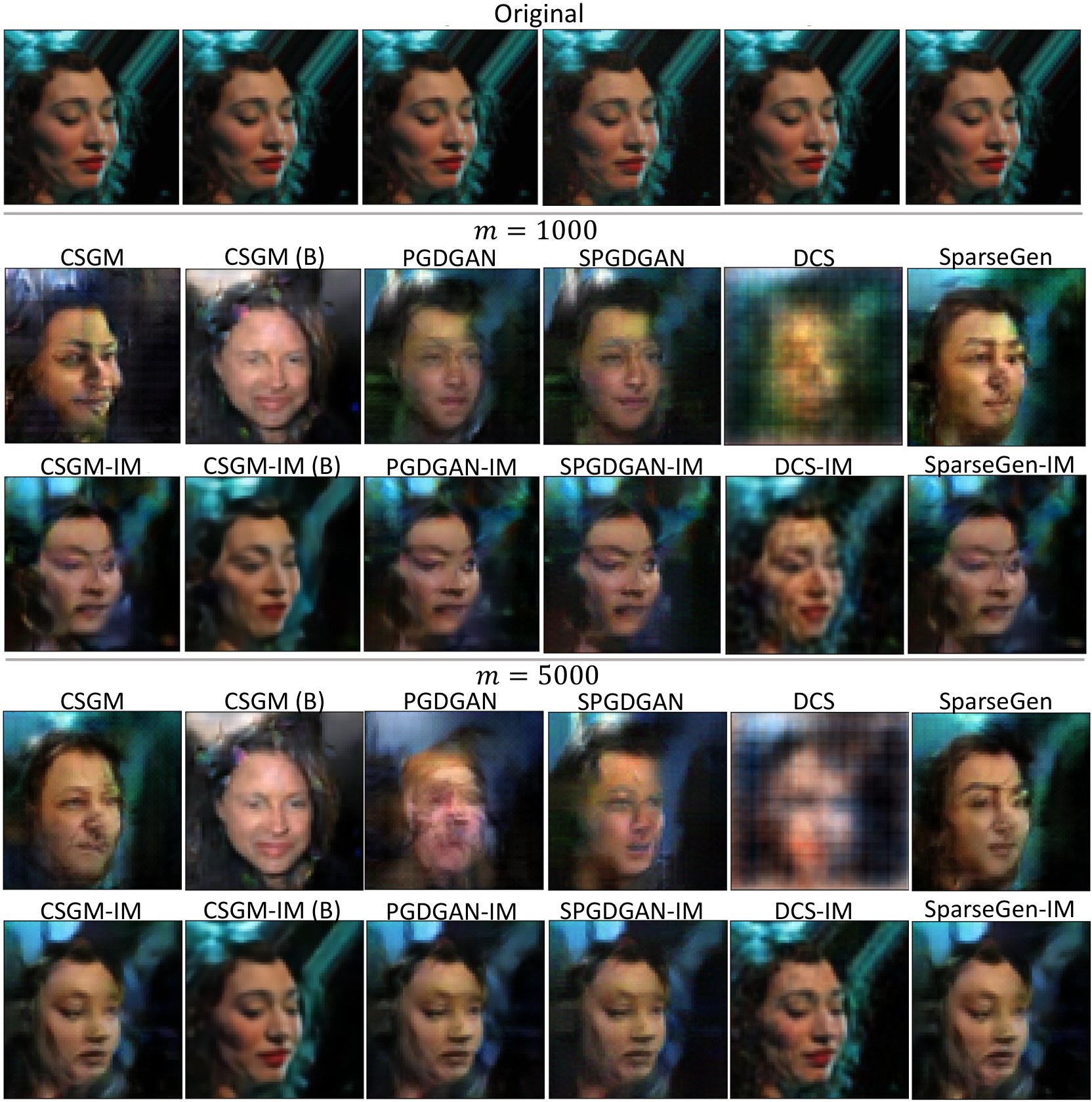
Figure 4: Reconstructed images on CelebA when m=1000​(m/d≈8.14%)m=1000\,\,(m/d\approx 8.14\%) and m=5000​(m/d≈40.69%)m=5000\,\,(m/d\approx 40.69\%). The first row represents the original images. Note that the original image in the fourth column of each test sample is a ss-sparse vector in the wavelet basis when s=d/2s=d/2. The second and third row indicate images recovered by existing methods and existing methods + IM when m=1000m=1000. The fourth and last rows display images recovered by existing methods and existing methods + IM when m=5000m=5000.
Table 2: Reconstruction error per pixel with 95%95\% confidence interval of 55 trials for existing methods and those with the IM framework. DCGAN is employed unless “B” is marked, where “B” stands for the use of BEGAN.
Method m=20m=20 m=100m=100 m=500m=500 m=1000m=1000 m=5000m=5000
CSGM [6] 0.304±0.0680.304\pm 0.068 0.104±0.0120.104\pm 0.012 0.039±0.0040.039\pm 0.004 0.033±0.0030.033\pm 0.003 0.029±0.0030.029\pm 0.003
CSGM-IM 0.209±0.011\mathbf{0.209\pm 0.011} 0.072±0.007\mathbf{0.072\pm 0.007} 0.029±0.003\mathbf{0.029\pm 0.003} 0.022±0.003\mathbf{0.022\pm 0.003} 0.018±0.002\mathbf{0.018\pm 0.002}
CSGM (B) 0.213±0.0310.213\pm 0.031 0.104±0.0120.104\pm 0.012 0.071±0.0110.071\pm 0.011 0.068±0.0100.068\pm 0.010 0.066±0.0110.066\pm 0.011
CSGM-IM (B) 0.185±0.008\mathbf{0.185\pm 0.008} 0.058±0.007\mathbf{0.058\pm 0.007} 0.015±0.002\mathbf{0.015\pm 0.002} 0.008±0.001\mathbf{0.008\pm 0.001} 0.002±0.000\mathbf{0.002\pm 0.000}
PGDGAN [19] 0.630±0.0760.630\pm 0.076 0.128±0.0100.128\pm 0.010 0.049±0.0060.049\pm 0.006 0.038±0.0040.038\pm 0.004 0.032±0.0040.032\pm 0.004
PGDGAN-IM 0.438±0.017\mathbf{0.438\pm 0.017} 0.094±0.007\mathbf{0.094\pm 0.007} 0.031±0.003\mathbf{0.031\pm 0.003} 0.023±0.003\mathbf{0.023\pm 0.003} 0.019±0.002\mathbf{0.019\pm 0.002}
SPGDGAN (Ours) 0.624±0.1100.624\pm 0.110 0.124±0.0100.124\pm 0.010 0.048±0.0050.048\pm 0.005 0.039±0.0040.039\pm 0.004 0.032±0.0040.032\pm 0.004
SPGDGAN-IM 0.425±0.021\mathbf{0.425\pm 0.021} 0.090±0.008\mathbf{0.090\pm 0.008} 0.031±0.003\mathbf{0.031\pm 0.003} 0.024±0.002\mathbf{0.024\pm 0.002} 0.020±0.002\mathbf{0.020\pm 0.002}
DCS [16] 0.246±0.0050.246\pm 0.005 0.159±0.0070.159\pm 0.007 0.114±0.0070.114\pm 0.007 0.087±0.0030.087\pm 0.003 0.082±0.0020.082\pm 0.002
DCS-IM 0.110±0.008\mathbf{0.110\pm 0.008} 0.049±0.005\mathbf{0.049\pm 0.005} 0.017±0.002\mathbf{0.017\pm 0.002} 0.010±0.001\mathbf{0.010\pm 0.001} 0.002±0.000\mathbf{0.002\pm 0.000}
SparseGen [10] 0.374±0.0600.374\pm 0.060 0.118±0.0180.118\pm 0.018 0.038±0.0050.038\pm 0.005 0.030±0.0040.030\pm 0.004 0.024±0.0030.024\pm 0.003
SparseGen-IM 0.224±0.022\mathbf{0.224\pm 0.022} 0.072±0.005\mathbf{0.072\pm 0.005} 0.028±0.003\mathbf{0.028\pm 0.003} 0.021±0.002\mathbf{0.021\pm 0.002} 0.017±0.002\mathbf{0.017\pm 0.002}

6 Experiments

6.1 Comparison to Existing CSPGs

In order to evaluate the effectiveness of our algorithm, we focus on conducting experiments on CelebA [41] dataset, which is a common but more difficult task than on MNIST [42] or OMNIGLOT [43]. The images are cropped at the center to the size 64×64×3​(d=12288)64\times 64\times 3\,(d=12288) and normalized into the range [−1,1][-1,1]. For inference, we utilize 64 random images in the test set and compute the reconstruction error ‖𝒙t​e−𝒙^‖2\left\lVert\boldsymbol{x}_{te}-\hat{\boldsymbol{x}}\right\rVert^{2} with 95%95\% confidence interval of 55 trials. Each entry of 𝑨\boldsymbol{A} is sampled from the normal distribution 𝒩⁡(0,1/m)\mathcal{N}(0,1/m).

When adding 𝒚\boldsymbol{y} into generative models, 𝒚\boldsymbol{y} is concatenated to 𝒛\boldsymbol{z} in G𝜽G_{\boldsymbol{\theta}} in both DCGAN and BEGAN. 𝒚\boldsymbol{y} is also concatenated to the embedding layer in DϕD_{\boldsymbol{\phi}} in BEGAN. Owing to the absence of an embedding layer in DϕD_{\boldsymbol{\phi}} in DCGAN, we emulate an architecture in Reed et al. 2016. The dimension of 𝒛\boldsymbol{z} is set to 100100 in DCGAN and 6464 in BEGAN, respectively. Further information about experimental settings and more experiments on different mm are postponed to Appendix.

CSGM-IM

As illustrated in Table 2, IM decreases the reconstruction error per pixel of CSGM by above 30%30\% on average , but CSGM-IM still exhibits performance saturation like CSGM. When exploiting BEGAN instead of DCGAN, however, CSGM-IM achieves better performance as well as overcomes such a limitation. Remarkably, for m≥1000m\geq 1000, the reconstruction error per pixel of CSGM-IM using BEGAN is almost less than that of CSGM using BEGAN by an order of magnitude, which makes CSGM-IM using BEGAN reconstruct images similar to the original ones as shown in Figure 4.

PGDGAN-IM

For fair comparisons, we use the same hyperparameters as Shah and Hegde 2018. In Table 2, IM reduces the reconstruction error per pixel of PGDGAN by above 30%30\% overall.

SPGDGAN-IM

Following Shah and Hegde 2018, SPGDGAN and SPGDGAN-IM with s=d/2s=d/2 are on par with PGDGAN and PGDGAN-IM respectively despite the presence of a sparsity operator.

DCS-IM

To verify the validness of our method in the absence of DϕD_{\boldsymbol{\phi}}, we apply IM to DCS. Table 2 shows that IM lowers the reconstruction error per pixel of DCS by above 70%70\% on average and by an order of magnitude for m≥1000m\geq 1000, which leads to successful signal recovery like CSGM-IM using BEGAN in Figure 4. More noticeably, DCS-IM outperforms all the other methods when m≤100m\leq 100.

SparseGen-IM

We only consider the wavelet basis due to the fact that Dhar et al. 2018 recommend the wavelet basis rather than the discrete cosine transform. Table 2 indicates that SparseGen-IM surpasses SparseGen, averagely curtailing the reconstruction error by around 38%38\%.

6.2 Ablation Studies

To figure out whether the improvement of IM merely results from the increased number of weights in the generator of CSGM-IM or not, we examine the case when the dimension of 𝒛\boldsymbol{z} in CSGM equals the sum of mm and that in CSGM-IM so as to make the number of weights in the generator of CSGM the same as that in the generator of CSGM-IM. In other words, d𝒛CSGM=m+d𝒛CSGM-IMd_{\boldsymbol{z}_{\text{CSGM}}}=m+d_{\boldsymbol{z}_{\text{CSGM-IM}}}, where d𝒛CSGMd_{\boldsymbol{z}_{\text{CSGM}}} and d𝒛CSGM-IMd_{\boldsymbol{z}_{\text{CSGM-IM}}} are the dimension of 𝒛CSGM\boldsymbol{z}_{\text{CSGM}}, 𝒛\boldsymbol{z} in CSGM, and that of 𝒛CSGM-IM\boldsymbol{z}_{\text{CSGM-IM}}, 𝒛\boldsymbol{z} in CSGM-IM. Here, we let d𝒛CSGM-IMd_{\boldsymbol{z}_{\text{CSGM-IM}}} equal mm to balance them. Table 4 shows there is still performance gap for every mm even if the generator of CSGM has the same number of weights as that of CSGM-IM. Moreover, the latent optimization performs well in CSGM-IM as seen in Figures 5(a) and 5(b).

Table 3: Reconstruction error per pixel with 95%95\% confidence interval of 55 trials for Section 4.1, where the number of weights in the generator of CSGM equals that in the generator of CSGM-IM and d𝒛CSGM-IMd_{\boldsymbol{z}_{\text{CSGM-IM}}} equals mm.
mm CSGM CSGM-IM
100100 0.103±0.0140.103\pm 0.014 0.072±0.007\mathbf{0.072\pm 0.007}
500500 0.029±0.0030.029\pm 0.003 0.019±0.002\mathbf{0.019\pm 0.002}
25002500 0.018±0.0020.018\pm 0.002 0.005±0.000\mathbf{0.005\pm 0.000}
Table 4: Reconstruction error per pixel with 95%95\% confidence interval of 55 trials for Section 4.1, where the number of weights in generator of CSGM equals that in generator of CSGM-IM with m=500m=500 and d𝒛CSGM-IMd_{\boldsymbol{z}_{\text{CSGM-IM}}} varies.
d𝒛CSGM-IMd_{\boldsymbol{z}_{\text{CSGM-IM}}} CSGM CSGM-IM
100100 0.030±0.0040.030\pm 0.004 0.028±0.003\mathbf{0.028\pm 0.003}
500500 0.029±0.0030.029\pm 0.003 0.019±0.003\mathbf{0.019\pm 0.003}
25002500 0.031±0.0070.031\pm 0.007 0.019±0.003\mathbf{0.019\pm 0.003}
(a) m=100m=100
(b) m=2500m=2500
(c) d𝒛CSGM-IM=100d_{\boldsymbol{z}_{\text{CSGM-IM}}}=100
(d) d𝒛CSGM-IM=2500d_{\boldsymbol{z}_{\text{CSGM-IM}}}=2500
Figure 5: Test phases of CSGM (the blue curve) and CSGM-IM (the red curve) – (a) and (b) for results in Table 4, (c) and (d) for results in Table 4.

To verify the superiority of CSGM-IM to CSGM when the ratio of mm to d𝒛CSGM-IMd_{\boldsymbol{z}_{\text{CSGM-IM}}} varies but still d𝒛CSGM=m+d𝒛CSGM-IMd_{\boldsymbol{z}_{\text{CSGM}}}=m+d_{\boldsymbol{z}_{\text{CSGM-IM}}}, we conduct experiments on different d𝒛CSGM-IMd_{\boldsymbol{z}_{\text{CSGM-IM}}} with mm fixed to 500500. As seen in Table 4 and Figures 5(c) and 5(d), CSGM-IM surpasses CSGM as well as the latent optimization works well in CSGM-IM no matter how small or large d𝒛CSGM-IMd_{\boldsymbol{z}_{\text{CSGM-IM}}} is. Hence, the direct insertion of 𝒚\boldsymbol{y} into generators plays a vital role in performance enhancement.

7 Application to Magnetic Resonance Imaging

In this section, we run experiments on knee data in fastMRI [44] to validate the practicality of IM on real-world data. Owing to the low quality of test slices, we utilize 6464 random images in the validation slices for inference. Unlike (1), noise is not added when creating a measurement vector. In this experiment, we solely employ BEGAN due to the fact that it works best among our experiments. The details of the experimental setup are deferred to Appendix.

Similarly to Section 6.1, CSGM-IM outdoes CSGM as seen in Table 5. For m≥2500m\geq 2500, IM lowers the reconstruction error of CSGM by closely an order of magnitude. Not only that, as shown in Figure 6, CSGM-IM recovers images highly analogous to the original ones whereas CSGM cannot at all.

8 Conclusion

Table 5: MRI reconstruction error per pixel with 95%95\% confidence interval of 55 trials for Section 4.1 with BEGAN.
mm CSGM (B) CSGM-IM (B)
500500 0.0674±0.01180.0674\pm 0.0118 0.0159±0.0007\mathbf{0.0159\pm 0.0007}
10001000 0.0671±0.00970.0671\pm 0.0097 0.0120±0.0007\mathbf{0.0120\pm 0.0007}
25002500 0.0655±0.01010.0655\pm 0.0101 0.0092±0.0005\mathbf{0.0092\pm 0.0005}
50005000 0.0659±0.01230.0659\pm 0.0123 0.0082±0.0005\mathbf{0.0082\pm 0.0005}
Refer to caption
(a) The 193193rd validation slice
Refer to caption
(b) The 928928th validation slice
Figure 6: Reconstructed images on fastMRI when m=5000​(m/d≈30.52%)m=5000\,(m/d\approx 30.52\%). The first column has the original image. The second and last column show images recovered by CSGM and CSGM-IM using BEGAN.

We propose a simple yet effective method, Inserting Measurements, which allows a generator to exploit 𝒚\boldsymbol{y} in both of training and test phases, where existing generative models are limited to use 𝒚\boldsymbol{y} only in the test phase. Even in the IM framework, the characteristic of generative models remains, which allows us to find a more closer estimate to the true signal by the latent optimization. By leveraging both advantages of discriminative and generative models, IM can yield much smaller reconstruction error than existing methods up to an order of magnitude. We therefore expect IM to be useful for a variety of CS applications as well as image recovery.

References

  • He et al. [2018] Hengtao He, Chao-Kai Wen, Shi Jin, and Geoffrey Ye Li. Deep learning-based channel estimation for beamspace mmWave massive MIMO systems. IEEE Wireless Communications Letters, 7(5):852–855, 2018.
  • Kim and Chung [2020] Kyung-Su Kim and Sae-Young Chung. Tree search network for sparse estimation. Digital Signal Processing, 100:102680, 02 2020. doi: 10.1016/j.dsp.2020.102680.
  • Lustig et al. [2007] Michael Lustig, David L. Donoho, Juan M. Santos, and John M. Pauly. Compressed sensing MRI. In IEEE Signal Processing Magazine, 2007.
  • Sun et al. [2016] Jian Sun, Huibin Li, Zongben Xu, et al. Deep ADMM-Net for compressive sensing MRI. In Advances in Neural Information Processing Systems, pages 10–18, 2016.
  • Willett et al. [2011] Rebecca M Willett, Roummel F Marcia, and Jonathan M Nichols. Compressed sensing for practical optical imaging systems: a tutorial. Optical Engineering, 50(7):072601, 2011.
  • Bora et al. [2017] Ashish Bora, Ajil Jalal, Eric Price, and Alexandros G Dimakis. Compressed sensing using generative models. In International Conference on Machine Learning, pages 537–546. JMLR. org, 2017.
  • He et al. [2017] Hao He, Bo Xin, Satoshi Ikehata, and David Wipf. From Bayesian sparsity to gated recurrent nets. In Advances in Neural Information Processing Systems, pages 5554–5564, 2017.
  • Metzler et al. [2017] Chris Metzler, Ali Mousavi, and Richard Baraniuk. Learned D-AMP: Principled neural network based compressive image recovery. In Advances in Neural Information Processing Systems, pages 1772–1783, 2017.
  • Van Veen et al. [2018] Dave Van Veen, Ajil Jalal, Mahdi Soltanolkotabi, Eric Price, Sriram Vishwanath, and Alexandros G Dimakis. Compressed sensing with deep image prior and learned regularization. arXiv preprint:1806.06438, 2018.
  • Dhar et al. [2018] Manik Dhar, Aditya Grover, and Stefano Ermon. Modeling sparse deviations for compressed sensing using generative models. In International Conference on Machine Learning, pages 1222–1231, 2018.
  • Mardani et al. [2018] Morteza Mardani, Qingyun Sun, David Donoho, Vardan Papyan, Hatef Monajemi, Shreyas Vasanawala, and John Pauly. Neural proximal gradient descent for compressive imaging. In Advances in Neural Information Processing Systems, pages 9573–9583, 2018.
  • Lunz et al. [2018] Sebastian Lunz, Ozan Öktem, and Carola-Bibiane Schönlieb. Adversarial regularizers in inverse problems. In Advances in Neural Information Processing Systems, pages 8507–8516, 2018.
  • Mousavi et al. [2019] Ali Mousavi, Gautam Dasarathy, and Richard G Baraniuk. A data-driven and distributed approach to sparse signal representation and recovery. In International Conference on Learning Representations, 2019.
  • Grover and Ermon [2019] Aditya Grover and Stefano Ermon. Uncertainty autoencoders: Learning compressed representations via variational information maximization. In International Conference on Artificial Intelligence and Statistics, pages 2514–2524, 2019.
  • Wu et al. [2019a] Shanshan Wu, Alexandros Dimakis, Sujay Sanghavi, Felix Yu, Daniel Holtmann-Rice, Dmitry Storcheus, Afshin Rostamizadeh, and Sanjiv Kumar. Learning a compressed sensing measurement matrix via gradient unrolling. In International Conference on Machine Learning, volume 97, 2019a.
  • Wu et al. [2019b] Yan Wu, Mihaela Rosca, and Timothy Lillicrap. Deep compressed sensing. In International Conference on Machine Learning, pages 6850–6860, 2019b.
  • Raj et al. [2019] Ankit Raj, Yuqi Li, and Yoram Bresler. GAN-based projector for faster recovery with convergence guarantees in linear inverse problems. In IEEE/CVF International Conference on Computer Vision, pages 5601–5610, 2019.
  • Tibshirani [1996] Robert Tibshirani. Regression shrinkage and selection via the LASSO. Journal of the Royal Statistical Society: Series B (Methodological), 58(1):267–288, 1996.
  • Shah and Hegde [2018] Viraj Shah and Chinmay Hegde. Solving linear inverse problems using GAN priors: An algorithm with provable guarantees. In IEEE International Conference on Acoustics, Speech and Signal Processing, pages 4609–4613. IEEE, 2018.
  • Kabkab et al. [2018] Maya Kabkab, Pouya Samangouei, and Rama Chellappa. Task-aware compressed sensing with generative adversarial networks. In AAAI Conference on Artificial Intelligence, 2018.
  • Gregor and LeCun [2010] Karol Gregor and Yann LeCun. Learning fast approximations of sparse coding. In International Conference on Machine Learning, pages 399–406, 2010.
  • Moreau and Bruna [2017] Thomas Moreau and Joan Bruna. Understanding neural sparse coding with matrix factorization. In International Conference on Learning Representations, 2017.
  • Giryes et al. [2018] Raja Giryes, Yonina C Eldar, Alex M Bronstein, and Guillermo Sapiro. Tradeoffs between convergence speed and reconstruction accuracy in inverse problems. IEEE Transactions on Signal Processing, 66(7):1676–1690, 2018.
  • Chen et al. [2018] Xiaohan Chen, Jialin Liu, Zhangyang Wang, and Wotao Yin. Theoretical linear convergence of unfolded ISTA and its practical weights and thresholds. In Advances in Neural Information Processing Systems, pages 9061–9071, 2018.
  • Tramel et al. [2016] Eric W Tramel, Angélique Drémeau, and Florent Krzakala. Approximate message passing with restricted Boltzmann machine priors. Journal of Statistical Mechanics: Theory and Experiment, 2016(7):073401, 2016.
  • Borgerding et al. [2017] Mark Borgerding, Philip Schniter, and Sundeep Rangan. AMP-inspired deep networks for sparse linear inverse problems. IEEE Transactions on Signal Processing, 65(16):4293–4308, 2017.
  • Jagatap and Hegde [2019] G Jagatap and C Hegde. Algorithmic guarantees for inverse imaging with untrained network priors. In Advances in Neural Information Processing Systems, 2019.
  • Ulyanov et al. [2018] Dmitry Ulyanov, Andrea Vedaldi, and Victor Lempitsky. Deep image prior. In IEEE/CVF Conference on Computer Vision and Pattern Recognition, pages 9446–9454, 2018.
  • Heckel et al. [2019] R Heckel et al. Deep decoder: Concise image representations from untrained non-convolutional networks. In International Conference on Learning Representations, 2019.
  • Mirza and Osindero [2014] Mehdi Mirza and Simon Osindero. Conditional generative adversarial nets. arXiv preprint:1411.1784, 2014.
  • Reed et al. [2016] Scott Reed, Zeynep Akata, Xinchen Yan, Lajanugen Logeswaran, Bernt Schiele, and Honglak Lee. Generative adversarial text to image synthesis. In International Conference on Machine Learning, pages 1060–1069, 2016.
  • Isola et al. [2017] Phillip Isola, Jun-Yan Zhu, Tinghui Zhou, and Alexei A Efros. Image-to-image translation with conditional adversarial networks. In Proceedings of the IEEE Conference on Computer Vision and Pattern Recognition, pages 1125–1134, 2017.
  • Wang et al. [2018] Ting-Chun Wang, Ming-Yu Liu, Jun-Yan Zhu, Andrew Tao, Jan Kautz, and Bryan Catanzaro. High-resolution image synthesis and semantic manipulation with conditional GANs. In Proceedings of the IEEE Conference on Computer Vision and Pattern Recognition, pages 8798–8807, 2018.
  • Uelwer et al. [2019] Tobias Uelwer, Alexander Oberstraß, and Stefan Harmeling. Phase retrieval using conditional generative adversarial networks. arXiv preprint:1912.04981, 2019.
  • Ye et al. [2020] Hao Ye, Le Liang, Geoffrey Ye Li, and Biing-Hwang Juang. Deep learning based end-to-end wireless communication systems with conditional GAN as unknown channel. IEEE Transactions on Wireless Communications, 2020.
  • Goodfellow et al. [2014] Ian Goodfellow, Jean Pouget-Abadie, Mehdi Mirza, Bing Xu, David Warde-Farley, Sherjil Ozair, Aaron Courville, and Yoshua Bengio. Generative adversarial nets. In Advances in Neural Information Processing Systems, pages 2672–2680, 2014.
  • Radford et al. [2015] Alec Radford, Luke Metz, and Soumith Chintala. Unsupervised representation learning with deep convolutional generative adversarial networks. arXiv preprint:1511.06434, 2015.
  • Kingma and Welling [2014] Diederik P. Kingma and Max Welling. Auto-encoding variational Bayes. In International Conference on Learning Representations, 2014.
  • Maaten and Hinton [2008] Laurens van der Maaten and Geoffrey Hinton. Visualizing data using t-sne. Journal of machine learning research, 9(Nov):2579–2605, 2008.
  • Lee et al. [2012] Kiryung Lee, Yoram Bresler, and Marius Junge. Subspace methods for joint sparse recovery. IEEE Transactions on Information Theory, 58(6):3613–3641, 2012.
  • Liu et al. [2015] Ziwei Liu, Ping Luo, Xiaogang Wang, and Xiaoou Tang. Deep learning face attributes in the wild. In Proceedings of International Conference on Computer Vision, December 2015.
  • LeCun et al. [1998] Yann LeCun, Léon Bottou, Yoshua Bengio, and Patrick Haffner. Gradient-based learning applied to document recognition. Proceedings of the IEEE, 86(11):2278–2324, 1998.
  • Lake et al. [2015] Brenden M. Lake, Ruslan Salakhutdinov, and Joshua B. Tenenbaum. Human-level concept learning through probabilistic program induction. Science, 350:1332–1338, 2015.
  • Zbontar et al. [2018] Jure Zbontar, Florian Knoll, Anuroop Sriram, Matthew J Muckley, Mary Bruno, Aaron Defazio, Marc Parente, Krzysztof J Geras, Joe Katsnelson, Hersh Chandarana, et al. FastMRI: An open dataset and benchmarks for accelerated MRI. arXiv preprint:1811.08839, 2018.
  • Finn et al. [2017] Chelsea Finn, Pieter Abbeel, and Sergey Levine. Model-agnostic meta-learning for fast adaptation of deep networks. In International Conference on Machine Learning, volume 70, pages 1126–1135. PMLR, 2017.
  • Davidson and Szarek [2001] Kenneth R Davidson and Stanislaw J Szarek. Local operator theory, random matrices and banach spaces. Handbook of the geometry of Banach spaces, 1(317-366):131, 2001.

Appendix A Additional Implementations

A.1 Deep Compressed Sensing (DCS)

DCS

To recover signals faster and more accurately than CSGM, Wu et al. 2019b proposed Deep Compressed Sensing (DCS) by jointly training the latent variables 𝒛\boldsymbol{z} and the weights 𝜽\boldsymbol{\theta} of a generator without any discriminator DϕD_{\phi} via meta-learning [45]. More concretely, the training phase of DCS is given as follows: for each training sample 𝒙t​r\boldsymbol{x}_{tr}, the latent optimization is carried out by minimizing ‖𝒚t​r−𝑨​G𝜽​(𝒛)‖\left\|\boldsymbol{y}_{tr}-\boldsymbol{A}G_{\boldsymbol{\theta}}(\boldsymbol{z})\right\| while keeping 𝜽\boldsymbol{\theta} fixed, then 𝜽\boldsymbol{\theta} are subsequently trained in DCS:

𝒛𝒙t​r∗=arg⁡min𝒛​‖𝒚t​r−𝑨​G𝜽​(𝒛)‖,\displaystyle\boldsymbol{z}^{*}_{\boldsymbol{x}_{tr}}=\underset{\boldsymbol{z}}{\arg\min}\left\|\boldsymbol{y}_{tr}-\boldsymbol{A}G_{\boldsymbol{\theta}}(\boldsymbol{z})\right\|, (18)
𝜽∗=ℱ𝜽o​p​t​[ℒt​r​(G𝜽​(𝒛𝒙t​r∗))]=arg⁡min𝜽​𝔼𝒙t​r∼p⁡(𝒙)​[‖𝒚t​r−𝑨​G𝜽​(𝒛𝒙t​r∗)‖2].\displaystyle\boldsymbol{\theta}^{*}=\mathcal{F}^{opt}_{\boldsymbol{\theta}}\Big[\mathcal{L}_{tr}\big(G_{\boldsymbol{\theta}}(\boldsymbol{z}^{*}_{\boldsymbol{x}_{tr}})\big)\Big]=\underset{\boldsymbol{\theta}}{\arg\min}\,\mathbb{E}_{\boldsymbol{x}_{tr}\sim p(\boldsymbol{x})}\Big[\left\|\boldsymbol{y}_{tr}-\boldsymbol{A}G_{\boldsymbol{\theta}}(\boldsymbol{z}^{*}_{\boldsymbol{x}_{tr}})\right\|^{2}\Big]. (19)

Note that the test phase of DCS is the same as that of CSGM (8), so it is not shown here.

DCS-IM

Similarly to (9) and (10), the IM framework makes the measurement information also taken by GθG_{\theta} as additional input in DCS. Therefore, by applying IM to DCS, (18) and (19), the procedure for training 𝜽\boldsymbol{\theta}, are substituted with (20) and (21), respectively.

𝒛𝒙t​r∗\displaystyle\boldsymbol{z}^{*}_{\boldsymbol{x}_{tr}} =arg⁡min𝒛​‖𝒚t​r−𝑨​G𝜽​(𝒛,𝒚t​r)‖,\displaystyle=\underset{\boldsymbol{z}}{\arg\min}\left\|\boldsymbol{y}_{tr}-\boldsymbol{A}G_{\boldsymbol{\theta}}(\boldsymbol{z},\color[rgb]{0,0,0}\boldsymbol{y}_{tr})\right\|, (20)
𝜽∗\displaystyle\boldsymbol{\theta}^{*} =ℱ𝜽o​p​t​[ℒt​r​(G𝜽​(𝒛𝒙t​r∗,𝒚t​r))]=arg⁡min𝜽​𝔼𝒙t​r∼p⁡(𝒙)​[‖𝒚t​r−𝑨​G𝜽​(𝒛𝒙t​r∗,𝒚t​r)‖2].\displaystyle=\mathcal{F}^{opt}_{\boldsymbol{\theta}}\Big[\mathcal{L}_{tr}\big(G_{\boldsymbol{\theta}}(\boldsymbol{z}^{*}_{\boldsymbol{x}_{tr}},{\color[rgb]{0,0,0}\boldsymbol{y}_{tr}})\big)\Big]=\underset{\boldsymbol{\theta}}{\arg\min}\,\mathbb{E}_{\boldsymbol{x}_{tr}\sim p(\boldsymbol{x})}\Big[\left\|\boldsymbol{y}_{tr}-\boldsymbol{A}G_{\boldsymbol{\theta}}(\boldsymbol{z}^{*}_{\boldsymbol{x}_{tr}},\color[rgb]{0,0,0}\boldsymbol{y}_{tr})\right\|^{2}\Big]. (21)

As the formula of DCS in the test phase is the same as that of CSGM (8), the formula of DCS with the IM framework is also identical to that of CSGM-IM (11), but notice that a couple of gradient descent steps are sufficient to implement (8) in DCS and (11) in DCS with the IM framework.

In such a case of applying IM to DCS in the training and test phases, we name it DCS-IM. The algorithms of DCS and DCS-IM are given in Section D.

A.2 Sparse deviations for compressed sensing using Generative models (SparseGen)

SparseGen

Dhar et al. 2018 came up with the idea to combine a domain-specific generative model prior with sparsity prior to enhance the generalization of CSGM, called SparseGen. Similarly to CSGM, the training phase of SparseGen can be any learning scheme to optimize a generator G𝜽G_{\boldsymbol{\theta}} like (6) or (7). In the test phase of SparseGen, given trained parameters 𝜽∗\boldsymbol{\theta}^{*} of a generator, sparse deviations from the support set of G𝜽∗G_{\boldsymbol{\theta}^{*}} are allowed to consider signals even outside the range of G𝜽∗G_{\boldsymbol{\theta}^{*}}, which results in an estimate being of the form G𝜽∗+𝝂G_{\boldsymbol{\theta}^{*}}+\boldsymbol{\nu} where 𝝂\boldsymbol{\nu} is an augmented sparse estimate. Hence, ℒt​e\mathcal{L}_{te} should be involved with ℓ1\ell_{1} minimization with respect to 𝝂\boldsymbol{\nu} as well as the optimization of G𝜽∗G_{\boldsymbol{\theta}^{*}} with respect to 𝒛\boldsymbol{z}:

(𝒛∗,𝝂∗)=ℱ(𝒛,𝝂)o​p​t​[ℒt​e​(G𝜽∗​(𝒛),𝝂|𝒚t​e)]=arg⁡min𝒛,𝝂​‖𝑨⁡(G𝜽∗​(𝒛)+𝝂)−𝒚t​e‖+λ​‖𝑩​𝝂‖1,\displaystyle(\boldsymbol{z}^{*},\boldsymbol{\nu}^{*})=\mathcal{F}^{opt}_{(\boldsymbol{z},\boldsymbol{\nu})}[\mathcal{L}_{te}(G_{\boldsymbol{\theta}^{*}}(\boldsymbol{z}),\boldsymbol{\nu}\,|\,\boldsymbol{y}_{te})]=\underset{\boldsymbol{z},\boldsymbol{\nu}}{\arg\min}\left\|\boldsymbol{A}(G_{{\boldsymbol{\theta}}^{*}}(\boldsymbol{z})+\boldsymbol{\nu})-\boldsymbol{y}_{te}\right\|+\lambda\left\|\boldsymbol{B}\boldsymbol{\nu}\right\|_{1}, (22)

where 𝑩\boldsymbol{B} is a transform matrix promoting sparsity of the vector 𝑩​𝝂\boldsymbol{B}\boldsymbol{\nu}, and λ\lambda is the Lagrange multiplier. By using (𝒛∗,𝝂∗)(\boldsymbol{z}^{*},\boldsymbol{\nu}^{*}) given in (22), SparseGen estimates the target signal as G𝜽∗​(𝒛∗)+𝝂∗G_{{\boldsymbol{\theta}}^{*}}(\boldsymbol{z}^{*})+\boldsymbol{\nu}^{*}.

SparseGen-IM

IM can be run on SparseGen by adjusting (22) to (23):

(𝒛∗,𝝂∗)=ℱ(𝒛,𝝂)o​p​t​[ℒt​e​(G𝜽∗​(𝒛,𝒚t​e),𝝂|𝒚t​e)]=arg⁡min𝒛,𝝂​‖𝑨⁡(G𝜽∗​(𝒛,𝒚t​e)+𝝂)−𝒚t​e‖+λ​‖𝑩​𝝂‖1,\displaystyle(\boldsymbol{z}^{*},\boldsymbol{\nu}^{*})=\mathcal{F}^{opt}_{(\boldsymbol{z},\boldsymbol{\nu})}[\mathcal{L}_{te}(G_{\boldsymbol{\theta}^{*}}(\boldsymbol{z},{\color[rgb]{0,0,0}\boldsymbol{y}_{te}}),\boldsymbol{\nu}\,|\,\boldsymbol{y}_{te})]=\underset{\boldsymbol{z},\boldsymbol{\nu}}{\arg\min}\left\|\boldsymbol{A}(G_{{\boldsymbol{\theta}}^{*}}(\boldsymbol{z},{\color[rgb]{0,0,0}\boldsymbol{y}_{te}})+\boldsymbol{\nu})-\boldsymbol{y}_{te}\right\|+\lambda\left\|\boldsymbol{B}\boldsymbol{\nu}\right\|_{1}, (23)

which we name SparseGen-IM. In this case, G𝜽∗​(𝒛∗,𝒚t​e)+𝝂∗G_{{\boldsymbol{\theta}}^{*}}(\boldsymbol{z}^{*},\boldsymbol{y}_{te})+\boldsymbol{\nu}^{*} becomes an estimate of 𝒙t​e\boldsymbol{x}_{te}. As SparseGen has the same training phase as CSGM, SparseGen-IM also has the same training phase as CSGM-IM ((9) or (10)).

The algorithms of SparseGen and SparseGen-IM are given in Section D.

Appendix B Proof of Theorem 1

The proof of Theorem 1 is based on that of Theorem 1 in Jagatap and Hegde 2019.

Let the following algorithm be the test phase of SPGDGAN (without blue notes) and SPGDGAN-IM (with blue notes) in the noiseless setting, 𝒚=𝑨​𝒙\boldsymbol{y}=\boldsymbol{A}\boldsymbol{x}.

1: 𝒚t​e∈ℝm,𝑨∈ℝm×d\boldsymbol{y}_{te}\in\mathbb{R}^{m},\boldsymbol{A}\in\mathbb{R}^{m\times d}, G𝜽∗:ℝv↦ℝdG_{{\boldsymbol{\theta}}^{*}}:\mathbb{R}^{v}\mapsto\mathbb{R}^{d}, α∈ℝ+\alpha\in\mathbb{R}_{+}, T∈ℕT\in\mathbb{N}
2: 𝒙0=𝟎∈ℝd\boldsymbol{x}_{0}=\boldsymbol{0}\in\mathbb{R}^{d}
3: for t=0t=0 to T−1T-1 do
4:   𝒘t=𝒙t−α​𝑨⊤​(𝑨​𝒙t−𝒚t​e)\boldsymbol{w}_{t}=\boldsymbol{x}_{t}-\alpha\boldsymbol{A}^{\top}(\boldsymbol{A}\boldsymbol{x}_{t}-\boldsymbol{y}_{te})
5:   𝒛t=argmin𝒛‖𝒘t−G𝜽∗​(𝒛,𝒚t​e)‖\boldsymbol{z}_{t}=\operatornamewithlimits{argmin}\limits_{\boldsymbol{z}}\left\|\boldsymbol{w}_{t}-G_{\boldsymbol{\theta}^{*}}(\boldsymbol{z},\color[rgb]{0,0,1}\boldsymbol{y}_{te})\right\|
6:   𝒙t+1=𝑼​hs​(𝑼⊤​G𝜽∗​(𝒛t,𝒚t​e))\boldsymbol{x}_{t+1}=\boldsymbol{U}h_{s}\Big(\boldsymbol{U}^{\top}G_{\boldsymbol{\theta}^{*}}\big(\boldsymbol{z}_{t},\color[rgb]{0,0,1}\boldsymbol{y}_{te}\big)\Big)
7: end for
8: the signal estimate 𝒙^=𝒙T\hat{\boldsymbol{x}}=\boldsymbol{x}_{T}

Referring to the above algorithm, we prove Theorem 1 under the condition (b) (i.e., the guarantee of signal recovery in SPGDGAN-IM). The proof of Theorem 1 under the condition (a) (i.e., the guarantee of signal recovery in SPGDGAN) is trivial if we remove all the blue notes below and use the condition (a) instead of (b).

It follows that

‖𝒚t​e−𝑨​𝒙t+1‖2−‖𝒚t​e−𝑨​𝒙t‖2\displaystyle\left\|\boldsymbol{y}_{te}-\boldsymbol{A}\boldsymbol{x}_{t+1}\right\|^{2}-\left\|\boldsymbol{y}_{te}-\boldsymbol{A}\boldsymbol{x}_{t}\right\|^{2}
=(‖𝑨​𝒙t+1‖2−‖𝑨​𝒙t‖2)−2​(𝒚t​e⊤​𝑨​𝒙t+1−𝒚t​e⊤​𝑨​𝒙t)\displaystyle=(\left\|\boldsymbol{Ax}_{t+1}\right\|^{2}-\left\|\boldsymbol{Ax}_{t}\right\|^{2})-2(\boldsymbol{y}_{te}^{\top}\boldsymbol{Ax}_{t+1}-\boldsymbol{y}_{te}^{\top}\boldsymbol{Ax}_{t})
=‖𝑨​𝒙t+1−𝑨​𝒙t‖2−2​(𝑨​𝒙t)⊤​(𝑨​𝒙t)+2​(𝑨​𝒙t)⊤​(𝑨​𝒙t+1)−2​(𝒚t​e⊤​𝑨​𝒙t+1−𝒚t​e⊤​𝑨​𝒙t)\displaystyle=\left\|\boldsymbol{A}\boldsymbol{x}_{t+1}-\boldsymbol{A}\boldsymbol{x}_{t}\right\|^{2}-2(\boldsymbol{A}\boldsymbol{x}_{t})^{\top}(\boldsymbol{A}\boldsymbol{x}_{t})+2(\boldsymbol{A}\boldsymbol{x}_{t})^{\top}(\boldsymbol{A}\boldsymbol{x}_{t+1})-2(\boldsymbol{y}_{te}^{\top}\boldsymbol{A}\boldsymbol{x}_{t+1}-\boldsymbol{y}_{te}^{\top}\boldsymbol{A}\boldsymbol{x}_{t})
=‖𝑨​𝒙t+1−𝑨​𝒙t‖2+2​(𝑨​𝒙t−𝒚t​e)⊤​(𝑨​𝒙t+1−𝑨​𝒙t).\displaystyle=\left\|\boldsymbol{A}\boldsymbol{x}_{t+1}-\boldsymbol{A}\boldsymbol{x}_{t}\right\|^{2}+2(\boldsymbol{A}\boldsymbol{x}_{t}-\boldsymbol{y}_{te})^{\top}(\boldsymbol{A}\boldsymbol{x}_{t+1}-\boldsymbol{A}\boldsymbol{x}_{t}). (24)

Line 2 of the SPGDGAN-IM algorithm is given as

𝒘t=𝒙t−α​𝑨⊤​(𝑨​𝒙t−𝒚t​e).\displaystyle\boldsymbol{w}_{t}=\boldsymbol{x}_{t}-\alpha\boldsymbol{A}^{\top}(\boldsymbol{A}\boldsymbol{x}_{t}-\boldsymbol{y}_{te}). (25)

Afterward, by using 𝒘t\boldsymbol{w}_{t} in (25), line 3 of the SPGDGAN-IM algorithm updates the latent variables 𝒛\boldsymbol{z} so that G𝜽∗​(𝒛,𝒚t​e)G_{\boldsymbol{\theta}^{*}}(\boldsymbol{z},\color[rgb]{0,0,1}\boldsymbol{y}_{te}) lies in the range of the generator G𝜽∗G_{\boldsymbol{\theta}^{*}} while being the closest to 𝒘t\boldsymbol{w}_{t}.

From line 4 of the SPGDGAN algorithm, 𝑼​hs​(𝑼⊤​(G𝜽∗​(𝒛t,𝒚t​e)))=𝒙t+1\boldsymbol{U}h_{s}\Big(\boldsymbol{U}^{\top}\big(G_{\boldsymbol{\theta}^{*}}(\boldsymbol{z}_{t},{\color[rgb]{0,0,1}\boldsymbol{y}_{te}})\big)\Big)=\boldsymbol{x}_{t+1}. By the condition (b), there exists 𝒛∗\boldsymbol{z}^{*} satisfying G𝜽∗​(𝒛∗,𝒚t​e)=𝒙t​eG_{\boldsymbol{\theta}^{*}}(\boldsymbol{z}^{*},{\color[rgb]{0,0,1}\boldsymbol{y}_{te}})=\boldsymbol{x}_{te} so that 𝑼​hs​(𝑼⊤​(G𝜽∗​(𝒛∗,𝒚t​e)))=𝒙t​e\boldsymbol{U}h_{s}\Big(\boldsymbol{U}^{\top}\big(G_{\boldsymbol{\theta}^{*}}(\boldsymbol{z}^{*},{\color[rgb]{0,0,1}\boldsymbol{y}_{te}})\big)\Big)=\boldsymbol{x}_{te}. Then, by using these two results and the definition of 𝒛t\boldsymbol{z}_{t} in line 3, we obtain

‖𝒙t+1−𝒘t‖2≤‖𝒙t​e−𝒘t‖2.\displaystyle\left\|\boldsymbol{x}_{t+1}-\boldsymbol{w}_{t}\right\|^{2}\leq\left\|\boldsymbol{x}_{te}-\boldsymbol{w}_{t}\right\|^{2}. (26)

By applying (25) to (26), we obtain

‖𝒙t+1−𝒙t+α​𝑨⊤​(𝑨​𝒙t−𝒚t​e)‖2≤‖𝒙t​e−𝒙t+α​𝑨⊤​(𝑨​𝒙t−𝒚t​e)‖2.\displaystyle\left\|\boldsymbol{x}_{t+1}-\boldsymbol{x}_{t}+\alpha\boldsymbol{A}^{\top}(\boldsymbol{A}\boldsymbol{x}_{t}-\boldsymbol{y}_{te})\right\|^{2}\leq\left\|\boldsymbol{x}_{te}-\boldsymbol{x}_{t}+\alpha\boldsymbol{A}^{\top}(\boldsymbol{A}\boldsymbol{x}_{t}-\boldsymbol{y}_{te})\right\|^{2}. (27)

(27) can be written as

‖𝒙t+1−𝒙t‖2+2​α​‖(𝒙t+1−𝒙t)T​𝑨T​(𝑨​𝒙t−𝒚t​e)‖\displaystyle\left\|\boldsymbol{x}_{t+1}-\boldsymbol{x}_{t}\right\|^{2}+2\alpha\left\|(\boldsymbol{x}_{t+1}-\boldsymbol{x}_{t})^{T}\boldsymbol{A}^{T}(\boldsymbol{A}\boldsymbol{x}_{t}-\boldsymbol{y}_{te})\right\| ≤‖𝒙t​e−𝒙t‖2+2​α​‖(𝒙t​e−𝒙t)T​𝑨T​(𝑨​𝒙t−𝒚t​e)‖\displaystyle\leq\left\|\boldsymbol{x}_{te}-\boldsymbol{x}_{t}\right\|^{2}+2\alpha\left\|(\boldsymbol{x}_{te}-\boldsymbol{x}_{t})^{T}\boldsymbol{A}^{T}(\boldsymbol{A}\boldsymbol{x}_{t}-\boldsymbol{y}_{te})\right\|
=‖𝒙t​e−𝒙t‖2+2​α​‖(𝑨​𝒙t​e−𝑨​𝒙t)T​(𝑨​𝒙t−𝒚t​e)‖\displaystyle=\left\|\boldsymbol{x}_{te}-\boldsymbol{x}_{t}\right\|^{2}+2\alpha\left\|(\boldsymbol{A}\boldsymbol{x}_{te}-\boldsymbol{A}\boldsymbol{x}_{t})^{T}(\boldsymbol{A}\boldsymbol{x}_{t}-\boldsymbol{y}_{te})\right\|
=‖𝒙t​e−𝒙t‖2+2​α​‖(𝒚t​e−𝑨​𝒙t)T​(𝑨​𝒙t−𝒚t​e)‖\displaystyle=\left\|\boldsymbol{x}_{te}-\boldsymbol{x}_{t}\right\|^{2}+2\alpha\left\|(\boldsymbol{y}_{te}-\boldsymbol{A}\boldsymbol{x}_{t})^{T}(\boldsymbol{A}\boldsymbol{x}_{t}-\boldsymbol{y}_{te})\right\|
=‖𝒙t​e−𝒙t‖2−2​α​‖𝒚t​e−𝑨​𝒙t‖2.\displaystyle=\left\|\boldsymbol{x}_{te}-\boldsymbol{x}_{t}\right\|^{2}-2\alpha\left\|\boldsymbol{y}_{te}-\boldsymbol{A}\boldsymbol{x}_{t}\right\|^{2}.

By dividing both sides by α\alpha,

1α​‖𝒙t+1−𝒙t‖2+2​(𝑨​𝒙t−𝒚t​e)⊤​𝑨​(𝒙t+1−𝒙t)≤1α​‖𝒙t−𝒙t​e‖2−2​‖𝒚t​e−𝑨​𝒙t‖2.\displaystyle\frac{1}{\alpha}\left\|\boldsymbol{x}_{t+1}-\boldsymbol{x}_{t}\right\|^{2}+2(\boldsymbol{A}\boldsymbol{x}_{t}-\boldsymbol{y}_{te})^{\top}\boldsymbol{A}(\boldsymbol{x}_{t+1}-\boldsymbol{x}_{t})\leq\frac{1}{\alpha}\left\|\boldsymbol{x}_{t}-\boldsymbol{x}_{te}\right\|^{2}-2\left\|\boldsymbol{y}_{te}-\boldsymbol{A}\boldsymbol{x}_{t}\right\|^{2}. (28)

Then, by applying (24) to (28), we gain

‖𝒚t​e−𝑨​𝒙t+1‖2+‖𝒚t​e−𝑨​𝒙t‖2≤1α​‖𝒙t−𝒙t​e‖2−1α​‖𝒙t+1−𝒙t‖2+‖𝑨⁡(𝒙t+1−𝒙t)‖2.\displaystyle\left\|\boldsymbol{y}_{te}-\boldsymbol{A}\boldsymbol{x}_{t+1}\right\|^{2}+\left\|\boldsymbol{y}_{te}-\boldsymbol{A}\boldsymbol{x}_{t}\right\|^{2}\leq\frac{1}{\alpha}\left\|\boldsymbol{x}_{t}-\boldsymbol{x}_{te}\right\|^{2}-\frac{1}{\alpha}\left\|\boldsymbol{x}_{t+1}-\boldsymbol{x}_{t}\right\|^{2}+\left\|\boldsymbol{A}(\boldsymbol{x}_{t+1}-\boldsymbol{x}_{t})\right\|^{2}. (29)

From (𝒮,1−γ,1+γ)(\mathcal{S},1-\gamma,1+\gamma)-RIP condition, the first and last terms on the right-hand side of (29) are upper bounded respectively by

1α​‖𝒙t−𝒙t​e‖2\displaystyle\frac{1}{\alpha}\left\|\boldsymbol{x}_{t}-\boldsymbol{x}_{te}\right\|^{2} =1α​‖𝑼​hs​(𝑼⊤​𝒙t)−𝑼​hs​(𝑼⊤​𝒙t​e)‖2\displaystyle=\frac{1}{\alpha}\left\|\boldsymbol{U}h_{s}(\boldsymbol{U}^{\top}\boldsymbol{x}_{t})-\boldsymbol{U}h_{s}(\boldsymbol{U}^{\top}\boldsymbol{x}_{te})\right\|^{2}
=1α​‖hs​(𝑼⊤​𝒙t)−hs​(𝑼⊤​𝒙t​e)‖2\displaystyle=\frac{1}{\alpha}\left\|h_{s}(\boldsymbol{U}^{\top}\boldsymbol{x}_{t})-h_{s}(\boldsymbol{U}^{\top}\boldsymbol{x}_{te})\right\|^{2}
≤(a)​1α⁡(1−γ)​‖𝑨​𝑼​(hs​(𝑼⊤​𝒙t)−hs​(𝑼⊤​𝒙t​e))‖2\displaystyle\overset{(a)}{\leq}\frac{1}{\alpha(1-\gamma)}\left\|\boldsymbol{A}\boldsymbol{U}(h_{s}(\boldsymbol{U}^{\top}\boldsymbol{x}_{t})-h_{s}(\boldsymbol{U}^{\top}\boldsymbol{x}_{te}))\right\|^{2}
=(b)​1α⁡(1−γ)​‖𝑨⁡(𝒙t−𝒙t​e)‖2\displaystyle\overset{(b)}{=}\frac{1}{\alpha(1-\gamma)}\left\|\boldsymbol{A}(\boldsymbol{x}_{t}-\boldsymbol{x}_{te})\right\|^{2} (30)

and

‖𝑨⁡(𝒙t+1−𝒙t)‖2\displaystyle\left\|\boldsymbol{A}(\boldsymbol{x}_{t+1}-\boldsymbol{x}_{t})\right\|^{2} =‖𝑨​𝑼​(hs​(𝑼⊤​𝒙t+1)−hs​(𝑼⊤​𝒙t))‖2\displaystyle=\left\|\boldsymbol{A}\boldsymbol{U}(h_{s}(\boldsymbol{U}^{\top}\boldsymbol{x}_{t+1})-h_{s}(\boldsymbol{U}^{\top}\boldsymbol{x}_{t}))\right\|^{2}
≤(c)​(1+γ)​‖hs​(𝑼⊤​𝒙t+1)−hs​(𝑼⊤​𝒙t)‖2\displaystyle\overset{(c)}{\leq}(1+\gamma)\left\|h_{s}(\boldsymbol{U}^{\top}\boldsymbol{x}_{t+1})-h_{s}(\boldsymbol{U}^{\top}\boldsymbol{x}_{t})\right\|^{2}
=(d)​(1+γ)​‖𝑼⊤​𝒙t+1−𝑼⊤​𝒙t‖2\displaystyle\overset{(d)}{=}(1+\gamma)\left\|\boldsymbol{U}^{\top}\boldsymbol{x}_{t+1}-\boldsymbol{U}^{\top}\boldsymbol{x}_{t}\right\|^{2}
=(1+γ)​‖𝒙t+1−𝒙t‖2,\displaystyle=(1+\gamma)\left\|\boldsymbol{x}_{t+1}-\boldsymbol{x}_{t}\right\|^{2}, (31)

where (c) follows from RIP and (d) follows from 𝒙t=𝑼​hs​(𝑼⊤​𝒙t)\boldsymbol{x}_{t}=\boldsymbol{U}h_{s}(\boldsymbol{U}^{\top}\boldsymbol{x}_{t}).
Then, it follows that

‖𝒚t​e−𝑨​𝒙t+1‖2+‖𝒚t​e−𝑨​𝒙t‖2\displaystyle\left\|\boldsymbol{y}_{te}-\boldsymbol{A}\boldsymbol{x}_{t+1}\right\|^{2}+\left\|\boldsymbol{y}_{te}-\boldsymbol{A}\boldsymbol{x}_{t}\right\|^{2} ≤​1α​‖𝒙t−𝒙t​e‖2−1α​‖𝒙t+1−𝒙t‖2+‖𝑨⁡(𝒙t+1−𝒙t)‖2\displaystyle\overset{}{\leq}\frac{1}{\alpha}\left\|\boldsymbol{x}_{t}-\boldsymbol{x}_{te}\right\|^{2}-\frac{1}{\alpha}\left\|\boldsymbol{x}_{t+1}-\boldsymbol{x}_{t}\right\|^{2}+\left\|\boldsymbol{A}(\boldsymbol{x}_{t+1}-\boldsymbol{x}_{t})\right\|^{2}
≤(e)​1α⁡(1−γ)​‖𝒚t​e−𝑨​𝒙t‖2+(1+γ−1α)​‖𝒙t+1−𝒙t‖2\displaystyle\overset{(e)}{\leq}\frac{1}{\alpha(1-\gamma)}\left\|\boldsymbol{y}_{te}-\boldsymbol{A}\boldsymbol{x}_{t}\right\|^{2}+(1+\gamma-\frac{1}{\alpha})\left\|\boldsymbol{x}_{t+1}-\boldsymbol{x}_{t}\right\|^{2}
≤(f)​1α⁡(1−γ)​‖𝒚t​e−𝑨​𝒙t‖2,\displaystyle\overset{(f)}{\leq}\frac{1}{\alpha(1-\gamma)}\left\|\boldsymbol{y}_{te}-\boldsymbol{A}\boldsymbol{x}_{t}\right\|^{2}, (32)

where (e) is satisfied by applying (30) and (31) to (29), and (f) follows from a supplementary assumption that α<1/(1+γ)\alpha<1/(1+\gamma).

By moving the second term on the left-hand side of (32) to the right-hand side,

‖𝒚t​e−𝑨​𝒙t+1‖2≤(1α⁡(1−γ)−1)​‖𝒚t​e−𝑨​𝒙t‖2.\displaystyle\left\|\boldsymbol{y}_{te}-\boldsymbol{A}\boldsymbol{x}_{t+1}\right\|^{2}{\leq}\Big(\frac{1}{\alpha(1-\gamma)}-1\Big)\left\|\boldsymbol{y}_{te}-\boldsymbol{A}\boldsymbol{x}_{t}\right\|^{2}. (33)

By repeating (33) for t∈{0,1,…,T−1}t\in\{0,1,...,T-1\}, we get

‖𝒚t​e−𝑨​𝒙T‖2≤(1α⁡(1−γ)−1)T​‖𝒚t​e−𝑨​𝒙0‖2.\displaystyle\left\|\boldsymbol{y}_{te}-\boldsymbol{A}\boldsymbol{x}_{T}\right\|^{2}{\leq}\Big(\frac{1}{\alpha(1-\gamma)}-1\Big)^{T}\left\|\boldsymbol{y}_{te}-\boldsymbol{A}\boldsymbol{x}_{0}\right\|^{2}. (34)

From (30), we also get

‖𝒙t​e−𝒙T‖2≤11−γ​‖𝒚t​e−𝑨​𝒙T‖2.\displaystyle\left\|\boldsymbol{x}_{te}-\boldsymbol{x}_{T}\right\|^{2}\leq\frac{1}{1-\gamma}\left\|\boldsymbol{y}_{te}-\boldsymbol{A}\boldsymbol{x}_{T}\right\|^{2}. (35)

Applying (34) to (35), we obtain

‖𝒙t​e−𝒙T‖2≤11−γ​(1α⁡(1−γ)−1)T​‖𝒚t​e−𝑨​𝒙0‖2≜ϵ2.\displaystyle\left\|\boldsymbol{x}_{te}-\boldsymbol{x}_{T}\right\|^{2}\leq\frac{1}{1-\gamma}\Big(\frac{1}{\alpha(1-\gamma)}-1\Big)^{T}\left\|\boldsymbol{y}_{te}-\boldsymbol{A}\boldsymbol{x}_{0}\right\|^{2}\triangleq\epsilon^{2}. (36)

If we set α\alpha to any constant satisfying 12​(1−γ)<α<1(1−γ)\frac{1}{2(1-\gamma)}<\alpha<\frac{1}{(1-\gamma)} and α<1(1+γ)\alpha<\frac{1}{(1+\gamma)}, the right-hand side of (36) converges to zero when TT is sufficiently large. In other words, if we denote v:=(1α⁡(1−γ)−1)−1v:=(\frac{1}{\alpha(1-\gamma)}-1)^{-1}, and TT satisfies

T=logv⁡(‖𝒚t​e−𝑨​𝒙0‖2ϵ2​(1−γ))∝log⁡(1ϵ),\displaystyle T=\log_{v}\Bigg(\frac{\left\|\boldsymbol{y}_{te}-\boldsymbol{A}\boldsymbol{x}_{0}\right\|^{2}}{\epsilon^{2}(1-\gamma)}\Bigg)\propto\log\Big(\frac{1}{\epsilon}\Big), (37)

then we obtain the following equation, thereby completing the proof.

‖𝒙t​e−𝒙T‖≤ϵ.\displaystyle\left\|\boldsymbol{x}_{te}-\boldsymbol{x}_{T}\right\|\leq\epsilon. (38)

Appendix C Proof of Theorem 2

Our proof is based on the following theorem by Davidson and Szarek [46].

Theorem 3 ([46, Theorem II.13]).

: Given k,m,d∈ℕk,m,d\in\mathbb{N} satisfying k≤m≤dk\leq m\leq d, consider the random matrix 𝐀∈ℝm×d\boldsymbol{A}\in\mathbb{R}^{m\times d} whose entries are i.i.d. Gaussian following 𝒩⁡(0,1/m)\mathcal{N}(0,1/m). Then, for any t>0t>0 and any set Γ∈{d}\Gamma\in\{d\} satisfying |Γ|=k|\Gamma|=k,

ℙ⁡(σ1​(𝑨Γ)≥1+km+t)≤exp⁡(−m​t22),ℙ⁡(σm​(𝑨Γ)≤1−km−t)≤exp⁡(−m​t22).\displaystyle\mathbb{P}\Big(\sigma_{1}(\boldsymbol{A}_{\Gamma})\geq 1+\sqrt{\frac{k}{m}}+t\Big)\leq\exp\Big(-\frac{mt^{2}}{2}\Big),\,\,\,\mathbb{P}\Big(\sigma_{m}(\boldsymbol{A}_{\Gamma})\leq 1-\sqrt{\frac{k}{m}}-t\Big)\leq\exp\Big(-\frac{mt^{2}}{2}\Big).

Note that the condition for mm in Theorem 2 implies 1−1−γ≥1+γ−1≥2​km1-\sqrt{1-\gamma}\geq\sqrt{1+\gamma}-1\geq 2\sqrt{\frac{k}{m}} for k≤2​sk\leq 2s. By using these inequalities, it follows that Theorem 3 implies both of the following inequalities hold.

ℙ⁡(σ1​(𝑨Γ)≥1+γ)≤exp⁡(−m2​(1+γ−1−km)2)\displaystyle\mathbb{P}\Big(\sigma_{1}(\boldsymbol{A}_{\Gamma})\geq\sqrt{1+\gamma}\Big)\leq\exp\Bigg(-\frac{m}{2}\Big(\sqrt{1+\gamma}-1-\sqrt{\frac{k}{m}}\Big)^{2}\Bigg)
ℙ⁡(σm​(𝑨Γ)≤1−γ)≤exp⁡(−m2​(1−1−γ−km)2)\displaystyle\mathbb{P}\Big(\sigma_{m}(\boldsymbol{A}_{\Gamma})\leq\sqrt{1-\gamma}\Big)\leq\exp\Bigg(-\frac{m}{2}\Big(1-\sqrt{1-\gamma}-\sqrt{\frac{k}{m}}\Big)^{2}\Bigg)

As the condition for mm in Theorem 2 implies 1−1−γ−km≥1+γ−1−km>01-\sqrt{1-\gamma}-\sqrt{\frac{k}{m}}\geq\sqrt{1+\gamma}-1-\sqrt{\frac{k}{m}}>0, we get

ℙ⁡(max⁡[σ12​(𝑨Γ)−1,1−σm2​(𝑨Γ)]≥γ)≤2​exp⁡(−m2​(1+γ−1−km)2).\displaystyle\mathbb{P}\Big(\max\Big[\sigma^{2}_{1}(\boldsymbol{A}_{\Gamma})-1,1-\sigma^{2}_{m}(\boldsymbol{A}_{\Gamma})\Big]\geq\gamma\Big)\leq 2\exp\Big(-\frac{m}{2}\big(\sqrt{1+\gamma}-1-\sqrt{\frac{k}{m}}\big)^{2}\Big). (39)

Due to the rotational invariance of Gaussian vector, each element of 𝑨​𝑼\boldsymbol{A}\boldsymbol{U} independently follows 𝒩⁡(0,1/m)\mathcal{N}(0,1/m) as well as 𝑨\boldsymbol{A}, where 𝑼\boldsymbol{U} is an arbitrary unitary matrix. Therefore, 𝑨\boldsymbol{A} in (39) can be replaced by 𝑨​𝑼\boldsymbol{A}\boldsymbol{U} as follows.

ℙ⁡(max⁡[σ12​((𝑨​𝑼)Γ)−1,1−σm2​((𝑨​𝑼)Γ)]≥γ)≤2​exp⁡(−m2​(1+γ−1−km)2).\displaystyle\mathbb{P}\Big(\max\Big[\sigma^{2}_{1}((\boldsymbol{A}\boldsymbol{U})_{\Gamma})-1,1-\sigma^{2}_{m}((\boldsymbol{A}\boldsymbol{U})_{\Gamma})\Big]\geq\gamma\Big)\leq 2\exp\Big(-\frac{m}{2}\big(\sqrt{1+\gamma}-1-\sqrt{\frac{k}{m}}\big)^{2}\Big). (40)

By using the union of events (max⁡[σ12​((𝑨​𝑼)Γ)−1,1−σm2​((𝑨​𝑼)Γ)]≥γ)\Big(\max\Big[\sigma^{2}_{1}((\boldsymbol{A}\boldsymbol{U})_{\Gamma})-1,1-\sigma^{2}_{m}((\boldsymbol{A}\boldsymbol{U})_{\Gamma})\Big]\geq\gamma\Big) for every different Γ\Gamma belonging to the set Σ\Sigma defined in Theorem 2 (i.e., at most 2​T2T times), we get

ℙ⁡(𝑨​𝑼 does not satisfy (𝒮,1−γ,1+γ)-RIP)\displaystyle\mathbb{P}\Big(\textup{$\boldsymbol{AU}$ does not satisfy $(\mathcal{S},1-\gamma,1+\gamma)$-RIP}\Big) =ℙ⁡(maxΓ∈Σ⁡[max⁡[σ12​((𝑨​𝑼)Γ)−1,1−σm2​((𝑨​𝑼)Γ)]]≥γ)\displaystyle=\mathbb{P}\Big(\max_{\Gamma\in\Sigma}\Big[\max\Big[\sigma^{2}_{1}((\boldsymbol{A}\boldsymbol{U})_{\Gamma})-1,1-\sigma^{2}_{m}((\boldsymbol{A}\boldsymbol{U})_{\Gamma})\Big]\Big]\geq\gamma\Big)
≤4​T​exp⁡(−m2​(1+γ−1−2​sm)2),\displaystyle\leq 4T\exp\Big(-\frac{m}{2}\big(\sqrt{1+\gamma}-1-\sqrt{\frac{2s}{m}}\big)^{2}\Big), (41)

where we set k=2​sk=2s as each set in Σ\Sigma has the sparsity of at most 2​s2s. The RHS of (41) is upper bounded by τ\tau if (1+γ−1)​m≥2​s+2​ln⁡(4​Tτ)(\sqrt{1+\gamma}-1)\sqrt{m}\geq\sqrt{2s}+\sqrt{2\ln(\frac{4T}{\tau})}, which is implied by (1+γ−1)​m≥2​(s+ln⁡(4​Tτ))(\sqrt{1+\gamma}-1)\sqrt{m}\geq\sqrt{2\Big(s+\ln(\frac{4T}{\tau})\Big)}.

Appendix D Algorithm Pseudocode

Algorithm 1 CSGM (without blue notes) and CSGM-IM in the case of using DCGAN training objective
𝑨∈ℝm×d\boldsymbol{A}\in\mathbb{R}^{m\times d}, G𝜽:ℝv↦ℝdG_{\boldsymbol{\theta}}:\mathbb{R}^{v}\mapsto\mathbb{R}^{d}, Dϕ:ℝd↦[0,1]D_{\boldsymbol{\phi}}:\mathbb{R}^{d}\mapsto[0,1]
for i=1i=1 to nn do
  sample 𝒙t​r,i\boldsymbol{x}_{tr,i} from p⁡(𝒙)p(\boldsymbol{x})
  measure 𝒚t​r,i=𝑨​𝒙t​r,i\boldsymbol{y}_{tr,i}=\boldsymbol{A}\boldsymbol{x}_{tr,i}
  sample 𝒛i\boldsymbol{z}_{i} from p𝒛​(𝒛)p_{\boldsymbol{z}}(\boldsymbol{z})
end for⊳\triangleright generate nn training samples
(𝜽∗,ϕ∗)=argmin𝜽​argmaxϕ​1n​∑i=1n[ln⁡Dϕ​(𝒙t​r,i,𝒚t​r,i)+ln⁡(1−Dϕ​(G𝜽​(𝒛i,𝒚t​r,i),𝒚t​r,i))]({\boldsymbol{\theta}}^{*},{\boldsymbol{\phi}}^{*})=\underset{\boldsymbol{\theta}}{\operatornamewithlimits{argmin}}\,\underset{\boldsymbol{\phi}}{\operatornamewithlimits{argmax}}\,\frac{1}{n}\sum\limits_{i=1}^{n}[\ln\,D_{\boldsymbol{\phi}}(\boldsymbol{x}_{tr,i},\color[rgb]{0,0,1}\boldsymbol{y}_{tr,i})+\ln\,(1-D_{\boldsymbol{\phi}}(G_{\boldsymbol{\theta}}(\boldsymbol{z}_{i},\color[rgb]{0,0,1}\boldsymbol{y}_{tr,i}),\color[rgb]{0,0,1}\boldsymbol{y}_{tr,i}))]
the trained parameters 𝜽∗{\boldsymbol{\theta}}^{*} of GG

 
𝒚t​e∈ℝm,𝑨∈ℝm×d\boldsymbol{y}_{te}\in\mathbb{R}^{m},\boldsymbol{A}\in\mathbb{R}^{m\times d}, G𝜽∗:ℝv↦ℝdG_{\boldsymbol{\theta}^{*}}:\mathbb{R}^{v}\mapsto\mathbb{R}^{d}, τ∈ℝ+\tau\in\mathbb{R}_{+}, T∈ℕT\in\mathbb{N}
sample 𝒛0\boldsymbol{z}_{0} from p𝒛​(𝒛)p_{\boldsymbol{z}}(\boldsymbol{z})
for t=0t=0 to T−1T-1 do
  𝒛t+1=𝒛t−τ​∂∂𝒛​‖𝒚t​e−𝑨​G𝜽∗​(𝒛,𝒚t​e)‖2|𝒛=𝒛t\boldsymbol{z}_{t+1}=\boldsymbol{z}_{t}-\tau\frac{\partial}{\partial\boldsymbol{z}}\left\|\boldsymbol{y}_{te}-\boldsymbol{A}G_{\boldsymbol{\theta}^{*}}(\boldsymbol{z},\color[rgb]{0,0,1}\boldsymbol{y}_{te})\right\|^{2}\Big|_{\boldsymbol{z}=\boldsymbol{z}_{t}}
end for
the signal estimate 𝒙^=G𝜽∗​(𝒛T,𝒚t​e)\hat{\boldsymbol{x}}=G_{\boldsymbol{\theta}^{*}}(\boldsymbol{z}_{T},\color[rgb]{0,0,1}\boldsymbol{y}_{te})
Algorithm 2 CSGM (without blue notes) and CSGM-IM in the case of using BEGAN training objective
𝑨∈ℝm×d\boldsymbol{A}\in\mathbb{R}^{m\times d}, G𝜽:ℝv↦ℝdG_{\boldsymbol{\theta}}:\mathbb{R}^{v}\mapsto\mathbb{R}^{d}, Dϕ:ℝd↦ℝdD_{\boldsymbol{\phi}}:\mathbb{R}^{d}\mapsto\mathbb{R}^{d}, Rϕ​(𝒙¯,𝒚)=|𝒙¯−Dϕ​(𝒙¯,𝒚)|R_{\boldsymbol{\phi}}(\bar{\boldsymbol{x}},{\color[rgb]{0,0,1}\boldsymbol{y}})=|\bar{\boldsymbol{x}}-D_{\boldsymbol{\phi}}(\bar{\boldsymbol{x}},{\color[rgb]{0,0,1}\boldsymbol{y}})|, λ∈ℝ+\lambda\in\mathbb{R}_{+}, γ∈[0,1]\gamma\in[0,1], ζ⁡(0)=0\zeta(0)=0, K∈ℕK\in\mathbb{N}
for i=1i=1 to nn do
  sample 𝒙t​r,i\boldsymbol{x}_{tr,i} from p⁡(𝒙)p(\boldsymbol{x})
  measure 𝒚t​r,i=𝑨​𝒙t​r,i\boldsymbol{y}_{tr,i}=\boldsymbol{A}\boldsymbol{x}_{tr,i}
  sample 𝒛iG\boldsymbol{z}^{G}_{i} and 𝒛iD\boldsymbol{z}^{D}_{i} independently from p𝒛​(𝒛)p_{\boldsymbol{z}}(\boldsymbol{z})
end for⊳\triangleright generate nn training samples
for k=0k=0 to K−1K-1 do
  ϕ⁡(k+1)=ϕ⁡(k)−η​∂∂ϕ​(∑i=1n(Rϕ​(𝒙t​r,i,𝒚t​r,i)−ζ⁡(k)​Rϕ​(G𝜽⁡(k)​(𝒛iD,𝒚t​r,i),𝒚t​r,i)))|ϕ=ϕ⁡(k)\boldsymbol{\phi}(k+1)=\boldsymbol{\phi}(k)-\eta\frac{\partial}{\partial\boldsymbol{\phi}}\Big(\sum\limits_{i=1}^{n}\big(R_{\boldsymbol{\phi}}(\boldsymbol{x}_{tr,i},\color[rgb]{0,0,1}\boldsymbol{y}_{tr,i})-\zeta(k)R_{\boldsymbol{\phi}}(G_{\boldsymbol{\theta}(k)}(\boldsymbol{z}^{D}_{i},\color[rgb]{0,0,1}\boldsymbol{y}_{tr,i}),\color[rgb]{0,0,1}\boldsymbol{y}_{tr,i})\big)\Big)\Big|_{\boldsymbol{\phi}=\boldsymbol{\phi}(k)}
  𝜽⁡(k+1)=𝜽⁡(k)−η​∂∂𝜽​(∑i=1nRϕ⁡(k)​(G𝜽​(𝒛iG,𝒚t​r,i),𝒚t​r,i))|𝜽=𝜽⁡(k)\boldsymbol{\theta}(k+1)=\boldsymbol{\theta}(k)-\eta\frac{\partial}{\partial\boldsymbol{\theta}}\Big(\sum\limits_{i=1}^{n}R_{\boldsymbol{\phi}(k)}(G_{\boldsymbol{\theta}}(\boldsymbol{z}^{G}_{i},\color[rgb]{0,0,1}\boldsymbol{y}_{tr,i}),\color[rgb]{0,0,1}\boldsymbol{y}_{tr,i})\Big)\Big|_{\boldsymbol{\theta}=\boldsymbol{\theta}(k)}
  ζ⁡(k+1)=min⁡(max⁡(ζ⁡(k)+λ⁡(γ​Rϕ⁡(k)​(𝒙t​r,i,𝒚t​r,i)−Rϕ⁡(k)​(G𝜽⁡(k)​(𝒛iG,𝒚t​r,i),𝒚t​r,i)),0),1)\zeta(k+1)=\min(\max(\zeta(k)+\lambda(\gamma R_{\boldsymbol{\phi}(k)}(\boldsymbol{x}_{tr,i},\color[rgb]{0,0,1}\boldsymbol{y}_{tr,i})-R_{\boldsymbol{\phi}(k)}(G_{\boldsymbol{\theta}(k)}(\boldsymbol{z}^{G}_{i},\color[rgb]{0,0,1}\boldsymbol{y}_{tr,i}),\color[rgb]{0,0,1}\boldsymbol{y}_{tr,i})),0),1)
end for⊳\triangleright optimize the network parameters
the trained parameter 𝜽⁡(K){\boldsymbol{\theta}}(K) of GG

 
𝒚t​e∈ℝm,𝑨∈ℝm×d\boldsymbol{y}_{te}\in\mathbb{R}^{m},\boldsymbol{A}\in\mathbb{R}^{m\times d}, G𝜽⁡(K):ℝv↦ℝdG_{\boldsymbol{\theta}({K})}:\mathbb{R}^{v}\mapsto\mathbb{R}^{d}, τ∈ℝ+\tau\in\mathbb{R}_{+}, T∈ℕT\in\mathbb{N}
sample 𝒛0\boldsymbol{z}_{0} from p𝒛​(𝒛)p_{\boldsymbol{z}}(\boldsymbol{z})
for t=0t=0 to T−1T-1 do
  𝒛t+1=𝒛t−τ​∂∂𝒛​‖𝒚t​e−𝑨​G𝜽⁡(K)​(𝒛,𝒚t​e)‖2|𝒛=𝒛t\boldsymbol{z}_{t+1}=\boldsymbol{z}_{t}-\tau\frac{\partial}{\partial\boldsymbol{z}}\left\|\boldsymbol{y}_{te}-\boldsymbol{A}G_{\boldsymbol{\theta}({K})}(\boldsymbol{z},\color[rgb]{0,0,1}\boldsymbol{y}_{te})\right\|^{2}\Big|_{\boldsymbol{z}=\boldsymbol{z}_{t}}
end for
the signal estimate 𝒙^=G𝜽⁡(K)​(𝒛T,𝒚t​e)\hat{\boldsymbol{x}}=G_{\boldsymbol{\theta}({K})}(\boldsymbol{z}_{T},\color[rgb]{0,0,1}\boldsymbol{y}_{te})
Algorithm 3 PGDGAN (without blue notes) and PGDGAN-IM in the case of using DCGAN training objective
:
𝑨∈ℝm×d\boldsymbol{A}\in\mathbb{R}^{m\times d}, G𝜽:ℝv↦ℝdG_{\boldsymbol{\theta}}:\mathbb{R}^{v}\mapsto\mathbb{R}^{d}, Dϕ:ℝd↦[0,1]D_{\boldsymbol{\phi}}:\mathbb{R}^{d}\mapsto[0,1]
for i=1i=1 to nn do
  sample 𝒙t​r,i\boldsymbol{x}_{tr,i} from p⁡(𝒙)p(\boldsymbol{x})
  measure 𝒚t​r,i=𝑨​𝒙t​r,i\boldsymbol{y}_{tr,i}=\boldsymbol{A}\boldsymbol{x}_{tr,i}
  sample 𝒛i\boldsymbol{z}_{i} from p𝒛​(𝒛)p_{\boldsymbol{z}}(\boldsymbol{z})
end for⊳\triangleright generate nn training samples
(𝜽∗,ϕ∗)=argmin𝜽​argmaxϕ​1n​∑i=1n[ln⁡Dϕ​(𝒙t​r,i,𝒚t​r,i)+ln⁡(1−Dϕ​(G𝜽​(𝒛i,𝒚t​r,i),𝒚t​r,i))]({\boldsymbol{\theta}}^{*},{\boldsymbol{\phi}}^{*})=\underset{\boldsymbol{\theta}}{\operatornamewithlimits{argmin}}\,\underset{\boldsymbol{\phi}}{\operatornamewithlimits{argmax}}\,\frac{1}{n}\sum\limits_{i=1}^{n}[\ln\,D_{\boldsymbol{\phi}}(\boldsymbol{x}_{tr,i},\color[rgb]{0,0,1}\boldsymbol{y}_{tr,i})+\ln\,(1-D_{\boldsymbol{\phi}}(G_{\boldsymbol{\theta}}(\boldsymbol{z}_{i},\color[rgb]{0,0,1}\boldsymbol{y}_{tr,i}),\color[rgb]{0,0,1}\boldsymbol{y}_{tr,i}))]
the trained parameters 𝜽∗{\boldsymbol{\theta}}^{*} of GG

 
𝒚t​e∈ℝm,𝑨∈ℝm×d\boldsymbol{y}_{te}\in\mathbb{R}^{m},\boldsymbol{A}\in\mathbb{R}^{m\times d}, G𝜽∗:ℝv↦ℝdG_{{\boldsymbol{\theta}}^{*}}:\mathbb{R}^{v}\mapsto\mathbb{R}^{d}, (α,τ)∈ℝ+2(\alpha,\tau)\in\mathbb{R}^{2}_{+}, (T,K)∈ℕ2(T,K)\in\mathbb{N}^{2}
𝒙0=𝟎∈ℝd\boldsymbol{x}_{0}=\boldsymbol{0}\in\mathbb{R}^{d}
for t=0t=0 to T−1T-1 do
  𝒘t=𝒙t−α​𝑨⊤​(𝑨​𝒙t−𝒚t​e)\boldsymbol{w}_{t}=\boldsymbol{x}_{t}-\alpha\boldsymbol{A}^{\top}(\boldsymbol{A}\boldsymbol{x}_{t}-\boldsymbol{y}_{te})
  sample 𝒛0\boldsymbol{z}_{0} from p𝒛​(𝒛)p_{\boldsymbol{z}}(\boldsymbol{z})
  for k=0k=0 to K−1K-1 do
   𝒛k+1=𝒛k−τ​∂∂𝒛​‖𝒘t−G𝜽∗​(𝒛,𝒚t​e)‖2|𝒛=𝒛k\boldsymbol{z}_{k+1}=\boldsymbol{z}_{k}-\tau\frac{\partial}{\partial\boldsymbol{z}}\left\|\boldsymbol{w}_{t}-G_{\boldsymbol{\theta}^{*}}(\boldsymbol{z},\color[rgb]{0,0,1}\boldsymbol{y}_{te})\right\|^{2}\Big|_{\boldsymbol{z}=\boldsymbol{z}_{k}}
  end for
  𝒙t+1=G𝜽∗​(𝒛K,𝒚t​e)\boldsymbol{x}_{t+1}=G_{\boldsymbol{\theta}^{*}}\big(\boldsymbol{z}_{K},\color[rgb]{0,0,1}\boldsymbol{y}_{te}\big)
end for
the signal estimate 𝒙^=𝒙T\hat{\boldsymbol{x}}=\boldsymbol{x}_{T}
Algorithm 4 SPGDGAN (without blue notes) and SPGDGAN-IM in the case of using DCGAN training objective
:
𝑨∈ℝm×d\boldsymbol{A}\in\mathbb{R}^{m\times d}, G𝜽:ℝv↦ℝdG_{\boldsymbol{\theta}}:\mathbb{R}^{v}\mapsto\mathbb{R}^{d}, Dϕ:ℝd↦[0,1]D_{\boldsymbol{\phi}}:\mathbb{R}^{d}\mapsto[0,1]
for i=1i=1 to nn do
  sample 𝒙t​r,i\boldsymbol{x}_{tr,i} from p⁡(𝒙)p(\boldsymbol{x})
  measure 𝒚t​r,i=𝑨​𝒙t​r,i\boldsymbol{y}_{tr,i}=\boldsymbol{A}\boldsymbol{x}_{tr,i}
  sample 𝒛i\boldsymbol{z}_{i} from p𝒛​(𝒛)p_{\boldsymbol{z}}(\boldsymbol{z})
end for⊳\triangleright generate nn training samples
(𝜽∗,ϕ∗)=argmin𝜽​argmaxϕ​1n​∑i=1n[ln⁡Dϕ​(𝒙t​r,i,𝒚t​r,i)+ln⁡(1−Dϕ​(G𝜽​(𝒛i,𝒚t​r,i),𝒚t​r,i))]({\boldsymbol{\theta}}^{*},{\boldsymbol{\phi}}^{*})=\underset{\boldsymbol{\theta}}{\operatornamewithlimits{argmin}}\,\underset{\boldsymbol{\phi}}{\operatornamewithlimits{argmax}}\,\frac{1}{n}\sum\limits_{i=1}^{n}[\ln\,D_{\boldsymbol{\phi}}(\boldsymbol{x}_{tr,i},\color[rgb]{0,0,1}\boldsymbol{y}_{tr,i})+\ln\,(1-D_{\boldsymbol{\phi}}(G_{\boldsymbol{\theta}}(\boldsymbol{z}_{i},\color[rgb]{0,0,1}\boldsymbol{y}_{tr,i}),\color[rgb]{0,0,1}\boldsymbol{y}_{tr,i}))]
the trained parameters 𝜽∗{\boldsymbol{\theta}}^{*} of GG

 
𝒚t​e∈ℝm,𝑨∈ℝm×d\boldsymbol{y}_{te}\in\mathbb{R}^{m},\boldsymbol{A}\in\mathbb{R}^{m\times d}, G𝜽∗:ℝv↦ℝdG_{{\boldsymbol{\theta}}^{*}}:\mathbb{R}^{v}\mapsto\mathbb{R}^{d}, (α,τ)∈ℝ+2(\alpha,\tau)\in\mathbb{R}^{2}_{+}, (T,K)∈ℕ2,𝑼∈ℝd×d(T,K)\in\mathbb{N}^{2},\boldsymbol{U}\in\mathbb{R}^{d\times d}
𝒙0=𝟎∈ℝd,s=d/2,hs:ℝd↦ℝd\boldsymbol{x}_{0}=\boldsymbol{0}\in\mathbb{R}^{d},s=d/2,h_{s}:\mathbb{R}^{d}\mapsto\mathbb{R}^{d}
for t=0t=0 to T−1T-1 do
  𝒘t=𝒙t−α​𝑨⊤​(𝑨​𝒙t−𝒚t​e)\boldsymbol{w}_{t}=\boldsymbol{x}_{t}-\alpha\boldsymbol{A}^{\top}(\boldsymbol{A}\boldsymbol{x}_{t}-\boldsymbol{y}_{te})
  sample 𝒛0\boldsymbol{z}_{0} from p𝒛​(𝒛)p_{\boldsymbol{z}}(\boldsymbol{z})
  for k=0k=0 to K−1K-1 do
   𝒛k+1=𝒛k−τ​∂∂𝒛​‖𝒘t−G𝜽∗​(𝒛,𝒚t​e)‖2|𝒛=𝒛k\boldsymbol{z}_{k+1}=\boldsymbol{z}_{k}-\tau\frac{\partial}{\partial\boldsymbol{z}}\left\|\boldsymbol{w}_{t}-G_{\boldsymbol{\theta}^{*}}(\boldsymbol{z},\color[rgb]{0,0,1}\boldsymbol{y}_{te})\right\|^{2}\Big|_{\boldsymbol{z}=\boldsymbol{z}_{k}}
  end for
  𝒙t+1=𝑼​hs​(𝑼T​G𝜽∗​(𝒛K,𝒚t​e))\boldsymbol{x}_{t+1}=\boldsymbol{U}h_{s}\big(\boldsymbol{U}^{T}G_{\boldsymbol{\theta}^{*}}\big(\boldsymbol{z}_{K},\color[rgb]{0,0,1}\boldsymbol{y}_{te}\big)\big)
end for
the signal estimate 𝒙^=𝒙T\hat{\boldsymbol{x}}=\boldsymbol{x}_{T}
Algorithm 5 DCS (without blue notes) and DCS-IM
𝑨∈ℝm×d\boldsymbol{A}\in\mathbb{R}^{m\times d}, G𝜽:ℝv↦ℝdG_{\boldsymbol{\theta}}:\mathbb{R}^{v}\mapsto\mathbb{R}^{d}, (τ,η,λ)∈ℝ+3(\tau,\eta,\lambda)\in\mathbb{R}_{+}^{3}, T∈ℕT\in\mathbb{N}
𝜽⁡(0)=𝜽\boldsymbol{\theta}(0)=\boldsymbol{\theta}
for k=0k=0 to K−1K-1 do
  for i=1i=1 to nn do
   sample 𝒙t​r,i\boldsymbol{x}_{tr,i} from p⁡(𝒙)p(\boldsymbol{x})
   measure 𝒚t​r,i=𝑨​𝒙t​r,i\boldsymbol{y}_{tr,i}=\boldsymbol{A}\boldsymbol{x}_{tr,i}
   sample 𝒛i,0\boldsymbol{z}_{i,0} from p𝒛​(𝒛)p_{\boldsymbol{z}}(\boldsymbol{z})
   for t=0t=0 to T−1T-1 do
     𝒛i,t+1=𝒛i,t−τ​∂∂𝒛​‖𝒚t​r,i−𝑨​G𝜽​(𝒛,𝒚t​r,i)‖2|𝒛=𝒛i,t\boldsymbol{z}_{i,t+1}=\boldsymbol{z}_{i,t}-\tau\frac{\partial}{\partial\boldsymbol{z}}\left\|\boldsymbol{y}_{tr,i}-\boldsymbol{A}G_{\boldsymbol{\theta}}(\boldsymbol{z},\color[rgb]{0,0,1}\boldsymbol{y}_{tr,i})\right\|^{2}\Big|_{\boldsymbol{z}=\boldsymbol{z}_{i,t}}
   end for
  end for⊳\triangleright generate nn training samples
  M⁡(𝜽)=1n​∑i=1n‖𝒚t​r,i−𝑨​G𝜽​(𝒛i,T,𝒚t​r,i)‖2M({\boldsymbol{\theta}})=\frac{1}{n}\sum\limits_{i=1}^{n}\left\|\boldsymbol{y}_{tr,i}-\boldsymbol{A}G_{\boldsymbol{\theta}}(\boldsymbol{z}_{i,T},\color[rgb]{0,0,1}\boldsymbol{y}_{tr,i})\right\|^{2}
  R⁡(𝜽)=1n​∑i=1n𝔼𝒙1,𝒙2∈{𝒙t​r,i,G𝜽​(𝒛i,0,𝒚t​r,i),G𝜽​(𝒛i,T,𝒚t​r,i)}​[(‖𝑨⁡(𝒙1−𝒙2)‖−‖𝒙1−𝒙2‖)2]R({\boldsymbol{\theta}})=\frac{1}{n}\sum\limits_{i=1}^{n}\mathbb{E}_{\boldsymbol{x}_{1},\boldsymbol{x}_{2}\in\{\boldsymbol{x}_{tr,i},G_{\boldsymbol{\theta}}(\boldsymbol{z}_{i,0},\color[rgb]{0,0,1}\boldsymbol{y}_{tr,i}),G_{\boldsymbol{\theta}}(\boldsymbol{z}_{i,T},\color[rgb]{0,0,1}\boldsymbol{y}_{tr,i})\}}\Big[\big(\left\|\boldsymbol{A}(\boldsymbol{x}_{1}-\boldsymbol{x}_{2})\right\|-\left\|\boldsymbol{x}_{1}-\boldsymbol{x}_{2}\right\|\big)^{2}\Big]
  𝜽⁡(k+1)=𝜽⁡(k)−η​∂∂𝜽​(M⁡(𝜽)+λ​R​(𝜽))|𝜽=𝜽⁡(k)\boldsymbol{\theta}(k+1)=\boldsymbol{\theta}(k)-\eta\frac{\partial}{\partial\boldsymbol{\theta}}\Big(M({\boldsymbol{\theta}})+\lambda R({\boldsymbol{\theta}})\Big)\Big|_{\boldsymbol{\theta}=\boldsymbol{\theta}(k)} ⊳\triangleright optimize the network parameters
end for
the trained parameters 𝜽⁡(K){\boldsymbol{\theta}({K})} of GG

 
𝒚t​e∈ℝm,𝑨∈ℝm×d\boldsymbol{y}_{te}\in\mathbb{R}^{m},\boldsymbol{A}\in\mathbb{R}^{m\times d}, G𝜽⁡(K):ℝv↦ℝdG_{{\boldsymbol{\theta}}(K)}:\mathbb{R}^{v}\mapsto\mathbb{R}^{d}, τ∈ℝ+\tau\in\mathbb{R}_{+}, T∈ℕT\in\mathbb{N}
sample 𝒛0\boldsymbol{z}_{0} from p𝒛​(𝒛)p_{\boldsymbol{z}}(\boldsymbol{z})
for t=0t=0 to T−1T-1 do
  𝒛t+1=𝒛t−τ​∂∂𝒛​‖𝒚t​e−𝑨​G𝜽⁡(K)​(𝒛,𝒚t​e)‖2|𝒛=𝒛t\boldsymbol{z}_{t+1}=\boldsymbol{z}_{t}-\tau\frac{\partial}{\partial\boldsymbol{z}}\left\|\boldsymbol{y}_{te}-\boldsymbol{A}G_{\boldsymbol{\theta}({K})}(\boldsymbol{z},\color[rgb]{0,0,1}\boldsymbol{y}_{te})\right\|^{2}\Big|_{\boldsymbol{z}=\boldsymbol{z}_{t}}
end for
the signal estimate 𝒙^=G𝜽⁡(K)​(𝒛T,𝒚t​e)\hat{\boldsymbol{x}}=G_{\boldsymbol{\theta}({K})}(\boldsymbol{z}_{T},\color[rgb]{0,0,1}\boldsymbol{y}_{te})
Algorithm 6 SparseGen (without blue notes) and SparseGen-IM in the case of using DCGAN training objective
:
𝑨∈ℝm×d\boldsymbol{A}\in\mathbb{R}^{m\times d}, G𝜽:ℝv↦ℝdG_{\boldsymbol{\theta}}:\mathbb{R}^{v}\mapsto\mathbb{R}^{d}, Dϕ:ℝd↦[0,1]D_{\boldsymbol{\phi}}:\mathbb{R}^{d}\mapsto[0,1]
for i=1i=1 to nn do
  sample 𝒙t​r,i\boldsymbol{x}_{tr,i} from p⁡(𝒙)p(\boldsymbol{x})
  measure 𝒚t​r,i=𝑨​𝒙t​r,i\boldsymbol{y}_{tr,i}=\boldsymbol{A}\boldsymbol{x}_{tr,i}
  sample 𝒛i\boldsymbol{z}_{i} from p𝒛​(𝒛)p_{\boldsymbol{z}}(\boldsymbol{z})
end for⊳\triangleright generate nn training samples
(𝜽∗,ϕ∗)=argmin𝜽​argmaxϕ​1n​∑i=1n[ln⁡Dϕ​(𝒙t​r,i,𝒚t​r,i)+ln⁡(1−Dϕ​(G𝜽​(𝒛i,𝒚t​r,i),𝒚t​r,i))]({\boldsymbol{\theta}}^{*},{\boldsymbol{\phi}}^{*})=\underset{\boldsymbol{\theta}}{\operatornamewithlimits{argmin}}\,\underset{\boldsymbol{\phi}}{\operatornamewithlimits{argmax}}\,\frac{1}{n}\sum\limits_{i=1}^{n}[\ln\,D_{\boldsymbol{\phi}}(\boldsymbol{x}_{tr,i},\color[rgb]{0,0,1}\boldsymbol{y}_{tr,i})+\ln\,(1-D_{\boldsymbol{\phi}}(G_{\boldsymbol{\theta}}(\boldsymbol{z}_{i},\color[rgb]{0,0,1}\boldsymbol{y}_{tr,i}),\color[rgb]{0,0,1}\boldsymbol{y}_{tr,i}))]
the trained parameters 𝜽∗{\boldsymbol{\theta}}^{*} of GG

 
𝒚t​e∈ℝm,𝑨∈ℝm×d\boldsymbol{y}_{te}\in\mathbb{R}^{m},\boldsymbol{A}\in\mathbb{R}^{m\times d}, G𝜽∗:ℝv↦ℝdG_{\boldsymbol{\theta}^{*}}:\mathbb{R}^{v}\mapsto\mathbb{R}^{d}, τ∈ℝ+\tau\in\mathbb{R}_{+}, (L,T)∈ℕ2(L,T)\in\mathbb{N}^{2} where L<TL<T
sample 𝒛0\boldsymbol{z}_{0} from p𝒛​(𝒛)p_{\boldsymbol{z}}(\boldsymbol{z}), 𝝂0=𝟎\boldsymbol{\nu}_{0}=\boldsymbol{0}
for t=0t=0 to T−1T-1 do
  if t<Lt<L then
   𝒛t+1=𝒛t−τ​∂∂𝒛​(‖𝑨⁡(G𝜽∗​(𝒛,𝒚t​e)+𝝂t)−𝒚t​e‖2+λ​‖𝑩​𝝂t‖1)|𝒛=𝒛t\boldsymbol{z}_{t+1}=\boldsymbol{z}_{t}-\tau\frac{\partial}{\partial\boldsymbol{z}}\Big(\left\|\boldsymbol{A}(G_{{\boldsymbol{\theta}}^{*}}(\boldsymbol{z},{\color[rgb]{0,0,1}\boldsymbol{y}_{te}})+\boldsymbol{\nu}_{t})-\boldsymbol{y}_{te}\right\|^{2}+\lambda\left\|\boldsymbol{B}\boldsymbol{\nu}_{t}\right\|_{1}\Big)\Big|_{\boldsymbol{z}=\boldsymbol{z}_{t}}
   𝝂t+1=𝝂t\boldsymbol{\nu}_{t+1}=\boldsymbol{\nu}_{t}
  else
   𝓣=(𝒛,𝝂)\boldsymbol{\mathcal{T}}=(\boldsymbol{z},\boldsymbol{\nu})
   (𝒛t+1,𝝂t+1)=(𝒛t,𝝂t)−τ​∂∂𝓣​(‖𝑨⁡(G𝜽∗​(𝒛,𝒚t​e)+𝝂)−𝒚t​e‖2+λ​‖𝑩​𝝂‖1)|𝓣=(𝒛t,𝝂t)(\boldsymbol{z}_{t+1},\boldsymbol{\nu}_{t+1})=(\boldsymbol{z}_{t},\boldsymbol{\nu}_{t})-\tau\frac{\partial}{\partial\boldsymbol{\mathcal{T}}}\big(\left\|\boldsymbol{A}(G_{{\boldsymbol{\theta}}^{*}}(\boldsymbol{z},{\color[rgb]{0,0,1}\boldsymbol{y}_{te}})+\boldsymbol{\nu})-\boldsymbol{y}_{te}\right\|^{2}+\lambda\left\|\boldsymbol{B}\boldsymbol{\nu}\right\|_{1}\big)\Big|_{\boldsymbol{\mathcal{T}}=(\boldsymbol{z}_{t},\boldsymbol{\nu}_{t})}
  end if
end for
the signal estimate 𝒙^=G𝜽∗​(𝒛T,𝒚t​e)+𝝂T\hat{\boldsymbol{x}}=G_{\boldsymbol{\theta}^{*}}(\boldsymbol{z}_{T},\color[rgb]{0,0,1}\boldsymbol{y}_{te})+\boldsymbol{\nu}_{T}

Appendix E Experimental Details

When adding the measurement vector 𝒚\boldsymbol{y} into the DCGAN architecture, we emulate a conventional architecture suggested in Reed et al. 2016 since 𝒚\boldsymbol{y} can be considered as the text description embedding. In the generator G𝜽G_{\boldsymbol{\theta}}, 𝒚\boldsymbol{y} is concatenated to the noise vector 𝒛\boldsymbol{z}. In the discriminator DϕD_{\boldsymbol{\phi}}, 𝒚\boldsymbol{y} is duplicated spatially and concatenated to the 4×44\times 4 sized image feature maps in a channel-wise manner. To reduce the number of channels to the original number of ones, the concatenated feature maps pass through a 1×11\times 1 convolution followed by a batch normalization and the rectified linear unit function.

When putting 𝒚\boldsymbol{y} in the BEGAN architecture, 𝒚\boldsymbol{y} is solely concatenated to latent variables in the generator and the decoder of the discriminator, which is far simpler than the DCGAN architecture supplemented with 𝒚\boldsymbol{y}.

In Figure 1, we employ CSGM and CSGM-IM using DCGAN trained on CelebA dataset. Red/blue/green-colored ‘x’ indicates the first/second/third sample in the test set of CelebA. We sample 5050 samples from G𝜽∗​(𝒛,𝒚t​e)G_{\boldsymbol{\theta}^{*}}(\boldsymbol{z},\boldsymbol{y}_{te}) (CSGM-IM) per test sample and 150150 samples from G𝜽∗​(𝒛)G_{\boldsymbol{\theta}^{*}}(\boldsymbol{z}) (CSGM). In Figure 3, each curve represents the average reconstruction error over 64 test samples per iteration, where the experimental setting of Figure 3 is the same as that of Figure 1 except the dimension of zz: the dimension of zz in CSGM-IM is equal to mm for better visualization of Figure 3(b), and that of zz in CSGM is set to 2​m2m.

For experiments on PGDGAN and PGDGAN-IM in Section 6.1, we follow the same experimental setting as Shah and Hegde 2018 such as α=0.5\alpha=0.5, τ=0.1\tau=0.1, T=10T=10, and K=100K=100.

When conducting experiments on DCS and DCS-IM in Section 6.1, a sensing matrix AA is not learned and the learning rate in the latent optimization (τ\tau in Algorithm 5) is fixed as 0.010.01 for brevity. When implementing DCS, λ\lambda in Algorithm 5 is set to 1.01.0 like Wu et al. 2019b for m≤1000m\leq 1000, but 0.0010.001 for m>1000m>1000 because a large value of R⁡(𝜽)R(\boldsymbol{\theta}) in Algorithm 5 hinders DCS from performing well. Furthermore, T=5T=5 for m=5000m=5000 in DCS, whereas we follow the same hyperparameters (λ=1.0\lambda=1.0, T=3T=3) as Wu et al. 2019b for all mm in DCS-IM.

When running experiments on SparseGen and SparseGen-IM in Section 6.1, λ\lambda in (22) and (23) (or Algorithm 6) is chosen among {0.1,0.5,1.0}\{0.1,0.5,1.0\} for each mm. Other than λ\lambda, we make use of the identical hyperparameters (L=250L=250, T=500T=500 in Algorithm 6) as introduced in Dhar et al. 2018. Note that we solely consider a transform matrix 𝑩\boldsymbol{B} in Algorithm 6 as the wavelet basis given that Dhar et al. 2018 recommend the wavelet basis rather than the discrete cosine transform.

The fastMRI dataset consists of 34,73234,732 training slices, 7,1357,135 validation slices, and 3,9033,903 test slices. Owing to the low quality of test slices, we regard the validation slices as the test set and thus utilize 6464 random images in the validation slices for inference. As the values of the original slices are complex, we preprocess the data as follows: (i) apply two-dimensional fast Fourier transform to each slice, (ii) crop it at the center to the size 256×256256\times 256, (iii) take the absolute value of a complex-valued slice, (iv) subtract 0.50.5 and divide by 0.50.5, and (v) downsample it to the size 128×128128\times 128. Any data augmentation is not used to show that IM can encourage previous methods to perform well even on a small number of data. Same as Section 6.1, each entry of 𝑨\boldsymbol{A} is also sampled from 𝒩⁡(0,1/m)\mathcal{N}(0,1/m), and the reconstruction error is used for evaluation.

Appendix F Additional Experimental Results

Table 6: Reconstruction error per pixel with 95%95\% confidence interval of 55 trials for Section 4.1 using DCGAN.
mm CSGM CSGM-IM
2020 0.3038±0.06780.3038\pm 0.0678 0.2088±0.0106\mathbf{0.2088\pm 0.0106}
5050 0.1859±0.00960.1859\pm 0.0096 0.1131±0.0077\mathbf{0.1131\pm 0.0077}
100100 0.1043±0.01160.1043\pm 0.0116 0.0720±0.0069\mathbf{0.0720\pm 0.0069}
200200 0.0624±0.00690.0624\pm 0.0069 0.0464±0.0039\mathbf{0.0464\pm 0.0039}
500500 0.0392±0.00390.0392\pm 0.0039 0.0286±0.0031\mathbf{0.0286\pm 0.0031}
10001000 0.0332±0.00310.0332\pm 0.0031 0.0217±0.0025\mathbf{0.0217\pm 0.0025}
25002500 0.0298±0.00360.0298\pm 0.0036 0.0185±0.0017\mathbf{0.0185\pm 0.0017}
50005000 0.0285±0.00310.0285\pm 0.0031 0.0183±0.0018\mathbf{0.0183\pm 0.0018}
Table 7: Reconstruction error per pixel with 95%95\% confidence interval of 55 trials for Section 4.1 using BEGAN.
mm CSGM CSGM-IM
2020 0.2125±0.03140.2125\pm 0.0314 0.1855±0.0166\mathbf{0.1855\pm 0.0166}
5050 0.1309±0.02180.1309\pm 0.0218 0.1008±0.0114\mathbf{0.1008\pm 0.0114}
100100 0.0990±0.01270.0990\pm 0.0127 0.0580±0.0067\mathbf{0.0580\pm 0.0067}
200200 0.0805±0.00960.0805\pm 0.0096 0.0331±0.0038\mathbf{0.0331\pm 0.0038}
500500 0.0711±0.01110.0711\pm 0.0111 0.0147±0.0022\mathbf{0.0147\pm 0.0022}
10001000 0.0680±0.00950.0680\pm 0.0095 0.0075±0.0012\mathbf{0.0075\pm 0.0012}
25002500 0.0669±0.00950.0669\pm 0.0095 0.0031±0.0005\mathbf{0.0031\pm 0.0005}
50005000 0.0660±0.01090.0660\pm 0.0109 0.0020±0.0003\mathbf{0.0020\pm 0.0003}
Table 8: Reconstruction error per pixel with 95%95\% confidence interval of 55 trials for Section 4.2 using DCGAN.
mm PGDGAN PGDGAN-IM
2020 0.6298±0.07570.6298\pm 0.0757 0.4415±0.0205\mathbf{0.4415\pm 0.0205}
5050 0.2730±0.03530.2730\pm 0.0353 0.1626±0.0105\mathbf{0.1626\pm 0.0105}
100100 0.1281±0.01010.1281\pm 0.0101 0.0942±0.0067\mathbf{0.0942\pm 0.0067}
200200 0.0793±0.00650.0793\pm 0.0065 0.0539±0.0046\mathbf{0.0539\pm 0.0046}
500500 0.0489±0.00630.0489\pm 0.0063 0.0311±0.0030\mathbf{0.0311\pm 0.0030}
10001000 0.0383±0.00370.0383\pm 0.0037 0.0234±0.0025\mathbf{0.0234\pm 0.0025}
25002500 0.0337±0.00350.0337\pm 0.0035 0.0195±0.0017\mathbf{0.0195\pm 0.0017}
50005000 0.0322±0.00350.0322\pm 0.0035 0.0194±0.0018\mathbf{0.0194\pm 0.0018}
Table 9: Reconstruction error per pixel with 95%95\% confidence interval of 55 trials for Section 4.2 using DCGAN.
mm SPGDGAN SPGDGAN-IM
2020 0.6243±0.11000.6243\pm 0.1100 0.4250±0.0211\mathbf{0.4250\pm 0.0211}
5050 0.2644±0.01610.2644\pm 0.0161 0.1552±0.0069\mathbf{0.1552\pm 0.0069}
100100 0.1245±0.01030.1245\pm 0.0103 0.0899±0.0076\mathbf{0.0899\pm 0.0076}
200200 0.0778±0.00780.0778\pm 0.0078 0.0521±0.0044\mathbf{0.0521\pm 0.0044}
500500 0.0482±0.00540.0482\pm 0.0054 0.0308±0.0031\mathbf{0.0308\pm 0.0031}
10001000 0.0385±0.00400.0385\pm 0.0040 0.0235±0.0024\mathbf{0.0235\pm 0.0024}
25002500 0.0333±0.00290.0333\pm 0.0029 0.0198±0.0017\mathbf{0.0198\pm 0.0017}
50005000 0.0325±0.00440.0325\pm 0.0044 0.0196±0.0018\mathbf{0.0196\pm 0.0018}
Table 10: Reconstruction error per pixel with 95%95\% confidence interval of 55 trials for Section A.1 only using the generator of DCGAN.
mm DCS DCS-IM
2020 0.2460±0.00520.2460\pm 0.0052 0.1095±0.0081\mathbf{0.1095\pm 0.0081}
5050 0.2190±0.01750.2190\pm 0.0175 0.0694±0.0067\mathbf{0.0694\pm 0.0067}
100100 0.1587±0.00720.1587\pm 0.0072 0.0489±0.0053\mathbf{0.0489\pm 0.0053}
200200 0.1789±0.00770.1789\pm 0.0077 0.0329±0.0036\mathbf{0.0329\pm 0.0036}
500500 0.1136±0.00710.1136\pm 0.0071 0.0173±0.0023\mathbf{0.0173\pm 0.0023}
10001000 0.0874±0.00320.0874\pm 0.0032 0.0099±0.0014\mathbf{0.0099\pm 0.0014}
25002500 0.0854±0.00550.0854\pm 0.0055 0.0036±0.0005\mathbf{0.0036\pm 0.0005}
50005000 0.0817±0.00240.0817\pm 0.0024 0.0024±0.0003\mathbf{0.0024\pm 0.0003}
Table 11: Reconstruction error per pixel with 95%95\% confidence interval of 55 trials for Section A.2 using DCGAN.
mm SparseGen SparseGen-IM
2020 0.3743±0.05980.3743\pm 0.0598 0.2242±0.0218\mathbf{0.2242\pm 0.0218}
5050 0.2125±0.03900.2125\pm 0.0390 0.1121±0.0103\mathbf{0.1121\pm 0.0103}
100100 0.1184±0.01800.1184\pm 0.0180 0.0720±0.0054\mathbf{0.0720\pm 0.0054}
200200 0.0691±0.01580.0691\pm 0.0158 0.0470±0.0037\mathbf{0.0470\pm 0.0037}
500500 0.0378±0.00500.0378\pm 0.0050 0.0283±0.0031\mathbf{0.0283\pm 0.0031}
10001000 0.0302±0.00400.0302\pm 0.0040 0.0213±0.0024\mathbf{0.0213\pm 0.0024}
25002500 0.0248±0.00280.0248\pm 0.0028 0.0178±0.0016\mathbf{0.0178\pm 0.0016}
50005000 0.0238±0.00250.0238\pm 0.0025 0.0174±0.0017\mathbf{0.0174\pm 0.0017}