The K2 & TESS Synergy I: Updated Ephemerides and Parameters for K2-114, K2-167, K2-237, & K2-261Lightkurve (Lightkurve Collaboration et al. 2018), EXOFASTv2 (Eastman et al. 2013; Eastman 2017), AstroImageJ (Collins et al. 2017)Facilities: TESS, K2, Keck (HIRES), La Silla 1.2m (CORALIE), Nordic Optical 2.56m (FIES), La Silla 3.6m (HARPS), Telescopio Nazionale Galileo 3.58m (HARPSN)
Abstract
Although the Transiting Exoplanet Survey Satellite (TESS) primary mission observed the northern and southern ecliptic hemispheres, generally avoiding the ecliptic, and the Kepler space telescope during the K2 mission could only observe near the ecliptic, many of the K2 fields extend far enough from the ecliptic plane that sections overlap with TESS fields. Using photometric observations from both K2 and TESS, combined with archival spectroscopic observations, we globally modeled four known planetary systems discovered by K2 that were observed in the first year of the primary TESS mission. Specifically, we provide updated ephemerides and system parameters for K2-114 b, K2-167 b, K2-237 b, and K2-261 b. These were some of the first K2 planets to be observed by TESS in the first year and include three Jovian sized planets and a sub-Neptune with orbital periods less than 12 days. In each case, the updated ephemeris significantly reduces the uncertainty in prediction of future times of transit, which is valuable for planning observations with the James Webb Space Telescope and other future facilities. The TESS extended mission is expected to observe about half of the K2 fields, providing the opportunity to perform this type of analysis on a larger number of systems.
I Introduction
| Parameter | Description | K2-114 | K2-167 | K2-237 | K2-261 | Source |
| Other identifiers | 2MASS J08313191+1155202 | HD 212657 | 2MASS J16550453-2842380 | TYC 255-257-1 | ||
| TOI-514 | TOI-1407 | TOI-1049 | TOI-685 | |||
| TIC 366576758 | TIC 69747919 | TIC 16288184 | TIC 281731203 | |||
| EPIC 211418729 | EPIC 205904628 | EPIC 229426032 | EPIC 201498078 | |||
| . | Right Ascension (RA). | 08:31:31.913 | 22:26:18.190 | 16:55:04.534 | 10:52:07.779 | 1 |
| . | Declination (Dec). | +11:55:20.156 | -18:00:40.220 | -28:42:38.0150 | +00:29:36.086 | 1 |
| . | Galactic Longitude. | 127.88291401∘ | 336.576123339∘ | 253.76884794∘ | 163.03231188∘ | 1 |
| . | Galactic Latitude. | 11.92225517∘ | -18.01166503∘ | -28.71058359∘ | +00.49316696∘ | 1 |
| BT. | Tycho BT mag.. | — | 8.879 0.02 | — | 11.8050.086 | 2 |
| VT. | Tycho VT mag.. | — | 8.301 0.02 | — | 10.7170.059 | 2 |
| . | Gaia mag.. | 14.27510.02 | 8.1040.02 | 11.4670.02 | 10.4590.02 | 1 |
| . | Gaia mag.. | 14.8060.02 | 8.4010.02 | 11.7760.02 | 10.8720.02 | 1 |
| . | Gaia mag.. | 13.6150.02 | 7.6880.02 | 11.0120.02 | 9.9170.02 | 1 |
| J. | 2MASS J mag.. | 12.835 0.02 | 7.2020.02 | 10.5080.02 | 9.3370.03 | 3 |
| H. | 2MASS H mag.. | 12.386 0.03 | 6.9740.04 | 10.2680.02 | 8.9200.04 | 3 |
| KS. | 2MASS mag.. | 12.304 0.03 | 6.8870.03 | 10.217 | 8.8900.02 | 3 |
| WISE1. | WISE1 mag.. | 9.213 0.022 | 6.8100.055 | 10.105 | 8.828 | 4 |
| WISE2. | WISE2 mag.. | 9.245 0.02 | 6.866 | 10.129 | 8.897 | 4 |
| WISE3. | WISE3 mag.. | — | 6.906 | 9.9720.077 | 8.8190.031 | 4 |
| WISE4. | WISE4 mag.. | — | 6.9170.1 | — | — | 4 |
| . | Gaia proper motion. | -13.1490.061 | 73.6060.105 | -8.5680.100 | -23.6640.075 | 1 |
| in RA (mas yr-1) | ||||||
| . | Gaia proper motion. | -2.4520.037 | -114.5050.093 | -5.5620.055 | -44.1710.068 | 1 |
| in DEC (mas yr-1) | ||||||
| . | Gaia Parallax (mas) . | 2.1554 0.0485 | 12.41480.0786 | 3.230580.0779 | 4.742180.05398 | 1 |
NOTES:
The uncertainties of the photometry have a systematic error floor applied.
RA and Dec are in epoch J2000. The coordinates come from Vizier where the Gaia RA and Dec have been precessed to J2000 from epoch J2015.5.
Parallaxes here are corrected for the 82 as offset reported in Stassun & Torres 2018.
References: 1Gaia Collaboration et al. 2018, 2Høg et al. 2000, 3Cutri et al. 2003, 4Zacharias et al. 2017
The upcoming generation of telescopes, including the James Webb Space Telescope (JWST, Gardner et al. 2006) and the Extremely Large Telescopes (ELTs) with highly sensitive instrumentation (Szentgyorgyi et al. 2016, e.g.), will revolutionize the study of exoplanets. These telescopes will enable high-precision follow-up observations of transiting exoplanets, including atmospheric characterization of small planets (R). Additionally, future missions are being planned with the hope of detecting biosignatures in the atmospheres of small planets (Roberge & Moustakas 2018; Gaudi et al. 2018). The targets for these new telescopes will be planets previously discovered by missions like NASA’s Kepler (Borucki et al. 2010) and the Transiting Exoplanet Survey Satellite (TESS, Ricker et al. 2015), as well as ground-based transit surveys like WASP (Butters et al. 2010), HATNET (Bakos et al. 2010), KELT (Pepper et al. 2007; Pepper et al. 2012), MEarth (Irwin et al. 2015; Dittmann et al. 2017), and TRAPPIST (Gillon et al. 2011), and more recently, SPECULOOS (Delrez et al. 2018) and NGTS (Wheatley et al. 2018). These future facilities will require efficient scheduling, meaning the transit times predicted for exoplanet targets will need to be both accurate and precise. The high cost of operations for JWST particularly will necessitate precise ephemerides in order to use resources efficiently. Currently, the predicted transit times of many previously discovered planets (when projected through the JWST era) have ephemerides too imprecise to meet these demands.

The Kepler space telescope, NASA’s first mission aimed at discovering transiting exoplanets, led to the discovery of over 2300 planets and the identification of thousands more candidates (Thompson et al. 2018).11 1 exoplanetarchive.ipac.caltech.edu However, by the end of the primary mission in early 2013, a second reaction wheel on the spacecraft failed, compromising the spacecraft’s ability to point. The K2 mission (Howell et al. 2014) solved the spacecraft’s pointing ability by balancing solar radiation pressure to stabilize the Kepler spacecraft. This led to a survey of the ecliptic plane, providing another opportunity to discover planets around bright, nearby stars. Before being retired in 2018, K2 completed 18 full observing campaigns of approximately 80 days, discovering over 400 additional planets.1 Many of the planets discovered by K2 now have stale ephemerides, since some were observed as early as 2014 and the first was announced in December of 2014 (Vanderburg et al. 2015). This hinders our ability to precisely predict upcoming times of transit. Previous efforts addressing this issue have used follow up transit observations, such as from NASA’s Spitzer Space Telescope, to refine K2 ephemerides (Benneke et al. 2017; Livingston et al. 2019, e.g.).
The Transiting Exoplanet Survey Satellite (TESS) provides an opportunity to update the ephemerides for many more K2 planets and also to improve the stellar and planetary parameters. TESS launched in April 2018 with the goal of discovering thousands of new planets around nearby, bright stars (Ricker et al. 2015). Now in the second year of its primary mission, TESS has so far discovered 51 planets appearing in the refereed literature1 22 2 as of June 4, 2020 (Huang et al. 2018; Vanderspek et al. 2019; Rodriguez et al. 2019, e.g.) and over a thousand planet candidates33 3 exofop.ipac.caltech.edu/tess (N. Guerrero et al. submitted). Although TESS’s on-sky footprint avoids the ecliptic plane in its primary mission, the K2 fields extend far enough out of the ecliptic to partially overlap with the TESS fields, and for K2 campaign 19 it was simultaneous (Barclay & Barentsen 2018). Dotson et al. 2020 compared the K2 target list with the planned TESS observations using the TESS Visibility Tool44 4 heasarc.gsfc.nasa.gov/cgi-bin/tess/webtess/wtv.py and concluded that during Cycle 1 (the first year) of the primary mission, TESS observed 39,451 K2 targets. By the end of Cycle 2, TESS will have observed a total of 48,633 K2 targets (see Figure 1), and in the first approved extended mission, it will observe over half of the K2 footprint (Dotson et al. 2020).55 5 heasarc.gsfc.nasa.gov/docs/tess/announcement-of-the-tess-extended-mission.html Additionally, the TESS ephemerides, specifically systems with only a 27 day baseline, will degrade in a similar manner as K2 systems, and will also require future follow up observations to update the predicted times of transit (Dragomir et al. 2020).
In this paper we present a case study of the potential improvement in precision of future transits for K2 planets observed by TESS. Using observations from both missions, we can significantly improve the precision and accuracy of the ephemeris for known planetary systems discovered by K2. Additionally, the combined K2 and TESS data provide the opportunity to potentially discover new planets in these systems and has already aided in the vetting of TESS planet candidates. We jointly fit the TESS and K2 data, with archival radial velocities, to provide updated ephemerides and system parameters for four planetary systems discovered by K2: K2-114, K2-167, K2-237, and K2-261 (Shporer et al. 2017; Johnson et al. 2018; Livingston et al. 2019; Mayo et al. 2018; Soto et al. 2018; Smith et al. 2019). These four systems were some of the first K2 targets to be observed by TESS and were chosen because they were clearly detected in TESS. Using our analysis, we significantly improve the precision of predicted transit times as projected through the JWST era, in some cases by an order of magnitude.
II Observations and Archival Data
In this section, we discuss the observations used in our analysis to refine and improve the ephemerides and system parameters for future follow-up efforts. See Table 1 for the literature kinematics and magnitudes for K2-114, K2-167, K2-237, and K2-261.
| Target | K2 Campaign | K2 Dates (UT) | TESS Sector | TESS Dates (UT) |
|---|---|---|---|---|
| K2-114 | 5 | 2015 April 27 to July 10 | 7 | 2019 January 07 to February 02 |
| 18 | 2018 May 13 to July 2 | |||
| K2-167 | 3 | 2014 November 17 to 2015 January 23 | 2 | 2018 August 22 to September 20 |
| K2-237 | 11 | 2016 September 26 to December 07 | 12 | 2019 May 21 to UT 2019 June 19 |
| K2-261 | 14 | 2017 June 02 to August 19 | 9 | 2019 February 28 to March 26 |
II.1 K2 Photometry
During its lifetime, K2 achieved similar precision (after applying corrections) to that of the original four year Kepler prime mission (Vanderburg et al. 2016b). For each target, we extracted the light curve from the target pixel files, calibrated by the Kepler pipeline (Jenkins et al. 2010) and accessed through the Mikulski Archive for Space Telescopes (MAST).66 6 mast.stsci.edu/portal/Mashup/Clients/Mast/Portal.html We followed the technique described in Vanderburg & Johnson 2014 and Vanderburg et al. 2016a to reprocess the light curve, fitting the known planet transit while simultaneously removing known K2 systematics from spacecraft motion and fitting variability induced by the host star. We used the default photometric apertures chosen by the pipeline for all planets except for K2-237, where we chose smaller apertures to reduce contamination from nearby stars (see Section II.3). We applied a correction to the K2-237 light curve to account for the remaining contaminating light we could not avoid using the measured Kepler pixel response function (Bryson et al. 2010) and the Kepler band magnitudes of nearby stars to calculate the expected flux contamination. The other three stars are sufficiently isolated that the dilution corrections are negligible. We then flattened the light curve, removing the stellar variability with a spline with break points every 0.75 days. The K2 phase-folded transit light curves are shown in gold in Figure 2. For the global fitting in Section III, we used a baseline of one transit duration on either side of the full transit, removing the remaining out-of-transit data. Each K2 target was observed in 30-minute cadence, with the exception of the C18 observations of K2-114, which were taken at 1-minute cadence. See Table 2 for the times and campaigns for each target.


II.2 TESS Photometry
All four of the K2 systems (K2-114, K2-167, K2-237, & K2-261) were pre-selected for two-minute cadence observations by TESS (K2-114 b was a Guest Investigator (GI) target, G011183 PI Kane). Each system was observed by Camera 1 during one of TESS’ 27-day sectors (see Table 2 for the dates of the TESS observations). For each target, we accessed the TESS light curves as generated by NASA’s Science Processing Operations Center (SPOC) pipeline through the Lightkurve software package (Lightkurve Collaboration et al. 2018). After receiving raw data from the spacecraft, SPOC processes the images, extracts photometry, and removes systematic errors (Jenkins et al. 2016). Specifically, the pipeline performs pixel-level calibrations, identifies an optimal photometric aperture and extracts the light curve, and estimates and corrects for flux contamination from nearby stars. Using the Presearch Data Conditioning (PDC) module, instrumental artifacts are removed (Smith et al. 2012; Stumpe et al. 2012; Stumpe et al. 2014). The final light curves are searched for transit crossing events (TCEs) using the SPOC Transiting Planet Search (TPS, Jenkins 2002). The K2 targets we analyzed in this work were assigned a TESS Object of Interest (TOI) number as part of the TOI catalog (N. Guerrero et al. submitted): K2-114 b = TOI 514.01, K2-167 b = TOI 1407.01, K2-237 b = TOI 1049.01, and K2-261 b = TOI 685.01. After downloading the SPOC light curve files, we removed astrophysical variability using the Lightkurve flatten function, which removes low frequency trends using SciPy’s Savitzky-Golay filter (Savitzky & Golay 1964; Lightkurve Collaboration et al. 2018; Virtanen et al. 2020). In our experience removing lower frequency trends, we find no significant difference between this and a spline filter. The TESS lightcurve of K2-237 also revealed a short-period stellar variability with a period of 0.53 days, which we attributed to the nearby RR Lyrae stars (see Section II.3). We removed this short-period stellar variability by dividing out the phase-folded TESS light curve at the measured variability period. The final TESS phase-folded transits are shown in blue in Figure 2. We use these results for fitting each system in Section III.
II.3 Stellar Variability in K2-237
To search for periodic photometric variability, we analyzed the unflattened PDC version of each K2 and TESS light curve. First, we divided out the best-fit low-order polynomials, which effectively removed the flux trends, and retained any higher-frequency variability. The K2 light curve of K2-237 revealed a distinct M-shaped periodic modulation signal with an amplitude of around 3500 ppm. Both, the Lomb–Scargle and autocorrelation analysis indicated a period of 5.10.5 days during the first part of the Campaign 11 light curve. The modulation in the second part is less coherent. This is likely rotational modulation, and it being less coherent in the second part is likely due to starspot evolution, and therefore the measured rotational period of 4.7 days is less accurate but still consistent with the measurement from the first part. This is consistent with previous analyses of the K2 observations of K2-237, which also found a 5.1-day signal of stellar rotation (Soto et al. 2018; Smith et al. 2019). We removed the modulation prior to including the data set in the global fit (see Section II.1).
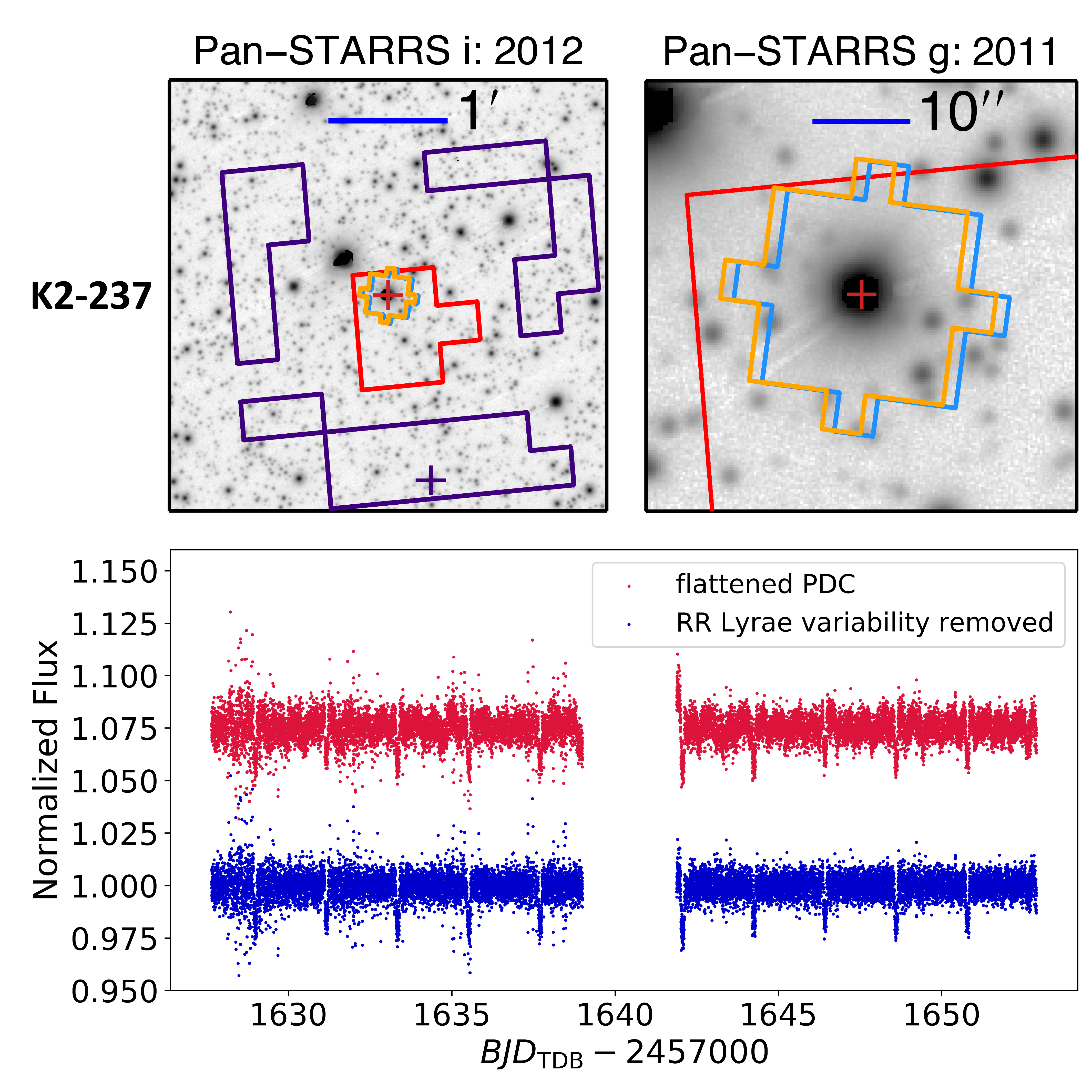
The 5-day rotational modulation signal was not detectable in the TESS lightcurve of K2-237. This may be due to the fact that the TESS and K2 baselines do not temporally overlap and are separated by nearly 900 days. Starspot evolution can lead to changes in observed period and amplitude, and spot constrasts in the redder TESS bandpass can also suppress amplitudes (Oelkers et al. 2018). Instead, the TESS light curve, shown in full in Figure 3, revealed an RR-Lyrae-like signal with a period of days and an amplitude of 4200 ppm. This signal was not seen in the K2 light curve. Given that the TESS pixel scale of 21 arcsec is significantly larger than the K2 pixel scale of 4 arcsec, we attributed the 0.53-day variability signal to one of the nearby contaminating stars, which was confirmed by the SPOC Data Validation (Twicken et al. 2018; Li et al. 2019). Specifically, in addition to detecting the signature of TOI 1049.01 (K2-237 b), a second TCE was generated with a period of 0.529 days in the SPOC Data Validation component. The difference image for this TCE in the SPOC data validation report showed a single pixel at the upper edge of the postage stamp that was highly anti-correlated with the transit signature. There was only one TIC object on that pixel (TIC 16288004). This indicates that the 0.527-day signature was introduced into the light curve through the background correction. Simbad indicates that the star at the coordinates of TIC 16288004 is a known RR Lyr variable, KY Oph (96 from K2-237, see Figure 3). We did not detect any periodic variability in any of the light curves of the other three stars.
II.4 Archival Spectroscopy
For three of the four K2 systems analyzed in this work (all but K2-167), we obtained the archival radial velocity (RV) measurements from the literature (Figure 4). We combined these archival observations with the transit light curves extracted from the photometric observations from K2 and TESS to provide updated system parameters and ephemerides for future follow up efforts. For K2-261 b we used 12 RV observations from the FIbre-fed Échelle Spectrograph (FIES; Telting et al. 2014), 9 RVs from the High Accuracy Radial velocity Planet Searcher for the Northern hemisphere (HARPS-N; Cosentino et al. 2012), and 11 RVs from the High Accuracy Radial velocity Planet Searcher (HARPS; Mayor et al. 2003) that were used in the discovery paper (Johnson et al. 2018). For K2-114, we used the 5 RV observations from the High Resolution Echelle Spectrometer (HIRES, Vogt et al. 1994) on the Keck I telescope (Shporer et al. 2017). With only 5 observations, the global fit has fewer degrees of freedom, and therefore a limited ability to constrain the jitter within the fit. Therefore, we provide a conservative uniform bound on the jitter variance of the fit of 300 on the KECK HIRES RVs for K2-114 b. The discovery of K2-237 b was led by two separate teams (Soto et al. 2018; Smith et al. 2019), with RV observations coming from three separate facilities: FIES (10), HARPS (11), and the CORALIE (9) spectrograph (Queloz et al. 2000). The 11 RV observations from HARPS were treated separately, with 4 observations coming from the Soto et al. 2018 reduction and 7 coming from the reduction done by Smith et al. 2019. These observations were reduced in different manners, so we treated them as separate facilities in our global model (with unique jitter and gamma parameters).
K2-167 b was statistically validated as part of a larger effort for K2 campaigns 0 to 10 (Mayo et al. 2018). There was no mass measured for this system; we did not have any RVs to include in our fit. We also used the determined metallicity from the discovery papers as a prior on our global fit (see Section III). Specifically, we use an [Fe/H] metallicity of 0.4100.037 dex (K2-114, Shporer et al. 2017), 0.450.08 dex (K2-167, Mayo et al. 2018), 0.140.05 dex (K2-237, Soto et al. 2018), and 0.360.06 dex (K2-261, Johnson et al. 2018).
| Parameter | Description (Units) | K2-114 | K2-167 | K2-237 | K2-261⋆ | |
| Probability. | 100 % | 100 % | 100 % | 75.7 % | 24.2 % | |
| Stellar Parameters: | ||||||
| . | Mass (). | |||||
| . | Radius (). | |||||
| . | Luminosity (). | |||||
| . | Density (cgs). | |||||
| . | Surface gravity (cgs). | |||||
| . | Effective Temperature (K). | |||||
| . | Metallicity (dex). | |||||
| . | Initial Metallicity . | |||||
| . | Age (Gyr). | |||||
| . | Equal Evolutionary Phase . | |||||
| . | V-band extinction (mag). | — | — | — | — | |
| . | SED photometry error scaling . | — | — | — | — | |
| Planetary Parameters: | b | |||||
| . | Period (days). | |||||
| . | Radius (). | |||||
| . | Mass (). | — | ||||
| . | Time of conjunction (). | |||||
| . | Optimal conjunction Time (). | |||||
| . | Semi-major axis (AU). | |||||
| . | Inclination (Degrees). | |||||
| . | Eccentricity . | |||||
| . | Argument of Periastron (Degrees). | |||||
| . | Equilibrium temperature (K). | |||||
| . | RV semi-amplitude (m/s). | — | ||||
| . | Log of RV semi-amplitude . | — | ||||
| . | Radius of planet in stellar radii . | |||||
| . | Semi-major axis in stellar radii . | |||||
| . | Transit depth (fraction). | |||||
| . | Ingress/egress transit duration (days). | |||||
| . | Total transit duration (days). | |||||
| . | FWHM transit duration (days). | |||||
| . | Transit Impact parameter . | |||||
| . | Eclipse impact parameter . | |||||
| . | Ingress/egress eclipse duration (days). | |||||
| . | Total eclipse duration (days). | |||||
| . | FWHM eclipse duration (days). | |||||
| . | Blackbody eclipse depth at 3.6m (ppm). | |||||
| . | Blackbody eclipse depth at 4.5m (ppm). | |||||
| . | Density (cgs). | — | ||||
| . | Surface gravity . | — | ||||
| . | Incident Flux (109 erg s-1 cm-2). | |||||
| . | Time of Periastron (). | |||||
| . | Time of eclipse (). | |||||
| . | Time of Ascending Node (). | |||||
| . | Time of Descending Node (). | |||||
| . | . | |||||
| . | . | |||||
| . | Minimum mass (). | — | ||||
| . | Mass ratio . | — | ||||
NOTES:
⋆The global solution for K2-261 b showed a clear bimodality in the host star’s mass and age (see Figure 5 and §III.2). We extract a solution and a probability for each peak, which are both shown in the table. The lower stellar mass (and high age) solution is significantly more likely, but both solutions are presented for future studies on K2-261 b.
See Table 3 in Eastman et al. 2019 for a list of the derived and fitted parameters in EXOFASTv2.
†Minimum covariance with period.
All values in this table for the secondary occultation are predicted values from our global analysis.
See §III for a description of how the EXOFASTv2 fit was conducted and what priors were used for each fit.
| Wavelength Parameters: | Kepler | TESS | |||
|---|---|---|---|---|---|
| K2-114 | |||||
| . | linear limb-darkening coeff . | ||||
| . | quadratic limb-darkening coeff . | ||||
| . | Dilution from neighboring stars . | – | |||
| K2-167 | |||||
| . | linear limb-darkening coeff . | ||||
| . | quadratic limb-darkening coeff . | ||||
| . | Dilution from neighboring stars . | – | |||
| K2-237 | |||||
| . | linear limb-darkening coeff . | ||||
| . | quadratic limb-darkening coeff . | ||||
| . | Dilution from neighboring stars . | ||||
| K2-261 | |||||
| . | linear limb-darkening coeff . | ||||
| . | quadratic limb-darkening coeff . | ||||
| . | Dilution from neighboring stars . | – | |||
| K2-114 | |||||
| Velocity Parameters: | Keck HIRES | ||||
| . | Relative RV Offset (m/s). | ||||
| . | RV Jitter (m/s). | ||||
| . | RV Jitter Variance . | ||||
| Transit Parameters: | K2 C5 (Kepler) | K2 C18 (Kepler) | TESS | ||
| . | Added Variance . | ||||
| . | Baseline flux . | ||||
| K2-167 | |||||
| Transit Parameters: | K2 C3 (Kepler) | TESS | |||
| . | Added Variance . | ||||
| . | Baseline flux . | ||||
| K2-237 | |||||
| Velocity Parameters: | CORALIE | FIES | HARPS (Smith) | HARPS (Soto) | |
| . | Relative RV Offset (m/s). | ||||
| . | RV Jitter (m/s). | ||||
| . | RV Jitter Variance . | ||||
| Transit Parameters: | K2 (Kepler) | K2 (Kepler) | TESS | ||
| . | Added Variance . | ||||
| . | Baseline flux . | ||||
| K2-261 | |||||
| Velocity Parameters: | FIES | HARPS | HARPSN | ||
| . | Relative RV Offset (m/s). | ||||
| . | RV Jitter (m/s). | ||||
| . | RV Jitter Variance . | ||||
| . | Added Variance . | ||||
| . | Baseline flux . | ||||
| Transit Parameters: | K2 (Kepler) | TESS | |||
NOTES:
⋆The global solution for K2-261 b showed a clear bimodality in the host star’s mass and age (see Figure 5 and Section III.2). The transit, velocity, and wavelength parameters shown in this table for K2-261 are for the preferred solution only.
⋆⋆The RV jitter variance for K2-114 b was constrained to 300 .
See Table 3 in Eastman et al. 2019 for a list of the derived and fitted parameters in EXOFASTv2.
All values in this table for the secondary occultation are predicted values from our global analysis.
See §III for a description of how the EXOFASTv2 fit was conducted and what priors were used for each fit.
III EXOFASTv2 Global Fits
The advent of new software packages allows us to more easily combine the archival observations (K2 photometry and RVs) with new data from TESS. Additionally, with the ongoing success of the Gaia mission, we now know the distances to almost every known planet host, allowing us to accurately characterize the host star through a combination of spectral energy distributions, Gaia parallaxes, and updated stellar models. To refine the ephemerides and system parameters of the four K2 systems, we used the exoplanet fitting suite, EXOFASTv2 (Eastman et al. 2013; Eastman 2017; Eastman et al. 2019). In each case other than K2-237 (see Section III.1), we first conducted a preliminary fit of the entire system using EXOFASTv2 to get an estimate for the surface gravity of the host star. We then performed a fit of the spectral energy distribution (SED) of the host star with EXOFASTv2, using the determined stellar surface gravity () as a starting point with a loose 0.25 dex Gaussian prior. We also included Gaussian priors on the stellar metallicity () from the discovery paper (see Section II.4) and parallax from Gaia, and constrained the maximum line of sight extinction (AV) for each system using the galactic dust maps from Schlegel et al. 1998 and Schlafly & Finkbeiner 2011. The precision on fundamental stellar parameters like and the stellar effective temperature () should be limited to the precision of stellar radii measurements from interferometry (White et al. 2018). The SED fit provided values on the stellar effective temperature ( ) and stellar radius () that were too precise, so we used the resulting and with the adopted fractional errors of 1.5% (for ) and 3.5% (for ) as Gaussian priors on the full global fit. This resulted in a prior on and of 0.8100.0284 and 4930.082.0 K for K2-114, 1.6640.058 and 6182.093.0 K for K2-167, and 1.4670.052 and 5449.082.0 K for K2-261. Specifically, for each system we simultaneously fit the TESS (see Section II.2) and K2 (see Section II.1) photometry with the archival RV data (see Section II.4). In the case of K2-167, no radial velocity observations are available (Mayo et al. 2018), so we globally modeled only the photometric data. Within the fit, the mass, radius, and age of the host star are are constrained by the MESA Isochrones and Stellar Tracks (MIST) stellar evolution models (Dotter 2016; Choi et al. 2016; Paxton et al. 2011; Paxton et al. 2013; Paxton et al. 2015). In every case, we allow EXOFASTv2 to fit a dilution term to the TESS light curve, using the the K2 lightcurve as a reference. In all cases, the the dilution term on the TESS light curve is consistent with zero at 2. Since we adjusted the K2 light curve from the standard pipeline (see Section II.1), we allow EXOFASTv2 to fit a dilution term for the K2 lightcurve as well in this fit but bound it with a conservative 5% prior around zero. The dilution term for the K2 lightcurve is consistent with zero at 1. In all cases, we aimed for strict convergence criteria that required a Gelman–Rubin statistic (Gelman & Rubin 1992) of less than 1.01 and at least 1000 independent draws in each parameter. The results are shown in Figures 2 and 4, and Tables 3 and 4.

III.1 K2-237 Global Fit
For the K2-237 system, we ran the full global model slightly differently than as described in the previous section. Specifically, the SED was far less constraining on the fundamental stellar parameters, due to the target lacking Tycho BT and VT magnitudes and the maximum line-of-sight extinction being higher than is typical. Therefore, we included the SED within the global model, placing Gaussian priors on the Gaia parallax and the from Soto et al. 2018 (see Section II.4) and an upper limit on the maximum line of sight extinction (AV) from Schlegel et al. 1998 and Schlafly & Finkbeiner 2011. The resulting parameters have larger uncertainties than for the other systems.
III.2 K2-261 Bimodality
When analyzing the probability distribution function (PDF) for the host star’s mass and age for K2-261, we noticed a bimodality (see Figure 5). The peaks are centered at 1.09 (9.3 Gyr) and 1.27 (4.84 Gyr), with the lower mass solution having a 76.1% probability of being correct from our analysis. With no optimal way to properly represent the PDF due to the bimodality, we split the host star’s mass at the minimum value between the two peaks in the posterior distribution at M⋆ = 1.19 , and extracted two solutions, one for each mass peak. The two solutions are shown in Table 3. There are no significant differences in the systematic parameters resulting from the two solutions; we believe the bimodality is astrophysical. We adopt the solution for M⋆ = 1.09 , but we present both solutions, as they may be important for future studies on K2-261 b.
| Discovery | Updated | |
|---|---|---|
| K2-114 | ||
| P⋆ | (11.391013) d | (11.3909311 0.0000034) d |
| T0 | (2457151.714930.00069) BJD | (2457664.30683) BJD |
| 3 | 2.5 hours | 3 minutes |
| 3 | 5.1 hours | 5 minutes |
| 3 | 7.6 hours | 8 minutes |
| K2-167 | ||
| P | (9.977481) d | (9.9785700.000022) d |
| T0 | (2456979.93678) BJD | (2457349.13970.0018) BJD |
| 3 | 14 hours | 26 minutes |
| 3 | 27.5 hours | 45 minutes |
| 3 | 40.6 hours | 1.1 hours |
| K2-237 | ||
| P⋆⋆ | (2.1805577 0.0000057) d | (2.18053539) d |
| T0 | (2457656.46337890.0000048) BJD | (2457702.255123) BJD |
| 3 | 13 minutes | 2 minutes |
| 3 | 34 minutes | 5 minutes |
| 3 | 55 minutes | 8 minutes |
| K2-261 | ||
| P | (11.63344 0.00012) d | (11.633478 0.000017) d |
| T0 | (2457906.84084) BJD | (2457976.64192) BJD |
| 3 | 45 minutes | 7 minutes |
| 3 | 2.1 hours | 19 minutes |
| 3 | 3.5 hours | 30 minutes |
NOTES:
⋆The new period for K2-114 b is also consistent with the period reported in the earlier discovery paper (Shporer et al. 2017).
⋆⋆The new period for K2-237 b is discrepant with Smith et al. 2019 reported period but consistent with less precise period reported by Soto et al. 2018.
IV Discussion
With the focus of future missions (like JWST) centered on studying the atmospheres of exoplanets through transmission spectroscopy, precise ephemerides and updated parameters will be crucial for scheduling and interpreting these observations. Additionally, some of these facilities will have a fixed lifetime and very high operating costs. Therefore, we want to be as efficient as possible in using these precious resources, allowing us to maximize their scientific productivity. In this paper, we have presented a case study of four known K2 planetary systems that were observed in the first year of NASA’s TESS mission. Our results show that combining the K2 and TESS data sets (along with archival spectroscopy and Gaia parallaxes) can reduce the uncertainty on the time of future transit by up to an order of magnitude compared to the K2 discovery results. The original and updated ephemerides, with their 1-sigma confidence intervals, are found in Table 5. As compared to the discovery ephemerides, we reduced the uncertainty on the planet’s period by roughly a factor of 66 for K2-114 (Livingston et al. 2019), a factor of 44 for K2-167 (Mayo et al. 2018), and a factor of 7 for both K2-237 (Smith et al. 2019) and K2-261 (Johnson et al. 2018). For K2-237, we compare to Smith et al. 2019 with a 4-sigma discrepancy, but our period is consistent with the other discovery ephemeris from Soto et al. 2018. The reason for the discrepancy in the discovery paper results is unclear. Edwards et al. 2020 independently refined the ephemeris of K2-237 using TESS observations and found a period that is consistent to 1 sigma with our result. Our results also provide updated planetary parameters for each system (see Table 3), which will be important for interpreting any future follow up results.
Prior to our analysis, the uncertainties on the periods from the K2 discovery papers propagate to produce high uncertainty (hours to days) on the predicted transit times within the next decade (see Figure 6). The 3-sigma uncertainties on the transit times predicted by the discovery ephemerides, shown in Table 5, are as high as 40.6 hours by 2030 (for K2-167). Because the addition of the TESS data enables such major improvement in precision on the period, the uncertainties on our predicted transit times are dominated by the uncertainty on the time of conjunction, meaning that the total uncertainty on the ephemeris grows much more slowly with time. Our results allow transit times predicted to within 30 minutes with 3-sigma confidence through at least 2030, except for K2-167 b which has a transit uncertainty of 1.1 hours in 2030 (as compared to the 40.6 hour uncertainty the discovery ephemeris would provide, see Table 5 and Figure 6). Therefore, K2-167 b would likely require additional transit follow up over the next few years to have an ephemeris precise enough to enable JWST observations near the expected end of the mission.

V Conclusion
Using observations from the K2 and TESS missions combined with archival spectroscopy, we reanalyzed four known K2 planetary systems, providing updated system parameters and improved ephemerides for future follow up efforts. Additionally, we combined the known parallax for each system from the Gaia mission, allowing us to refine the stellar parameters within our global fits. We performed this case study on K2-114 b, K2-167 b, K2-237 b, and K2-261 b, and our updated ephemerides reduced the uncertainty on the orbital period by factors between 7 and 66. As a result of extending the photometric baseline for each system, we are now able to confidently predict future transit times to within 1 hour through the extent of the JWST prime mission. Additionally, TESS will observe roughly half of all K2 campaigns during the first extended mission, providing the first opportunity to perform an analysis similar to what is presented here, but on a much larger scale (hundreds of systems). This work also shows the importance of updating and maintaining accurate ephemerides, as most known exoplanets have not been reobserved, until recently by TESS. Therefore, it is likely that many of the known planet ephemerides are, or will be, stale, limiting the ability to conduct detailed follow-up. The TESS discovered exoplanet ephemerides will also quickly degrade since most will only be discovered with a 27 day baseline of observations (Dragomir et al. 2020). Continued monitoring and updating of transit ephemerides will likely be necessary to conduct future targeted follow-up observations, and this paper is part of a larger effort to reanalyze previously discovered planets using observations from new missions like Gaia and TESS. Future work should use the method presented here to reanalyze all known exoplanets observed by TESS, providing the community with a larger pool of targets on which to perform detailed characterization in the era of JWST.
References
- Bakos et al. (2010) Bakos, G. Á., Torres, G., Pál, A., et al. 2010, ApJ, 710, 1724
- Barclay & Barentsen (2018) Barclay, T., & Barentsen, G. 2018, Research Notes of the American Astronomical Society, 2, 192
- Benneke et al. (2017) Benneke, B., Werner, M., Petigura, E., et al. 2017, ApJ, 834, 187
- Borucki et al. (2010) Borucki, W. J., Koch, D., Basri, G., et al. 2010, Science, 327, 977
- Bryson et al. (2010) Bryson, S. T., Tenenbaum, P., Jenkins, J. M., et al. 2010, ApJ, 713, L97
- Butters et al. (2010) Butters, O. W., West, R. G., Anderson, D. R., et al. 2010, A&A, 520, L10
- Choi et al. (2016) Choi, J., Dotter, A., Conroy, C., et al. 2016, ApJ, 823, 102
- Collins et al. (2017) Collins, K. A., Kielkopf, J. F., Stassun, K. G., & Hessman, F. V. 2017, AJ, 153, 77
- Cosentino et al. (2012) Cosentino, R., Lovis, C., Pepe, F., et al. 2012, in Proc. SPIE, Vol. 8446, Ground-based and Airborne Instrumentation for Astronomy IV, 84461V
- Cutri et al. (2003) Cutri, R. M., Skrutskie, M. F., van Dyk, S., et al. 2003, VizieR Online Data Catalog, 2246, 0
- Delrez et al. (2018) Delrez, L., Gillon, M., Queloz, D., et al. 2018, in Society of Photo-Optical Instrumentation Engineers (SPIE) Conference Series, Vol. 10700, Proc. SPIE, 107001I
- Dittmann et al. (2017) Dittmann, J. A., Irwin, J. M., Charbonneau, D., Berta-Thompson, Z. K., & Newton, E. R. 2017, AJ, 154, 142
- Dotson et al. (2020) Dotson, J., Colon, K., Barentsen, G., Gully-Santiago, M., & Hedges, C. 2020, in American Astronomical Society Meeting Abstracts, Vol. 52, American Astronomical Society Meeting Abstracts, 174.05
- Dotter (2016) Dotter, A. 2016, ApJS, 222, 8
- Dragomir et al. (2020) Dragomir, D., Harris, M., Pepper, J., et al. 2020, AJ, 159, 219
- Eastman (2017) Eastman, J. 2017, EXOFASTv2: Generalized publication-quality exoplanet modeling code, Astrophysics Source Code Library, ascl:1710.003
- Eastman et al. (2013) Eastman, J., Gaudi, B. S., & Agol, E. 2013, PASP, 125, 83
- Eastman et al. (2019) Eastman, J. D., Rodriguez, J. E., Agol, E., et al. 2019, arXiv e-prints, arXiv:1907.09480
- Edwards et al. (2020) Edwards, B., Changeat, Q., Yip, K. H., et al. 2020, MNRAS, arXiv:2005.01684
- Flewelling et al. (2016) Flewelling, H. A., Magnier, E. A., Chambers, K. C., et al. 2016, arXiv e-prints, arXiv:1612.05243
- Gaia Collaboration et al. (2018) Gaia Collaboration, Brown, A. G. A., Vallenari, A., et al. 2018, A&A, 616, A1
- Gardner et al. (2006) Gardner, J. P., Mather, J. C., Clampin, M., et al. 2006, Space Sci. Rev., 123, 485
- Gaudi et al. (2018) Gaudi, B. S., Seager, S., Mennesson, B., et al. 2018, Nature Astronomy, 2, 600
- Gelman & Rubin (1992) Gelman, A., & Rubin, D. B. 1992, Statistical Science, 7, 457
- Gillon et al. (2011) Gillon, M., Jehin, E., Magain, P., et al. 2011, in European Physical Journal Web of Conferences, Vol. 11, European Physical Journal Web of Conferences, 06002
- Høg et al. (2000) Høg, E., Fabricius, C., Makarov, V. V., et al. 2000, A&A, 355, L27
- Howell et al. (2014) Howell, S. B., Sobeck, C., Haas, M., et al. 2014, PASP, 126, 398
- Huang et al. (2018) Huang, C. X., Burt, J., Vanderburg, A., et al. 2018, ApJ, 868, L39
- Irwin et al. (2015) Irwin, J. M., Berta-Thompson, Z. K., Charbonneau, D., et al. 2015, in Cambridge Workshop on Cool Stars, Stellar Systems, and the Sun, Vol. 18, 18th Cambridge Workshop on Cool Stars, Stellar Systems, and the Sun, ed. G. T. van Belle & H. C. Harris, 767–772
- Jenkins (2002) Jenkins, J. M. 2002, ApJ, 575, 493
- Jenkins et al. (2010) Jenkins, J. M., Caldwell, D. A., Chandrasekaran, H., et al. 2010, ApJ, 713, L120
- Jenkins et al. (2016) Jenkins, J. M., Twicken, J. D., McCauliff, S., et al. 2016, in Proc. SPIE, Vol. 9913, Software and Cyberinfrastructure for Astronomy IV, 99133E
- Johnson et al. (2018) Johnson, M. C., Dai, F., Justesen, A. B., et al. 2018, MNRAS, 481, 596
- Li et al. (2019) Li, J., Tenenbaum, P., Twicken, J. D., et al. 2019, PASP, 131, 024506
- Lightkurve Collaboration et al. (2018) Lightkurve Collaboration, Cardoso, J. V. d. M. a., Hedges, C., et al. 2018, Lightkurve: Kepler and TESS time series analysis in Python, ascl:1812.013
- Livingston et al. (2019) Livingston, J. H., Crossfield, I. J. M., Werner, M. W., et al. 2019, AJ, 157, 102
- Mayo et al. (2018) Mayo, A. W., Vanderburg, A., Latham, D. W., et al. 2018, AJ, 155, 136
- Mayor et al. (2003) Mayor, M., Pepe, F., Queloz, D., et al. 2003, The Messenger, 114, 20
- Oelkers et al. (2018) Oelkers, R. J., Rodriguez, J. E., Stassun, K. G., et al. 2018, AJ, 155, 39
- Paxton et al. (2011) Paxton, B., Bildsten, L., Dotter, A., et al. 2011, ApJS, 192, 3
- Paxton et al. (2013) Paxton, B., Cantiello, M., Arras, P., et al. 2013, ApJS, 208, 4
- Paxton et al. (2015) Paxton, B., Marchant, P., Schwab, J., et al. 2015, ApJS, 220, 15
- Pepper et al. (2012) Pepper, J., Kuhn, R. B., Siverd, R., James, D., & Stassun, K. 2012, PASP, 124, 230
- Pepper et al. (2007) Pepper, J., Pogge, R. W., DePoy, D. L., et al. 2007, PASP, 119, 923
- Queloz et al. (2000) Queloz, D., Mayor, M., Weber, L., et al. 2000, A&A, 354, 99
- Ricker et al. (2015) Ricker, G. R., Winn, J. N., Vanderspek, R., et al. 2015, Journal of Astronomical Telescopes, Instruments, and Systems, 1, 014003
- Roberge & Moustakas (2018) Roberge, A., & Moustakas, L. A. 2018, Nature Astronomy, 2, 605
- Rodriguez et al. (2019) Rodriguez, J. E., Quinn, S. N., Huang, C. X., et al. 2019, AJ, 157, 191
- Savitzky & Golay (1964) Savitzky, A., & Golay, M. J. E. 1964, Analytical Chemistry, 36, 1627
- Schlafly & Finkbeiner (2011) Schlafly, E. F., & Finkbeiner, D. P. 2011, ApJ, 737, 103
- Schlegel et al. (1998) Schlegel, D. J., Finkbeiner, D. P., & Davis, M. 1998, ApJ, 500, 525
- Shporer et al. (2017) Shporer, A., Zhou, G., Fulton, B. J., et al. 2017, AJ, 154, 188
- Smith et al. (2019) Smith, A. M. S., Csizmadia, S., Gandolfi, D., et al. 2019, Acta Astron., 69, 135
- Smith et al. (2012) Smith, J. C., Stumpe, M. C., Van Cleve, J. E., et al. 2012, PASP, 124, 1000
- Soto et al. (2018) Soto, M. G., Díaz, M. R., Jenkins, J. S., et al. 2018, MNRAS, 478, 5356
- Stassun & Torres (2018) Stassun, K. G., & Torres, G. 2018, ApJ, 862, 61
- Stumpe et al. (2014) Stumpe, M. C., Smith, J. C., Catanzarite, J. H., et al. 2014, PASP, 126, 100
- Stumpe et al. (2012) Stumpe, M. C., Smith, J. C., Van Cleve, J. E., et al. 2012, PASP, 124, 985
- Szentgyorgyi et al. (2016) Szentgyorgyi, A., Baldwin, D., Barnes, S., et al. 2016, Society of Photo-Optical Instrumentation Engineers (SPIE) Conference Series, Vol. 9908, The GMT-Consortium Large Earth Finder (G-CLEF): an optical Echelle spectrograph for the Giant Magellan Telescope (GMT), 990822
- Telting et al. (2014) Telting, J. H., Avila, G., Buchhave, L., et al. 2014, Astronomische Nachrichten, 335, 41
- Thompson et al. (2018) Thompson, S. E., Coughlin, J. L., Hoffman, K., et al. 2018, ApJS, 235, 38
- Twicken et al. (2018) Twicken, J. D., Catanzarite, J. H., Clarke, B. D., et al. 2018, PASP, 130, 064502
- Vanderburg & Johnson (2014) Vanderburg, A., & Johnson, J. A. 2014, PASP, 126, 948
- Vanderburg et al. (2015) Vanderburg, A., Montet, B. T., Johnson, J. A., et al. 2015, The Astrophysical Journal, 800, 59
- Vanderburg et al. (2016a) Vanderburg, A., Becker, J. C., Kristiansen, M. H., et al. 2016a, ApJ, 827, L10
- Vanderburg et al. (2016b) Vanderburg, A., Latham, D. W., Buchhave, L. A., et al. 2016b, ApJS, 222, 14
- Vanderspek et al. (2019) Vanderspek, R., Huang, C. X., Vanderburg, A., et al. 2019, ApJ, 871, L24
- Virtanen et al. (2020) Virtanen, P., Gommers, R., Oliphant, T. E., et al. 2020, Nature Methods, 17, 261
- Vogt et al. (1994) Vogt, S. S., Allen, S. L., Bigelow, B. C., et al. 1994, in Proc. SPIE, Vol. 2198, Instrumentation in Astronomy VIII, ed. D. L. Crawford & E. R. Craine, 362
- Wheatley et al. (2018) Wheatley, P. J., West, R. G., Goad, M. R., et al. 2018, MNRAS, 475, 4476
- White et al. (2018) White, T. R., Huber, D., Mann, A. W., et al. 2018, MNRAS, 477, 4403
- Zacharias et al. (2017) Zacharias, N., Finch, C., & Frouard, J. 2017, VizieR Online Data Catalog, 1340