跳到论文正文
W Papers独立论文阅读器 arXiv:2007.00399 论文正文 计算阅读时间 · 0%
引用这篇论文根据当前论文元数据生成,正式投稿前建议核对。


License: arXiv.org perpetual non-exclusive license
arXiv:2007.00399v1 [cs.LG] 01 Jul 2020

Online Robust Regression via SGD on the ℓ1\ell_{1} loss

Scott Pesme Affiliation: EPFL    Nicolas Flammarion Affiliation: EPFL
Abstract

We consider the robust linear regression problem in the online setting where we have access to the data in a streaming manner, one data point after the other. More specifically, for a true parameter θ∗\theta^{*}, we consider the corrupted Gaussian linear model y=⟨x,θ∗⟩+ε+by=\langle x,\ \theta^{*}\rangle+\varepsilon+b where the adversarial noise bb can take any value with probability η\eta and equals zero otherwise. We consider this adversary to be oblivious (i.e., bb independent of the data) since this is the only contamination model under which consistency is possible. Current algorithms rely on having the whole data at hand in order to identify and remove the outliers. In contrast, we show in this work that stochastic gradient descent on the ℓ1\ell_{1} loss converges to the true parameter vector at a O~​(1/(1−η)2​n)\tilde{O}(1/(1-\eta)^{2}n) rate which is independent of the values of the contaminated measurements. Our proof relies on the elegant smoothing of the non-smooth ℓ1\ell_{1} loss by the Gaussian data and a classical non-asymptotic analysis of Polyak-Ruppert averaged SGD. In addition, we provide experimental evidence of the efficiency of this simple and highly scalable algorithm.

1 Introduction

Robust learning is a critical field that seeks to develop efficient algorithms that can recover an underlying model despite possibly malicious corruptions in the data. In recent decades, being able to deal with corrupted measurements has become of crucial importance. The applications are considerable, to name a few settings: computer vision [86, 89, 5], economics [84, 72, 91], astronomy [71], biology [88, 75] and above all, safety-critical systems [14, 39, 32].

Linear regression being one of the most fundamental statistical model, the robust regression problem has naturally drawn substantial attention. In this problem, we wish to recover a signal from noisy linear measurements where an unknown proportion η\eta has been arbitrarily perturbed. Various models have been proposed to illustrate such contaminations. The broadest is to consider that the adversary is adaptive and is allowed to inspect the samples before changing a fraction η\eta. In this general framework, exact model recovery is not possible and several robust algorithms have been proposed [18, 48, 21, 67, 76, 16, 54, 53]. The information-theoretic optimal recovery guarantee has recently been reached by [27]. Another model is to consider an oblivious adversary, in this simpler context it is possible to consistently recover the model parameter and several algorithms have been proposed [8, 78].

However, none of these algorithms are suitable for online or large-scale problems [57, 35]. Indeed, all of the suggested algorithms require handling the complete dataset, which is simply unrealistic in such settings. This is a considerable problem when we know that modern problems involve colossal datasets and that current machine learning methods are limited by the computing time rather than the amount of data [12]. Such considerations advocate the necessity of proposing practical, online and highly scalable robust algorithms, hence we ask the following question:

  • Can we design an efficient online algorithm for the robust regression problem ?

In this paper we answer by the affirmative for the online oblivious response corruption model where we are given a stream of i.i.d. observation (xi,yi)i∈ℕ(x_{i},y_{i})_{i\in\mathbb{N}} from the following generative model:

y=⟨x,θ∗⟩+ε+b,y=\langle x,\ \theta^{*}\rangle+\varepsilon+b,

where θ∗∈ℝd\theta^{*}\in\mathbb{R}^{d} is the true parameter we wish to recover, xx is the Gaussian feature, ε\varepsilon is the Gaussian noise of variance σ2\sigma^{2} and bb is an adversarial ’sparse’ noise supposed independent of the data (x,ε)(x,\varepsilon) such that ℙ⁡(b≠0)=η\mathbb{P}(b\neq 0)=\eta. In order to recover the parameter θ∗\theta^{*}, we perform averaged SGD on the expected ℓ1\ell_{1} loss 𝔼⁡[|y−⟨x,θ⟩|]\mathbb{E}\left[\left|y-\langle x,\ \theta\rangle\right|\right]. Though this algorithm is very simple, we show that it successively handles the outliers in an online manner and consequently recovers the true parameter at the optimal non-asymptotic convergence rate O~​(1/n)\tilde{O}(1/n) for any outlier proportion η<1\eta<1. Such an algorithm is useful for abundant practical applications such as : (a) detection of irrelevant measurements and systematic labelling errors [51], (b) real time detection of system attacks such as frauds by click bots [40] or malware recommendation rating-frauds [94], and (c) online regression with heavy-tailed noise [78].

The minimisation problem minθ∈ℝd⁡𝔼⁡[|y−⟨x,θ⟩|]\min_{\theta\in\mathbb{R}^{d}}\mathbb{E}\left[\left|y-\langle x,\ \theta\rangle\right|\right] is certainly not new and is also known as the Least Absolute Deviations (LAD) problem. While originally suggested by Boscovich in the mid-eighteenth century [10], it first appears in the work of Edgeworth [31]. In contrast with least-squares, there is no closed form solution to the problem and, in addition, the non-differentiability of the ℓ1\ell_{1} loss prevents the use of fast optimisation solvers for large-scale applications [87]. However, if successively dealt with, the LAD problem has many advantages. Indeed, the ℓ1\ell_{1} loss is well known for its robustness properties [47] and, unlike the Huber loss [45], it is parameter free which makes it more convenient in practice. In this context, using the SGD algorithm in order to solve the LAD problem is a very natural approach. We show in our analysis that, though the ℓ1\ell_{1} loss is not strongly convex, averaged SGD recovers a remarkable O⁡(1/n)O(1/n) convergence rate instead of the classical O⁡(1/n)O(1/\sqrt{n}) which is ordinary in the non-strongly-convex framework

With a convergence rate depending on the variance as O⁡(σ2​d/(1−η~)2​n)O(\sigma^{2}d/(1-\tilde{\eta})^{2}n), the proposed algorithm has several major benefits: a) it is highly scalable and statistically optimal, b) it depends on the outlier contamination through an effective outlier proportion η~\tilde{\eta} strictly smaller than η\eta, which makes it adaptive to the difficulty of the adversary, c) it is relatively insensitive to the ill conditioning of the features and d) it is almost parameter free since it only requires in practice an upper-bound on the covariates’ norm. Though the algorithm is simple, its analysis is not and requires several technical manipulations based on recent advances in stochastic approximation [43]. Indeed, in the classical non-strongly-convex framework which we are in, the usual convergence rate is O⁡(1/n)O(1/\sqrt{n}) and not O⁡(1/n)O(1/n) as we obtain. Overall our analysis relies on the smoothing of the ℓ1\ell_{1} loss by the Gaussian data. This smoothing enables the retrieval of a fast O⁡(1/n)O(1/n) rate thanks to the local strong convexity around θ∗\theta^{*} and to Polyak-Ruppert averaging.

Our paper is organised as follows. We define the problem which we consider in section 2. We then describe the particular structure our function f⁡(θ):=𝔼⁡[|y−⟨x,θ⟩|]f(\theta):=\mathbb{E}[|y-\langle x,\ \theta\rangle|] enjoys in section 3. Our main convergence guarantee result is given section 4 followed by the sketch of proof in section 5. Finally, in section 6, we provide experimental validation of the performances of our method.

1.1 Related work

Robust statistics.

Classical robust statistics have a long history which begins with the seminal work by Tukey and Huber [81, 45]. They mostly focus on the influence function [42], the asymptotic efficiency [90] as well as on the concept of breakdown point [41, 28] which is the maximal proportion of outliers an estimate can tolerate before it breaks down. However these approaches are purely statistical and the proposed estimators are unfortunately either not computable in polynomial time  [69, 70] or purely heuristical [33].

Recent advances in robust statistics.

[22, 50] are the first to propose robust estimators of the mean that can be computed in polynomial time and that have near optimal sample complexities. This leads to a recent line of work in the computer science community that provides recovery guarantees for a range of different statistical problems such as mean estimation or covariance estimation [23, 26, 24, 49, 44, 76, 16]. The robust linear regression problem is explored under general corruption models in the works of [18, 48, 21, 27, 67, 76, 16, 54, 53]. The broadest and therefore hardest contamination model considers that the adversary has access to all the samples and can arbitrarily contaminate any fraction η\eta. In this contamination framework the minimax optimal estimation rate on ‖θ^−θ∗‖\|\hat{\theta}-\theta^{*}\| is O~​(σ​(η+d/n))\tilde{O}(\sigma(\eta+\sqrt{d/n})) where σ2\sigma^{2} is the variance of the Gaussian dense noise [17]. In [27] this minimax bound is achieved under the assumption that the covariates follow a centered Gaussian distribution of covariance identity. For a general covariance matrix HH, the sample complexity becomes O⁡(d2/η2)O(d^{2}/\eta^{2}), however they provide a statistical query lower bound showing that it may be computationally hard to approximate θ∗\theta^{*} with less than d2d^{2} samples. We highlight the fact that if the computational issues are put aside, [38] provides for the weaker Huber ε\varepsilon contamination model11 1 This contamination model is weaker because the adversary is oblivious of the uncorrupted samples a statistically optimal estimator which can however only be computed in exponential time. For more details on the current advances, see the recent survey [25].

Response corrupted robust regression.

A simpler contamination model is to consider that the adversary can only corrupt the responses and not the features. In this framework two main approaches have been considered.
a) The first approach is based on viewing the regression problem as minθ,b:‖b‖0≤η​n∥y−Xθ−b∥2\min_{\theta,b:\|b\|_{0}\leq\eta n}\|y-X\theta-b\|_{2}. However this is a non-convex and NP hard problem [77]. In order to deal with the problem, convex relaxations based on the ℓ1\ell_{1} loss [85, 63, 62] and second-order-conic-programming (SOCP) [13, 19] have been proposed and studied. Simultaneously, hard thresholding techniques were considered [9, 8, 78]. However all of these approaches rely on manipulating the whole corruption vector b{b} and are therefore not easy to adapt to the online setting.
b) The second approach relies on using a so-called robust loss. This is designated as the M-estimation framework [45]: the least-squares problem is replaced by minθ⁡𝔼z​[ρ⁡(θ,z)]\min_{\theta}\mathbb{E}_{z}[\rho(\theta,z)] where the loss function ρ\rho is chosen for its robustness properties. The ℓ1\ell_{1} loss or the Huber loss [45] are classical examples of convex robust losses. The Huber loss is essentially an appropriate mix of the ℓ2\ell_{2} and the ℓ1\ell_{1} losses. On the other hand the Tukey biweight [81] is an example of a non-convex robust loss. The idea behind such losses is to give less weight to the outliers which have large residuals. Asymptotic normality of these M-estimators have been well studied in the statistical literature [46, 6, 56, 64, 83, 82, 79] and their non-asymptotic performance have been recently investigated [55, 93, 58, 47].

We point out that the two mentioned approaches are related since they are duals. Minimising the Huber Loss is equivalent to the ℓ1\ell_{1} constrained problem minθ,b⁡‖y−X​θ−b‖22+λ​‖b‖1\min_{\theta,b}\|y-X\theta-b\|^{2}_{2}+\lambda\|b\|_{1} for an appropriate λ\lambda [36, 29]. The estimation rates of ‖θ^−θ∗‖2\|\hat{\theta}-\theta^{*}\|_{2} in both cases are similar and typically O~​(σ​(η+d/n))\tilde{O}(\sigma(\sqrt{\eta}+\sqrt{d/n})). These rates were later improved to the optimal rate O~​(σ​(η+d/n))\tilde{O}(\sigma(\eta+\sqrt{d/n})) in [20]. When the adversary is in addition oblivious, consistency is possible and [79, 8, 78] show that there exists a consistent estimator with error O⁡(σ​(1−η)−1​d/n)O(\sigma(1-\eta)^{-1}\sqrt{d/n}).

Stochastic optimisation.

Stochastic optimisation has been studied in a variety of different frameworks such as that of machine learning [11, 92], optimisation [59] and stochastic approximation [7]. The optimal convergence rates are known since [60]: it is of O⁡(1/n)O(1/\sqrt{n}) in the general convex case and is improved to O⁡(1/μ​n)O(1/\mu n) if μ\mu-strong convexity is additionally assumed. These rates are obtained using the SGD algorithm. However the optimal step-size sequences depend on ff’s convexity properties. The idea of averaging the SGD iterates first appears in the works of [65] and [73]. This method is now referred to as Polyak-Ruppert averaging. Shortly after, [66] provides asymptotic normality results on the probability distribution of the averaged iterates. This result is later generalised in [3] where non-asymptotic guarantees are provided. In the smooth framework, the advantages of averaging are numerous. Indeed, it improves the global convergence rate and leads to the statistically optimal asymptotic variance rate which is independent of the conditioning μ\mu [4]. Moreover it has the significant advantage of providing an algorithm that adapts to the difficulty of the problem: with averaging, the same step-size sequence leads to the optimal convergence rate whether the function is strongly convex or not. Averaging also displays another important property which will prove to be particularly relevant in our work: it leads to fast convergence rates in some cases where the function is only locally strongly convex around the solution, as for logistic regression [2].

2 Problem formulation

Consider we have a stream of independent and identically distributed data points (xi,yi)i∈ℕ(x_{i},y_{i})_{i\in\mathbb{N}} sampled from the following linear model:

yi=⟨xi,θ∗⟩+εi+bi,y_{i}=\langle x_{i},\ \theta^{*}\rangle+\varepsilon_{i}+b_{i}, (A.1)

where θ∗∈ℝd\theta^{*}\in\mathbb{R}^{d} is a parameter we wish to recover. The noises εi\varepsilon_{i} are considered as ’nice’ noise of finite variance σ2\sigma^{2}. In contrast the outliers bib_{i} can be any adversarial ’sparse’ noise. In the online setting we define a sparse random variable as a random variable that equals 00 with probability (1−η)∈(0,1](1-\eta)\in(0,1].

We investigate in this work the ℓ1\ell_{1} minimisation problem (a.k.a least absolute deviation):

minθ∈ℝd⁡f⁡(θ):=𝔼⁡[|y−⟨x,θ⟩|],\min_{\theta\in\mathbb{R}^{d}}f(\theta):=\mathbb{E}\left[|y-\langle x,\ \theta\rangle|\right], (1)

using the stochastic gradient descent algorithm [68] defined by the following recursion initialised at θ0∈ℝd\theta_{0}\in\mathbb{R}^{d}:

θn=θn−1+γn​sgn​(yn−⟨xn,θn−1⟩)​xn,\displaystyle\theta_{n}=\theta_{n-1}+\gamma_{n}\text{sgn}\left(y_{n}-\langle x_{n},\ \theta_{n-1}\rangle\right)x_{n}, (2)

where (γn)n≥1(\gamma_{n})_{n\geq 1} is a positive sequence named step-size sequence. In this paper we mostly consider the averaged iterate θ¯n=1n​∑i=0n−1θi\bar{\theta}_{n}=\frac{1}{n}\sum_{i=0}^{n-1}\theta_{i} which can easily be computed online as θ¯n=1n​θn−1+n−1n​θ¯n−1\bar{\theta}_{n}=\frac{1}{n}\theta_{n-1}+\frac{n-1}{n}\bar{\theta}_{n-1}. Note that SGD is an extremely simple and highly scalable streaming algorithm. There are no parameters to tune, we will see further that a step-size sequence of the type γn=1/R2​n\gamma_{n}=1/R^{2}\sqrt{n} leads to a good convergence rate.

We make here the following assumptions:

  1. (A.2)

    Gaussian features. The features xx are centered Gaussian ∼𝒩⁡(0,H)\sim\mathcal{N}(0,H) where HH is a positive definite matrix. We denote by μ\mu its smallest eigenvalue and R2=trace​(H)R^{2}=\text{trace}(H).

  2. (A.3)

    Independent Gaussian dense noise. The dense noise ε\varepsilon is a centered Gaussian 𝒩⁡(0,σ2)\mathcal{N}(0,\sigma^{2}) where σ>0\sigma>0 and ε\varepsilon is independent of xx.

  3. (A.4)

    Independent sparse adversarial noise. The adversarial noise bb is independent of (x,ε)(x,\varepsilon) and satisfies ℙ⁡(b≠0)=η∈[0,1)\mathbb{P}\left(b\neq 0\right)=\eta\in[0,1). We denote by η~=η⋅(1−𝔼b​[exp⁡(−b22​σ2)])∈[0,η)\tilde{\eta}=\eta\cdot\big(1-\mathbb{E}_{b}\big[\operatorname{exp}\big(-\frac{b^{2}}{2\sigma^{2}}\big)\big]\big)\in[0,\eta).

Under these assumptions f′​(θ∗)=−𝔼⁡[sgn​(ε+b)​x]=−𝔼⁡[sgn​(ε+b)]​𝔼​[x]=0f^{\prime}(\theta^{*})=-\mathbb{E}\left[\text{sgn}\left(\varepsilon+b\right)x\right]=-\mathbb{E}\left[\text{sgn}\left(\varepsilon+b\right)\right]\mathbb{E}\left[x\right]=0. It therefore makes sense to minimise ff in order to recover the parameter θ∗\theta^{*}. Note that contrary to least-squares where a finite mean and variance are required, we do not make any assumptions on the moments of the noise bb. The Gaussian assumptions on data are technical and made for simplicity. However the continuous aspect of the features and the noise is essential in order to have a differentiable loss ff after taking the expectation. We point that the Gaussian assumptions is a classical assumption which is also made in the works of [9, 8, 78, 47, 27]. However we do not make any additional hypothesis on matrix HH concerning its conditioning. We point out that in our framework we must have ε\varepsilon and the adversarial noise bb independent of xx in order to have argminθ∈ℝd​𝔼​[|y−⟨x,θ⟩|]=θ∗\text{argmin}_{\theta\in\mathbb{R}^{d}}\ \mathbb{E}\left[\left|y-\langle x,\ \theta\rangle\right|\right]=\theta^{*}. The parameter η~∈[0,η)\tilde{\eta}\in[0,\eta) we introduce in Assumption A.4 is the effective outlier proportion. This quantity expresses the pertinent corruption proportion and will prove to be more relevant than η\eta. Indeed, notice that in the simple case where ℙ⁡(b≪σ)∼1\mathbb{P}\left(b\ll\sigma\right)\sim 1 then 𝔼b[exp(−b2/σ2)]∼1\mathbb{E}_{b}[\operatorname{exp}\left(-{b^{2}}/{\sigma^{2}}\right)]\sim 1 and η~∼0\tilde{\eta}\sim 0. Intuitively in this situation it makes sense to have an effective outlier corruption close to zero: if b≪σb\ll\sigma a.s., then the bib_{i}’s do not disturb the recursion and can therefore be considered as non-adversarial noises. This last observation is however only valid in the oblivious framework.

3 Gaussian smoothing and structure of the objective function ff

In this section we show that ff and its derivatives enjoy nice properties and have closed forms which prove to be useful in analysing the SGD recursion section 5. We fist show that though the ℓ1\ell_{1} loss is not smooth, it turns out that by averaging over the continuous Gaussian features xx and noise ε\varepsilon, the expected loss ff is continuously derivable.

Lemma 1.

Suppose that (A.1, A.2, A.3, A.4) hold and let erf⁡(⋅)\operatorname{erf}\left(\cdot\right) denote the Gauss error function. Then for all θ∈ℝd\theta\in\mathbb{R}^{d}:

f⁡(θ)=𝔼b​[2π​σ2+‖θ−θ∗‖H2​exp⁡(−b22​(σ2+‖θ−θ∗‖H2))+b​erf⁡(b2​(σ2+‖θ−θ∗‖H2))].\displaystyle\textstyle f(\theta)=\mathbb{E}_{b}\left[\sqrt{\frac{2}{\pi}}\sqrt{\sigma^{2}+\left\lVert\theta-\theta^{*}\right\rVert_{H}^{2}}\operatorname{exp}\left(-\frac{b^{2}}{2(\sigma^{2}+\left\lVert\theta-\theta^{*}\right\rVert_{H}^{2})}\right)+b\operatorname{erf}\left(\frac{b}{\sqrt{2(\sigma^{2}+\left\lVert\theta-\theta^{*}\right\rVert_{H}^{2})}}\right)\right].

We point out that the expectation 𝔼b​[⋅]\mathbb{E}_{b}\left[\cdot\right] is taken only over the outlier distribution, the expectation over the Gaussian features and Gaussian noise having already been taken. The proof relies on noticing that since bb is independent of xx and ε\varepsilon, given outlier bb, y−⟨x,θ⟩=ε+b−⟨x,θ−θ∗⟩y-\langle x,\ \theta\rangle=\varepsilon+b-\langle x,\ \theta-\theta^{*}\rangle follows a normal distribution 𝒩⁡(b,σ2+‖θ−θ∗‖H2)\mathcal{N}(b,\sigma^{2}+\left\lVert\theta-\theta^{*}\right\rVert_{H}^{2}). The absolute value of this Gaussian random variable follows a folded normal distribution whose expectation has a closed form [52]. lemma 1 exhibits the fact that though the ℓ1\ell_{1} loss is not differentiable at zero, taking its expectation over a continuous density makes the expected loss ff continuously differentiable. This is reminiscent of Gaussian smoothing used in gradient-free and non-smooth optimisation [61, 30].

In the absence of contamination, i.e., when b=0b=0 almost surely, the function simplifies to the pseudo-Huber loss function [15] with parameter σ\sigma, f⁡(θ)=2/π​(σ2+‖θ−θ∗‖H2)1/2f(\theta)=\sqrt{2/\pi}(\sigma^{2}+\left\lVert\theta-\theta^{*}\right\rVert_{H}^{2})^{1/2}. More broadly, notice that f⁡(θ)∼2/π​‖θ−θ∗‖Hf(\theta){\sim}\sqrt{{2}/{\pi}}\left\lVert\theta-\theta^{*}\right\rVert_{H} when ‖θ−θ∗‖H→+∞\left\lVert\theta-\theta^{*}\right\rVert_{H}\to+\infty and f⁡(θ)−f⁡(θ∗)∼1−η~2​π​σ​‖θ−θ∗‖H2f(\theta)-f(\theta^{*}){\sim}\frac{1-\tilde{\eta}}{\sqrt{2\pi}\sigma}\left\lVert\theta-\theta^{*}\right\rVert_{H}^{2} for ‖θ−θ∗‖H≪σ\left\lVert\theta-\theta^{*}\right\rVert_{H}\ll\sigma. This highlights the quadratic behaviour of ff around the solution θ∗\theta^{*} and its linear behaviour far from it. This shows that though ff is not strongly convex on ℝd\mathbb{R}^{d}, it is locally strongly convex around θ∗\theta^{*}. Actually the two criteria f⁡(θ)−f⁡(θ∗)f(\theta)-f(\theta^{*}) and ‖θ−θ∗‖H\left\lVert\theta-\theta^{*}\right\rVert_{H} are closely related and we show that the prediction error ‖θ−θ∗‖H2\left\lVert\theta-\theta^{*}\right\rVert_{H}^{2} is in fact O⁡(f⁡(θ)−f⁡(θ∗)+(f⁡(θ)−f⁡(θ∗))2)O\left(f(\theta)-f(\theta^{*})+(f(\theta)-f(\theta^{*}))^{2}\right) (see lemma 12 in Appendix).

The next lemma exhibits the fact that f′f^{\prime} has a surprisingly neat structure.

Lemma 2.

Suppose that (A.1, A.2, A.3, A.4) hold. Then for every θ∈ℝd\theta\in\mathbb{R}^{d}:

f′​(θ)=α⁡(‖θ−θ∗‖H)​H​(θ−θ∗),\displaystyle f^{\prime}(\theta)=\alpha(\left\lVert\theta-\theta^{*}\right\rVert_{H})\ H(\theta-\theta^{*}),

with α⁡(z)=2π​1σ2+z2​𝔼b​[exp⁡(−b22​(σ2+z2))]\textstyle\alpha(z)=\sqrt{\frac{2}{\pi}}\frac{1}{\sqrt{\sigma^{2}+z^{2}}}\mathbb{E}_{b}\left[\operatorname{exp}\left(-\frac{b^{2}}{2(\sigma^{2}+z^{2})}\right)\right] for z∈ℝz\in\mathbb{R}.

This result is immediately obtained by deriving ff’s closed form. The gradient f′f^{\prime} benefits from a very specific structure: it is exactly the gradient of the ℓ2\ell_{2} loss with a scalar factor in front which depends on σ\sigma, the outlier distribution and the prediction loss ‖θ−θ∗‖H\left\lVert\theta-\theta^{*}\right\rVert_{H}. Note that the gradient is proportional to HH, this proves to be useful in our analysis. Also note that the gradients are uniformly bounded over ℝd\mathbb{R}^{d} since ‖f′​(θ)‖22≤R2\left\lVert f^{\prime}(\theta)\right\rVert_{2}^{2}\leq R^{2}. This fact, already predictable from the expression of the stochastic gradients, stands in sharp contrast with the ℓ2\ell_{2} loss and illustrates the ℓ1\ell_{1} loss’s robustness property.

Finally the following lemma highlights ff’s local strong convexity around θ∗\theta^{*} which is essential to obtain the O⁡(1/n)O(1/n) convergence rate.

Lemma 3.

Suppose that (A.1, A.2, A.3, A.4) hold. Then

f′′​(θ∗)=2π​1−η~σ​H.f^{\prime\prime}(\theta^{*})=\sqrt{\frac{2}{\pi}}\frac{1-\tilde{\eta}}{\sigma}\ H.

Lemma 3 shows that ff is locally strongly convex around θ∗\theta^{*} with local strong convexity constant 2/π​(1−η~)​μσ\sqrt{{2}{/\pi}}\frac{(1-\tilde{\eta})\mu}{\sigma}. We hence see the impact the effective outlier proportion η~\tilde{\eta} has: the closer it is to one and the worse the local conditioning is. Also note that if there were no additional noise ε\varepsilon, which corresponds to σ→0\sigma\to 0, then there is no smoothing of the ℓ1\ell_{1} loss anymore and the problem becomes non-smooth.

4 Convergence guarantee

The nice properties the function ff enjoys enables a clean analysis of the SGD recursion with decreasing step sizes. The convergence rate we obtain on the averaged iterate θ¯n=1n​∑i=0n−1θi\bar{\theta}_{n}=\frac{1}{n}\sum_{i=0}^{n-1}\theta_{i} is given in the following theorem.

Theorem 4.

Let (A.1, A.2, A.3, A.4) hold and consider the SGD iterates following Eq. (2). Assume γn=γ0n\gamma_{n}=\frac{\gamma_{0}}{\sqrt{n}}. Then for all n≥1n\geq 1:

𝔼⁡[‖θ¯n−θ∗‖H2]\displaystyle\mathbb{E}\left[\left\lVert\bar{\theta}_{n}-\theta^{*}\right\rVert^{2}_{H}\right] =O⁡(σ2​d(1−η~)2​n)+O~​(‖θ0−θ∗‖4γ02​(1−η~)2​n)+O~​(γ02​R4(1−η~)2​n)\displaystyle=O\Big(\frac{\sigma^{2}d}{(1-\tilde{\eta})^{2}n}\Big)+\tilde{O}\Big(\frac{\left\lVert\theta_{0}-\theta^{*}\right\rVert^{4}}{\gamma_{0}^{2}(1-\tilde{\eta})^{2}n}\Big)+\tilde{O}\Big(\frac{\gamma_{0}^{2}R^{4}}{(1-\tilde{\eta})^{2}n}\Big)
+O~​(σ2γ02​μ2​(1−η~)3​n3/2​(‖θ0−θ∗‖2γ0+γ0​R2)).\displaystyle\qquad+\tilde{O}\Big(\frac{\sigma^{2}}{\gamma_{0}^{2}\mu^{2}(1-\tilde{\eta})^{3}n^{3/2}}\Big(\frac{\left\lVert\theta_{0}-\theta^{*}\right\rVert^{2}}{\gamma_{0}}+\gamma_{0}R^{2}\Big)\Big).

For clarity the exact constants are not given here but can be found in the Appendix. Note that the result is given in terms of the Mahalanobis distance associated with the covariance matrix HH which corresponds to the classical prediction error. The overall bound has a dependency in the number of iterations of O⁡(1/n)O(1/n), this is optimal for stochastic approximation even with strong-convexity [60]. We also point out that by a purely naive analysis that does not exploit the specificities of our problem we could easily obtain a O⁡(1/n)O(1/\sqrt{n}) rate, which is the common rate for non-strongly-convex functions.

Notice that the convergence rate is not influenced by the magnitude of the outliers but only by their effective proportion η~∈[0,η)\tilde{\eta}\in[0,\eta) which is, as we could anticipate, more relevant than η\eta. This effective outlier proportion can be considerably smaller than η\eta if a portion of the outliers behave correctly. Therefore the algorithm adapts to the difficulty of the adversary. We also point out that we recover the same dependency in the proportion of outliers as in [79, 8, 78] but with η~\tilde{\eta} in our case, which is strictly better. The question of the optimality of the 1/(1−η~)21/(1-\tilde{\eta})^{2} constant is unknown and is an interesting open problem, a trivial lower bound being 1/(1−η~)1/(1-\tilde{\eta}). Furthermore, in the finite horizon framework where we have NN samples, the breakdown point we obtain is η~=1−Ω⁡(ln3/2⁡NN)\tilde{\eta}=1-\Omega(\frac{\ln^{3/2}N}{\sqrt{N}}). This is better than what is obtain in [78] ( 1−Ω⁡(1ln⁡N)1-\Omega(\frac{1}{\ln N}) ) and the same (to a ln\ln factor) as the asymptotic result from [79].

We now take a closer look at each term. The first term is the dominant variance term and is of the form σ2​dn\frac{\sigma^{2}d}{n}. It is statistically optimal in terms of dd and nn since it is also optimal in the simpler framework where there are no outliers [80]. The second term is the dominant bias term which only depends on the distance between the initial point θ0\theta_{0} and the solution θ∗\theta^{*}. Notice that it is proportional to ‖θ0−θ∗‖4\|\theta_{0}-\theta^{*}\|^{4} as in [2], however we believe the dependency in ‖θ0−θ∗‖\|\theta_{0}-\theta^{*}\| could be improved to O⁡(‖θ0−θ∗‖2)O(\|\theta_{0}-\theta^{*}\|^{2}) by further exploiting the local strong-convexity property. The third term is a by-product of our analysis and comes from the bound on the norm of the stochastic gradients. We conjecture that it could be possible to get rid of it. We highlight that the three dominant O⁡(1/n)O(1/n) terms are independent of the data conditioning constant μ\mu. Finally, the two last terms are higher order terms that depend on μ\mu, they are correcting terms as in [3] due to the fact that our function is not quadratic. Note that all three dominant O⁡(1/n)O(1/n) terms are independent of μ\mu, this is obtained thanks to ff’s structure and is due to the fact that f′f^{\prime} is proportional to HH around θ∗\theta^{*}, as in the least-squares framework. We clearly see the benefits of this result in the experiments section 6: unlike the algorithms from [8, 78] which solve successive least-squares problems and are therefore very sensitive to HH’s conditioning, our algorithm is way less impacted by the ill conditioning.

We underline the fact that the algorithm is parameter free: neither the knowledge of σ\sigma nor of the outlier proportion η\eta are required. Also, note that there is no restriction on the value of γ0\gamma_{0} but in practice setting it to O⁡(1/R2)O(1/R^{2}) leads to the best results. We believe that instead of considering the ℓ1\ell_{1} loss we could have considered the Huber loss and followed the same technical analysis to obtain a O⁡(1/n)O(1/n) rate. However as shown in the experiments section 6, considering the Huber loss does not improve the rate and requires an extra parameter that must be tuned.

5 Sketch of proof

We provide an overview of the arguments that constitute the proof of Theorem 4, the full details can be found in the Appendix. We bring out three key steps. First, using the structure of our problem we relate the behaviour of the averaged iterate θ¯n\bar{\theta}_{n} to the average of the gradient f¯′​(θn)=1n​∑i=0n−1f′​(θi)\bar{f}^{\prime}(\theta_{n})=\frac{1}{n}\sum_{i=0}^{n-1}f^{\prime}(\theta_{i}) (see Lemma 14). Then we show that f¯′​(θn)\bar{f}^{\prime}(\theta_{n}) converges to 00 at the rate O⁡(1/n)O(1/n) (see Lemma 6). Finally we control the additional terms using generic results that hold for non-strongly-convex and non-smooth functions (see Lemma 7). Technical difficulties arise from (a) the fact that we consider a decreasing step-size sequence, which is necessary in order to have a fully online algorithm and (b) the fact that we want to obtain a leading order term O⁡(1/n)O(1/n) independent of the conditioning constant μ\mu.

First we use ff’s specific structure to bound the distance between θ¯n\bar{\theta}_{n} and the solution θ∗\theta^{*}.

Lemma 5.

Let (A.1, A.2, A.3, A.4) hold. Then for any sequences (θi)i=0n−1∈ℝd​n(\theta_{i})^{n-1}_{i=0}\in\mathbb{R}^{dn} their average θ¯n=1n​∑i=0n−1θi\bar{\theta}_{n}=\frac{1}{n}\sum_{i=0}^{n-1}\theta_{i} satisfies:

𝔼⁡[‖θ¯n−θ∗‖H2]≤2​σ2(1−η~)2​𝔼​[‖1n​∑i=0n−1f′​(θi)‖H−12]+800(1−η~)2​(ln⁡21−η)2​𝔼​[(1n​∑k=0n−1⟨f′​(θi),θi−θ∗⟩)2].\displaystyle\textstyle\mathbb{E}\left[\left\lVert\bar{\theta}_{n}-\theta^{*}\right\rVert^{2}_{H}\right]\leq\frac{2\sigma^{2}}{(1-\tilde{\eta})^{2}}\mathbb{E}\left[\left\lVert\frac{1}{n}\sum_{i=0}^{n-1}f^{\prime}(\theta_{i})\right\rVert_{H^{-1}}^{2}\right]+\frac{800}{(1-\tilde{\eta})^{2}}\left(\ln\frac{2}{1-\eta}\right)^{2}\mathbb{E}\left[\left(\frac{1}{n}\sum_{k=0}^{n-1}\langle f^{\prime}(\theta_{i}),\ \theta_{i}-\theta^{*}\rangle\right)^{2}\right].

This result follows from the inequality ‖f′​(θ)−f′′​(θ∗)​(θ−θ∗)‖H−1≤20σ1​(ln⁡21−η)​⟨f′​(θ),θ−θ∗⟩\|f^{\prime}(\theta)-f^{\prime\prime}(\theta^{*})(\theta-\theta^{*})\|_{H^{-1}}\leq\frac{20}{\sigma_{1}}(\ln\frac{2}{1-\eta})\langle f^{\prime}(\theta),\ \theta-\theta^{*}\rangle (see proof in Appendix) which upper-bounds the remainder of the first-order Taylor expansion of the gradient by ff’s linear approximation ⟨f′​(θ),θ−θ∗⟩\langle f^{\prime}(\theta),\ \theta-\theta^{*}\rangle. This inequality is crucial in our analysis since in the non-strongly-convex framework, the averaged linear approximations always converge to zero while the iterates θi\theta_{i} a priori do not converge to θ∗\theta^{*}. This inequality is highly inspired by the self-concordance property of the logistic loss used in [2] but is simpler in our setting thanks to an ad hoc analysis. Note that the result from lemma 14 is valid for any sequence (θi)i≥0(\theta_{i})_{i\geq 0} and not only the one issued from the SGD recursion. The two quantities that we therefore need to control are clear. The first one is central as it leads to the final dominant variance term, the second one is technical and less important, it is left for the end of the section. We first show that ‖f¯′​(θn)‖2\left\lVert\bar{f}^{\prime}(\theta_{n})\right\rVert^{2}, the square norm of the average of the gradients, converges at rate O⁡(1/n)O(1/n).

Lemma 6.

Let (A.1, A.2, A.3, A.4) and consider the SGD iterates following Eq. (2). Assume γn=γ0n\gamma_{n}=\frac{\gamma_{0}}{\sqrt{n}}. Then for all n≥1n\geq 1 :

𝔼⁡[‖1n​∑i=0n−1f′​(θi)‖H−12]≤16​dn\displaystyle\mathbb{E}\left[\left\lVert\frac{1}{n}\sum_{i=0}^{n-1}f^{\prime}(\theta_{i})\right\rVert^{2}_{H^{-1}}\right]\leq\frac{16d}{n} +4n​γ02​𝔼​[‖θn−θ∗‖H−12]+4n2​γ02​‖θ0−θ∗‖H−12\displaystyle+\frac{4}{n\gamma_{0}^{2}}\mathbb{E}\left[\left\lVert\theta_{n}-\theta^{*}\right\rVert_{H^{-1}}^{2}\right]+\frac{4}{n^{2}\gamma_{0}^{2}}\left\lVert\theta_{0}-\theta^{*}\right\rVert_{H^{-1}}^{2}
+4n2​(∑i=1n−1𝔼​[‖θi−θ∗‖H−12]1/2​(1γi+1−1γi))2.\displaystyle+\frac{4}{n^{2}}\Big(\sum_{i=1}^{n-1}\mathbb{E}\left[\left\lVert\theta_{i}-\theta^{*}\right\rVert_{H^{-1}}^{2}\right]^{1/2}\left(\frac{1}{\gamma_{i+1}}-\frac{1}{\gamma_{i}}\right)\Big)^{2}.

The proof technique of the inequality is similar to those of [66, 3, 34] and relies on the classical expansion ∑i=1nfi′​(θi−1)=∑i=1nθi−1−θiγi\sum_{i=1}^{n}f^{\prime}_{i}(\theta_{i-1})=\sum_{i=1}^{n}\tfrac{\theta_{i-1}-\theta_{i}}{\gamma_{i}}. We stress out the fact that from here, one could simply choose to upper bound 𝔼⁡[‖θi−θ∗‖H−12]\mathbb{E}[\left\lVert\theta_{i}-\theta^{*}\right\rVert_{H^{-1}}^{2}] using classical non-strongly convex bounds which would lead to 𝔼⁡[‖θi−θ∗‖H−12]≤‖θ0−θ∗‖H−1+γ02​d​ln⁡e​i\mathbb{E}[\left\lVert\theta_{i}-\theta^{*}\right\rVert_{H^{-1}}^{2}]\leq\left\lVert\theta_{0}-\theta^{*}\right\rVert_{H^{-1}}\!+\gamma_{0}^{2}d\ln ei (see Appendix for more details). However re-injecting such general bounds into lemma 6 would lead to a final bound on ‖θ¯n−θ∗‖H2\|\bar{\theta}_{n}-\theta^{*}\|_{H}^{2} with a leading bias term O⁡(1/μ​n)O\left(1/\mu n\right). In order to get rid of this dependency in μ\mu we need to exploit ff’s structure and obtain a tighter bound on 𝔼⁡[‖θn−θ∗‖H−12]\mathbb{E}[\left\lVert\theta_{n}-\theta^{*}\right\rVert_{H^{-1}}^{2}]. In the following lemma we provide a sharper bound on 𝔼⁡[‖θn−θ∗‖H2]\mathbb{E}[\left\lVert\theta_{n}-\theta^{*}\right\rVert_{H}^{2}] as well as give a bound on the second residual term from lemma 14.

Lemma 7.

Let (A.1, A.2, A.3, A.4) and consider the SGD iterates following Eq. (2). Assume γn=γ0n\gamma_{n}=\frac{\gamma_{0}}{\sqrt{n}}. Then for all n≥1n\geq 1:

𝔼⁡[(1n​∑k=0n−1⟨f′​(θi),θi−θ∗⟩)2]≤ln⁡(e​n)n​[‖θ0−θ∗‖2γ0+6​γ0​R2​ln⁡(e​n)]2,\textstyle\mathbb{E}\left[\left(\frac{1}{n}\sum_{k=0}^{n-1}\langle f^{\prime}(\theta_{i}),\ \theta_{i}-\theta^{*}\rangle\right)^{2}\right]\leq\frac{\ln(en)}{n}\left[\frac{\|\theta_{0}-\theta^{*}\|^{2}}{\gamma_{0}}+6\gamma_{0}R^{2}\ln(en)\right]^{2},

and

𝔼⁡[‖θn−θ∗‖H2]=3​σ​ln⁡(e​n)(1−η~)​n​[3​‖θ0−θ∗‖2γ0+4​γ0​R2​ln⁡(e​n)]+O⁡(1n).\textstyle\mathbb{E}\left[\left\lVert\theta_{n}-\theta^{*}\right\rVert^{2}_{H}\right]=\frac{3\sigma\ln(en)}{(1-\tilde{\eta})\sqrt{n}}\left[\frac{3\|\theta_{0}-\theta^{*}\|^{2}}{\gamma_{0}}+4\gamma_{0}R^{2}\ln(en)\right]+O\left(\frac{1}{n}\right).

The proof of the first inequality follows [2]. It uses classical moment bounds in the non-strongly-convex and non-smooth case. The proof of the second inequality is more technical. It relies on the fact that ‖θn−θ∗‖H−12\left\lVert\theta_{n}-\theta^{*}\right\rVert_{H^{-1}}^{2} can be upper bounded by O⁡([f⁡(θn)−f⁡(θ∗)]+[f⁡(θn)−f⁡(θ∗)]2)O([f(\theta_{n})-f(\theta^{*})]+[f(\theta_{n})-f(\theta^{*})]^{2}) (see Lemma 12 in the Appendix) which is due to ff’s particular structure. We then upper bound [f⁡(θn)−f⁡(θ∗)][f(\theta_{n})-f(\theta^{*})]’s first and second moment. To do so we follow the recent proof techniques on the convergence of the final iterate from [74, 43]. In our framework there are a few additional technical difficulties coming from the fact that: (a) a decreasing step-size sequence is considered, (b) our iterates are not restricted to a predefined bounded set since no projection is used and (c) our gradients are not almost surely bounded but have bounded second moments. We point out that ff’s local strong convexity around θ∗\theta^{*} is not exploited to prove lemma 7, hence we could expect a better dependency in nn if this local property was appropriately used, we leave this as future work.

Combining lemma 7 with lemma 6 and injecting into lemma 14 concludes the proof.

6 Experiments

In this section we illustrate our theoretical results. We consider the experimental framework of [78] using synthetic datasets. The inputs xix_{i} are i.i.d. from 𝒩⁡(0,H)\mathcal{N}(0,H) where HH is either the identity matrix (conditioning κ=1\kappa=1) or a p.s.d matrix with eigenvalues (1/k)1≤k≤d(1/k)_{1\leq k\leq d} and random eigenvectors (κ=1/d\kappa=1/d). The outputs yiy_{i} are generated following yi=⟨xi,θ∗⟩+εi+biy_{i}=\langle x_{i},\ \theta^{*}\rangle+\varepsilon_{i}+b_{i} where (εi)1≤i≤n(\varepsilon_{i})_{1\leq i\leq n} are i.i.d. from 𝒩⁡(0,σ2)\mathcal{N}(0,\sigma^{2}) and the bib_{i}’s are defined according to the following contamination model: for η>0.5\eta>0.5, a set of n/4n/4 corruptions are set to 10001000, another n/4n/4 are set to 1000\sqrt{1000} and the rest (to reach proportion η>0.5\eta>0.5) are sampled from 𝒰⁡([1,10])\mathcal{U}([1,10]). All results are averaged over five replications.

Refer to caption
Refer to caption
Refer to caption
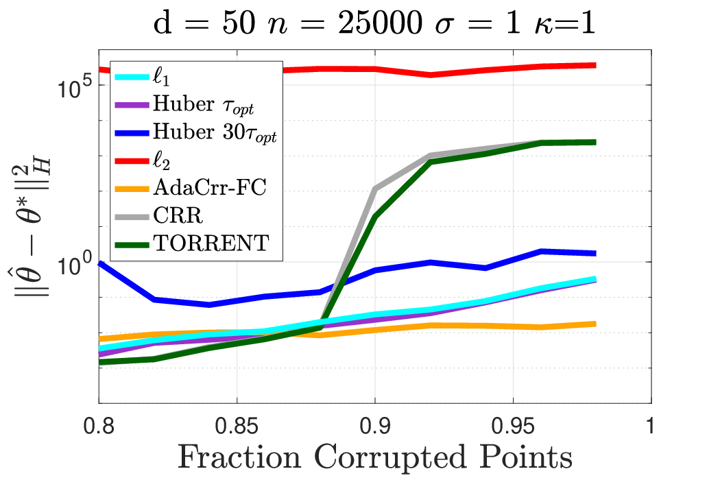
Figure 1: Online robust regression on synthetic data. Left and middle: Convergence rates for a fixed η\eta and for two different conditioning of HH. The dashed line marks the first pass over the data. Right: Estimation performance when varying the portion of corruption η\eta.

Online robust regression. We plot the convergence rate of averaged SGD on different loss functions: the ℓ1\ell_{1} loss, the ℓ2\ell_{2} loss and the Huber loss for which we consider various parameters. We also consider the AdaCRR-GD algorithm from [78]. These curves are compared to an oracle algorithm which corresponds to least-squares regression using constant step-size averaged SGD [4] and where all the corrupted points have been discarded (hence a rate of O⁡(1/(1−η)​n)O(1/(1-\eta)n) ). Since AdaCRR-GD is an offline algorithm that needs all the data to perform a single gradient step we let all algorithms perform 55 passes over the dataset (passes without replacement). In the SGD setting this corresponds to a total of 5​n5n iterations. On the plots we represent by a vertical dashed line the first effective pass over the dataset. Figure 1 in the left and middle plots are shown the experimental results for two different conditioning of HH: κ=1\kappa=1 and κ=1/d\kappa=1/d. Notice that independently of the conditioning our algorithm converges at rate O⁡(1/n)O(1/n) and almost matches the performance obtained by the oracle algorithm. Using the Huber loss leads to mixed results: if the parameter is well tuned to τo​p​t\tau_{opt} then the performance is similar to that of the ℓ1\ell_{1} loss, but if the parameter is set too large (5​τo​p​t5\tau_{opt}) then the convergence is slow and ends at a sup-optimal point, if it set too small (.2​τo​p​t.2\tau_{opt}) the convergence is slow. Indeed the Huber loss with parameter τ\tau is equivalent to τ∥⋅∥1\tau\|\cdot\|_{1} when the parameter τ\tau goes to 00. Therefore doing SGD on the Huber loss for τ→0\tau\to 0 is equivalent to performing SGD on the ℓ1\ell_{1} loss with the smaller step-size sequence (τ​γn)n≥0(\tau\gamma_{n})_{n\geq 0}. On the other hand, SGD on the ℓ2\ell_{2} loss is as predicted not competitive at all. AdaCRR-GD needs to wait a full pass before performing one single step and is in all cases much slower than SGD. Moreover notice that AdaCRR-GD is very sensitive to the conditioning of the covariance matrix: the convergence is much slower for a badly conditioned problem. Indeed in this case the convergence of the gradient descent subroutine used in the algorithm becomes sublinear and it significantly degrades the overall performance. On the other hand the performance of SGD on the ℓ1\ell_{1} loss is not affected by the conditioning.

Breakdown point and recovery guarantees. In this setting, the number of samples nn is fixed and we modify the outlier proportion η\eta. We compare our algorithm to different baselines: ℓ2\ell_{2} regression, Huber regression with a well tuned parameter τo​p​t\tau_{opt} and with a larger parameter 30​τo​p​t30\tau_{opt}, Torrent [9], CRR [9], and AdaCRR [78]. The details on their implementation are provided in the Appendix. The results are shown Figure 1, right plot. Notice that averaged SGD on the ℓ1\ell_{1} obtains comparable results to Huber regression with parameter τo​p​t\tau_{opt} and to AdaCRR, this without having any hyperparameter to tune. Note also that if the parameter of the Huber loss is set too high then the performance is degraded. The other methods are as expected not competitive.

7 Conclusion

In this paper, we studied the response robust regression problem with an oblivious adversary. We showed that by simply performing SGD with Polyak-Ruppert averaging on the ℓ1\ell_{1} loss 𝔼[|y−⟨x,θ⟩]\mathbb{E}[|y-\langle x,\ \theta\rangle] we successively recover the parameter θ∗\theta^{*} with an optimal O⁡(1/n)O(1/n) rate. The experimental results on synthetic data shows the superiority of our algorithm and its clear advantage for high-scale and online settings.
There are several interesting future directions to our work. One would be to consider other corruption models in the online setting. It would also be interesting to see if we can combine our approach with [1, 37] in order to get results in the case where θ∗\theta^{*} is sparse.

8 Broader Impact

As discussed in the introduction, the algorithm we propose can be useful in many practical applications such as : (a) detection of irrelevant measurements and systematic labelling errors [51], (b) detection of system attacks such as frauds by click bots [40] or malware recommendation rating-frauds [94], and (c) online regression with heavy-tailed noise [78].

References

  • [1] A. Agarwal, S. N. Negahban, and M. J. Wainwright. Stochastic optimization and sparse statistical recovery: Optimal algorithms for high dimensions. In NeurIPS, page 1538–1546, 2012.
  • [2] F. Bach. Adaptivity of averaged stochastic gradient descent to local strong convexity for logistic regression. J. Mach. Learn. Res., 15(1):595–627, 2014.
  • [3] F. Bach and E. Moulines. Non-asymptotic analysis of stochastic approximation algorithms for machine learning. In Advances in Neural Information Processing Systems, pages 451–459, 2011.
  • [4] F. Bach and E. Moulines. Non-strongly-convex smooth stochastic approximation with convergence rate o (1/n). In Advances in neural information processing systems, pages 773–781, 2013.
  • [5] J. T. Barron. A general and adaptive robust loss function. In CVPR, 2019.
  • [6] G. Bassett and R. Koenker. Asymptotic theory of least absolute error regression. J. Amer. Statist. Assoc., 73(363):618–622, 1978.
  • [7] A. Benveniste, P. Priouret, and M. Métivier. Adaptive Algorithms and Stochastic Approximations. Springer, 1990.
  • [8] K. Bhatia, P. Jain, P. Kamalaruban, and P. Kar. Consistent robust regression. In NeurIPS, page 2107–2116, 2017.
  • [9] K. Bhatia, P. Jain, and P. Kar. Robust regression via hard thresholding. In NeurIPS, page 721–729, 2015.
  • [10] P. Bloomfield and W. L. Steiger. Least absolute deviations, volume 6 of Progress in Probability and Statistics. 1983. Theory, applications, and algorithms.
  • [11] L. Bottou. Online algorithms and stochastic approximations. In Online Learning and Neural Networks. Cambridge University Press, Cambridge, UK, 1998.
  • [12] L. Bottou and O. Bousquet. The tradeoffs of large scale learning. In NeurIPS, pages 161–168. 2008.
  • [13] E. J. Candès and P. A. Randall. Highly robust error correction by convex programming. IEEE Trans. Inform. Theory, 54(7):2829–2840, 2008.
  • [14] N. Carlini, P. Mishra, T. Vaidya, Y. Zhang, M. Sherr, C. Shields, D. Wagner, and W. Zhou. Hidden voice commands. In 25th USENIX Security Symposium (USENIX Security 16), pages 513–530, Austin, TX, Aug. 2016. USENIX Association.
  • [15] P. Charbonnier, L. Blanc-Feraud, G. Aubert, and M. Barlaud. Two deterministic half-quadratic regularization algorithms for computed imaging. In Proceedings of 1st International Conference on Image Processing, volume 2, pages 168–172 vol.2, 1994.
  • [16] M. Charikar, J. Steinhardt, and G. Valiant. Learning from untrusted data. In Proceedings of the 49th Annual ACM SIGACT Symposium on Theory of Computing, pages 47–60, 2017.
  • [17] M. Chen, C. Gao, and Z. Ren. A general decision theory for Huber’s ϵ\epsilon-contamination model. Electron. J. Stat., 10(2):3752–3774, 2016.
  • [18] Y. Chen, C. Caramanis, and S. Mannor. Robust sparse regression under adversarial corruption. In ICML, volume 28 of PMLR, pages 774–782, 2013.
  • [19] Y. Chen and A. S. Dalalyan. Fused sparsity and robust estimation for linear models with unknown variance. In NeurIPS, page 1259–1267, 2012.
  • [20] A. Dalalyan and P. Thompson. Outlier-robust estimation of a sparse linear model using ℓ1\ell_{1}-penalized huber’s m-estimator. In NeurIPS, pages 13188–13198. 2019.
  • [21] I. Diakonikolas, G. Kamath, D. Kane, J. Li, J. Steinhardt, and A. Stewart. Sever: A robust meta-algorithm for stochastic optimization. In Proceedings of the 36th International Conference on Machine Learning, volume 97 of Proceedings of Machine Learning Research, pages 1596–1606. PMLR, 09–15 Jun 2019.
  • [22] I. Diakonikolas, G. Kamath, D. M. Kane, J. Li, A. Moitra, and A. Stewart. Robust estimators in high dimensions without the computational intractability. In Foundations of Computer Science (FOCS), 2016.
  • [23] I. Diakonikolas, G. Kamath, D. M. Kane, J. Li, A. Moitra, and A. Stewart. Being robust (in high dimensions) can be practical. In Proceedings of the 34th International Conference on Machine Learning, volume 70 of Proceedings of Machine Learning Research, pages 999–1008. PMLR, 2017.
  • [24] I. Diakonikolas, G. Kamath, D. M. Kane, J. Li, A. Moitra, and A. Stewart. Robustly learning a Gaussian: Getting optimal error, efficiently. In Proceedings of the Twenty-Ninth Annual ACM-SIAM Symposium on Discrete Algorithms, pages 2683–2702. SIAM, 2018.
  • [25] I. Diakonikolas and D. M. Kane. Recent advances in algorithmic high-dimensional robust statistics. arXiv preprint arXiv:1911.05911, 2019.
  • [26] I. Diakonikolas, D. M. Kane, and A. Stewart. List-decodable robust mean estimation and learning mixtures of spherical Gaussians. In Proceedings of the 50th Annual ACM SIGACT Symposium on Theory of Computing, pages 1047–1060, 2018.
  • [27] I. Diakonikolas, W. Kong, and A. Stewart. Efficient algorithms and lower bounds for robust linear regression. In SODA, page 2745–2754, 2019.
  • [28] D. Donoho and P. J. Huber. The notion of breakdown point. In A Festschrift for Erich L. Lehmann, Wadsworth Statist./Probab. Ser., pages 157–184. 1983.
  • [29] D. Donoho and A. Montanari. High dimensional robust M-estimation: asymptotic variance via approximate message passing. Probab. Theory Related Fields, 166(3-4):935–969, 2016.
  • [30] J. C. Duchi, P. L. Bartlett, and M. J. Wainwright. Randomized smoothing for stochastic optimization. SIAM J. Optim., 22(2):674–701, 2012.
  • [31] F. Edgeworth. On a new method of reducing observations relating to several quantities. The London, Edinburgh, and Dublin Philosophical Magazine and Journal of Science, 25(154):184–191, 1888.
  • [32] K. Eykholt, I. Evtimov, E. Fernandes, B. Li, A. Rahmati, C. Xiao, A. Prakash, T. Kohno, and D. Song. Robust physical-world attacks on deep learning visual classification. In 2018 IEEE/CVF Conference on Computer Vision and Pattern Recognition, pages 1625–1634, 2018.
  • [33] M. A. Fischler and R. C. Bolles. Random sample consensus: A paradigm for model fitting with applications to image analysis and automated cartography. Commun. ACM, 24(6):381–395, June 1981.
  • [34] N. Flammarion and F. Bach. Stochastic composite least-squares regression with convergence rate o⁡(1/n)o(1/n). In COLT, volume 65 of Proceedings of Machine Learning Research, pages 831–875, 07–10 Jul 2017.
  • [35] B. Fritsch, V. and[Da Mota], E. Loth, G. Varoquaux, T. Banaschewski, G. Barker, A. Bokde, R. Bruehl, B. Butzek, P. Conrod, H. Flor, H. Garavan, H. Lemaitre, K. Mann, F. Nees, T. Paus, D. J. Schad, G. Schuemann, V. Frouin, J.-B. Poline, and B. Thirion. Robust regression for large-scale neuroimaging studies. NeuroImage, 111:431 – 441, 2015.
  • [36] J.-J. Fuchs. An inverse problem approach to robust regression. In Proceedings of ICASSP, page 1809–1812, 1999.
  • [37] P. Gaillard and O. Wintenberger. Sparse accelerated exponential weights. In AISTAT, volume 54 of PMLT, pages 75–82, 2017.
  • [38] C. Gao. Robust regression via mutivariate regression depth. Bernoulli, 26(2):1139–1170, 2020.
  • [39] I. Goodfellow, P. McDaniel, and N. Papernot. Making machine learning robust against adversarial inputs. Commun. ACM, 61(7):56–66, June 2018.
  • [40] H. Haddadi. Fighting online click-fraud using bluff ads. SIGCOMM Comput. Commun. Rev., 40(2):21–25, Apr. 2010.
  • [41] F. R. Hampel. A general qualitative definition of robustness. Ann. Math. Statist., 42:1887–1896, 1971.
  • [42] F. R. Hampel, E. M. Ronchetti, P. J. Rousseeuw, and W. A. Stahel. Robust Statistics: the Approach Based on Influence Functions, volume 196. John Wiley & Sons, 2011.
  • [43] N. J. A. Harvey, C. Liaw, Y. Plan, and S. Randhawa. Tight analyses for non-smooth stochastic gradient descent. In COLT, volume 99 of PMLR, pages 1579–1613, 2019.
  • [44] S. Hopkins and J. Li. Mixture models, robustness, and sum of squares proofs. In Proceedings of the 50th Annual ACM SIGACT Symposium on Theory of Computing, pages 1021–1034. ACM, 2018.
  • [45] P. J. Huber. Robust estimation of a location parameter. Ann. Math. Statist., 35:73–101, 1964.
  • [46] P. J. Huber. Robust regression: asymptotics, conjectures and Monte Carlo. Ann. Statist., 1:799–821, 1973.
  • [47] S. Karmalkar and E. Price. Compressed sensing with adversarial sparse noise via l1 regression. In SOSA, volume 69, pages 19:1–19:19, 2018.
  • [48] A. Klivans, P. K. Kothari, and R. Meka. Efficient algorithms for outlier-robust regression. In Proceedings of the 31st Conference On Learning Theory, volume 75 of Proceedings of Machine Learning Research, pages 1420–1430. PMLR, 2018.
  • [49] P. K. Kothari, J. Steinhardt, and D. Steurer. Robust moment estimation and improved clustering via sum of squares. In Proceedings of the 50th Annual ACM SIGACT Symposium on Theory of Computing, pages 1035–1046, 2018.
  • [50] K. A. Lai, A. B. Rao, and S. Vempala. Agnostic estimation of mean and covariance. In Foundations of Computer Science (FOCS), 2016.
  • [51] J. N. Laska, M. A. Davenport, and R. G. Baraniuk. Exact signal recovery from sparsely corrupted measurements through the pursuit of justice. In 2009 Conference Record of the Forty-Third Asilomar Conference on Signals, Systems and Computers, pages 1556–1560, 2009.
  • [52] F. C. Leone, L. S. Nelson, and R. B. Nottingham. The folded normal distribution. Technometrics, 3:543–550, 1961.
  • [53] L. Liu, T. Li, and C. Caramanis. High dimensional robust mm-estimation: Arbitrary corruption and heavy tails, 2019.
  • [54] L. Liu, Y. Shen, T. Li, and C. Caramanis. High dimensional robust sparse regression. In AISTAT, PMLR, 2020.
  • [55] P.-L. Loh. Statistical consistency and asymptotic normality for high-dimensional robust MM-estimators. Ann. Statist., 45(2):866–896, 2017.
  • [56] R. A. Maronna and V. J. Yohai. Asymptotic behavior of general MM-estimates for regression and scale with random carriers. Z. Wahrsch. Verw. Gebiete, 58(1):7–20, 1981.
  • [57] H. B. McMahan, G. Holt, D. Sculley, M. Young, D. Ebner, J. Grady, L. Nie, T. Phillips, E. Davydov, D. Golovin, et al. Ad click prediction: a view from the trenches. In Proceedings of the 19th ACM SIGKDD international conference on Knowledge discovery and data mining, pages 1222–1230, 2013.
  • [58] B. Mukhoty, G. Gopakumar, P. Jain, and P. Kar. Globally-convergent iteratively reweighted least squares for robust regression problems. In AISTAT, volume 89 of PMLR, pages 313–322, 2019.
  • [59] A. Nemirovski, A. Juditsky, G. Lan, and A. Shapiro. Robust stochastic approximation approach to stochastic programming. SIAM J. Optim., 19(4):1574–1609, 2008.
  • [60] A. S. Nemirovsky and D. B. Yudin. Problem Complexity and Method Efficiency in Optimization. Wiley-Interscience Series in Discrete Mathematics. John Wiley & Sons, 1983.
  • [61] Y. Nesterov and V. Spokoiny. Random gradient-free minimization of convex functions. Found. Comput. Math., 17(2):527–566, 2017.
  • [62] N. H. Nguyen and T. D. Tran. Exact recoverability from dense corrupted observations via ℓ1\ell_{1}-minimization. IEEE Trans. Inform. Theory, 59(4):2017–2035, 2013.
  • [63] N. H. Nguyen and T. D. Tran. Robust Lasso with missing and grossly corrupted observations. IEEE Trans. Inform. Theory, 59(4):2036–2058, 2013.
  • [64] D. Pollard. Asymptotics for least absolute deviation regression estimators. Econometric Theory, 7(2):186–199, 1991.
  • [65] B. T. Polyak. A new method of stochastic approximation type. Avtomatika i Telemekhanika, 51(7):98–107, 1990.
  • [66] B. T. Polyak and A. B. Juditsky. Acceleration of stochastic approximation by averaging. SIAM J. Control Optim., 30(4):838–855, 1992.
  • [67] A. Prasad, A. S. Suggala, S. Balakrishnan, and P. Ravikumar. Robust estimation via robust gradient estimation, 2018.
  • [68] H. Robbins and S. Monro. A stochastic approxiation method. Ann. Math. Statist, 22(3):400–407, 1951.
  • [69] P. J. Rousseeuw. Least median of squares regression. J. Amer. Statist. Assoc., 79(388):871–880, 1984.
  • [70] P. J. Rousseeuw. Multivariate estimation with high breakdown point. In Mathematical statistics and applications, pages 283–297. 1985.
  • [71] P. J. Rousseeuw. An application of L1L_{1} to astronomy. In Statistical data analysis based on the L1L_{1}-norm and related methods (Neuchâtel, 1987), pages 437–445. North-Holland, Amsterdam, 1987.
  • [72] P. J. Rousseeuw and K. V. Driessen. A fast algorithm for the minimum covariance determinant estimator. Technometrics, 41(3):212–223, 1999.
  • [73] D. Ruppert. Efficient estimations from a slowly convergent robbins-monro process. Technical report, Cornell University Operations Research and Industrial Engineering, 1988.
  • [74] O. Shamir and T. Zhang. Stochastic gradient descent for non-smooth optimization: Convergence results and optimal averaging schemes. In ICML, volume 28 of PMLR, pages 71–79, 2013.
  • [75] O. Stegle, D. J. C. Fallert, S. V. andMacKay, and S. Brage. Gaussian process robust regression for noisy heart rate data. IEEE Transactions on Biomedical Engineering, 55(9):2143–2151, 2008.
  • [76] J. Steinhardt, M. Charikar, and G. Valiant. Resilience: A Criterion for Learning in the Presence of Arbitrary Outliers. In 9th Innovations in Theoretical Computer Science Conference (ITCS 2018), volume 94, 2018.
  • [77] C. Studer, P. Kuppinger, G. Pope, and H. Bolcskei. Recovery of sparsely corrupted signals. IEEE Transactions on Information Theory, 58(5):3115–3130, 2012.
  • [78] A. S. Suggala, K. Bhatia, P. Ravikumar, and P. Jain. Adaptive hard thresholding for near-optimal consistent robust regression. In COLT, volume 99 of PMLR, pages 2892–2897, 2019.
  • [79] E. Tsakonas, J. Jaldén, N. D. Sidiropoulos, and B. Ottersten. Convergence of the huber regression m-estimate in the presence of dense outliers. IEEE Signal Processing Letters, 21(10):1211–1214, 2014.
  • [80] A. B. Tsybakov. Introduction to Nonparametric Estimation. Springer Series in Statistics. Springer, 2009.
  • [81] J. W. Tukey. A survey of sampling from contaminated distributions. In Contributions to probability and statistics, pages 448–485. Stanford Univ. Press, Stanford, Calif., 1960.
  • [82] S. A. van de Geer. Empirical Processes in M-Estimation, volume 6 of Cambridge Series in Statistical and Probabilistic Mathematics. Cambridge University Press, Cambridge, 2000.
  • [83] A. W. van der Vaart. Asymptotic statistics, volume 3 of Cambridge Series in Statistical and Probabilistic Mathematics. Cambridge University Press, Cambridge, 1998.
  • [84] J. M. Wooldridge. A unified approach to robust, regression-based specification tests. Econometric Theory, 6(1):17–43, 1990.
  • [85] J. Wright and Y. Ma. Dense error correction via ℓ1\ell^{1}-minimization. IEEE Trans. Inform. Theory, 56(7):3540–3560, 2010.
  • [86] Y. Wright, A. Y. Yang, A. Ganesh, S. S. Sastry, and Y. Ma. Robust face recognition via sparse representation. IEEE Transactions on Pattern Analysis and Machine Intelligence, 31(2):210–227, 2009.
  • [87] A. Yang, S. Sastry, A. Ganesh, and Y. Ma. Fast l1-minimization algorithms and an application in robust face recognition: A review. In International Conference on Image Processin, 2010.
  • [88] M. K. S. Yeung, J. Tegnér, and J. J. Collins. Reverse engineering gene networks using singular value decomposition and robust regression. Proceedings of the National Academy of Sciences, 99(9):6163–6168, 2002.
  • [89] Yin Wang, C. Dicle, M. Sznaier, and O. Camps. Self scaled regularized robust regression. In 2015 IEEE Conference on Computer Vision and Pattern Recognition (CVPR), pages 3261–3269, 2015.
  • [90] V. J. Yohai. High breakdown-point and high efficiency robust estimates for regression. Ann. Statist., 15(2):642–656, 1987.
  • [91] A. Zaman, P. J. Rousseeuw, and M. Orhan. Econometric applications of high-breakdown robust regression techniques. Economics Letters, 71(1):1–8, 2001.
  • [92] T. Zhang. Solving large scale linear prediction problems using stochastic gradient descent algorithms. In Proceedings of the Conference on Machine Learning (ICML), 2004.
  • [93] W.-X. Zhou, K. Bose, J. Fan, and H. Liu. A new perspective on robust MM-estimation: finite sample theory and applications to dependence-adjusted multiple testing. Ann. Statist., 46(5):1904–1931, 2018.
  • [94] H. Zhu, H. Xiong, Y. Ge, and E. Chen. Discovery of ranking fraud for mobile apps. IEEE Transactions on Knowledge and Data Engineering, 27(1):74–87, 2015.

Appendix A Higher-order moment bounds

In this section we prove classical moment bounds on the SGD iterates following eq. 2 with the decreasing step-size sequence γn=γ0/n\gamma_{n}=\gamma_{0}/\sqrt{n}. The following results are highly inspired from [3], [2] and [74] with the slight technical differences that: the iterates are not bounded since no projection is used, the stochastic gradients are not almost surely bounded and a decreasing step-size is considered.

  • •

    Lemma 8 we give second and fourth moment bounds on ‖θn−θ∗‖\left\lVert\theta_{n}-\theta^{*}\right\rVert.

  • •

    Lemma 9 we give first and second moment bounds on f⁡(θ¯n)−f⁡(θ∗)f(\bar{\theta}_{n})-f(\theta^{*}).

  • •

    Lemma 10 we give first and second moment bounds on f⁡(θn)−f⁡(θ∗)f(\theta_{n})-f(\theta^{*}).

We start by providing second and fourth moment bounds on ‖θn−θ∗‖\left\lVert\theta_{n}-\theta^{*}\right\rVert in the following lemma.

Lemma 8.

Let (A.1, A.2, A.3, A.4) hold and consider the SGD iterates following Eq. (2). Assume γn=γ0n\gamma_{n}=\frac{\gamma_{0}}{\sqrt{n}}. Then:

𝔼⁡[‖θn−θ∗‖2]≤(‖θ0−θ∗‖2+γ02​R2​ln⁡(e​n)):=Cn,\mathbb{E}\left[\left\lVert\theta_{n}-\theta^{*}\right\rVert^{2}\right]\leq\left(\left\lVert\theta_{0}-\theta^{*}\right\rVert^{2}+\gamma_{0}^{2}R^{2}\ln(en)\right):=C_{n},
𝔼⁡[‖θn−θ∗‖4]≤(‖θ0−θ∗‖2+4​γ02​R2​ln⁡(e​n))2:=Dn.\mathbb{E}\left[\left\lVert\theta_{n}-\theta^{*}\right\rVert^{4}\right]\leq\left(\left\lVert\theta_{0}-\theta^{*}\right\rVert^{2}+4\gamma_{0}^{2}R^{2}\ln(en)\right)^{2}:=D_{n}.
Proof.

Starting from the definition of the SGD recursion eq. 2 we have:

θn=θn−1−γn​fn′​(θn−1),\theta_{n}=\theta_{n-1}-\gamma_{n}f^{\prime}_{n}(\theta_{n-1}), (3)

and get the classical recursion:

‖θn−θ∗‖2=‖θn−1−θ∗‖2−2​γn​⟨fn′​(θn−1),θn−1−θ∗⟩+γn2​‖fn′​(θn−1)‖2.\left\lVert\theta_{n}-\theta^{*}\right\rVert^{2}=\left\lVert\theta_{n-1}-\theta^{*}\right\rVert^{2}-2\gamma_{n}\langle f^{\prime}_{n}(\theta_{n-1}),\theta_{n-1}-\theta^{*}\rangle+\gamma_{n}^{2}\left\lVert f^{\prime}_{n}(\theta_{n-1})\right\rVert^{2}. (4)

Second moment bound.

We take the conditional expectation w.r.t the filtration ℱn−1=σ⁡((xi,yi)1≤i≤n−1)\mathcal{F}_{n-1}=\sigma((x_{i},y_{i})_{1\leq i\leq n-1}):

𝔼⁡[‖θn−θ∗‖2|ℱn−1]=‖θn−1−θ∗‖2−2​γn​⟨f′​(θn−1),θn−1−θ∗⟩+γn2​‖fn′​(θn−1)‖2,\mathbb{E}\left[\left\lVert\theta_{n}-\theta^{*}\right\rVert^{2}|\mathcal{F}_{n-1}\right]=\left\lVert\theta_{n-1}-\theta^{*}\right\rVert^{2}-2\gamma_{n}\langle f^{\prime}(\theta_{n-1}),\theta_{n-1}-\theta^{*}\rangle+\gamma_{n}^{2}\left\lVert f^{\prime}_{n}(\theta_{n-1})\right\rVert^{2},

taking the full expectation and using that by convexity of ff, ⟨f′​(θn−1),θn−1−θ∗⟩≥0\langle f^{\prime}(\theta_{n-1}),\theta_{n-1}-\theta^{*}\rangle\geq 0, we obtain:

𝔼⁡[‖θn−θ∗‖2]≤𝔼⁡[‖θn−1−θ∗‖2]+γn2​R2≤‖θ0−θ∗‖2+γ02​R2​∑k=1nk−1≤‖θ0−θ∗‖2+γ02​R2​ln⁡(e​n).\mathbb{E}\left[\left\lVert\theta_{n}-\theta^{*}\right\rVert^{2}\right]\leq\mathbb{E}\left[\left\lVert\theta_{n-1}-\theta^{*}\right\rVert^{2}\right]+\gamma_{n}^{2}R^{2}\leq\left\lVert\theta_{0}-\theta^{*}\right\rVert^{2}+\gamma_{0}^{2}R^{2}\sum_{k=1}^{n}k^{-1}\leq\left\lVert\theta_{0}-\theta^{*}\right\rVert^{2}+\gamma_{0}^{2}R^{2}\ln(en).

Fourth moment bound.

For the fourth-order moment bound, we take the square of Eq. (4):

‖θn−θ∗‖4=\displaystyle\left\lVert\theta_{n}-\theta^{*}\right\rVert^{4}= ‖θn−1−θ∗‖4+4​γn2​⟨fn′​(θn−1),θn−1−θ∗⟩2+γn4​‖fn′​(θn−1)‖4\displaystyle\left\lVert\theta_{n-1}-\theta^{*}\right\rVert^{4}+4\gamma_{n}^{2}\langle f^{\prime}_{n}(\theta_{n-1}),\theta_{n-1}-\theta^{*}\rangle^{2}+\gamma_{n}^{4}\left\lVert f^{\prime}_{n}(\theta_{n-1})\right\rVert^{4}
−4​γn​⟨fn′​(θn−1),θn−1−θ∗⟩​‖θn−1−θ∗‖2−4​γn3​⟨fn′​(θn−1),θn−1−θ∗⟩​‖fn′​(θn−1)‖2\displaystyle-4\gamma_{n}\langle f^{\prime}_{n}(\theta_{n-1}),\theta_{n-1}-\theta^{*}\rangle\left\lVert\theta_{n-1}-\theta^{*}\right\rVert^{2}-4\gamma_{n}^{3}\langle f^{\prime}_{n}(\theta_{n-1}),\theta_{n-1}-\theta^{*}\rangle\left\lVert f^{\prime}_{n}(\theta_{n-1})\right\rVert^{2}
+2​γn2​‖θn−1−θ∗‖2​‖fn′​(θn−1)‖2.\displaystyle+2\gamma_{n}^{2}\left\lVert\theta_{n-1}-\theta^{*}\right\rVert^{2}\left\lVert f^{\prime}_{n}(\theta_{n-1})\right\rVert^{2}.

Taking the conditional expectation:

𝔼⁡[‖θn−θ∗‖4|ℱn−1]=\displaystyle\mathbb{E}\left[\left\lVert\theta_{n}-\theta^{*}\right\rVert^{4}|\mathcal{F}_{n-1}\right]= ‖θn−1−θ∗‖4+4γn2⟨𝔼[fn′(θn−1),θn−1−θ∗⟩2|ℱn]+γn4𝔼[‖fn′(θn−1)‖4|ℱn]\displaystyle\left\lVert\theta_{n-1}-\theta^{*}\right\rVert^{4}+4\gamma_{n}^{2}\langle\mathbb{E}\left[f^{\prime}_{n}(\theta_{n-1}),\theta_{n-1}-\theta^{*}\rangle^{2}|\mathcal{F}_{n}\right]+\gamma_{n}^{4}\mathbb{E}\left[\left\lVert f^{\prime}_{n}(\theta_{n-1})\right\rVert^{4}|\mathcal{F}_{n}\right]
−4​γn​⟨f′​(θn−1),θn−1−θ∗⟩​‖θn−1−θ∗‖2−4​γn3​𝔼​[⟨fn′​(θn−1),θn−1−θ∗⟩​‖fn′​(θn−1)‖2|ℱn]\displaystyle-4\gamma_{n}\langle f^{\prime}(\theta_{n-1}),\theta_{n-1}-\theta^{*}\rangle\left\lVert\theta_{n-1}-\theta^{*}\right\rVert^{2}-4\gamma_{n}^{3}\mathbb{E}\left[\langle f^{\prime}_{n}(\theta_{n-1}),\theta_{n-1}-\theta^{*}\rangle\left\lVert f^{\prime}_{n}(\theta_{n-1})\right\rVert^{2}|\mathcal{F}_{n}\right]
+2​γn2​‖θn−1−θ∗‖2​𝔼​[‖fn′​(θn−1)‖2|ℱn]\displaystyle+2\gamma_{n}^{2}\left\lVert\theta_{n-1}-\theta^{*}\right\rVert^{2}\mathbb{E}\left[\left\lVert f^{\prime}_{n}(\theta_{n-1})\right\rVert^{2}|\mathcal{F}_{n}\right]
≤\displaystyle\leq ‖θn−1−θ∗‖4+6​γn2​R2​‖θn−1−θ∗‖2+3​γn4​(R2)2+2​γn2​‖θn−1−θ∗‖2​R2.\displaystyle\left\lVert\theta_{n-1}-\theta^{*}\right\rVert^{4}+6\gamma_{n}^{2}R^{2}\left\lVert\theta_{n-1}-\theta^{*}\right\rVert^{2}+3\gamma_{n}^{4}(R^{2})^{2}+2\gamma_{n}^{2}\left\lVert\theta_{n-1}-\theta^{*}\right\rVert^{2}R^{2}.

Taking the full expectation yields to

𝔼⁡[‖θn−θ∗‖4]≤\displaystyle\mathbb{E}\left[\left\lVert\theta_{n}-\theta^{*}\right\rVert^{4}\right]\leq 𝔼⁡[‖θn−1−θ∗‖4]+8​γn2​R2​𝔼​[‖θn−1−θ∗‖2]+3​γn4​(R2)2\displaystyle\mathbb{E}\left[\left\lVert\theta_{n-1}-\theta^{*}\right\rVert^{4}\right]+8\gamma_{n}^{2}R^{2}\mathbb{E}\left[\left\lVert\theta_{n-1}-\theta^{*}\right\rVert^{2}\right]+3\gamma_{n}^{4}(R^{2})^{2}
≤\displaystyle\leq 𝔼⁡[‖θn−1−θ∗‖4]+8​γn2​R2​Dn−1+3​γn4​(R2)2\displaystyle\mathbb{E}\left[\left\lVert\theta_{n-1}-\theta^{*}\right\rVert^{4}\right]+8\gamma_{n}^{2}R^{2}D_{n-1}+3\gamma_{n}^{4}(R^{2})^{2}
≤\displaystyle\leq ‖θ0−θ∗‖4+8​γ02​R2​∑k=1n‖θ0−θ∗‖2+γ02​R2​ln⁡(e⁡(k−1))k+3​γ04​(R2)2​∑k=1n1k2\displaystyle{\left\lVert\theta_{0}-\theta^{*}\right\rVert^{4}}+8\gamma_{0}^{2}R^{2}\sum_{k=1}^{n}\frac{\left\lVert\theta_{0}-\theta^{*}\right\rVert^{2}+\gamma_{0}^{2}R^{2}\ln(e(k-1))}{k}+3\gamma_{0}^{4}(R^{2})^{2}\sum_{k=1}^{n}\frac{1}{k^{2}}
≤\displaystyle\leq ‖θ0−θ∗‖4+8​γ02​R2​(‖θ0−θ∗‖2+γ02​R2​ln⁡(e​n))​ln⁡(e​n)+3​γ04​(R2)2​π2/6\displaystyle{\left\lVert\theta_{0}-\theta^{*}\right\rVert^{4}}+8\gamma_{0}^{2}R^{2}(\left\lVert\theta_{0}-\theta^{*}\right\rVert^{2}+\gamma_{0}^{2}R^{2}\ln(en))\ln(en)+3\gamma_{0}^{4}(R^{2})^{2}\pi^{2}/6
≤\displaystyle\leq ‖θ0−θ∗‖4+8​γ02​ln⁡(e​n)​R2​‖θ0−θ∗‖2+γ04​ln⁡(e​n)​(R2)2​(8​ln⁡(e​n)+π2/3)\displaystyle\left\lVert\theta_{0}-\theta^{*}\right\rVert^{4}+8\gamma_{0}^{2}\ln(en)R^{2}\left\lVert\theta_{0}-\theta^{*}\right\rVert^{2}+\gamma_{0}^{4}\ln(en)(R^{2})^{2}(8\ln(en)+\pi^{2}/3)
≤\displaystyle\leq (‖θ0−θ∗‖2+4​γ02​R2​ln⁡(e​n))2.\displaystyle\left(\left\lVert\theta_{0}-\theta^{*}\right\rVert^{2}+4\gamma_{0}^{2}R^{2}\ln(en)\right)^{2}.

∎ We then give first and second moment bounds on the function value evaluated in the averaged iterate: f⁡(θ¯n)−f⁡(θ∗)f(\bar{\theta}_{n})-f(\theta^{*}).

Lemma 9.

Let (A.1, A.2, A.3, A.4) hold and consider the SGD iterates following Eq. (2). Assume γn=γ0n\gamma_{n}=\frac{\gamma_{0}}{\sqrt{n}}. Then:

𝔼⁡[f⁡(θ¯n)]−f⁡(θ∗)≤1n​∑k=0n−1𝔼⁡[⟨f′​(θk),θk−θ∗⟩]≤1n​[‖θ0−θ∗‖2γ0+2​γ0​R2​ln⁡(e​n)],\mathbb{E}\left[f(\bar{\theta}_{n})\right]-f(\theta^{*})\leq\frac{1}{n}\sum_{k=0}^{n-1}\mathbb{E}\left[\langle f^{\prime}(\theta_{k}),\theta_{k}-\theta^{*}\rangle\right]\leq\frac{1}{\sqrt{n}}\left[\frac{\left\lVert\theta_{0}-\theta^{*}\right\rVert^{2}}{\gamma_{0}}+2\gamma_{0}R^{2}\ln(en)\right],
𝔼⁡[(f⁡(θ¯n)−f⁡(θ∗))2]≤𝔼⁡[(1n​∑k=0n−1⟨f′​(θk),θk−θ∗⟩)2]≤ln⁡(e​n)n​[‖θ0−θ∗‖2γ0+6​γ0​R2​ln⁡(e​n)]2.\mathbb{E}\left[\left(f(\bar{\theta}_{n})-f(\theta^{*})\right)^{2}\right]\leq\mathbb{E}\left[\left(\frac{1}{n}\sum_{k=0}^{n-1}\langle f^{\prime}(\theta_{k}),\theta_{k}-\theta^{*}\rangle\right)^{2}\right]\leq\frac{\ln(en)}{n}\left[\frac{\|\theta_{0}-\theta^{*}\|^{2}}{\gamma_{0}}+6\gamma_{0}R^{2}\ln(en)\right]^{2}.
Proof.

Rearranging Eq. (4) we have:

2​⟨f′​(θn−1),θn−1−θ∗⟩=γn−1​‖θn−1−θ∗‖2−γn−1​‖θn−θ∗‖2+γn​Nn+Mn,2\langle f^{\prime}(\theta_{n-1}),\theta_{n-1}-\theta^{*}\rangle=\gamma_{n}^{-1}\left\lVert\theta_{n-1}-\theta^{*}\right\rVert^{2}-\gamma_{n}^{-1}\left\lVert\theta_{n}-\theta^{*}\right\rVert^{2}+\gamma_{n}N_{n}+M_{n},

where we denote by Nn:=‖fn′​(θn−1)‖2N_{n}:=\left\lVert f^{\prime}_{n}(\theta_{n-1})\right\rVert^{2} and Mn:=2​⟨f′​(θn−1)−fn′​(θn−1),θn−1−θ∗⟩M_{n}:=2\langle f^{\prime}(\theta_{n-1})-f^{\prime}_{n}(\theta_{n-1}),\theta_{n-1}-\theta^{*}\rangle which both satisfy 𝔼⁡[Nn]≤R2\mathbb{E}\left[N_{n}\right]\leq R^{2}, 𝔼⁡[Mn]=0\mathbb{E}\left[M_{n}\right]=0 and 𝔼⁡[Mn2]≤8​𝔼​[‖θn−1−θ∗‖2]​R2\mathbb{E}\left[M_{n}^{2}\right]\leq 8\mathbb{E}\left[\left\lVert\theta_{n-1}-\theta^{*}\right\rVert^{2}\right]R^{2}.

Taking the sum of the previous equality for k=1k=1 to k=nk=n, we obtain:

2​∑k=0n−1⟨f′​(θk),θk−θ∗⟩=γ0−1​‖θ0−θ∗‖2−γn−1​‖θn−θ∗‖2+∑k=1n−1‖θk−θ∗‖2(γk+1−1−γk−1)+∑k=1n(γkNk+Mk).2\sum_{k=0}^{n-1}\langle f^{\prime}(\theta_{k}),\theta_{k}-\theta^{*}\rangle=\gamma_{0}^{-1}\left\lVert\theta_{0}-\theta^{*}\right\rVert^{2}-\gamma_{n}^{-1}\left\lVert\theta_{n}-\theta^{*}\right\rVert^{2}\\ +\sum_{k=1}^{n-1}\left\lVert\theta_{k}-\theta^{*}\right\rVert^{2}(\gamma_{k+1}^{-1}-\gamma_{k}^{-1})+\sum_{k=1}^{n}(\gamma_{k}N_{k}+M_{k}). (5)

First moment bound.

The first result is obtained by directly taking the expectation, using lemma 8 to bound 𝔼⁡[‖θk−θ∗‖2]\mathbb{E}\left[\left\lVert\theta_{k}-\theta^{*}\right\rVert^{2}\right] and using the classical inequality ∑k=1nk−1≤2​n\sum_{k=1}^{n}\sqrt{k}^{-1}\leq 2\sqrt{n}:

2​∑k=0n−1𝔼⁡[⟨f′​(θk),θk−θ∗⟩]\displaystyle 2\sum_{k=0}^{n-1}\mathbb{E}\left[\langle f^{\prime}(\theta_{k}),\theta_{k}-\theta^{*}\rangle\right] =γ0−1​‖θ0−θ∗‖2−γn−1​𝔼​[‖θn−θ∗‖2]+∑k=1n−1𝔼⁡[‖θk−θ∗‖2]​(γk+1−1−γk−1)\displaystyle=\gamma_{0}^{-1}\left\lVert\theta_{0}-\theta^{*}\right\rVert^{2}-\gamma_{n}^{-1}\mathbb{E}\left[\left\lVert\theta_{n}-\theta^{*}\right\rVert^{2}\right]+\sum_{k=1}^{n-1}\mathbb{E}\left[\left\lVert\theta_{k}-\theta^{*}\right\rVert^{2}\right](\gamma_{k+1}^{-1}-\gamma_{k}^{-1})
+∑k=1nγk𝔼[Nk]\displaystyle\qquad+\sum_{k=1}^{n}\gamma_{k}\mathbb{E}\left[N_{k}\right]
≤γ0−1​‖θ0−θ∗‖2−γn−1​𝔼​[‖θn−θ∗‖2]+Cn−1​∑k=1n−1(γk+1−1−γk−1)+R2​γ0​∑k=1nk−1\displaystyle\leq\gamma_{0}^{-1}\left\lVert\theta_{0}-\theta^{*}\right\rVert^{2}-\gamma_{n}^{-1}\mathbb{E}\left[\left\lVert\theta_{n}-\theta^{*}\right\rVert^{2}\right]+C_{n-1}\sum_{k=1}^{n-1}(\gamma_{k+1}^{-1}-\gamma_{k}^{-1})+R^{2}\gamma_{0}\sum_{k=1}^{n}\sqrt{k}^{-1}
≤γ0−1​‖θ0−θ∗‖2+γn−1​Cn−1+2​R2​γ0​n\displaystyle\leq\gamma_{0}^{-1}\left\lVert\theta_{0}-\theta^{*}\right\rVert^{2}+\gamma_{n}^{-1}C_{n-1}+2R^{2}\gamma_{0}\sqrt{n}
≤γ0−1​‖θ0−θ∗‖2+γn−1​(‖θ0−θ∗‖2+γ02​R2​ln⁡(e​n))+2​R2​γ0​n\displaystyle\leq\gamma_{0}^{-1}\left\lVert\theta_{0}-\theta^{*}\right\rVert^{2}+\gamma_{n}^{-1}\left(\left\lVert\theta_{0}-\theta^{*}\right\rVert^{2}+\gamma_{0}^{2}R^{2}\ln(en)\right)+2R^{2}\gamma_{0}\sqrt{n}
≤n​[2​‖θ0−θ∗‖2γ0+4​γ0​R2​ln⁡(e​n)].\displaystyle\leq\sqrt{n}\left[\frac{2\left\lVert\theta_{0}-\theta^{*}\right\rVert^{2}}{\gamma_{0}}+4\gamma_{0}R^{2}\ln(en)\right].

Second moment bound.

Notice that γk+1−1−γk−1=1γ0​(k+1+k)≤1/(2​γ0​k)\gamma_{k+1}^{-1}-\gamma_{k}^{-1}=\frac{1}{\gamma_{0}(\sqrt{k+1}+\sqrt{k})}\leq 1/(2\gamma_{0}\sqrt{k}). To obtain the second-moment bound, we define An:=γ0−1​‖θ0−θ∗‖2+∑k=1n−1‖θk−θ∗‖22​γ0​k+∑k=1n(γk​Nk+Mk)A_{n}:=\gamma_{0}^{-1}\left\lVert\theta_{0}-\theta^{*}\right\rVert^{2}+\sum_{k=1}^{n-1}\frac{\left\lVert\theta_{k}-\theta^{*}\right\rVert^{2}}{2\gamma_{0}\sqrt{k}}+\sum_{k=1}^{n}(\gamma_{k}N_{k}+M_{k}) which satisfies the recursion formula for A0=‖θ0−θ∗‖22​γ0A_{0}=\frac{\left\lVert\theta_{0}-\theta^{*}\right\rVert^{2}}{2\gamma_{0}}:

An=An−1+‖θn−1−θ∗‖22​γ0​n+(γn​Nn+Mn).A_{n}=A_{n-1}+\frac{\left\lVert\theta_{n-1}-\theta^{*}\right\rVert^{2}}{2\gamma_{0}\sqrt{n}}+(\gamma_{n}N_{n}+M_{n}).

When proving the first moment bound we showed by induction that 𝔼⁡[An]≤n​[2​‖θ0−θ∗‖2γ0+4​γ0​R2​ln⁡(e​n)]\mathbb{E}\left[A_{n}\right]\leq\sqrt{n}[\frac{2\left\lVert\theta_{0}-\theta^{*}\right\rVert^{2}}{\gamma_{0}}+4\gamma_{0}R^{2}\ln(en)], hence:

𝔼⁡[An2]=\displaystyle\mathbb{E}\left[A_{n}^{2}\right]= 𝔼⁡[An−12]+𝔼​[‖θn−1−θ∗‖22​γ0​n+γn​Nn+Mn]2+2​𝔼​[An−1​‖θn−1−θ∗‖22​γ0​n]\displaystyle\mathbb{E}\left[A_{n-1}^{2}\right]+\mathbb{E}\left[\frac{\left\lVert\theta_{n-1}-\theta^{*}\right\rVert^{2}}{2\gamma_{0}\sqrt{n}}+\gamma_{n}N_{n}+M_{n}\right]^{2}+2\mathbb{E}\left[A_{n-1}\frac{\left\lVert\theta_{n-1}-\theta^{*}\right\rVert^{2}}{2\gamma_{0}\sqrt{n}}\right]
+2​γn​𝔼​[An−1​Nn]+2​𝔼​[An−1​Mn]\displaystyle+2\gamma_{n}\mathbb{E}\left[A_{n-1}N_{n}\right]+2\mathbb{E}\left[A_{n-1}M_{n}\right]
≤\displaystyle\leq (1+1n)​𝔼​[An−12]+Dn−14​γ02+2​γn​R2​𝔼​[An]+3​Dn−14​γ02​n+3​γn2​(R2)2+12​Cn−1​R2,\displaystyle(1+\frac{1}{n})\mathbb{E}\left[A_{n-1}^{2}\right]+\frac{D_{n-1}}{4\gamma_{0}^{2}}+2\gamma_{n}R^{2}\mathbb{E}\left[A_{n}\right]+3\frac{D_{n-1}}{4\gamma_{0}^{2}n}+3\gamma_{n}^{2}(R^{2})^{2}+12C_{n-1}R^{2},

since

𝔼​[‖θn−1−θ∗‖22​γ0​n+γn​Nn+Mn]2≤3​Dn−14​γ02​n+3​γn2​(R2)2+12​Cn−1​R2.\displaystyle\mathbb{E}\left[\frac{\left\lVert\theta_{n-1}-\theta^{*}\right\rVert^{2}}{2\gamma_{0}\sqrt{n}}+\gamma_{n}N_{n}+M_{n}\right]^{2}\leq 3\frac{D_{n-1}}{4\gamma_{0}^{2}n}+3\gamma_{n}^{2}(R^{2})^{2}+12C_{n-1}R^{2}.

Thus we obtain

𝔼⁡[An2]n+1≤\displaystyle\frac{\mathbb{E}\left[A_{n}^{2}\right]}{n+1}\leq 𝔼⁡[An−12]n+Dn−14​γ02+2​γn​R2​𝔼​[An]+3​Dn−14​n​γ02+3​γn2​(R2)2+12​Cn−1​R2,\displaystyle\frac{\mathbb{E}\left[A_{n-1}^{2}\right]}{n}+\frac{D_{n-1}}{4\gamma_{0}^{2}}+2\gamma_{n}R^{2}\mathbb{E}\left[A_{n}\right]+3\frac{D_{n-1}}{4n\gamma_{0}^{2}}+3\gamma_{n}^{2}(R^{2})^{2}+12C_{n-1}R^{2},

and we have then

𝔼⁡[An2]n+1≤\displaystyle\frac{\mathbb{E}\left[A_{n}^{2}\right]}{n+1}\leq 𝔼⁡[An−12]n+[‖θ0−θ∗‖2+11​γ02​R2​ln⁡(e​n)]2γ02​(n+1).\displaystyle\frac{\mathbb{E}\left[A_{n-1}^{2}\right]}{n}+\frac{[\left\lVert\theta_{0}-\theta^{*}\right\rVert^{2}+11\gamma_{0}^{2}R^{2}\ln(en)]^{2}}{\gamma_{0}^{2}(n+1)}.

Thus we find that

𝔼⁡[An2]≤(n+1)​‖θ0−θ∗‖4/4+(n+1)​[‖θ0−θ∗‖2+11​γ02​R2​ln⁡(e​n)]2​ln⁡(e​n)γ02.\mathbb{E}\left[A_{n}^{2}\right]\leq\frac{(n+1)\left\lVert\theta_{0}-\theta^{*}\right\rVert^{4}/4+(n+1)[\left\lVert\theta_{0}-\theta^{*}\right\rVert^{2}+11\gamma_{0}^{2}R^{2}\ln(en)]^{2}\ln(en)}{\gamma_{0}^{2}}.

Dividing by n2n^{2} concludes the proof. ∎

In the following lemma we give a first and second moment bound on f⁡(θn)−f⁡(θ∗)f(\theta_{n})-f(\theta^{*}). To do so we adapt the proof of [74].

Lemma 10.

Let (A.1, A.2, A.3, A.4) hold and consider the SGD iterates following Eq. (2). Assume γn=γ0n\gamma_{n}=\frac{\gamma_{0}}{\sqrt{n}}. Then:

𝔼⁡[f⁡(θn)]−f⁡(θ∗)≤ln⁡(e​n)n​[3​‖θ0−θ∗‖2γ0+4​R2​γ0​ln⁡(e​n)],\mathbb{E}\left[f(\theta_{n})\right]-f(\theta^{*})\leq\frac{\ln(en)}{\sqrt{n}}\left[\frac{3\left\lVert\theta_{0}-\theta^{*}\right\rVert^{2}}{\gamma_{0}}+4R^{2}\gamma_{0}\ln(en)\right],
𝔼⁡[(f⁡(θn)−f⁡(θ∗))2]≤8​ln2⁡e​nn​[4​‖θ0−θ∗‖2γ0+20​γ0​R2​ln⁡e​n]2.\mathbb{E}\left[\left(f(\theta_{n})-f(\theta^{*})\right)^{2}\right]\leq\frac{8\ln^{2}en}{n}\left[4\frac{\left\lVert\theta_{0}-\theta^{*}\right\rVert^{2}}{\gamma_{0}}+20\gamma_{0}R^{2}\ln en\right]^{2}.
Proof.

We adapt the proof of [74]. We note that from eq. 3 and for any θ∈ℝd\theta\in\mathbb{R}^{d}:

‖θn−θ‖2=‖θn−1−θ‖2−2​γn​⟨fn′​(θn−1),θn−1−θ⟩+γn2​‖fn′​(θn−1)‖2.\left\lVert\theta_{n}-\theta\right\rVert^{2}=\left\lVert\theta_{n-1}-\theta\right\rVert^{2}-2\gamma_{n}\langle f^{\prime}_{n}(\theta_{n-1}),\theta_{n-1}-\theta\rangle+\gamma_{n}^{2}\left\lVert f^{\prime}_{n}(\theta_{n-1})\right\rVert^{2}. (6)

Rearranging Eq. (6) we have:

2​⟨f′​(θn−1),θn−1−θ⟩=γn−1​‖θn−1−θ‖2−γn−1​‖θn−θ‖2+γn​Nn+Mnθ,2\langle f^{\prime}(\theta_{n-1}),\theta_{n-1}-\theta\rangle=\gamma_{n}^{-1}\left\lVert\theta_{n-1}-\theta\right\rVert^{2}-\gamma_{n}^{-1}\left\lVert\theta_{n}-\theta\right\rVert^{2}+\gamma_{n}N_{n}+M^{\theta}_{n},

where we denote by Nn:=‖fn′​(θn−1)‖2N_{n}:=\left\lVert f^{\prime}_{n}(\theta_{n-1})\right\rVert^{2} and Mnθ:=2​⟨f′​(θn−1)−fn′​(θn−1),θn−1−θ⟩M^{\theta}_{n}:=2\langle f^{\prime}(\theta_{n-1})-f^{\prime}_{n}(\theta_{n-1}),\theta_{n-1}-\theta\rangle. Note that they satisfy 𝔼⁡[Nn]≤R2\mathbb{E}\left[N_{n}\right]\leq R^{2}, 𝔼⁡[Mnθ]=0\mathbb{E}\left[M^{\theta}_{n}\right]=0 and 𝔼⁡[(Mnθ)2]≤8​𝔼​[‖θn−1−θ‖2]​R2\mathbb{E}\left[(M^{\theta}_{n})^{2}\right]\leq 8\mathbb{E}\left[\left\lVert\theta_{n-1}-\theta\right\rVert^{2}\right]R^{2}.

Therefore summing from k=n+1−tk=n+1-t to k=nk=n, and applying for θ=θn−t\theta=\theta_{n-t} we have:

2​∑k=n−tn−1⟨f′​(θk),θk−θn−t⟩\displaystyle 2\sum_{k=n-t}^{n-1}\langle f^{\prime}(\theta_{k}),\theta_{k}-\theta_{n-t}\rangle ≤∑k=n+1−tn−1‖θk−θn−t‖2​(γk+1−1−γk−1)+∑k=n+1−tnγk​Nk+∑k=n+1−tnMkn−t\displaystyle\leq\sum_{k=n+1-t}^{n-1}\left\lVert\theta_{k}-\theta_{n-t}\right\rVert^{2}(\gamma_{k+1}^{-1}-\gamma_{k}^{-1})+\sum_{k=n+1-t}^{n}\gamma_{k}N_{k}+\sum_{k=n+1-t}^{n}M^{n-t}_{k}
:=Bn−tn,\displaystyle:=B_{n-t}^{n},

where we write Mkn−t=Mkθn−tM^{n-t}_{k}=M^{\theta_{n-t}}_{k}. Using the fact that ff is convex we get that

2​∑k=n−tn−1(f⁡(θk)−f⁡(θn−t))≤Bn−tn.\displaystyle 2\sum_{k=n-t}^{n-1}(f(\theta_{k})-f(\theta_{n-t}))\leq B_{n-t}^{n}. (7)

As in the proof of [74], let St=1t​∑k=n−tn−1f⁡(θk)S_{t}=\frac{1}{t}\sum_{k=n-t}^{n-1}f(\theta_{k}) be the average value of the last tt iterates. Rewriting eq. 7 we get:

−f⁡(θn−t)≤−St+Bn−tn2​t.-f(\theta_{n-t})\leq-S_{t}+\frac{B_{n-t}^{n}}{2t}.

The trick is to note that:

(t−1)​St−1=t​St−f⁡(θn−t)≤t​St−St+Bn−tn2​t,(t-1)S_{t-1}=tS_{t}-f(\theta_{n-t})\leq tS_{t}-S_{t}+\frac{B_{n-t}^{n}}{2t},

Dividing by t−1t-1 we immediately obtain:

St−1≤St+Bn−tn2​t​(t−1).S_{t-1}\leq S_{t}+\frac{B_{n-t}^{n}}{2t(t-1)}.

Summing from t=2t=2 to t=nt=n:

f⁡(θn−1)=S1≤Sn+∑t=2nBn−tn2​t​(t−1).f(\theta_{n-1})=S_{1}\leq S_{n}+\sum_{t=2}^{n}\frac{B_{n-t}^{n}}{2t(t-1)}. (8)

First moment bound.

We obtain the first moment bound by taking the expectation of eq. 8:

𝔼⁡[f⁡(θn−1)]−f⁡(θ∗)≤𝔼⁡[Sn]−f⁡(θ∗)+∑t=2n𝔼⁡[Bn−tn]2​t​(t−1).\mathbb{E}\left[f(\theta_{n-1})\right]-f(\theta^{*})\leq\mathbb{E}\left[S_{n}\right]-f(\theta^{*})+\sum_{t=2}^{n}\frac{\mathbb{E}\left[B_{n-t}^{n}\right]}{2t(t-1)}.

With

𝔼⁡[Bn−tn]≤\displaystyle\mathbb{E}\left[B_{n-t}^{n}\right]\leq ∑k=n+1−tn−1𝔼⁡[‖θk−θn−t‖2]​(γk+1−1−γk−1)+∑k=n+1−tn(γk​𝔼​[Nk]+𝔼⁡[Mkn−t])\displaystyle\sum_{k=n+1-t}^{n-1}\mathbb{E}\left[\left\lVert\theta_{k}-\theta_{n-t}\right\rVert^{2}\right](\gamma_{k+1}^{-1}-\gamma_{k}^{-1})+\sum_{k=n+1-t}^{n}(\gamma_{k}\mathbb{E}\left[N_{k}\right]+\mathbb{E}\left[M^{n-t}_{k}\right])
≤\displaystyle\leq 4​Cn−1​(γn−1−γn+1−t−1)+R2​∑k=n+1−tnγk\displaystyle 4C_{n-1}(\gamma_{n}^{-1}-\gamma_{n+1-t}^{-1})+R^{2}\sum_{k=n+1-t}^{n}\gamma_{k}
≤\displaystyle\leq [4​Cn−1/γ0+2​R2​γ0]​(n−n−t)\displaystyle[4C_{n-1}/\gamma_{0}+2R^{2}\gamma_{0}](\sqrt{n}-\sqrt{n-t})
≤\displaystyle\leq [4​Cn−1/γ0+2​R2​γ0]​tn+n−t≤[4​Cn−1/γ0+2​R2​γ0]​tn,\displaystyle[4C_{n-1}/\gamma_{0}+2R^{2}\gamma_{0}]\frac{t}{\sqrt{n}+\sqrt{n-t}}\leq[4C_{n-1}/\gamma_{0}+2R^{2}\gamma_{0}]\frac{t}{\sqrt{n}},

where we have used that by integration by part ∑k=n+1−tn1/k=2​(n−n−t)\sum_{k=n+1-t}^{n}1/\sqrt{k}=2(\sqrt{n}-\sqrt{n-t}). Thus

𝔼⁡[f⁡(θn−1)]−f⁡(θ∗)≤𝔼⁡[Sn]−f⁡(θ∗)+4​Cn−1/γ0+2​R2​γ02​n≤𝔼⁡[Sn]−f⁡(θ∗)+4​Cn−1/γ0+2​R2​γ02​n​ln⁡(e​n).\mathbb{E}\left[f(\theta_{n-1})\right]-f(\theta^{*})\leq\mathbb{E}\left[S_{n}\right]-f(\theta^{*})+\frac{4C_{n-1}/\gamma_{0}+2R^{2}\gamma_{0}}{2\sqrt{n}}\leq\mathbb{E}\left[S_{n}\right]-f(\theta^{*})+\frac{4C_{n-1}/\gamma_{0}+2R^{2}\gamma_{0}}{2\sqrt{n}}\ln(en).

We can now bound Cn−1C_{n-1} using Lemma 8 and 𝔼⁡[Sn]−f⁡(θ∗)\mathbb{E}\left[S_{n}\right]-f(\theta^{*}) using lemma 9 to obtain:

𝔼⁡[f⁡(θn−1)]−f⁡(θ∗)\displaystyle\mathbb{E}\left[f(\theta_{n-1})\right]-f(\theta^{*}) ≤1n​[‖θ0−θ∗‖22​γ0+γ0​R2​ln⁡(e​n)]+4​Cn−1/γ0+2​R2​γ02​n​ln⁡(e​n)\displaystyle\leq\frac{1}{\sqrt{n}}[\frac{\left\lVert\theta_{0}-\theta^{*}\right\rVert^{2}}{2\gamma_{0}}+\gamma_{0}R^{2}\ln(en)]+\frac{4C_{n-1}/\gamma_{0}+2R^{2}\gamma_{0}}{2\sqrt{n}}\ln(en)
≤1n​[‖θ0−θ∗‖22​γ0+γ0​R2​ln⁡(e​n)]+4​‖θ0−θ∗‖2/γ0+6​R2​γ0​ln⁡(e​n)2​n​ln⁡(e​n)\displaystyle\leq\frac{1}{\sqrt{n}}[\frac{\left\lVert\theta_{0}-\theta^{*}\right\rVert^{2}}{2\gamma_{0}}+\gamma_{0}R^{2}\ln(en)]+\frac{4\left\lVert\theta_{0}-\theta^{*}\right\rVert^{2}/\gamma_{0}+6R^{2}\gamma_{0}\ln(en)}{2\sqrt{n}}\ln(en)
≤(3​‖θ0−θ∗‖2/γ0+4​R2​γ0​ln⁡(e​n))​ln⁡(e​n)n.\displaystyle\leq(3\left\lVert\theta_{0}-\theta^{*}\right\rVert^{2}/\gamma_{0}+4R^{2}\gamma_{0}\ln(en))\frac{\ln(en)}{\sqrt{n}}.

Second moment bound.

For the second moment bound, we obtain taking the square in both sides of Eq. (8):

𝔼⁡[(f⁡(θn−1)−f⁡(θ∗))2]≤2​𝔼​[(Sn−f⁡(θ∗))2]+2​𝔼​[(∑t=2nBn−tn2​t​(t−1))2].\mathbb{E}\left[(f(\theta_{n-1})-f(\theta^{*}))^{2}\right]\leq 2\mathbb{E}\left[(S_{n}-f(\theta^{*}))^{2}\right]+2\mathbb{E}\left[\left(\sum_{t=2}^{n}\frac{B_{n-t}^{n}}{2t(t-1)}\right)^{2}\right]. (9)

We can bound the first term using the second bound of Lemma 9:

𝔼⁡[(Sn−f⁡(θ∗))2]≤𝔼⁡[(1n​∑k=0n−1⟨f′​(θk),θk−θ∗⟩)2]≤ln⁡(e​n)n​[‖θ0−θ∗‖2γ0+6​γ0​R2​ln⁡(e​n)]2.\mathbb{E}\left[(S_{n}-f(\theta^{*}))^{2}\right]\leq\mathbb{E}\left[\left(\frac{1}{n}\sum_{k=0}^{n-1}\langle f^{\prime}(\theta_{k}),\theta_{k}-\theta^{*}\rangle\right)^{2}\right]\leq\frac{\ln(en)}{n}\left[\frac{\|\theta_{0}-\theta^{*}\|^{2}}{\gamma_{0}}+6\gamma_{0}R^{2}\ln(en)\right]^{2}.

For the second term we compute:

∑t=2nBn−tn2​t​(t−1)=∑t=2n∑k=n+1−tn−1‖θk−θn−t‖2​(γk+1−1−γk−1)2​t​(t−1)+∑t=2n∑k=n+1−tnγk​Nk2​t​(t−1)+∑t=2n∑k=n+1−tnMkn−t2​t​(t−1),\sum_{t=2}^{n}\frac{B_{n-t}^{n}}{2t(t-1)}=\sum_{t=2}^{n}\sum_{k=n+1-t}^{n-1}\frac{\left\lVert\theta_{k}-\theta_{n-t}\right\rVert^{2}(\gamma_{k+1}^{-1}-\gamma_{k}^{-1})}{2t(t-1)}+\sum_{t=2}^{n}\sum_{k=n+1-t}^{n}\frac{\gamma_{k}N_{k}}{2t(t-1)}+\sum_{t=2}^{n}\sum_{k=n+1-t}^{n}\frac{M^{n-t}_{k}}{2t(t-1)},

and individually bound:

𝔼⁡[(∑t=2nBn−tn2​t​(t−1))2]≤3​𝔼​[(∑t=2n∑k=n+1−tn−1‖θk−θn−t‖2​(γk+1−1−γk−1)2​t​(t−1))2]+3​𝔼​[(∑t=2n∑k=n+1−tnγk​Nk2​t​(t−1))2]+3​𝔼​[(∑t=2n∑k=n+1−tnMkn−t2​t​(t−1))2].\mathbb{E}\left[\left(\sum_{t=2}^{n}\frac{B_{n-t}^{n}}{2t(t-1)}\right)^{2}\right]\leq 3\mathbb{E}\left[\left(\sum_{t=2}^{n}\sum_{k=n+1-t}^{n-1}\frac{\left\lVert\theta_{k}-\theta_{n-t}\right\rVert^{2}(\gamma_{k+1}^{-1}-\gamma_{k}^{-1})}{2t(t-1)}\right)^{2}\right]\\ +3\mathbb{E}\left[\left(\sum_{t=2}^{n}\sum_{k=n+1-t}^{n}\frac{\gamma_{k}N_{k}}{2t(t-1)}\right)^{2}\right]+3\mathbb{E}\left[\left(\sum_{t=2}^{n}\sum_{k=n+1-t}^{n}\frac{M^{n-t}_{k}}{2t(t-1)}\right)^{2}\right]. (10)

For the first term, we use that for 1≤i,j≤n1\leq i,j\leq n:

𝔼[‖θi−θj‖4]]\displaystyle\mathbb{E}\left[\left\lVert\theta_{i}-\theta_{j}\right\rVert^{4}\right]] ≤8​𝔼​[‖θi−θ∗‖4]+8​𝔼​[‖θj−θ∗‖4]≤16​Dn.\displaystyle\leq 8\mathbb{E}\left[\left\lVert\theta_{i}-\theta_{*}\right\rVert^{4}\right]+8\mathbb{E}\left[\left\lVert\theta_{j}-\theta_{*}\right\rVert^{4}\right]\leq 16D_{n}.

Therefore we use the Minkowski inequality ( 𝔼⁡[(a+b)2]≤𝔼⁡[a2]+𝔼⁡[b2]\sqrt{\mathbb{E}\left[(a+b)^{2}\right]}\leq\sqrt{\mathbb{E}\left[a^{2}\right]}+\sqrt{\mathbb{E}\left[b^{2}\right]}) to obtain:

𝔼⁡[(∑t=2n∑k=n+1−tn−1‖θk−θn−t‖2​(γk+1−1−γk−1)2​t​(t−1))2]≤(∑t=2n∑k=n+1−tn−1γk+1−1−γk−12​t​(t−1)​𝔼⁡[‖θk−θn−t‖4])2\displaystyle\mathbb{E}\left[\left(\sum_{t=2}^{n}\sum_{k=n+1-t}^{n-1}\frac{\left\lVert\theta_{k}-\theta_{n-t}\right\rVert^{2}(\gamma_{k+1}^{-1}-\gamma_{k}^{-1})}{2t(t-1)}\right)^{2}\right]\leq\left(\sum_{t=2}^{n}\sum_{k=n+1-t}^{n-1}\frac{\gamma_{k+1}^{-1}-\gamma_{k}^{-1}}{2t(t-1)}\sqrt{\mathbb{E}\left[\left\lVert\theta_{k}-\theta_{n-t}\right\rVert^{4}\right]}\right)^{2}
≤16​Dn4​n​γ02​[∑t=2nt−1t⁡(t−1)]2≤4​Dnn​γ02​ln2⁡(e​n).\displaystyle\leq\frac{16D_{n}}{4n\gamma_{0}^{2}}\Big[\sum_{t=2}^{n}\frac{t-1}{t(t-1)}\Big]^{2}\leq\frac{4D_{n}}{n\gamma_{0}^{2}}\ln^{2}(en).

Hence using lemma 8:

𝔼⁡[(∑t=2n∑k=n+1−tn−1‖θk−θn−t‖2​(γk+1−1−γk−1)2​t​(t−1))2]\displaystyle\!\!\!\mathbb{E}\left[\left(\sum_{t=2}^{n}\sum_{k=n+1-t}^{n-1}\!\!\!\frac{\left\lVert\theta_{k}-\theta_{n-t}\right\rVert^{2}(\gamma_{k+1}^{-1}-\gamma_{k}^{-1})}{2t(t-1)}\right)^{2}\right] ≤4​ln2​(e​n)n​γ02​(‖θ0−θ∗‖2+4​γ02​R2​ln⁡(e​n))2.\displaystyle\leq\frac{4\ln^{2}(en)}{n\gamma_{0}^{2}}\left(\left\lVert\theta_{0}-\theta^{*}\right\rVert^{2}+4\gamma_{0}^{2}R^{2}\ln(en)\right)^{2}\!\!\!. (11)

For the second term, we proceed in the same way. A classical result on the fourth moment of a Gaussian random variable gives: 𝔼⁡[Nk2]=𝔼⁡[‖x‖24]≤3​𝔼​[‖x‖22]2≤3​R4\mathbb{E}\left[N_{k}^{2}\right]=\mathbb{E}\left[\left\lVert x\right\rVert_{2}^{4}\right]\leq 3\mathbb{E}\left[\left\lVert x\right\rVert_{2}^{2}\right]^{2}\leq 3R^{4}. Hence:

𝔼⁡[(∑t=2n∑k=n+1−tnγk​Nk2​t​(t−1))2]\displaystyle\mathbb{E}\left[\left(\sum_{t=2}^{n}\sum_{k=n+1-t}^{n}\frac{\gamma_{k}N_{k}}{2t(t-1)}\right)^{2}\right] ≤(∑t=2n∑k=n+1−tnγk​𝔼⁡[Nk2]2​t​(t−1))2\displaystyle\leq\left(\sum_{t=2}^{n}\sum_{k=n+1-t}^{n}\frac{\gamma_{k}\sqrt{\mathbb{E}\left[N_{k}^{2}\right]}}{2t(t-1)}\right)^{2}
≤(γ0​3​R4​∑t=2n12​t​(t−1)​∑k=n+1−tnk−1)2\displaystyle\leq\left(\gamma_{0}\sqrt{3R^{4}}\sum_{t=2}^{n}\frac{1}{2t(t-1)}\sum_{k=n+1-t}^{n}\sqrt{k}^{-1}\right)^{2}
≤(γ0​3​R4​∑t=2nn−n−tt⁡(t−1))2\displaystyle\leq\left(\gamma_{0}\sqrt{3R^{4}}\sum_{t=2}^{n}\frac{\sqrt{n}-\sqrt{n-t}}{t(t-1)}\right)^{2}
≤(γ0​3​R42​n​∑t=2n1(t−1))2≤3​γ02​R4​ln2⁡(e​n)4​n.\displaystyle\leq\left(\frac{\gamma_{0}\sqrt{3R^{4}}}{2\sqrt{n}}\sum_{t=2}^{n}\frac{1}{(t-1)}\right)^{2}\leq\frac{3\gamma_{0}^{2}R^{4}\ln^{2}(en)}{4n}. (12)

For the third term, denoting:

Mkn−t\displaystyle M^{n-t}_{k} =2​⟨f′​(θk−1)−fk′​(θk−1),θk−1−θn−t⟩\displaystyle=2\langle f^{\prime}(\theta_{k-1})-f^{\prime}_{k}(\theta_{k-1}),\theta_{k-1}-\theta_{n-t}\rangle
:=2​⟨ζk,θk−1−θn−t⟩.\displaystyle:=2\langle\zeta_{k},\theta_{k-1}-\theta_{n-t}\rangle.

Let αt=1t⁡(t−1)\alpha_{t}=\frac{1}{t(t-1)} and Δnk=∑t=n+1−knαt=1n−k−1n\Delta_{n}^{k}=\sum_{t=n+1-k}^{n}\alpha_{t}=\frac{1}{n-k}-\frac{1}{n}. Using martingale second moment expansions yields:

𝔼⁡[(∑t=2n∑k=n+1−tnMkn−t2​t​(t−1))2]=\displaystyle\mathbb{E}\left[\left(\sum_{t=2}^{n}\sum_{k=n+1-t}^{n}\frac{M^{n-t}_{k}}{2t(t-1)}\right)^{2}\right]= 𝔼⁡[(∑k=1n−1⟨ζk,∑t=n+1−knθk−1−θn−tt⁡(t−1)⟩)2]\displaystyle\mathbb{E}\left[\left(\sum_{k=1}^{n-1}\Big\langle\zeta_{k},\sum_{t=n+1-k}^{n}\frac{\theta_{k-1}-\theta_{n-t}}{t(t-1)}\Big\rangle\right)^{2}\right]
=\displaystyle= ∑k=1n−1𝔼⁡[⟨ζk,∑t=n+1−knθk−1−θn−tt⁡(t−1)⟩2]\displaystyle\sum_{k=1}^{n-1}\mathbb{E}\left[\Big\langle\zeta_{k},\sum_{t=n+1-k}^{n}\frac{\theta_{k-1}-\theta_{n-t}}{t(t-1)}\Big\rangle^{2}\right]
≤\displaystyle\leq 2​R2​∑k=1n−1𝔼⁡[‖∑t=n+1−knθk−1−θn−tt⁡(t−1)‖2]\displaystyle 2R^{2}\sum_{k=1}^{n-1}\mathbb{E}\left[\Big\|\sum_{t=n+1-k}^{n}\frac{\theta_{k-1}-\theta_{n-t}}{t(t-1)}\Big\|^{2}\right]
≤\displaystyle\leq 2​R2​∑k=1n−1(Δnk)2​𝔼​[‖∑t=n+1−knαtΔnk​(θk−1−θn−t)‖2]\displaystyle 2R^{2}\sum_{k=1}^{n-1}(\Delta_{n}^{k})^{2}\mathbb{E}\left[\Big\|\sum_{t=n+1-k}^{n}\frac{\alpha_{t}}{\Delta_{n}^{k}}(\theta_{k-1}-\theta_{n-t})\Big\|^{2}\right]
≤\displaystyle\leq 2​R2​∑k=1n−1(Δnk)2​∑t=n+1−knαtΔnk​𝔼​[‖θk−1−θn−t‖2]\displaystyle 2R^{2}\sum_{k=1}^{n-1}(\Delta_{n}^{k})^{2}\sum_{t=n+1-k}^{n}\frac{\alpha_{t}}{\Delta_{n}^{k}}\mathbb{E}\left[\left\lVert\theta_{k-1}-\theta_{n-t}\right\rVert^{2}\right]
≤\displaystyle\leq 2​R2​∑k=1n−1Δnk​∑t=n+1−knαt​𝔼​[‖θk−1−θn−t‖2]\displaystyle 2R^{2}\sum_{k=1}^{n-1}\Delta_{n}^{k}\sum_{t=n+1-k}^{n}\alpha_{t}\mathbb{E}\left[\left\lVert\theta_{k-1}-\theta_{n-t}\right\rVert^{2}\right]
≤\displaystyle\leq 2​R2​∑k=1n−1[(n−k)−1−n−1]​∑t=n+1−kn𝔼⁡[‖θk−1−θn−t‖2]t⁡(t−1).\displaystyle 2R^{2}\sum_{k=1}^{n-1}[(n-k)^{-1}-n^{-1}]\sum_{t=n+1-k}^{n}\frac{\mathbb{E}\left[\left\lVert\theta_{k-1}-\theta_{n-t}\right\rVert^{2}\right]}{t(t-1)}.

Notice that taking the expectation in eq. 6, using ff’s convexity and the fact that the stochastic gradients are bounded in expectation:

𝔼⁡[‖θi−θ‖2]≤𝔼⁡[‖θi−1−θ‖2]−2​γi​(f⁡(θi)−f⁡(θ))+γi2​R2,\displaystyle\mathbb{E}\left[\left\lVert\theta_{i}-\theta\right\rVert^{2}\right]\leq\mathbb{E}\left[\left\lVert\theta_{i-1}-\theta\right\rVert^{2}\right]-2\gamma_{i}(f(\theta_{i})-f(\theta))+\gamma_{i}^{2}R^{2},

Hence summing form i=n−t+1i=n-t+1 to i=k−1i=k-1:

𝔼⁡[‖θk−1−θ‖2]≤𝔼⁡[‖θn−t−θ‖2]−2​γ0​∑i=n−t+1k−1𝔼⁡[⟨f⁡(θi−1),θi−1−θ⟩]i+γ02​R2​∑i=n−t+1k−11i,\mathbb{E}\left[\left\lVert\theta_{k-1}-\theta\right\rVert^{2}\right]\leq\mathbb{E}\left[\left\lVert\theta_{n-t}-\theta\right\rVert^{2}\right]-2\gamma_{0}\sum_{i=n-t+1}^{k-1}\frac{\mathbb{E}\left[\langle f(\theta_{i-1}),\theta_{i-1}-\theta\rangle\right]}{\sqrt{i}}+\gamma_{0}^{2}R^{2}\sum_{i=n-t+1}^{k-1}\frac{1}{i},

This leads to, if n−t≥1n-t\geq 1

𝔼⁡[‖θk−1−θn−t‖2]≤γ02​R2​[ln⁡(k−1)−ln⁡(n−t)]+2​γ0​∑i=n−tk−2𝔼⁡[f⁡(θn−t)−f⁡(θi)]i+1,\mathbb{E}\left[\left\lVert\theta_{k-1}-\theta_{n-t}\right\rVert^{2}\right]\leq\gamma_{0}^{2}R^{2}[\ln(k-1)-\ln(n-t)]+2\gamma_{0}\sum_{i=n-t}^{k-2}\frac{\mathbb{E}\left[f(\theta_{n-t})-f(\theta_{i})\right]}{\sqrt{i+1}},

and if n−t=0n-t=0, with the convention ln⁡0=0\ln 0=0:

𝔼⁡[‖θk−1−θ0‖2]≤γ02​R2​[ln⁡(e⁡(k−1))]+2​γ0​∑i=0k−2𝔼⁡[f⁡(θ0)−f⁡(θi)]i+1.\mathbb{E}\left[\left\lVert\theta_{k-1}-\theta_{0}\right\rVert^{2}\right]\leq\gamma_{0}^{2}R^{2}[\ln(e(k-1))]+2\gamma_{0}\sum_{i=0}^{k-2}\frac{\mathbb{E}\left[f(\theta_{0})-f(\theta_{i})\right]}{\sqrt{i+1}}.

Hence:

∑k=1n−1[(n−k)−1−n−1]\displaystyle\sum_{k=1}^{n-1}[(n-k)^{-1}-n^{-1}] ∑t=n+1−kn𝔼⁡[‖θk−1−θn−t‖2]t⁡(t−1)\displaystyle\sum_{t=n+1-k}^{n}\frac{\mathbb{E}\left[\left\lVert\theta_{k-1}-\theta_{n-t}\right\rVert^{2}\right]}{t(t-1)}
≤γ02​R2​∑k=1n−1[(n−k)−1−n−1]​[ln⁡e⁡(k−1)n⁡(n−1)+∑t=n+1−kn−1ln⁡(k−1)−ln⁡(n−t)t⁡(t−1)]\displaystyle\leq\gamma_{0}^{2}R^{2}\sum_{k=1}^{n-1}[(n-k)^{-1}-n^{-1}]\left[\frac{\ln e(k-1)}{n(n-1)}+\sum_{t=n+1-k}^{n-1}\frac{\ln(k-1)-\ln(n-t)}{t(t-1)}\right]
+2γ0∑k=1n−1[(n−k)−1−n−1]∑t=n+1−kn1t⁡(t−1)∑i=n−tk−2𝔼⁡[f⁡(θn−t)−f⁡(θi)]i+1.\displaystyle+2\gamma_{0}\sum_{k=1}^{n-1}[(n-k)^{-1}-n^{-1}]\sum_{t=n+1-k}^{n}\frac{1}{t(t-1)}\sum_{i=n-t}^{k-2}\frac{\mathbb{E}\left[f(\theta_{n-t})-f(\theta_{i})\right]}{\sqrt{i+1}}.

The function x↦−ln⁡(1−x)xx\mapsto-\frac{\ln(1-x)}{x} is increasing on [0,1][0,1]. Hence for all 2≤t≤n−12\leq t\leq n-1: −ln⁡(1−tn)tn≤ln⁡(n)​nn−1≤2​ln⁡(n)-\frac{\ln(1-\frac{t}{n})}{\frac{t}{n}}\leq\ln(n)\frac{n}{n-1}\leq 2\ln(n). Hence we can upper-bound:

∑k=1n−1[(n−k)−1−n−1]\displaystyle\sum_{k=1}^{n-1}[(n-k)^{-1}-n^{-1}] [ln⁡e⁡(k−1)n⁡(n−1)+∑t=n+1−kn−1ln⁡(k−1)−ln⁡(n−t)t⁡(t−1)]\displaystyle\left[\frac{\ln e(k-1)}{n(n-1)}+\sum_{t=n+1-k}^{n-1}\frac{\ln(k-1)-\ln(n-t)}{t(t-1)}\right]
≤∑k=1n−1(n−k)−1​ln⁡e⁡(k−1)n⁡(n−1)+∑k=1n−1(n−k)−1​[∑t=2n−1ln⁡(n)−ln⁡(n−t)t⁡(t−1)]\displaystyle\leq\sum_{k=1}^{n-1}(n-k)^{-1}\frac{\ln e(k-1)}{n(n-1)}+\sum_{k=1}^{n-1}(n-k)^{-1}\left[\sum_{t=2}^{n-1}\frac{\ln(n)-\ln(n-t)}{t(t-1)}\right]
=ln⁡e​nn+1n∑k=1nk−1∑t=2n−1−ln⁡(1−tn)tn​(t−1)\displaystyle=\frac{\ln en}{n}+\frac{1}{n}\sum_{k=1}^{n}k^{-1}\sum_{t=2}^{n-1}-\frac{\ln(1-\frac{t}{n})}{\frac{t}{n}(t-1)}
≤ln⁡e​nn+2​ln⁡nn​∑k=1nk−1​∑t=2n−11t−1\displaystyle\leq\frac{\ln en}{n}+\frac{2\ln n}{n}\sum_{k=1}^{n}k^{-1}\sum_{t=2}^{n-1}\frac{1}{t-1}
≤3​ln3⁡e​nn.\displaystyle\leq\frac{3\ln^{3}en}{n}.

For the second term, let An=(3​‖θ0−θ∗‖2γ0+4​R2​γ0​ln⁡(e​n))​ln⁡(e​n)A_{n}=\left(\frac{3\left\lVert\theta_{0}-\theta^{*}\right\rVert^{2}}{\gamma_{0}}+4R^{2}\gamma_{0}\ln(en)\right)\ln(en), according to lemma 10, for n−t>0n-t>0, 𝔼⁡[f⁡(θn−t)−f⁡(θ∗)]≤An−t​1n−t≤An​1n−t\mathbb{E}\left[f(\theta_{n-t})-f(\theta^{*})\right]\leq A_{n-t}\frac{1}{\sqrt{n-t}}\leq A_{n}\frac{1}{\sqrt{n-t}}. Furthermore, notice that rearranging eq. 4 we obtain f⁡(θ0)−f⁡(θ∗)≤‖θ0−θ∗‖22​γ0+γ0​R22≤A1f(\theta_{0})-f(\theta^{*})\leq\frac{\left\lVert\theta_{0}-\theta^{*}\right\rVert^{2}}{2\gamma_{0}}+\frac{\gamma_{0}R^{2}}{2}\leq A_{1}. Hence:

∑k=1n−1[(n−k)−1−n−1]\displaystyle\sum_{k=1}^{n-1}[(n-k)^{-1}-n^{-1}] ∑t=n+1−kn1t⁡(t−1)​∑i=n−tk−2𝔼[f(θn−t)−f(θ∗)−(f(θi)−f(θ∗)]i+1\displaystyle\sum_{t=n+1-k}^{n}\frac{1}{t(t-1)}\sum_{i=n-t}^{k-2}\frac{\mathbb{E}\left[f(\theta_{n-t})-f(\theta^{*})-(f(\theta_{i})-f(\theta^{*})\right]}{\sqrt{i+1}}
≤∑k=1n−1(n−k)−1​∑t=n+1−kn1t⁡(t−1)​∑i=n−tk−2𝔼⁡[f⁡(θn−t)−f⁡(θ∗)]i+1\displaystyle\leq\sum_{k=1}^{n-1}(n-k)^{-1}\sum_{t=n+1-k}^{n}\frac{1}{t(t-1)}\sum_{i=n-t}^{k-2}\frac{\mathbb{E}\left[f(\theta_{n-t})-f(\theta^{*})\right]}{\sqrt{i+1}}
≤An​∑k=1n−1(n−k)−1​[∑t=n+1−kn−11t⁡(t−1)​∑i=n−tk−21i+1​1n−t+1n⁡(n−1)​∑i=0k−21i+1]\displaystyle\leq A_{n}\sum_{k=1}^{n-1}(n-k)^{-1}\left[\sum_{t=n+1-k}^{n-1}\frac{1}{t(t-1)}\sum_{i=n-t}^{k-2}\frac{1}{\sqrt{i+1}}\frac{1}{\sqrt{n-t}}+\frac{1}{n(n-1)}\sum_{i=0}^{k-2}\frac{1}{\sqrt{i+1}}\right]
≤An​∑k=1n−1(n−k)−1​∑t=2n−11t⁡(t−1)​1n−t​∑i=n−tn1i+1\displaystyle\leq A_{n}\sum_{k=1}^{n-1}(n-k)^{-1}\sum_{t=2}^{n-1}\frac{1}{t(t-1)}\frac{1}{\sqrt{n-t}}\sum_{i=n-t}^{n}\frac{1}{\sqrt{i+1}}
≤An∑k=1n−1(n−k)−1∑t=2n−11t⁡(t−1)((1−tn)−1/2−1)\displaystyle\leq A_{n}\sum_{k=1}^{n-1}(n-k)^{-1}\sum_{t=2}^{n-1}\frac{1}{t(t-1)}\left((1-\frac{t}{n})^{-1/2}-1\right)
≤2An1n∑k=1n−1(n−k)−1(1n∑t=2n−11(tn)2((1−tn)−1/2−1))\displaystyle\leq 2A_{n}\frac{1}{n}\sum_{k=1}^{n-1}(n-k)^{-1}\left(\frac{1}{n}\sum_{t=2}^{n-1}\frac{1}{(\frac{t}{n})^{2}}\left((1-\frac{t}{n})^{-1/2}-1\right)\right)
≤6​An​ln⁡e​nn​∑k=1n(n−k)−1\displaystyle\leq 6A_{n}\frac{\ln en}{n}\sum_{k=1}^{n}(n-k)^{-1}
≤6​An​ln2⁡e​nn,\displaystyle\leq 6A_{n}\frac{\ln^{2}en}{n},

where we have used lemma 20 to upper bound the Riemann sum. Hence:

𝔼⁡[(∑t=2n∑k=n+1−tnMkn−t2​t​(t−1))2]\displaystyle\mathbb{E}\left[\left(\sum_{t=2}^{n}\sum_{k=n+1-t}^{n}\frac{M^{n-t}_{k}}{2t(t-1)}\right)^{2}\right] ≤2​R2​[γ02​R2​3​ln3⁡e​nn+2​γ0​6​An​ln2⁡e​nn]\displaystyle\leq 2R^{2}[\gamma_{0}^{2}R^{2}\frac{3\ln^{3}en}{n}+2\gamma_{0}6A_{n}\frac{\ln^{2}en}{n}]
≤6​R2n​[γ02​R2​ln3​e​n+4​γ0​An​ln2​e​n]\displaystyle\leq\frac{6R^{2}}{n}[\gamma_{0}^{2}R^{2}\ln^{3}en+4\gamma_{0}A_{n}\ln^{2}en]
≤6​R2n​[γ02​R2​ln3​e​n+12​‖θ0−θ∗‖2​ln2​e​n+16​R2​γ02​ln4​e​n]\displaystyle\leq\frac{6R^{2}}{n}[\gamma_{0}^{2}R^{2}\ln^{3}en+12\left\lVert\theta_{0}-\theta^{*}\right\rVert^{2}\ln^{2}en+16R^{2}\gamma_{0}^{2}\ln^{4}en]
=6​R2​ln2​e​nn​[12​‖θ0−θ∗‖2+17​R2​γ02​ln2​e​n].\displaystyle=\frac{6R^{2}\ln^{2}en}{n}[12\left\lVert\theta_{0}-\theta^{*}\right\rVert^{2}+17R^{2}\gamma_{0}^{2}\ln^{2}en]. (13)

Injecting eqs. 11, A and A into eq. 10 we get:

𝔼⁡[(∑t=2nBn−tn2​t​(t−1))2]\displaystyle\mathbb{E}\left[\left(\sum_{t=2}^{n}\frac{B_{n-t}^{n}}{2t(t-1)}\right)^{2}\right] ≤3n​(4​ln2​(e​n)γ02​(‖θ0−θ∗‖2+4​γ02​R2​ln⁡(e​n))2+3​γ02​R4​ln2⁡(e​n)4CLOSE\displaystyle\leq\frac{3}{n}\Big(\frac{4\ln^{2}(en)}{\gamma_{0}^{2}}\left(\left\lVert\theta_{0}-\theta^{*}\right\rVert^{2}+4\gamma_{0}^{2}R^{2}\ln(en)\right)^{2}+\frac{3\gamma_{0}^{2}R^{4}\ln^{2}(en)}{4}
OPEN+6​R2​ln2⁡(e​n)​[12​‖θ0−θ∗‖2+17​R2​γ02​ln2⁡(e​n)])\displaystyle\qquad+6R^{2}\ln^{2}(en)[12\left\lVert\theta_{0}-\theta^{*}\right\rVert^{2}+17R^{2}\gamma_{0}^{2}\ln^{2}(en)]\Big)
≤3​ln2⁡e​nn​[4​‖θ0−θ∗‖2γ0+20​γ0​R2​ln⁡e​n]2.\displaystyle\leq\frac{3\ln^{2}en}{n}\left[4\frac{\left\lVert\theta_{0}-\theta^{*}\right\rVert^{2}}{\gamma_{0}}+20\gamma_{0}R^{2}\ln en\right]^{2}.

Finally injecting this last inequality along with lemma 9 in eq. 9 we obtain:

𝔼⁡[(f⁡(θn−1)−f⁡(θ∗))2]\displaystyle\mathbb{E}\left[(f(\theta_{n-1})-f(\theta^{*}))^{2}\right] ≤2​ln⁡(e​n)n​[‖θ0−θ∗‖2γ0+6​γ0​R2​ln⁡(e​n)]2+6​ln2⁡e​nn​[4​‖θ0−θ∗‖2γ0+20​γ0​R2​ln⁡e​n]2\displaystyle\leq 2\frac{\ln(en)}{n}\left[\frac{\|\theta_{0}-\theta^{*}\|^{2}}{\gamma_{0}}+6\gamma_{0}R^{2}\ln(en)\right]^{2}+\frac{6\ln^{2}en}{n}\left[4\frac{\left\lVert\theta_{0}-\theta^{*}\right\rVert^{2}}{\gamma_{0}}+20\gamma_{0}R^{2}\ln en\right]^{2}
≤8​ln2⁡e​nn​[4​‖θ0−θ∗‖2γ0+20​γ0​R2​ln⁡e​n]2.\displaystyle\leq\frac{8\ln^{2}en}{n}\left[4\frac{\left\lVert\theta_{0}-\theta^{*}\right\rVert^{2}}{\gamma_{0}}+20\gamma_{0}R^{2}\ln en\right]^{2}.

∎

Appendix B General results on the function ff

In the following section we prove the general results on ff which are given section 3. We also provide a few more results which will be useful for proving the main convergence guarantee result.

Proof of lemmas 1, 2 and 3.

Note that f⁡(θ)=𝔼⁡[𝔼⁡[|ε+b−⟨x,θ−θ∗⟩||b]]f(\theta)=\mathbb{E}\left[\mathbb{E}\left[|\varepsilon+b-\langle x,\ \theta-\theta^{*}\rangle|\ |\ b\right]\right]. Since bb is independent of xx and ε\varepsilon, given outlier bb, ε+b−⟨x,θ−θ∗⟩\varepsilon+b-\langle x,\ \theta-\theta^{*}\rangle is a random variable following 𝒩⁡(b,σ2+‖θ−θ∗‖H2)\mathcal{N}(b,\sigma^{2}+\left\lVert\theta-\theta^{*}\right\rVert_{H}^{2}). Hence |ε+b−⟨x,θ−θ∗⟩||\varepsilon+b-\langle x,\ \theta-\theta^{*}\rangle| is a folded normal distribution and its expectation has a known closed form [52]:

𝔼⁡[|ε+b−⟨x,θ−θ∗⟩||b]=2π​σ2+‖θ−θ∗‖H2\displaystyle\mathbb{E}\left[|\varepsilon+b-\langle x,\ \theta-\theta^{*}\rangle|\ |\ b\right]=\sqrt{\frac{2}{\pi}}\sqrt{\sigma^{2}+\left\lVert\theta-\theta^{*}\right\rVert_{H}^{2}} exp⁡(−b22​(σ2+‖θ−θ∗‖H2))\displaystyle\operatorname{exp}\left(-\frac{b^{2}}{2(\sigma^{2}+\left\lVert\theta-\theta^{*}\right\rVert_{H}^{2})}\right)
+b​erf⁡(b2​(σ2+‖θ−θ∗‖H2)).\displaystyle+b\operatorname{erf}\left(\frac{b}{\sqrt{2(\sigma^{2}+\left\lVert\theta-\theta^{*}\right\rVert_{H}^{2})}}\right).

ff’s closed form formula immediately follows by taking the expectation over the outlier distribution.

Note that in what follows the two successive differentations are valid since they lead to uniformly bounded functions that therefore have finite expectations. The first differentiation of ff leads to :

f′​(θ)\displaystyle f^{\prime}(\theta) =𝔼b[2π1σ2+‖θ−θ∗‖H2exp(−b22​(σ2+‖θ−θ∗‖H2))H(θ−θ∗)\displaystyle=\mathbb{E}_{b}\left[\sqrt{\frac{2}{\pi}}\frac{1}{\sqrt{\sigma^{2}+\left\lVert\theta-\theta^{*}\right\rVert_{H}^{2}}}\operatorname{exp}\left(-\frac{b^{2}}{2(\sigma^{2}+\left\lVert\theta-\theta^{*}\right\rVert_{H}^{2})}\right)H(\theta-\theta^{*})\right.
+12​π​exp⁡(−b22​(σ2+‖θ−θ∗‖H2))​b(σ2+‖θ−θ∗‖H2)3/2​H​(θ−θ∗)\displaystyle\qquad\quad+\ \sqrt{\frac{1}{2\pi}}\operatorname{exp}\left(-\frac{b^{2}}{2(\sigma^{2}+\left\lVert\theta-\theta^{*}\right\rVert_{H}^{2})}\right)\frac{b}{(\sigma^{2}+\left\lVert\theta-\theta^{*}\right\rVert_{H}^{2})^{3/2}}H(\theta-\theta^{*})
−12​πexp(−b22​(σ2+‖θ−θ∗‖H2))o(σ2+‖θ−θ∗‖H2)3/2H(θ−θ∗)]\displaystyle\left.\qquad\quad-\ \sqrt{\frac{1}{2\pi}}\operatorname{exp}\left(-\frac{b^{2}}{2(\sigma^{2}+\left\lVert\theta-\theta^{*}\right\rVert_{H}^{2})}\right)\frac{o}{(\sigma^{2}+\left\lVert\theta-\theta^{*}\right\rVert_{H}^{2})^{3/2}}H(\theta-\theta^{*})\right]
=2π​1σ2+‖θ−θ∗‖H2​𝔼b​[exp⁡(−b22​(σ2+‖θ−θ∗‖H2))]​H​(θ−θ∗),\displaystyle=\sqrt{\frac{2}{\pi}}\frac{1}{\sqrt{\sigma^{2}+\left\lVert\theta-\theta^{*}\right\rVert_{H}^{2}}}\mathbb{E}_{b}\left[\operatorname{exp}\left(-\frac{b^{2}}{2(\sigma^{2}+\left\lVert\theta-\theta^{*}\right\rVert_{H}^{2})}\right)\right]H(\theta-\theta^{*}),

which can be rewritten as f′​(θ)=α⁡(‖θ−θ∗‖H)​H​(θ−θ∗)f^{\prime}(\theta)=\alpha(\left\lVert\theta-\theta^{*}\right\rVert_{H})H(\theta-\theta^{*}).

The second derivative of ff leads to:

f′′(θ)=2π𝔼b[\displaystyle f^{\prime\prime}(\theta)=\sqrt{\frac{2}{\pi}}\mathbb{E}_{b}\Biggl[ exp⁡(−b22​(σ2+‖θ−θ∗‖H2))\displaystyle\operatorname{exp}\left(-\frac{b^{2}}{2(\sigma^{2}+\left\lVert\theta-\theta^{*}\right\rVert_{H}^{2})}\right)
(−H​(θ−θ∗)⊗2​H(σ2+‖θ−θ∗‖H2)3/2(1−b22​(σ2+‖θ−θ∗‖H2))+Hσ2+‖θ−θ∗‖H2)].\displaystyle\quad\Biggl(-\frac{H(\theta-\theta^{*})^{\otimes 2}H}{(\sigma^{2}+\left\lVert\theta-\theta^{*}\right\rVert_{H}^{2})^{3/2}}\left(1-\frac{b^{2}}{2(\sigma^{2}+\left\lVert\theta-\theta^{*}\right\rVert_{H}^{2})}\right)+\frac{H}{\sqrt{\sigma^{2}+\left\lVert\theta-\theta^{*}\right\rVert_{H}^{2}}}\Biggr)\Biggr].

Setting θ=θ∗\theta=\theta^{*} immediately leads to:

f′′​(θ∗)\displaystyle f^{\prime\prime}(\theta^{*}) =2π​1σ​𝔼b​[exp⁡(−b22​σ2)]​H\displaystyle=\sqrt{\frac{2}{\pi}}\frac{1}{\sigma}\mathbb{E}_{b}\left[\operatorname{exp}\left(-\frac{b^{2}}{2\sigma^{2}}\right)\right]H
=2π​1−η~σ​H.\displaystyle=\sqrt{\frac{2}{\pi}}\frac{1-\tilde{\eta}}{\sigma}\ H.

This concludes the proof of lemmas 1, 2 and 3. ∎

We now prove a few more results on ff. The following lemma shows that f⁡(θ)−f⁡(θ∗)f(\theta)-f(\theta^{*}) and ‖θ−θ∗‖H2\left\lVert\theta-\theta^{*}\right\rVert_{H}^{2} are closely related.

Lemma 11.

Let (A.1, A.2, A.3, A.4) hold. Then,

For ‖θ−θ∗‖H≥σ\left\lVert\theta-\theta^{*}\right\rVert_{H}\geq\sigma:

‖θ−θ∗‖H2≤10(1−η~)2​(f⁡(θ)−f⁡(θ∗))2.\left\lVert\theta-\theta^{*}\right\rVert_{H}^{2}\leq\frac{10}{(1-\tilde{\eta})^{2}}(f(\theta)-f(\theta^{*}))^{2}.

For ‖θ−θ∗‖H≤σ\left\lVert\theta-\theta^{*}\right\rVert_{H}\leq\sigma:

‖θ−θ∗‖H2≤4​σ1−η~​(f⁡(θ)−f⁡(θ∗)).\left\lVert\theta-\theta^{*}\right\rVert_{H}^{2}\leq\frac{4\sigma}{1-\tilde{\eta}}(f(\theta)-f(\theta^{*})).
Proof.

To prove these inequalities we set b∈ℝb\in\mathbb{R} and we take the expectation over the outlier distribution afterwards.

Let fb​(θ)=b​erf⁡(b2​(σ2+‖θ−θ∗‖H2))+2π​σ2+‖θ−θ∗‖H2​exp⁡(−b22​(‖θ−θ∗‖H2+σ2)).f_{b}(\theta)=b\operatorname{erf}\left(\frac{b}{\sqrt{2(\sigma^{2}+\left\lVert\theta-\theta^{*}\right\rVert_{H}^{2})}}\right)+\sqrt{\frac{2}{\pi}}\sqrt{\sigma^{2}+\left\lVert\theta-\theta^{*}\right\rVert_{H}^{2}}\operatorname{exp}\left(-\frac{b^{2}}{2(\left\lVert\theta-\theta^{*}\right\rVert_{H}^{2}+\sigma^{2})}\right). We render the analysis dimensionless by letting :

f~b~​(σ~)=b~​erf⁡(b~1+σ~2)+1π​1+σ~2​exp⁡(−b~21+σ~2).\tilde{f}_{\tilde{b}}(\tilde{\sigma})=\tilde{b}\operatorname{erf}\left(\frac{\tilde{b}}{\sqrt{1+\tilde{\sigma}^{2}}}\right)+\frac{1}{\sqrt{\pi}}\sqrt{1+\tilde{\sigma}^{2}}\operatorname{exp}\left(-\frac{\tilde{b}^{2}}{1+\tilde{\sigma}^{2}}\right).

Therefore notice that fb​(θ)=2​σ​f~b~​(σ~)f_{b}(\theta)=\sqrt{2}\sigma\tilde{f}_{\tilde{b}}(\tilde{\sigma}) where σ~=‖θ−θ∗‖Hσ\tilde{\sigma}=\frac{\left\lVert\theta-\theta^{*}\right\rVert_{H}}{\sigma} and b~=b2​σ\tilde{b}=\frac{b}{\sqrt{2}\sigma}.

First inequality:

We first show that for σ~≥1\tilde{\sigma}\geq 1, σ~≤π2−1​exp⁡(b~2)​(f~b~​(σ~)−f~b~​(0))\tilde{\sigma}\leq\frac{\sqrt{\pi}}{\sqrt{2}-1}\operatorname{exp}\left(\tilde{b}^{2}\right)(\tilde{f}_{\tilde{b}}(\tilde{\sigma})-\tilde{f}_{\tilde{b}}(0)). Indeed f~b~\tilde{f}_{\tilde{b}} is convex (as for ff it can be seen as: 𝔼⁡[|ε+b~−x​σ~|]\mathbb{E}\left[\left|\varepsilon+\tilde{b}-x\tilde{\sigma}\right|\right] where ε,x∼𝒩⁡(0,1)\varepsilon,x\sim\mathcal{N}(0,1) independent). Hence f~b~​(σ~)−f~b~​(0)σ~\frac{\tilde{f}_{\tilde{b}}(\tilde{\sigma})-\tilde{f}_{\tilde{b}}(0)}{\tilde{\sigma}} is increasing, therefore for all σ~≥1\tilde{\sigma}\geq 1, f~b~​(σ~)−f~b~​(0)σ~≥f~b~​(1)−f~b~​(0)\frac{\tilde{f}_{\tilde{b}}(\tilde{\sigma})-\tilde{f}_{\tilde{b}}(0)}{\tilde{\sigma}}\geq\tilde{f}_{\tilde{b}}(1)-\tilde{f}_{\tilde{b}}(0). Notice that using lemma 18:

f~b~​(1)−f~b~​(0)\displaystyle\tilde{f}_{\tilde{b}}(1)-\tilde{f}_{\tilde{b}}(0) =b~​(erf⁡(b~2)−erf⁡(b~))+2π​exp⁡(−b~22)−1π​exp⁡(−b~2)\displaystyle=\tilde{b}\left(\operatorname{erf}\left(\frac{\tilde{b}}{\sqrt{2}}\right)-\operatorname{erf}\left(\tilde{b}\right)\right)+\sqrt{\frac{2}{\pi}}\operatorname{exp}\left(-\frac{\tilde{b}^{2}}{2}\right)-\frac{1}{\sqrt{\pi}}\operatorname{exp}\left(-\tilde{b}^{2}\right)
≥2−1π​exp⁡(−b~2).\displaystyle\geq\frac{\sqrt{2}-1}{\sqrt{\pi}}\operatorname{exp}\left(-\tilde{b}^{2}\right).

Hence for all σ~≥1\tilde{\sigma}\geq 1, σ~​2−1π​exp⁡(−b~2)≤(f~b~​(σ~)−f~b~​(0))\tilde{\sigma}\frac{\sqrt{2}-1}{\sqrt{\pi}}\operatorname{exp}\left(-\tilde{b}^{2}\right)\leq(\tilde{f}_{\tilde{b}}(\tilde{\sigma})-\tilde{f}_{\tilde{b}}(0)). Now, for θ∈ℝd\theta\in\mathbb{R}^{d} such that ‖θ−θ∗‖H≥σ\left\lVert\theta-\theta^{*}\right\rVert_{H}\geq\sigma, let σ~=‖θ−θ∗‖Hσ≥1\tilde{\sigma}=\frac{\left\lVert\theta-\theta^{*}\right\rVert_{H}}{\sigma}\geq 1 and b~=b2​σ\tilde{b}=\frac{b}{\sqrt{2}\sigma}:

fb​(θ)−fb​(θ∗)\displaystyle f_{b}(\theta)-f_{b}(\theta^{*}) =2​σ​(f~b~​(σ~)−f~b~​(0))\displaystyle=\sqrt{2}\sigma(\tilde{f}_{\tilde{b}}(\tilde{\sigma})-\tilde{f}_{\tilde{b}}(0))
≥2​σ​σ~​2−1π​exp⁡(−b~2)\displaystyle\geq\sqrt{2}\sigma\tilde{\sigma}\frac{\sqrt{2}-1}{\sqrt{\pi}}\operatorname{exp}\left(-\tilde{b}^{2}\right)
=2​(2−1)π​‖θ−θ∗‖H​exp⁡(−b22​σ2).\displaystyle=\frac{\sqrt{2}(\sqrt{2}-1)}{\sqrt{\pi}}\left\lVert\theta-\theta^{*}\right\rVert_{H}\operatorname{exp}\left(-\frac{b^{2}}{2\sigma^{2}}\right).

Taking the expectation over bb we immediately get that for ‖θ−θ∗‖H≥σ\left\lVert\theta-\theta^{*}\right\rVert_{H}\geq\sigma:

‖θ−θ∗‖H​𝔼b​[exp⁡(−b22​σ2)]≤π2​(2−1)2​(f⁡(θ)−f⁡(θ∗)),\left\lVert\theta-\theta^{*}\right\rVert_{H}\mathbb{E}_{b}\left[\operatorname{exp}\left(-\frac{b^{2}}{2\sigma^{2}}\right)\right]\leq\frac{\pi}{2(\sqrt{2}-1)^{2}}(f(\theta)-f(\theta^{*})),

which leads to the first inequality since π2​(2−1)2≤10\frac{\pi}{2(\sqrt{2}-1)^{2}}\leq 10.

Second inequality:

The second inequality is shown the same way as for the first inequality. This time we use lemma 19: for σ~≤1\tilde{\sigma}\leq 1, σ~2≤4​exp⁡(b~2)​(f~b~​(σ~)−f~b~​(0))\tilde{\sigma}^{2}\leq 4\operatorname{exp}\left(\tilde{b}^{2}\right)(\tilde{f}_{\tilde{b}}(\tilde{\sigma})-\tilde{f}_{\tilde{b}}(0)). This leads to: for ‖θ−θ∗‖H≤σ\left\lVert\theta-\theta^{*}\right\rVert_{H}\leq\sigma,

fb​(θ)−fb​(θ∗)\displaystyle f_{b}(\theta)-f_{b}(\theta^{*}) =2​σ​(f~b~​(σ~)−f~b~​(0))\displaystyle=\sqrt{2}\sigma(\tilde{f}_{\tilde{b}}(\tilde{\sigma})-\tilde{f}_{\tilde{b}}(0))
≤2​σ​σ~25​exp⁡(−b~2)\displaystyle\leq\sqrt{2}\sigma\frac{\tilde{\sigma}^{2}}{5}\operatorname{exp}\left(-\tilde{b}^{2}\right)
=2​‖θ−θ∗‖H25​σ​exp⁡(−b22​σ2).\displaystyle=\sqrt{2}\frac{\left\lVert\theta-\theta^{*}\right\rVert_{H}^{2}}{5\sigma}\operatorname{exp}\left(-\frac{b^{2}}{2\sigma^{2}}\right).
‖θ−θ∗‖H2σ​exp⁡(−b22​σ2)≤52​(fb​(θ)−fb​(θ∗)).\frac{\left\lVert\theta-\theta^{*}\right\rVert_{H}^{2}}{\sigma}\operatorname{exp}\left(-\frac{b^{2}}{2\sigma^{2}}\right)\leq\frac{5}{\sqrt{2}}(f_{b}(\theta)-f_{b}(\theta^{*})).

Taking the expectation over bb concludes the proof. ∎ The following inequality upper-bounds the classical prediction loss 𝔼⁡[‖θ−θ∗‖H2]\mathbb{E}\left[\left\lVert\theta-\theta^{*}\right\rVert_{H}^{2}\right] by our losses 𝔼⁡[f⁡(θ)−f⁡(θ∗)]\mathbb{E}\left[f(\theta)-f(\theta^{*})\right] and 𝔼⁡[(f⁡(θ)−f⁡(θ∗))2]\mathbb{E}\left[(f(\theta)-f(\theta^{*}))^{2}\right].

Lemma 12.

Whatever the probability distribution on θ\theta:

𝔼⁡[‖θ−θ∗‖H2]≤4​σ1−η~​𝔼​[f⁡(θ)−f⁡(θ∗)]+10(1−η~)2​𝔼​[(f⁡(θ)−f⁡(θ∗))2].\mathbb{E}\left[\left\lVert\theta-\theta^{*}\right\rVert_{H}^{2}\right]\leq\frac{4\sigma}{1-\tilde{\eta}}\mathbb{E}\left[f(\theta)-f(\theta^{*})\right]+\frac{10}{(1-\tilde{\eta})^{2}}\mathbb{E}\left[(f(\theta)-f(\theta^{*}))^{2}\right].

Hence the iterates (θn)n≥0(\theta_{n})_{n\geq 0} following the SGD recursion from eq. 2 with step sizes γn=γ0/n\gamma_{n}=\gamma_{0}/\sqrt{n} are such that:

𝔼⁡[‖θn−θ∗‖H2]≤4​σ1−η~​ln⁡(e​n)n​[3​‖θ0−θ∗‖2γ0+4​R2​γ0​ln⁡(e​n)]+80(1−η~)2​ln2⁡e​nn​[4​‖θ0−θ∗‖2γ0+20​γ0​R2​ln⁡e​n]2.\mathbb{E}\left[\left\lVert\theta_{n}-\theta^{*}\right\rVert_{H}^{2}\right]\leq\frac{4\sigma}{1-\tilde{\eta}}\frac{\ln(en)}{\sqrt{n}}\left[\frac{3\left\lVert\theta_{0}-\theta^{*}\right\rVert^{2}}{\gamma_{0}}+4R^{2}\gamma_{0}\ln(en)\right]+\frac{80}{(1-\tilde{\eta})^{2}}\frac{\ln^{2}en}{n}\left[4\frac{\left\lVert\theta_{0}-\theta^{*}\right\rVert^{2}}{\gamma_{0}}+20\gamma_{0}R^{2}\ln en\right]^{2}.
Proof.

The first part of the proof directly follows from lemma 11:

𝔼⁡[‖θ−θ∗‖H2]\displaystyle\mathbb{E}\left[\left\lVert\theta-\theta^{*}\right\rVert_{H}^{2}\right] =𝔼[‖θ−θ∗‖H2𝟙{‖θ−θ∗‖H≤σ}]+𝔼[‖θ−θ∗‖H2𝟙{‖θ−θ∗‖H≥σ}]\displaystyle=\mathbb{E}\left[\left\lVert\theta-\theta^{*}\right\rVert_{H}^{2}\mathds{1}\{\left\lVert\theta-\theta^{*}\right\rVert_{H}\leq\sigma\}\right]+\mathbb{E}\left[\left\lVert\theta-\theta^{*}\right\rVert_{H}^{2}\mathds{1}\{\left\lVert\theta-\theta^{*}\right\rVert_{H}\geq\sigma\}\right]
≤4​σ1−η~𝔼[(f(θ)−f(θ∗))𝟙{‖θ−θ∗‖H≤σ}]+10(1−η~)2𝔼[(f(θ)−f(θ∗))2𝟙{‖θ−θ∗‖H≥σ}]\displaystyle\leq\frac{4\sigma}{1-\tilde{\eta}}\mathbb{E}\left[(f(\theta)-f(\theta^{*}))\mathds{1}\{\left\lVert\theta-\theta^{*}\right\rVert_{H}\leq\sigma\}\right]+\frac{10}{(1-\tilde{\eta})^{2}}\mathbb{E}\left[(f(\theta)-f(\theta^{*}))^{2}\mathds{1}\{\left\lVert\theta-\theta^{*}\right\rVert_{H}\geq\sigma\}\right]
≤4​σ1−η~​𝔼​[(f⁡(θ)−f⁡(θ∗))]+10(1−η~)2​𝔼​[(f⁡(θ)−f⁡(θ∗))2].\displaystyle\leq\frac{4\sigma}{1-\tilde{\eta}}\mathbb{E}\left[(f(\theta)-f(\theta^{*}))\right]+\frac{10}{(1-\tilde{\eta})^{2}}\mathbb{E}\left[(f(\theta)-f(\theta^{*}))^{2}\right].

For the second part of the lemma we use the results from lemma 10 to get:

𝔼⁡[‖θn−θ∗‖H2]≤4​σ1−η~​ln⁡(e​n)n​[3​‖θ0−θ∗‖2γ0+4​R2​γ0​ln⁡(e​n)]+10(1−η~)2​8​ln2⁡e​nn​[4​‖θ0−θ∗‖2γ0+20​γ0​R2​ln⁡e​n]2.\mathbb{E}\left[\left\lVert\theta_{n}-\theta^{*}\right\rVert_{H}^{2}\right]\leq\frac{4\sigma}{1-\tilde{\eta}}\frac{\ln(en)}{\sqrt{n}}\left[\frac{3\left\lVert\theta_{0}-\theta^{*}\right\rVert^{2}}{\gamma_{0}}+4R^{2}\gamma_{0}\ln(en)\right]+\frac{10}{(1-\tilde{\eta})^{2}}\frac{8\ln^{2}en}{n}\left[4\frac{\left\lVert\theta_{0}-\theta^{*}\right\rVert^{2}}{\gamma_{0}}+20\gamma_{0}R^{2}\ln en\right]^{2}.

∎

Appendix C Proof of the convergence guarantee.

In this section we prove the main result given section 4. This first lemma is crucial and is the analogue of the self-concordance property from [2].

Lemma 13.

For all z∈ℝz\in\mathbb{R}:

|α⁡(z)−α⁡(0)|\displaystyle\left|\alpha(z)-\alpha(0)\right| ≤20​(ln⁡21−η)​zσ​α​(z).\displaystyle\leq 20\left(\ln\frac{2}{1-\eta}\right)\frac{z}{\sigma}\alpha(z).
Proof.

We proceed similarly as for lemma 11. Notice that:

α⁡(z)=2π​1σ2+z2​[(1−η)+η⋅𝔼b​[exp⁡(−b22​(σ2+z2))|b≠0]].\alpha(z)=\sqrt{\frac{2}{\pi}}\frac{1}{\sqrt{\sigma^{2}+z^{2}}}\left[(1-\eta)+\eta\cdot\mathbb{E}_{b}\left[\operatorname{exp}\left(-\frac{b^{2}}{2(\sigma^{2}+z^{2})}\right)\ |\ b\neq 0\right]\right].

For b∈ℝb\in\mathbb{R}, let:

αb​(z)=2π​1σ2+z2​[(1−η)+η⋅exp⁡(−b22​(σ2+z2))],\alpha_{b}(z)=\sqrt{\frac{2}{\pi}}\frac{1}{\sqrt{\sigma^{2}+z^{2}}}\left[(1-\eta)+\eta\cdot\operatorname{exp}\left(-\frac{b^{2}}{2(\sigma^{2}+z^{2})}\right)\right],

so that α⁡(z)=𝔼b​[αb​(z)|b≠0]\alpha(z)=\mathbb{E}_{b}\left[\alpha_{b}(z)\ |\ b\neq 0\right]. We render dimensionless the analysis by letting for b~∈ℝ∗\tilde{b}\in\mathbb{R}^{*} and z~∈ℝ\tilde{z}\in\mathbb{R}:

α~b~​(z~)=2π​11+z~2​[(1−η)+η⋅exp⁡(−b~21+z~2)].\tilde{\alpha}_{\tilde{b}}(\tilde{z})=\sqrt{\frac{2}{\pi}}\frac{1}{\sqrt{1+\tilde{z}^{2}}}\left[(1-\eta)+\eta\cdot\operatorname{exp}\left(-\frac{\tilde{b}^{2}}{1+\tilde{z}^{2}}\right)\right].

Notice that αb​(z)=1σ​α~b~​(z~)\alpha_{b}(z)=\frac{1}{\sigma}\tilde{\alpha}_{\tilde{b}}(\tilde{z}) where z~=z/σ\tilde{z}=z/\sigma and b~=b/2​σ\tilde{b}=b/\sqrt{2}\sigma.

Let g⁡(z~)=α~b~​(0)α~b~​(z~)g(\tilde{z})=\frac{\tilde{\alpha}_{\tilde{b}}(0)}{\tilde{\alpha}_{\tilde{b}}(\tilde{z})}, notice that if we upper bound |g′​(z~)||g^{\prime}(\tilde{z})| by 20​(ln⁡21−η)20\left(\ln\frac{2}{1-\eta}\right). Then by a Taylor expansion we get that |g⁡(z~)−g⁡(0)|≤20​(ln⁡21−η)​z~|g(\tilde{z})-g(0)|\leq 20\left(\ln\frac{2}{1-\eta}\right)\tilde{z} which will lead to the desired result.

Quick computations lead to:

g′​(z~)\displaystyle g^{\prime}(\tilde{z}) =(1−η)+η​exp⁡(−b~2)(1−η)+η​exp⁡(−b~21+z~2)​z~1+z~2​[1−2​η​b~21+z~2​1(1−η)​exp⁡(b~21+z~2)+η].\displaystyle=\frac{(1-\eta)+\eta\operatorname{exp}\left(-\tilde{b}^{2}\right)}{(1-\eta)+\eta\operatorname{exp}\left(-\frac{\tilde{b}^{2}}{1+\tilde{z}^{2}}\right)}\frac{\tilde{z}}{\sqrt{1+\tilde{z}^{2}}}\left[1-2\eta\frac{\tilde{b}^{2}}{1+\tilde{z}^{2}}\frac{1}{(1-\eta)\operatorname{exp}\left(\frac{\tilde{b}^{2}}{1+\tilde{z}^{2}}\right)+\eta}\right].

Notice that: 0≤(1−η)+η​exp⁡(−b~2)(1−η)+η​exp⁡(−b~21+z~2)≤10\leq\frac{(1-\eta)+\eta\operatorname{exp}\left(-\tilde{b}^{2}\right)}{(1-\eta)+\eta\operatorname{exp}\left(-\frac{\tilde{b}^{2}}{1+\tilde{z}^{2}}\right)}\leq 1 and 0≤z~1+z~2≤10\leq\frac{\tilde{z}}{\sqrt{1+\tilde{z}^{2}}}\leq 1. Furthermore, from lemma 17, for all u≥0u\geq 0: u(1−p)+(1−η)​exp⁡(u)≤9​ln⁡21−η\frac{u}{(1-p)+(1-\eta)\operatorname{exp}\left(u\right)}\leq 9\ln\frac{2}{1-\eta}. Hence:

|g′​(z~)|\displaystyle|g^{\prime}(\tilde{z})| ≤1+18​η​ln⁡21−η\displaystyle\leq 1+18\eta\ln\frac{2}{1-\eta}
≤20​ln⁡21−η.\displaystyle\leq 20\ln{\frac{2}{1-\eta}}.

Therefore, for all positive z~\tilde{z}, |g⁡(z~)−g⁡(0)|≤20​(ln⁡21−η)​z~|g(\tilde{z})-g(0)|\leq 20\left(\ln{\frac{2}{1-\eta}}\right)\tilde{z}. This implies that for all positive z~\tilde{z}, |α~b~​(z~)−α~b~​(0)|≤20​(ln⁡21−η)​z~​α~b~​(z~)\left|\tilde{\alpha}_{\tilde{b}}(\tilde{z})-\tilde{\alpha}_{\tilde{b}}(0)\right|\leq 20\left(\ln{\frac{2}{1-\eta}}\right)\tilde{z}\tilde{\alpha}_{\tilde{b}}(\tilde{z}).

Now for z,b≥0z,b\geq 0 let z~=z/σ\tilde{z}=z/\sigma and b~=b/σ\tilde{b}=b/\sigma:

|αb​(z)−αb​(0)|\displaystyle\left|\alpha_{b}(z)-\alpha_{b}(0)\right| =1σ​|α~b~​(z~)−α~b~​(0)|\displaystyle=\frac{1}{\sigma}\left|\tilde{\alpha}_{\tilde{b}}\left(\tilde{z}\right)-\tilde{\alpha}_{\tilde{b}}(0)\right|
≤20σ​(ln⁡21−η)​z~​α~b~​(z~)\displaystyle\leq\frac{20}{\sigma}\left(\ln{\frac{2}{1-\eta}}\right)\tilde{z}\tilde{\alpha}_{\tilde{b}}(\tilde{z})
=20​(ln⁡21−η)​zσ​α​(z).\displaystyle=20\left(\ln{\frac{2}{1-\eta}}\right)\frac{z}{\sigma}\alpha(z).

Taking the expectation over b≠0b\neq 0 and using Jensen’s inequality concludes the proof. ∎

The following lemma shows that ff’s particular structural enables us to bound the distance between θ¯n\bar{\theta}_{n} for any sequence (θi)i=0n−1(\theta_{i})^{n-1}_{i=0} and the minimum θ∗\theta^{*}.

Lemma 14.

Let (A.1, A.2, A.3, A.4) hold. Then for any sequences (θi)i=0n−1∈ℝd​n(\theta_{i})^{n-1}_{i=0}\in\mathbb{R}^{dn} their average θ¯n=1n​∑i=0n−1θi\bar{\theta}_{n}=\frac{1}{n}\sum_{i=0}^{n-1}\theta_{i} satisfies:

𝔼⁡[‖θ¯n−θ∗‖H2]≤2​σ2(1−η~)2​𝔼​[‖1n​∑i=0n−1f′​(θi)‖H−12]+800(1−η~)2​(ln⁡21−η)2​𝔼​[(1n​∑k=0n−1⟨f′​(θi),θi−θ∗⟩)2].\displaystyle\textstyle\mathbb{E}\left[\left\lVert\bar{\theta}_{n}-\theta^{*}\right\rVert^{2}_{H}\right]\leq\frac{2\sigma^{2}}{(1-\tilde{\eta})^{2}}\mathbb{E}\left[\left\lVert\frac{1}{n}\sum_{i=0}^{n-1}f^{\prime}(\theta_{i})\right\rVert_{H^{-1}}^{2}\right]+\frac{800}{(1-\tilde{\eta})^{2}}\left(\ln\frac{2}{1-\eta}\right)^{2}\mathbb{E}\left[\left(\frac{1}{n}\sum_{k=0}^{n-1}\langle f^{\prime}(\theta_{i}),\ \theta_{i}-\theta^{*}\rangle\right)^{2}\right].
Proof.

In the following inequalities, we first use that ‖⋅‖H−1\left\lVert\cdot\right\rVert_{H^{-1}} is a norm and then use lemma 13 with z=‖θi−θ∗‖Hz=\left\lVert\theta_{i}-\theta^{*}\right\rVert_{H}.

‖1n​∑i=0n−1f′​(θi)−f′′​(θ∗)​(θ¯n−θ∗)‖H−1\displaystyle\left\lVert\frac{1}{n}\sum_{i=0}^{n-1}f^{\prime}(\theta_{i})-f^{\prime\prime}(\theta^{*})(\bar{\theta}_{n}-\theta^{*})\right\rVert_{H^{-1}} =‖1n​∑i=0n−1(f′​(θi)−f′′​(θ∗)​(θi−θ∗))‖H−1\displaystyle=\left\lVert\frac{1}{n}\sum_{i=0}^{n-1}\left(f^{\prime}(\theta_{i})-f^{\prime\prime}(\theta^{*})(\theta_{i}-\theta^{*})\right)\right\rVert_{H^{-1}}
≤1n​∑i=0n−1‖f′​(θi)−f′′​(θ∗)​(θi−θ∗)‖H−1\displaystyle\leq\frac{1}{n}\sum_{i=0}^{n-1}\left\lVert f^{\prime}(\theta_{i})-f^{\prime\prime}(\theta^{*})(\theta_{i}-\theta^{*})\right\rVert_{H^{-1}}
=1n​∑i=0n−1|α⁡(‖θi−θ∗‖H)−α⁡(0)|​‖H⁡(θi−θ∗)‖H−1\displaystyle=\frac{1}{n}\sum_{i=0}^{n-1}\left|\alpha(\left\lVert\theta_{i}-\theta^{*}\right\rVert_{H})-\alpha(0)\right|\left\lVert H(\theta_{i}-\theta^{*})\right\rVert_{H^{-1}}
≤20σ​(ln⁡21−η)​1n​∑i=0n−1α⁡(‖θi−θ∗‖H)​‖θi−θ∗‖H2\displaystyle\leq\frac{20}{\sigma}\left(\ln\frac{2}{1-\eta}\right)\frac{1}{n}\sum_{i=0}^{n-1}\alpha(\left\lVert\theta_{i}-\theta^{*}\right\rVert_{H})\left\lVert\theta_{i}-\theta^{*}\right\rVert_{H}^{2}
=20σ​(ln⁡21−η)​1n​∑k=0n−1⟨f′​(θi),θi−θ∗⟩.\displaystyle=\frac{20}{\sigma}\left(\ln\frac{2}{1-\eta}\right)\frac{1}{n}\sum_{k=0}^{n-1}\langle f^{\prime}(\theta_{i}),\ \theta_{i}-\theta^{*}\rangle.

Hence:

‖f′′​(θ∗)​(θ¯n−θ∗)‖H−12\displaystyle\left\lVert f^{\prime\prime}(\theta^{*})(\bar{\theta}_{n}-\theta^{*})\right\rVert_{H^{-1}}^{2} ≤2​‖1n​∑i=0n−1f′​(θi)‖H−12+800σ2​(ln⁡21−η)2​(1n​∑k=0n−1⟨f′​(θi),θi−θ∗⟩)2.\displaystyle\leq 2\left\lVert\frac{1}{n}\sum_{i=0}^{n-1}f^{\prime}(\theta_{i})\right\rVert_{H^{-1}}^{2}+\frac{800}{\sigma^{2}}\left(\ln\frac{2}{1-\eta}\right)^{2}\left(\frac{1}{n}\sum_{k=0}^{n-1}\langle f^{\prime}(\theta_{i}),\ \theta_{i}-\theta^{*}\rangle\right)^{2}.

Since f′′​(θ∗)=2π​1−η~σ​Hf^{\prime\prime}(\theta^{*})=\sqrt{\frac{2}{\pi}}\frac{1-\tilde{\eta}}{\sigma}\ H, we get:

𝔼⁡[‖θ¯n−θ∗‖H2]\displaystyle\mathbb{E}\left[\left\lVert\bar{\theta}_{n}-\theta^{*}\right\rVert_{H}^{2}\right] ≤σ2(1−η~)2​(2​𝔼​[‖1n​∑i=0n−1f′​(θi)‖H−12]+800σ2​(ln⁡21−η)2​𝔼​[(1n​∑k=0n−1⟨f′​(θi),θi−θ∗⟩)2]),\displaystyle\leq\frac{\sigma^{2}}{(1-\tilde{\eta})^{2}}\left(2\mathbb{E}\left[\left\lVert\frac{1}{n}\sum_{i=0}^{n-1}f^{\prime}(\theta_{i})\right\rVert_{H^{-1}}^{2}\right]+\frac{800}{\sigma^{2}}\left(\ln\frac{2}{1-\eta}\right)^{2}\mathbb{E}\left[\left(\frac{1}{n}\sum_{k=0}^{n-1}\langle f^{\prime}(\theta_{i}),\ \theta_{i}-\theta^{*}\rangle\right)^{2}\right]\right),

which ends the proof of the lemma. ∎

We now show that ‖f¯′​(θn)‖2\left\lVert\bar{f}^{\prime}(\theta_{n})\right\rVert^{2}, the square norm of the average of the gradients, converges at rate O⁡(1/n)O(1/n).

Lemma 15.

Let (A.1, A.2, A.3, A.4) and consider the SGD iterates following Eq. (2). Assume γn=γ0n\gamma_{n}=\frac{\gamma_{0}}{\sqrt{n}}. Then for all n≥1n\geq 1 :

𝔼⁡[‖1n​∑i=0n−1f′​(θi)‖H−12]≤16​dn\displaystyle\mathbb{E}\left[\left\lVert\frac{1}{n}\sum_{i=0}^{n-1}f^{\prime}(\theta_{i})\right\rVert^{2}_{H^{-1}}\right]\leq\frac{16d}{n} +4n​γ02​𝔼​[‖θn−θ∗‖H−12]+4n2​γ02​‖θ0−θ∗‖H−12\displaystyle+\frac{4}{n\gamma_{0}^{2}}\mathbb{E}\left[\left\lVert\theta_{n}-\theta^{*}\right\rVert_{H^{-1}}^{2}\right]+\frac{4}{n^{2}\gamma_{0}^{2}}\left\lVert\theta_{0}-\theta^{*}\right\rVert_{H^{-1}}^{2}
+4n2​(∑i=1n−1𝔼​[‖θi−θ∗‖H−12]1/2​(1γi+1−1γi))2.\displaystyle+\frac{4}{n^{2}}\left(\sum_{i=1}^{n-1}\mathbb{E}\left[\left\lVert\theta_{i}-\theta^{*}\right\rVert_{H^{-1}}^{2}\right]^{1/2}\left(\frac{1}{\gamma_{i+1}}-\frac{1}{\gamma_{i}}\right)\right)^{2}.
Proof.

Starting from the SGD recursion for i≥1i\geq 1:

θi\displaystyle\theta_{i} =θi−1−γi​fi′​(θi−1)\displaystyle=\theta_{i-1}-\gamma_{i}\ f^{\prime}_{i}(\theta_{i-1})
=θi−1−γi​f′​(θi)+γi​εi​(θi−1),\displaystyle=\theta_{i-1}-\gamma_{i}f^{\prime}(\theta_{i})+\gamma_{i}\varepsilon_{i}(\theta_{i-1}),

where εi​(θi−1)=f′​(θi−1)−sgn​(⟨xi,θi−1⟩−yi)​xi\varepsilon_{i}(\theta_{i-1})=f^{\prime}(\theta_{i-1})-\text{sgn}(\langle x_{i},\ \theta_{i-1}\rangle-y_{i})x_{i}. Hence by rearranging we get that f′​(θi−1)=δi−1−δiγi+εi​(θi−1)f^{\prime}(\theta_{i-1})=\frac{\delta_{i-1}-\delta_{i}}{\gamma_{i}}+\varepsilon_{i}(\theta_{i-1}). We sum from 11 to nn to obtain:

∑i=0n−1f′​(θi)=‖θ0−θ∗‖γ0−‖θn−θ∗‖γn+∑i=1n−1‖θi−θ∗‖​(1γi+1−1γi)+∑i=0n−1εi+1​(θi).\sum_{i=0}^{n-1}f^{\prime}(\theta_{i})=\frac{\left\lVert\theta_{0}-\theta^{*}\right\rVert}{\gamma_{0}}-\frac{\left\lVert\theta_{n}-\theta^{*}\right\rVert}{\gamma_{n}}+\sum_{i=1}^{n-1}\left\lVert\theta_{i}-\theta^{*}\right\rVert\left(\frac{1}{\gamma_{i+1}}-\frac{1}{\gamma_{i}}\right)+\sum_{i=0}^{n-1}\varepsilon_{i+1}(\theta_{i}).

Note that ‖.‖H−1\left\lVert\ .\ \right\rVert_{H^{-1}} is a norm, hence:

‖∑i=0n−1f′​(θi)‖H−1≤1γ0​‖θ0−θ∗‖H−1+1γn​‖θn−θ∗‖H−1+∑i=1n−1‖θi−θ∗‖H−1​(1γi+1−1γi)+‖∑i=0n−1εi+1​(θi)‖H−1.\left\lVert\sum_{i=0}^{n-1}f^{\prime}(\theta_{i})\right\rVert_{H^{-1}}\leq\frac{1}{\gamma_{0}}\left\lVert\theta_{0}-\theta^{*}\right\rVert_{H^{-1}}+\frac{1}{\gamma_{n}}\left\lVert\theta_{n}-\theta^{*}\right\rVert_{H^{-1}}+\sum_{i=1}^{n-1}\left\lVert\theta_{i}-\theta^{*}\right\rVert_{H^{-1}}\left(\frac{1}{\gamma_{i+1}}-\frac{1}{\gamma_{i}}\right)+\left\lVert\sum_{i=0}^{n-1}\varepsilon_{i+1}(\theta_{i})\right\rVert_{H^{-1}}.

Using Minkowski’s inequality we obtain:

𝔼⁡[‖∑i=0n−1f′​(θi)‖H−12]\displaystyle\mathbb{E}\left[\left\lVert\sum_{i=0}^{n-1}f^{\prime}(\theta_{i})\right\rVert_{H^{-1}}^{2}\right] ≤4γ02​𝔼​[‖θ0−θ∗‖H−12]+4γn2​𝔼​[‖θn−θ∗‖H−12]\displaystyle\leq\frac{4}{\gamma_{0}^{2}}\mathbb{E}\left[\left\lVert\theta_{0}-\theta^{*}\right\rVert_{H^{-1}}^{2}\right]+\frac{4}{\gamma_{n}^{2}}\mathbb{E}\left[\left\lVert\theta_{n}-\theta^{*}\right\rVert_{H^{-1}}^{2}\right]
+4​(∑i=1n−1𝔼​[‖θi−θ∗‖H−12]1/2​(1γi+1−1γi))2+4​𝔼​[‖∑i=0n−1εi+1​(θi)‖H−12].\displaystyle\qquad+4\left(\sum_{i=1}^{n-1}\mathbb{E}\left[\left\lVert\theta_{i}-\theta^{*}\right\rVert_{H^{-1}}^{2}\right]^{1/2}\left(\frac{1}{\gamma_{i+1}}-\frac{1}{\gamma_{i}}\right)\right)^{2}+4\mathbb{E}\left[\left\lVert\sum_{i=0}^{n-1}\varepsilon_{i+1}(\theta_{i})\right\rVert_{H^{-1}}^{2}\right].

We now bound the sum of noises. Since 𝔼⁡[εi+1​(θi)|ℱi]=0\mathbb{E}\left[\varepsilon_{i+1}(\theta_{i})\ |\mathcal{F}_{i}\right]=0, using classical martingale second moment expansions:

𝔼⁡[‖∑i=0n−1εi+1​(θi)‖H−12]\displaystyle\mathbb{E}\left[\left\lVert\sum_{i=0}^{n-1}\varepsilon_{i+1}(\theta_{i})\right\rVert^{2}_{H^{-1}}\right] =∑i=0n−1𝔼⁡[‖εi+1​(θi)‖H−12]\displaystyle=\sum_{i=0}^{n-1}\mathbb{E}\left[\left\lVert\varepsilon_{i+1}(\theta_{i})\right\rVert^{2}_{H^{-1}}\right]
≤2​∑i=0n−1(𝔼⁡[‖f′​(θi)‖H−12]+𝔼⁡[‖x‖H−12]).\displaystyle\leq 2\sum_{i=0}^{n-1}\left(\mathbb{E}\left[\left\lVert f^{\prime}(\theta_{i})\right\rVert^{2}_{H^{-1}}\right]+\mathbb{E}\left[\left\lVert x\right\rVert^{2}_{H^{-1}}\right]\right).

Notice that 𝔼⁡[‖x‖H−12]=d\mathbb{E}\left[\left\lVert x\right\rVert^{2}_{H^{-1}}\right]=d. Furthermore, since f′​(θ)=α⁡(‖θ−θ∗‖H)​H​(θ−θ∗)f^{\prime}(\theta)=\alpha(\left\lVert\theta-\theta^{*}\right\rVert_{H})\ H(\theta-\theta^{*}), we obtain ‖f′​(θ)‖H−12=α​(‖θ−θ∗‖H)2​‖θ−θ∗‖H2≤2/π≤1\left\lVert f^{\prime}(\theta)\right\rVert_{H^{-1}}^{2}=\alpha(\left\lVert\theta-\theta^{*}\right\rVert_{H})^{2}\left\lVert\theta-\theta^{*}\right\rVert_{H}^{2}\leq 2/\pi\leq 1. Hence:

𝔼⁡[‖∑i=0n−1εi+1​(θi)‖H−12]≤2​n​(d+1)≤4​n​d.\displaystyle\mathbb{E}\left[\left\lVert\sum_{i=0}^{n-1}\varepsilon_{i+1}(\theta_{i})\right\rVert^{2}_{H^{-1}}\right]\leq 2n(d+1)\leq 4nd.

This proves the lemma. ∎

Proof of theorem 4.

Theorem 16.

Let (A.1, A.2, A.3, A.4) hold and consider the SGD iterates following Eq. (2). Assume γn=γ0n\gamma_{n}=\frac{\gamma_{0}}{\sqrt{n}}. Then for all n≥1n\geq 1:

𝔼⁡[‖θ¯n−θ∗‖H2]\displaystyle\mathbb{E}\left[\left\lVert\bar{\theta}_{n}-\theta^{*}\right\rVert^{2}_{H}\right] =O⁡(σ2​d(1−η~)2​n)+O~​(‖θ0−θ∗‖4γ02​(1−η~)2​n)+O~​(γ02​R4(1−η~)2​n)\displaystyle=O\Big(\frac{\sigma^{2}d}{(1-\tilde{\eta})^{2}n}\Big)+\tilde{O}\Big(\frac{\left\lVert\theta_{0}-\theta^{*}\right\rVert^{4}}{\gamma_{0}^{2}(1-\tilde{\eta})^{2}n}\Big)+\tilde{O}\Big(\frac{\gamma_{0}^{2}R^{4}}{(1-\tilde{\eta})^{2}n}\Big)
+O~​(σ2γ02​μ2​(1−η~)3​n3/2​(‖θ0−θ∗‖2γ0+γ0​R2)).\displaystyle\qquad+\tilde{O}\Big(\frac{\sigma^{2}}{\gamma_{0}^{2}\mu^{2}(1-\tilde{\eta})^{3}n^{3/2}}\Big(\frac{\left\lVert\theta_{0}-\theta^{*}\right\rVert^{2}}{\gamma_{0}}+\gamma_{0}R^{2}\Big)\Big).
Proof.

To prove the final result it remains to upper bound 1γn​𝔼​[‖θn−θ∗‖H−12]\frac{1}{\gamma_{n}}\mathbb{E}\left[\left\lVert\theta_{n}-\theta^{*}\right\rVert_{H^{-1}}^{2}\right] and ∑i=1n−1𝔼​[‖θi−θ∗‖H−12]1/2​(1γi+1−1γi)\sum_{i=1}^{n-1}\mathbb{E}\left[\left\lVert\theta_{i}-\theta^{*}\right\rVert_{H^{-1}}^{2}\right]^{1/2}\left(\frac{1}{\gamma_{i+1}}-\frac{1}{\gamma_{i}}\right) in lemma 6.

To do so we upper bound 𝔼⁡[‖θi−θ∗‖H−12]\mathbb{E}\left[\left\lVert\theta_{i}-\theta^{*}\right\rVert_{H^{-1}}^{2}\right] by 1μ2​𝔼​[‖θi−θ∗‖H2]\frac{1}{\mu^{2}}\mathbb{E}\left[\left\lVert\theta_{i}-\theta^{*}\right\rVert_{H}^{2}\right] which can be upper bounded using lemma 12:

𝔼⁡[‖θi−θ∗‖H2]\displaystyle\mathbb{E}\left[\left\lVert\theta_{i}-\theta^{*}\right\rVert_{H}^{2}\right] ≤4​σ1−η~​ln⁡(e​i)i​[3​‖θ0−θ∗‖2γ0+4​R2​γ0​ln⁡(e​i)]+80(1−η~)2​ln2⁡e​nn​[4​‖θ0−θ∗‖2γ0+20​γ0​R2​ln⁡e​n]2\displaystyle\leq\frac{4\sigma}{1-\tilde{\eta}}\frac{\ln(ei)}{\sqrt{i}}\left[\frac{3\left\lVert\theta_{0}-\theta^{*}\right\rVert^{2}}{\gamma_{0}}+4R^{2}\gamma_{0}\ln(ei)\right]+\frac{80}{(1-\tilde{\eta})^{2}}\frac{\ln^{2}en}{n}\left[4\frac{\left\lVert\theta_{0}-\theta^{*}\right\rVert^{2}}{\gamma_{0}}+20\gamma_{0}R^{2}\ln en\right]^{2}
≤An​1i+Bn​1i,\displaystyle\leq A_{n}\frac{1}{\sqrt{i}}+B_{n}\frac{1}{i},

where An=4​σ1−η​ln⁡(e​n)​[3​‖θ0−θ∗‖2γ0+4​γ0​R2​ln⁡(e​n)]A_{n}=\frac{4\sigma}{1-\eta}\ln(en)\Big[\frac{3\left\lVert\theta_{0}-\theta^{*}\right\rVert^{2}}{\gamma_{0}}+4\gamma_{0}R^{2}\ln(en)\Big], and Bn=80(1−η~)2​ln2⁡(e​n)​[4​‖θ0−θ∗‖2γ0+20​γ0​R2​ln⁡e​n]2B_{n}=\frac{80}{(1-\tilde{\eta})^{2}}\ln^{2}(en)\Big[4\frac{\left\lVert\theta_{0}-\theta^{*}\right\rVert^{2}}{\gamma_{0}}+20\gamma_{0}R^{2}\ln en\Big]^{2}. Therefore:

∑i=1n−1𝔼​[‖θi−θ∗‖H−12]1/2​(1γi+1−1γi)\displaystyle\sum_{i=1}^{n-1}\mathbb{E}\left[\left\lVert\theta_{i}-\theta^{*}\right\rVert_{H^{-1}}^{2}\right]^{1/2}\left(\frac{1}{\gamma_{i+1}}-\frac{1}{\gamma_{i}}\right) ≤12​μ​γ0​∑i=1n−1(An​1i1/4+Bn​1i)​1i\displaystyle\leq\frac{1}{2\mu\gamma_{0}}\sum_{i=1}^{n-1}\left(\sqrt{A_{n}}\frac{1}{i^{1/4}}+\sqrt{B_{n}}\frac{1}{\sqrt{i}}\right)\frac{1}{\sqrt{i}}
≤12​μ​γ0​(4​An​n1/4+Bn​ln⁡e​n),\displaystyle\leq\frac{1}{2\mu\gamma_{0}}\left(4\sqrt{A_{n}}n^{1/4}+\sqrt{B_{n}}\ln en\right),

and:

1γn2​𝔼​[‖δn‖H−12]≤1μ2​γ02​(An​n+Bn).\frac{1}{\gamma_{n}^{2}}\mathbb{E}\left[\left\lVert\delta_{n}\right\rVert_{H^{-1}}^{2}\right]\leq\frac{1}{\mu^{2}\gamma_{0}^{2}}\left(A_{n}\sqrt{n}+B_{n}\right).

We can then re-inject these bounds into lemma 6:

𝔼⁡[‖1n​∑i=0n−1f′​(θi)‖H−12]\displaystyle\mathbb{E}\left[\left\lVert\frac{1}{n}\sum_{i=0}^{n-1}f^{\prime}(\theta_{i})\right\rVert^{2}_{H^{-1}}\right] ≤16​dn+4μ​n2​γ02​‖θ0−θ∗‖2+4μ2​n2​γ02​(An​n+Bn)+4μ2​n2​γ02​(4​An​n+Bn​ln2​e​n)\displaystyle\leq\frac{16d}{n}+\frac{4}{\mu n^{2}\gamma_{0}^{2}}\left\lVert\theta_{0}-\theta^{*}\right\rVert^{2}+\frac{4}{\mu^{2}n^{2}\gamma_{0}^{2}}\left(A_{n}\sqrt{n}+B_{n}\right)+\frac{4}{\mu^{2}n^{2}\gamma_{0}^{2}}\left(4A_{n}\sqrt{n}+B_{n}\ln^{2}en\right)
≤16​dn+4μ​n2​γ02​‖θ0−θ∗‖2+4μ2​n2​γ02​(5​An​n+2​Bn​ln2​e​n)\displaystyle\leq\frac{16d}{n}+\frac{4}{\mu n^{2}\gamma_{0}^{2}}\left\lVert\theta_{0}-\theta^{*}\right\rVert^{2}+\frac{4}{\mu^{2}n^{2}\gamma_{0}^{2}}\left(5A_{n}\sqrt{n}+2B_{n}\ln^{2}en\right)
≤16​dn+4μ​n2​γ02​‖θ0−θ∗‖2\displaystyle\leq\frac{16d}{n}+\frac{4}{\mu n^{2}\gamma_{0}^{2}}\left\lVert\theta_{0}-\theta^{*}\right\rVert^{2}
+4μ2​n2​γ02[54​σ1−η~ln(en)[3​‖θ0−θ∗‖2γ0+4γ0R2ln(en)]n\displaystyle\qquad+\frac{4}{\mu^{2}n^{2}\gamma_{0}^{2}}\Bigg[5\frac{4\sigma}{1-\tilde{\eta}}\ln(en)\left[\frac{3\left\lVert\theta_{0}-\theta^{*}\right\rVert^{2}}{\gamma_{0}}+4\gamma_{0}R^{2}\ln(en)\right]\sqrt{n}
+210(1−η~)28​ln2⁡e​nn[4‖θ0−θ∗‖2γ0+20γ0R2lnen]2ln2en]\displaystyle\qquad+2\frac{10}{(1-\tilde{\eta})^{2}}\frac{8\ln^{2}en}{n}\left[4\frac{\left\lVert\theta_{0}-\theta^{*}\right\rVert^{2}}{\gamma_{0}}+20\gamma_{0}R^{2}\ln en\right]^{2}\ln^{2}en\Bigg]
≤16​dn+4μ​n2​γ02​‖θ0−θ∗‖2+a1​(n)μ2​(1−η~)​n3/2+a2​(n)μ2​(1−η~)2​n2,\displaystyle\leq\frac{16d}{n}+\frac{4}{\mu n^{2}\gamma_{0}^{2}}\left\lVert\theta_{0}-\theta^{*}\right\rVert^{2}+\frac{a_{1}(n)}{\mu^{2}(1-\tilde{\eta})n^{3/2}}+\frac{a_{2}(n)}{\mu^{2}(1-\tilde{\eta})^{2}n^{2}},

where a1​(n)=80​σ​ln⁡e​nγ02​[3​‖θ0−θ∗‖2γ0+4​γ0​R2​ln⁡(e​n)]a_{1}(n)=\frac{80\sigma\ln en}{\gamma_{0}^{2}}\left[\frac{3\left\lVert\theta_{0}-\theta^{*}\right\rVert^{2}}{\gamma_{0}}+4\gamma_{0}R^{2}\ln(en)\right] and a2​(n)=640​ln4⁡e​nγ02​[4​‖θ0−θ∗‖2γ0+20​γ0​R2​ln⁡(e​n)]2a_{2}(n)=\frac{640\ln^{4}en}{\gamma_{0}^{2}}\left[\frac{4\left\lVert\theta_{0}-\theta^{*}\right\rVert^{2}}{\gamma_{0}}+20\gamma_{0}R^{2}\ln(en)\right]^{2}.

We can now inject this bound along with lemma 9 in lemma 14:

𝔼⁡[‖θ¯n−θ∗‖H2]\displaystyle\mathbb{E}\left[\left\lVert\bar{\theta}_{n}-\theta^{*}\right\rVert^{2}_{H}\right] ≤2​σ2(1−η~)2​𝔼​[‖1n​∑i=0n−1f′​(θi)‖H−12]+800(1−η~)2​(ln⁡21−η)2​𝔼​[(1n​∑k=0n−1⟨f′​(θi),θi−θ∗⟩)2]\displaystyle\leq\frac{2\sigma^{2}}{(1-\tilde{\eta})^{2}}\mathbb{E}\left[\left\lVert\frac{1}{n}\sum_{i=0}^{n-1}f^{\prime}(\theta_{i})\right\rVert_{H^{-1}}^{2}\right]+\frac{800}{(1-\tilde{\eta})^{2}}\left(\ln\frac{2}{1-\eta}\right)^{2}\mathbb{E}\left[\left(\frac{1}{n}\sum_{k=0}^{n-1}\langle f^{\prime}(\theta_{i}),\ \theta_{i}-\theta^{*}\rangle\right)^{2}\right]
≤32​σ2​d(1−η~)2​n+8​σ2μ​(1−η~)2​n2​γ02​‖θ0−θ∗‖2+2​σ​a1​(n)μ2​(1−η~)3​n3/2+2​σ​a2​(n)μ2​(1−η~)4​n2\displaystyle\leq\frac{32\sigma^{2}d}{(1-\tilde{\eta})^{2}n}+\frac{8\sigma^{2}}{\mu(1-\tilde{\eta})^{2}n^{2}\gamma_{0}^{2}}\left\lVert\theta_{0}-\theta^{*}\right\rVert^{2}+\frac{2\sigma a_{1}(n)}{\mu^{2}(1-\tilde{\eta})^{3}n^{3/2}}+\frac{2\sigma a_{2}(n)}{\mu^{2}(1-\tilde{\eta})^{4}n^{2}}
+800(1−η~)2​(ln⁡21−η)2​ln⁡(e​n)n​[‖θ0−θ∗‖2γ0+6​γ0​R2​ln⁡(e​n)]2\displaystyle\qquad+\frac{800}{(1-\tilde{\eta})^{2}}\left(\ln\frac{2}{1-\eta}\right)^{2}\frac{\ln(en)}{n}\left[\frac{\|\theta_{0}-\theta^{*}\|^{2}}{\gamma_{0}}+6\gamma_{0}R^{2}\ln(en)\right]^{2}
≤32​σ2​d(1−η~)2​n+1600(1−η~)2​(ln⁡21−η)2​ln⁡e​nn​[‖θ0−θ∗‖4γ02+36​γ02​R4​ln2⁡(e​n)]\displaystyle\leq\frac{32\sigma^{2}d}{(1-\tilde{\eta})^{2}n}+\frac{1600}{(1-\tilde{\eta})^{2}}\left(\ln\frac{2}{1-\eta}\right)^{2}\frac{\ln en}{n}\left[\frac{\left\lVert\theta_{0}-\theta^{*}\right\rVert^{4}}{\gamma_{0}^{2}}+36\gamma_{0}^{2}R^{4}\ln^{2}(en)\right]
+2​σ​a1​(n)μ2​(1−η~)3​n3/2+2​σ​a2​(n)μ2​(1−η~)4​n2+8​σ2μ​(1−η~)2​n2​γ02​‖θ0−θ∗‖2\displaystyle\qquad+\frac{2\sigma a_{1}(n)}{\mu^{2}(1-\tilde{\eta})^{3}n^{3/2}}+\frac{2\sigma a_{2}(n)}{\mu^{2}(1-\tilde{\eta})^{4}n^{2}}+\frac{8\sigma^{2}}{\mu(1-\tilde{\eta})^{2}n^{2}\gamma_{0}^{2}}\left\lVert\theta_{0}-\theta^{*}\right\rVert^{2}
=O⁡(σ2​d(1−η~)2​n)+O~​(‖θ0−θ∗‖4γ02​(1−η~)2​n)+O~​(γ02​R4(1−η~)2​n)\displaystyle=O\Big(\frac{\sigma^{2}d}{(1-\tilde{\eta})^{2}n}\Big)+\tilde{O}\Big(\frac{\left\lVert\theta_{0}-\theta^{*}\right\rVert^{4}}{\gamma_{0}^{2}(1-\tilde{\eta})^{2}n}\Big)+\tilde{O}\Big(\frac{\gamma_{0}^{2}R^{4}}{(1-\tilde{\eta})^{2}n}\Big)
+O~​(σ2γ02​μ2​(1−η~)3​n3/2​(‖θ0−θ∗‖2γ0+γ0​R2)).\displaystyle\qquad+\tilde{O}\Big(\frac{\sigma^{2}}{\gamma_{0}^{2}\mu^{2}(1-\tilde{\eta})^{3}n^{3/2}}\Big(\frac{\left\lVert\theta_{0}-\theta^{*}\right\rVert^{2}}{\gamma_{0}}+\gamma_{0}R^{2}\Big)\Big).

∎

Remark.

Notice that we could have also bounded 𝔼⁡[‖θi+1−θ∗‖H−12]\mathbb{E}\left[\left\lVert\theta_{i+1}-\theta^{*}\right\rVert_{H^{-1}}^{2}\right] differently, since from eq. 2:

𝔼⁡[‖θi+1−θ∗‖H−12]\displaystyle\mathbb{E}\left[\left\lVert\theta_{i+1}-\theta^{*}\right\rVert_{H^{-1}}^{2}\right] =𝔼⁡[‖θi−θ∗‖H−12]+γi+12​d−γi+1​⟨θi−θ∗,f′​(θi)⟩H−1\displaystyle=\mathbb{E}\left[\left\lVert\theta_{i}-\theta^{*}\right\rVert_{H^{-1}}^{2}\right]+\gamma_{i+1}^{2}d-\gamma_{i+1}\langle\theta_{i}-\theta^{*},\ f^{\prime}(\theta_{i})\rangle_{H^{-1}}

Notice that ⟨θi−θ∗,f′​(θi)⟩H−1=α⁡(‖θi−θ∗‖H)​‖θi−θ∗‖2≥0\langle\theta_{i}-\theta^{*},\ f^{\prime}(\theta_{i})\rangle_{H^{-1}}=\alpha(\left\lVert\theta_{i}-\theta^{*}\right\rVert_{H})\left\lVert\theta_{i}-\theta^{*}\right\rVert^{2}\geq 0. Thus 𝔼⁡[‖θi+1−θ∗‖H−12]≤𝔼⁡[‖θi−θ∗‖H−12]+γi+12​d\mathbb{E}\left[\left\lVert\theta_{i+1}-\theta^{*}\right\rVert_{H^{-1}}^{2}\right]\leq\mathbb{E}\left[\left\lVert\theta_{i}-\theta^{*}\right\rVert_{H^{-1}}^{2}\right]+\gamma_{i+1}^{2}d and 𝔼​[‖θi−θ∗‖H−12]1/2≤𝔼​[‖θ0−θ∗‖H−12]1/2+γ0​d​ln⁡(e​i)\mathbb{E}\left[\left\lVert\theta_{i}-\theta^{*}\right\rVert_{H^{-1}}^{2}\right]^{1/2}\leq\mathbb{E}\left[\left\lVert\theta_{0}-\theta^{*}\right\rVert_{H^{-1}}^{2}\right]^{1/2}+\gamma_{0}\sqrt{d}\ \sqrt{\ln(ei)}.

Hence:

∑i=1n−1𝔼​[‖θi−θ∗‖H−12]1/2​(1γi+1−1γi)\displaystyle\sum_{i=1}^{n-1}\mathbb{E}\left[\left\lVert\theta_{i}-\theta^{*}\right\rVert_{H^{-1}}^{2}\right]^{1/2}\left(\frac{1}{\gamma_{i+1}}-\frac{1}{\gamma_{i}}\right) ≤𝔼​[‖θ0−θ∗‖H−12]1/2​(1γn−1γ0)\displaystyle\leq\mathbb{E}\left[\left\lVert\theta_{0}-\theta^{*}\right\rVert_{H^{-1}}^{2}\right]^{1/2}\left(\frac{1}{\gamma_{n}}-\frac{1}{\gamma_{0}}\right)
+d∑i=1n−1ln⁡(e​i)(i+1−i)\displaystyle+\sqrt{d}\sum_{i=1}^{n-1}\sqrt{\ln(ei)}(\sqrt{i+1}-\sqrt{i})
≤𝔼​[‖θ0−θ∗‖H−12]1/2γn+d​ln⁡(e​n)​n.\displaystyle\leq\frac{\mathbb{E}\left[\left\lVert\theta_{0}-\theta^{*}\right\rVert_{H^{-1}}^{2}\right]^{1/2}}{\gamma_{n}}+\sqrt{d\ln(en)n}.

This leads to a simpler upperbound on 𝔼⁡[‖1n​∑i=0n−1f′​(θi)‖H−12]\mathbb{E}\left[\left\lVert\frac{1}{n}\sum_{i=0}^{n-1}f^{\prime}(\theta_{i})\right\rVert^{2}_{H^{-1}}\right]:

𝔼⁡[‖1n​∑i=0n−1f′​(θi)‖H−12]\displaystyle\mathbb{E}\left[\left\lVert\frac{1}{n}\sum_{i=0}^{n-1}f^{\prime}(\theta_{i})\right\rVert^{2}_{H^{-1}}\right] ≤(16n​γ02​‖θ0−θ∗‖H−12+32​ln⁡(e​n)​dn)\displaystyle\leq\left(\frac{16}{n\gamma_{0}^{2}}\left\lVert\theta_{0}-\theta^{*}\right\rVert_{H^{-1}}^{2}+\frac{32\ln(en)d}{n}\right)

The bias term is here O⁡(1/μ​n)O(1/\mu n) instead of O⁡(1/μ2​n3/2)O(1/\mu^{2}n^{3/2}).

Appendix D Technical lemmas.

In this section we prove a few technical lemmas. The first lemma is useful for the proof of lemma 13.

Lemma 17.

For all η∈[0,1)\eta\in[0,1) and u≥0u\geq 0:

uη+(1−η)​exp⁡(u)≤9​ln⁡21−η.\frac{u}{\eta+(1-\eta)\operatorname{exp}\left(u\right)}\leq 9\ln\frac{2}{1-\eta}.
Proof.

For (1−η)∈(0,1)(1-\eta)\in(0,1) let h⁡(u)=uη+(1−η)​exp⁡(u)h(u)=\frac{u}{\eta+(1-\eta)\operatorname{exp}\left(u\right)}. hh has a unique maximum on ℝ+\mathbb{R}_{+} which is attained in ucu_{c} such that h′​(uc)=0h^{\prime}(u_{c})=0. This is equivalent to η+(1−η)​exp⁡(uc)=(1−η)​exp⁡(uc)​uc\eta+(1-\eta)\operatorname{exp}\left(u_{c}\right)=(1-\eta)\operatorname{exp}\left(u_{c}\right)u_{c} and (1−η)​exp⁡(uc)=ηuc−1(1-\eta)\operatorname{exp}\left(u_{c}\right)=\frac{\eta}{u_{c}-1}. Hence for all u≥0u\geq 0, h⁡(u)≤h⁡(uc)=1(1−η)​exp⁡(uc)=uc−1ηh(u)\leq h(u_{c})=\frac{1}{(1-\eta)\operatorname{exp}\left(u_{c}\right)}=\frac{u_{c}-1}{\eta}. Furthermore, (uc−1)​exp⁡(uc−1)=1e​(11−η−1)(u_{c}-1)\operatorname{exp}\left(u_{c}-1\right)=\frac{1}{e}(\frac{1}{1-\eta}-1). Therefore uc−1=W⁡(1e​(11−η−1))u_{c}-1=W\left(\frac{1}{e}\left(\frac{1}{1-\eta}-1\right)\right) where WW is the Lambert function and h⁡(uc)=W​(1e​(11−η−1))ηh(u_{c})=\frac{W\left(\frac{1}{e}(\frac{1}{1-\eta}-1)\right)}{\eta}. Classical results on the Lambert function give that for x≥1x\geq 1, W⁡(x)≤ln⁡xW(x)\leq\ln{x} and for x≥0x\geq 0, W⁡(x)≤xW(x)\leq x.

Hence for (1−η)∈(0,11+e2](1-\eta)\in(0,\frac{1}{1+e^{2}}], then 1e​(11−η−1)≥1\frac{1}{e}(\frac{1}{1-\eta}-1)\geq 1 therefore W⁡(1e​(11−η−1))≤ln⁡1e​(11−η−1)≤ln⁡21−ηW\left(\frac{1}{e}(\frac{1}{1-\eta}-1)\right)\leq\ln{\frac{1}{e}(\frac{1}{1-\eta}-1)}\leq\ln{\frac{2}{1-\eta}} and h⁡(uc)≤1η​ln​21−η=(1e2+1)​ln​21−η≤9​ln​21−ηh(u_{c})\leq\frac{1}{\eta}\ln{\frac{2}{1-\eta}}=\left(\frac{1}{e^{2}}+1\right)\ln{\frac{2}{1-\eta}}\leq 9\ln\frac{2}{1-\eta}.

For (1−η)∈[11+e2,1)(1-\eta)\in[\frac{1}{1+e^{2}},1), W⁡(1e​(11−η−1))≤1e​(11−η−1)W\left(\frac{1}{e}(\frac{1}{1-\eta}-1)\right)\leq\frac{1}{e}(\frac{1}{1-\eta}-1) and h⁡(uc)≤1(1−η)​e≤1+e2e≤9​ln⁡2≤9​ln⁡21−ηh(u_{c})\leq\frac{1}{(1-\eta)e}\leq\frac{1+e^{2}}{e}\leq 9\ln{2}\leq 9\ln\frac{2}{1-\eta}.

For η=0\eta=0, uc=1u_{c}=1, h⁡(uc)=e−1h(u_{c})=e^{-1} and the inequality still holds. ∎

The two following lemmas are used in lemma 11.

Lemma 18.

For all x≥0x\geq 0 :

exp⁡(−x2)5≤2−1π​exp⁡(−x2)≤x⁡(erf⁡(x2)−erf⁡(x))+2π​exp⁡(−x22)−1π​exp⁡(−x2).\displaystyle\frac{\operatorname{exp}\left(-x^{2}\right)}{5}\leq\frac{\sqrt{2}-1}{\sqrt{\pi}}\operatorname{exp}\left(-x^{2}\right)\leq x\left(\operatorname{erf}\left(\frac{x}{\sqrt{2}}\right)-\operatorname{erf}\left(x\right)\right)+\sqrt{\frac{2}{\pi}}\operatorname{exp}\left(-\frac{x^{2}}{2}\right)-\frac{1}{\sqrt{\pi}}\operatorname{exp}\left(-x^{2}\right).
Proof.

Let h⁡(x)=x⁡(erf⁡(x2)−erf⁡(x))+2/π​(exp⁡(−x22)−exp⁡(−x2))h(x)=x\Big(\operatorname{erf}\left(\frac{x}{\sqrt{2}}\right)-\operatorname{erf}\left(x\right)\Big)+\sqrt{2/\pi}\left(\operatorname{exp}\left(-\frac{x^{2}}{2}\right)-\operatorname{exp}\left(-x^{2}\right)\right). We show that h⁡(x)≥0h(x)\geq 0 which proves the lemma. We compute the first and second derivative of hh, which leads to

h′​(x)=erf⁡(x2)−erf⁡(x)+x​exp⁡(−x2)​2π​(2−1),h^{\prime}(x)=\operatorname{erf}\left(\frac{x}{\sqrt{2}}\right)-\operatorname{erf}\left(x\right)+x\operatorname{exp}\left(-x^{2}\right)\frac{2}{\sqrt{\pi}}(\sqrt{2}-1),
h′′​(x)=2π​exp⁡(−x2)​[exp⁡(x22)−2+2​(2−1)​(1−2​x2)].h^{\prime\prime}(x)=\sqrt{\frac{2}{\pi}}\operatorname{exp}\left(-x^{2}\right)\left[\operatorname{exp}\left(\frac{x^{2}}{2}\right)-\sqrt{2}+\sqrt{2}(\sqrt{2}-1)(1-2x^{2})\right].

Notice that the zeros of h′′h^{\prime\prime} on ℝ+\mathbb{R}_{+} correspond to the intersection of an exponential and an upward parabola: there are only 22 which we call 0<x1<x20<x_{1}<x_{2}. Also note that h′′h^{\prime\prime} is strictly positive on (0,x1)∪(x2,+∞)(0,x_{1})\cup(x_{2},+\infty) and strictly negative on (x1,x2)(x_{1},x_{2}). Since h′​(0)=0h^{\prime}(0)=0 and h′​→x→+∞​0h^{\prime}\underset{x\to+\infty}{\to}0 we have that h′h^{\prime} has only one zero on R+∗R_{+}^{*} which we denote xcx_{c} and: h′h^{\prime} is positive on [0,xc][0,x_{c}], negative on [xc,+∞)[x_{c},+\infty). Since h⁡(0)=0h(0)=0 and h​→x→+∞​0h\underset{x\to+\infty}{\to}0 we conclude that hh is positive on ℝ+\mathbb{R}_{+}.

∎

Lemma 19.

Let f~b~​(σ~)=b~​erf⁡(b~1+σ~2)+1π​1+σ~2​exp⁡(−b~21+σ~2)\tilde{f}_{\tilde{b}}(\tilde{\sigma})=\tilde{b}\operatorname{erf}\left(\frac{\tilde{b}}{\sqrt{1+\tilde{\sigma}^{2}}}\right)+\frac{1}{\sqrt{\pi}}\sqrt{1+\tilde{\sigma}^{2}}\operatorname{exp}\left(-\frac{\tilde{b}^{2}}{1+\tilde{\sigma}^{2}}\right). For all b~∈ℝ\tilde{b}\in\mathbb{R} and σ~≤1\tilde{\sigma}\leq 1,

σ~25​exp⁡(−b~2)≤2−1π​σ~2​exp⁡(−b~2)≤f~b~​(σ~)−f~b~​(0).\frac{\tilde{\sigma}^{2}}{5}\operatorname{exp}\left(-\tilde{b}^{2}\right)\leq\frac{\sqrt{2}-1}{\sqrt{\pi}}\tilde{\sigma}^{2}\operatorname{exp}\left(-\tilde{b}^{2}\right)\leq\tilde{f}_{\tilde{b}}(\tilde{\sigma})-\tilde{f}_{\tilde{b}}(0).
Proof.

Let b~∈ℝ\tilde{b}\in\mathbb{R} and consider for x∈[0,1]x\in[0,1], h⁡(x)=b~​erf⁡(b~1+x)+1π​1+x​exp⁡(−b~21+x)−2−1π​x​exp⁡(−b~2)h(x)=\tilde{b}\operatorname{erf}\left(\frac{\tilde{b}}{\sqrt{1+x}}\right)+\frac{1}{\sqrt{\pi}}\sqrt{1+x}\operatorname{exp}\left(-\frac{\tilde{b}^{2}}{1+x}\right)-\frac{\sqrt{2}-1}{\sqrt{\pi}}x\operatorname{exp}\left(-\tilde{b}^{2}\right). Then: h′​(x)=12​π​1+x​exp⁡(−b~21+x)−2−1π​exp⁡(−b~2)h^{\prime}(x)=\frac{1}{2\sqrt{\pi}\sqrt{1+x}}\operatorname{exp}\left(-\frac{\tilde{b}^{2}}{1+x}\right)-\frac{\sqrt{2}-1}{\sqrt{\pi}}\operatorname{exp}\left(-\tilde{b}^{2}\right). We have h′′​(x)=exp⁡(−b~21+x)4​π​(1+x)5/2​(2​b~2−(1+x))h^{\prime\prime}(x)=\frac{\operatorname{exp}\left(-\frac{\tilde{b}^{2}}{1+x}\right)}{4\sqrt{\pi}(1+x)^{5/2}}(2\tilde{b}^{2}-(1+x)).

  • •

    Therefore if |b~|≥1|\tilde{b}|\geq 1 then h′′​(x)≥0h^{\prime\prime}(x)\geq 0 on [0,1][0,1] and h′h^{\prime} is increasing on [0,1][0,1]. Therefore h′​(x)≥h′​(0)=(12​π−2−1π)​exp⁡(−b~2)>0h^{\prime}(x)\geq h^{\prime}(0)=(\frac{1}{2\sqrt{\pi}}-\frac{\sqrt{2}-1}{\sqrt{\pi}})\operatorname{exp}\left(-\tilde{b}^{2}\right)>0. Hence hh is increasing and h⁡(x)≥h⁡(0)h(x)\geq h(0).

  • •

    If |b~|∈[1/2,1]|\tilde{b}|\in[1/\sqrt{2},1], then for x0=2​b~2−1x_{0}=2\tilde{b}^{2}-1, h′′​(x0)=0h^{\prime\prime}(x_{0})=0, h′h^{\prime} is increasing then decreasing and h′​(x)≥min⁡{h′​(0),h′​(1)}≥0h^{\prime}(x)\geq\min\{h^{\prime}(0),h^{\prime}(1)\}\geq 0. Note that for |b~|≥1/2|\tilde{b}|\geq 1/\sqrt{2}, h′​(1)≥0h^{\prime}(1)\geq 0. Hence for all x∈[0,1]x\in[0,1], h′​(x)≥0h^{\prime}(x)\geq 0, therefore hh is increasing and h⁡(x)≥h⁡(0)h(x)\geq h(0).

  • •

    Finally if |b~|≤1/2|\tilde{b}|\leq 1/\sqrt{2} then h′′​(x)≤0h^{\prime\prime}(x)\leq 0. Therefore hh is concave on [0,1][0,1] and h⁡(x)≥min⁡{h⁡(0),h⁡(1)}h(x)\geq\min\{h(0),h(1)\}. However notice that by lemma 18 we have that h⁡(0)≤h⁡(1)h(0)\leq h(1). Therefore h⁡(x)≥h⁡(0)h(x)\geq h(0) on [0,1][0,1].

Hence in all cases h⁡(x)≥h⁡(0)h(x)\geq h(0) on [0,1][0,1]. Considering x=σ~2x=\tilde{\sigma}^{2} concludes the proof. ∎

This final lemma is required lemma 10.

Lemma 20.
1n∑t=2n−11(tn)2((1−tn)−1/2−1)≤3lnen.\frac{1}{n}\sum_{t=2}^{n-1}\frac{1}{(\frac{t}{n})^{2}}\left((1-\frac{t}{n})^{-1/2}-1\right)\leq 3\ln en.
Proof.

For 0<x<10<x<1 let h(x)=1x2((1−x)−1/2−1)h(x)=\frac{1}{x^{2}}((1-x)^{-1/2}-1).

We first show that h(x)≤1x+(1−x)−1/2h(x)\leq\frac{1}{x}+(1-x)^{-1/2}. Indeed, first notice that on ℝ+\mathbb{R}_{+}, h⁡(x)=1xh(x)=\frac{1}{x} has only one solution xcx_{c} which is such that 1=(xc+1)​1−xc1=(x_{c}+1)\sqrt{1-x_{c}}, furthermore: h⁡(x)​∼x→0​12​x≤1xh(x)\underset{x\to 0}{\sim}\frac{1}{2x}\leq\frac{1}{x}. Therefore by continuity hypotheses arguments, h⁡(x)≤1xh(x)\leq\frac{1}{x} on (0,xc](0,x_{c}]. Similarly, h⁡(x)=11−xh(x)=\frac{1}{\sqrt{1-x}} has only one solution on [0,1)[0,1) which is also xcx_{c} and h⁡(x)​=x→1​11−x−1+o⁡(1)h(x)\underset{x\to 1}{=}\frac{1}{\sqrt{1-x}}-1+o(1), hence for xx close enough to 11 we have h⁡(x)≤11−xh(x)\leq\frac{1}{\sqrt{1-x}} and by continuity arguments h⁡(x)≤11−xh(x)\leq\frac{1}{\sqrt{1-x}} on [xc,1)[x_{c},1). Finally we get that h(x)≤1x+(1−x)−1/2h(x)\leq\frac{1}{x}+(1-x)^{-1/2} on (0,1)(0,1). We now use this bound to obtain the result:

1n∑t=2n−11(tn)2((1−tn)−1/2−1)\displaystyle\frac{1}{n}\sum_{t=2}^{n-1}\frac{1}{(\frac{t}{n})^{2}}\left((1-\frac{t}{n})^{-1/2}-1\right) ≤1n∑t=2n−1(1(tn)+(1−tn)−1/2)\displaystyle\leq\frac{1}{n}\sum_{t=2}^{n-1}\left(\frac{1}{(\frac{t}{n})}+(1-\frac{t}{n})^{-1/2}\right)
≤ln(en)+∫01(1−x)−1/2dx\displaystyle\leq\ln(en)+\int_{0}^{1}(1-x)^{-1/2}dx
=ln⁡(e​n)+2\displaystyle=\ln(en)+2
≤3​ln⁡(e​n).\displaystyle\leq 3\ln(en).

∎

Appendix E Experiment Setup for the Breakdown Point Experiment

We followed the experimental setup of [78]. For Torrent, CRR and AdaCRR we used the implementations provided by the authors. We additionally used the matlab in-built implementation for the Huber regression. The hyperparameters of these algorithm were set by grid-search, except for AdaCRR for which they were set to their default values provided by [78]. To ensure that saturation was reached, we did 10 passes on the whole data when using our algorithm on the ℓ1\ell_{1}-loss.