Mapping distinct phase transitions to a neural networkPreprint: APS/123-QED
Abstract
We demonstrate, by means of a convolutional neural network, that the features learned in the two-dimensional Ising model are sufficiently universal to predict the structure of symmetry-breaking phase transitions in considered systems irrespective of the universality class, order, and the presence of discrete or continuous degrees of freedom. No prior knowledge about the existence of a phase transition is required in the target system and its entire parameter space can be scanned with multiple histogram reweighting to discover one. We establish our approach in q-state Potts models and perform a calculation for the critical coupling and the critical exponents of the scalar field theory using quantities derived from the neural network implementation. We view the machine learning algorithm as a mapping that associates each configuration across different systems to its corresponding phase and elaborate on implications for the discovery of unknown phase transitions.
I Introduction
Deep learning (Goodfellow et al. 2016) is a category of machine learning algorithms that has recently gained significant importance in the physical sciences. Applications of neural networks have emerged in research fields such as particle physics and cosmology, condensed matter physics, quantum computation and physical chemistry. For a recent review see Ref. (Carleo et al. 2019).
Within these developments machine learning has critically influenced the domain of statistical mechanics, particularly in the study of phase transitions (Carrasquilla and Melko 2017; van Nieuwenburg et al. 2017). A wide range of machine learning techniques, including neural networks (Broecker et al. 2017; Ch’ng et al. 2017; Tanaka and Tomiya 2017; Torlai and Melko 2016; Suchsland and Wessel 2018; Ni et al. 2019; Hsu et al. 2018; van Nieuwenburg et al. 2018; Venderley et al. 2018; Alexandrou et al. 2019; Chernodub et al. 2020; Zhou et al. 2019; Nicoli et al. 2020), diffusion maps (Rodriguez-Nieva and Scheurer 2019), support vector machines (Ponte and Melko 2017; Giannetti et al. 2019; Greitemann et al. 2019; Liu et al. 2019) and principal component analysis (Wang 2016; Hu et al. 2017; Wang and Zhai 2017; Costa et al. 2017; Zhang et al. 2019) have been implemented to study equilibrium and non-equilibrium systems. Transferable features have also been explored in phase transitions, including modified models through a change of lattice topology (Carrasquilla and Melko 2017) or form of interaction (Canabarro et al. 2019), in Potts models with a varying odd number of states (Shiina et al. 2020), in the Hubbard model(Ch’ng et al. 2017), in fermions (Broecker et al. 2017), in the neural network-quantum states ansatz (Zen et al. 2020; Carleo and Troyer 2017) and in adversarial domain adaptation (Huembeli et al. 2018). Among these, recent studies based on transferable features have mostly focused on predicting the critical temperature exclusively.
A machine learning algorithm can be implemented, based on a set of labeled training data, to complete a classification task such as the separation of phases in a statistical system. This is almost universally conducted under the assumption that the training and prediction data belong in identical probability distributions, and have been acquired from the same feature space. A change in feature space could arise by attempting to separate phases in a different system. However such an attempt would require the algorithm to be re-built, due to the difference in systems, in order to solve, in essence, a new classification task. Transfer learning is a framework within the research field of machine learning introduced to address precisely this problem (Pan and Yang 2010). Specifically, it enables the transfer of knowledge from a solved machine learning task to a new one, that shares certain similarities with the original.
In this paper, we propose transfer learning as a means to discover and study unknown phase transitions. In particular, we explore if the features learned by a convolutional neural network on the two-dimensional Ising model are sufficiently universal to predict the structure of phase transitions in systems irrespective of the universality class, order, and discrete or continuous degrees of freedom. We further explore the deeper layers of the neural network architecture for universal features and discuss how the neural network acts as a mapping, which associates each configuration, across different systems under consideration, to its corresponding phase. It is then feasible to predict phases across a wide range of systems, governed by distinct Hamiltonians and symmetries, without introducing prior knowledge about the presence of a phase transition in them.

To study unknown phase transitions, we treat the predictive function of the Ising-trained neural network as an observable in the target system, and propose the extension of previous work on reweighting for machine learning (Bachtis et al. 2020), to the multiple histogram method (Ferrenberg and Swendsen 1989; Ferrenberg and Swendsen 1988). This technique enables the accurate definition of the target system’s critical region by interpolating the neural network function in its entire parameter space. Given the knowledge of an effective order parameter in a target system through transfer learning, we train a randomly initialized neural network to perform a finite-size scaling analysis based on histogram-reweighted quantities derived from the machine learning algorithm. This results in an accurate calculation of multiple critical exponents and the critical coupling.
To establish our approach, we apply the Ising-trained neural network to q-state Potts models, systems that manifest first-order or second-order phase transitions depending on their number of states, and the scalar field theory. Without using knowledge about the presence of a phase transition in the target system, we employ transfer learning to reconstruct an effective order parameter therein, define rigidly the boundaries of its critical region, and perform a finite size scaling analysis on machine learning derived quantities to determine its universality class.
II Transfer Learning


We consider a domain which is comprised of a feature space and a marginal probability distribution , where is a learning sample:
| (1) |
For the case of the Ising model, the feature space contains all possible configurations of the system, is a subset of , comprised of a finite number of configurations that have been drawn from selected inverse temperatures, and corresponds to a specific configuration.
Within a domain , we define a task , with a label space and a predictive function which is learned during the optimization of the machine learning algorithm on the training data:
| (2) |
In particular, for a phase identification task in the Ising model, a label , denoted by zero or one, signifies the disordered or the ordered phase and the predictive function , which is equivalent to the conditional probability distribution , associates each configuration , given as input to the algorithm, to its corresponding phase.
Given the knowledge acquired on a source domain and learning task , transfer learning can be utilized for a target domain and learning task , to enhance the predictive function , when or (Pan and Yang 2010). The condition implies, based on Eq. 1, that the feature spaces or the marginal probability distributions might be different: , . An example of domain adaptation concerns employing transfer learning to relocate from a source domain of a two-dimensional binary system, such as the Ising model, to a different system in search for a phase transition that separates a disordered from an ordered phase.
III Discovering Phase Transitions
We employ transfer learning to predict the phase diagram of two-dimensional q-state Potts models and the scalar field theory using an Ising-trained convolutional neural network and multiple histogram reweighting. In addition we explore if the neural network accurately classifies distinct phase transitions due to the presence of learned universal features in deeper layers.
The configurations of the Ising and the Potts models are obtained using Markov chain Monte Carlo simulations with the Wolff algorithm (Wolff 1989). The scalar field theory is simulated with the Metropolis algorithm followed by a sweep of the Wolff algorithm (Loinaz and Willey 1998; Brower and Tamayo 1989) (see App. A for details of the models). The convolutional neural network (see Fig. 1) is trained on the Ising model, where configurations have binary degrees of freedom, mapped to and . Training of the neural network is conducted for and in the disordered and ordered phases, respectively (see App. B for details of the neural network). To be consistent with the same range when conducting transfer learning, configurations from Potts models are mapped to unique positive and negative numbers between and . By choosing unique values for the states of the Potts model the physics of the Hamiltonian, which includes a delta function, is retained. When the number of states is odd, the remaining value is chosen arbitrarily as positive or negative. The degrees of freedom for the scalar field theory lie within and no normalization is conducted.
Once the convolutional neural network is trained on the source domain , to classify the ordered and disordered phases of the Ising model, its predictive function , which is interpreted here as the probability of being in the ordered phase, is employed to predict the phase of a configuration . The application of the predictive function to an importance-sampled configuration , converts into an observable with an attached Boltzmann weight, enabling its extrapolation with reweighting in the statistical system’s parameter space (Bachtis et al. 2020). Here, we propose the extension of reweighting to the multiple histogram method (see App. C for a derivation). This technique combines an arbitrary number of simulated datasets and enables the estimation of the partition function, and therefore of the predictive function, in the system’s entire parameter space (Ferrenberg and Swendsen 1989).

The results can be seen in Fig. 2a, where the predictive function, depicted by the line, is obtained in the visible range using multiple histogram reweighting on a combination of Monte Carlo datasets. We recall that the CNN is trained on the intervals and . The results are compared with calculations of the neural network on independent Monte Carlo simulations, which lie within statistical errors. The predictive function acts as an effective order parameter and the use of multiple histogram reweighting advances previous work by enabling the estimation of the predictive function over extended ranges in the system’s parameter space.
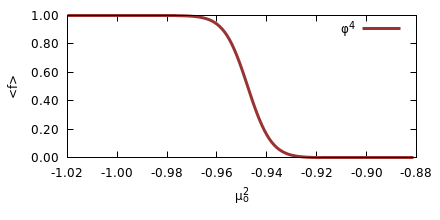
The predictive function was learned on configurations of the Ising model, but the classification knowledge can be adapted to other domains by applying it to configurations of a different system. The predictive function then becomes an observable in the target system, where multiple histogram reweighting can be employed to estimate it in the target parameter space. The results for Potts models can be seen in Fig. 2c where we recall that the phase transition is second-order for and first-order for (Baxter 1982). The dashed vertical lines indicate the positions of the analytically determined critical coupling, . Good agreement between the results obtained by transfer learning and the exact ones can already be observed on the volume shown here (). The results for the scalar field theory, a system with continuous degrees of freedom, can be seen in Fig. 2b, where we have fixed the dimensionless quartic coupling and reweighted based on the values of , the dimensionless mass parameter (see App A). We infer that the system is in the broken (ordered) phase for large and negative and in the symmetric (disordered) phase for smaller values. In Sec. IV we analyse the critical properties of the scalar field theory further using a finite-size scaling analysis.
We note that the neural network successfully differentiates between ordered and disordered phases, irrespective of the system, and despite changes in discrete or continuous degrees of freedom, the universality class and the order of the phase transition. Consequently, the predictive function learned by a convolutional neural network on the two-dimensional Ising model is capable to reconstruct effective order parameters in more complicated systems.
To gain further insights about the capability of the neural network to predict phases across different systems, we consider that the fundamental constituents of a trained neural network are the sets of variational parameters, comprised of the weights and biases at each layer of its architecture. These are optimized during the training process for a specific machine learning task . The variational parameters eventually converge to certain values which encode the solution to the particular problem under consideration. In our approach they have been tuned to accurately separate the disordered and ordered phases of the two-dimensional Ising model based on a set of labeled Ising configurations. It is well known that within the first layers of a neural network architecture the variational parameters correspond to learned universal features (Yosinski et al. 2014). This form of universality is expected to eventually diminish towards deeper layers of the neural network architecture where the features are anticipated to transition from universal to specific in relation to the machine learning task .
Considering that the 2D Ising-trained neural network successfully classifies phases across different systems by utilizing an identical predictive function , we expect universal features to extend further in deeper layers. The activation function of a variable in an intermediate layer of the neural network architecture acts as a transformation that maps a certain input to an output representation. For a feature to be deemed universal in relation to certain inputs, the corresponding activation function should produce identical output representations. We therefore present as input to the neural network configurations from different systems, and calculate their mean activations in order to diminish statistical errors during classification. The results are depicted in Fig. 3, where the activations have been drawn for the 64 variables of the first fully connected layer. We observe spikes for values of certain activations, which are consistent for configurations from the ordered or disordered phase, irrespective of the system. The features learned by the Ising-trained convolutional neural network successfully map each configuration, across systems under consideration, to its associated phase.
IV Studying unknown phase transitions
The preceding results designate that a neural network trained on a prototypical system, such as the Ising model which manifests a second-order phase transition, can serve as a tool to discover phase transitions in more complicated systems. This pursuit is greatly enhanced with the use of multiple histogram reweighting, where the entire parameter space can be examined for the discovery of a phase transition. By obtaining the knowledge of an effective order parameter through the use of transfer learning in a target system, the boundaries of its critical region can then be accurately defined.
As an example, for the field theory with fixed , we presume based on Fig. 2b, that a conservative choice for the boundaries of the ordered and disordered phases lie on values of bare mass and , respectively. We note that one could employ the neural network that produced the results of Fig. 2b to study the infinite-volume limit of the target system. However, since target systems might differ from the source system in fundamental aspects such as the order of the phase transition, the continuous degrees of freedom or the underlying symmetries, we treat the preceding results from transfer learning as qualitative indications. To obtain quantitative results, we train a randomly initialized neural network on the scalar field theory to study the infinite volume limit. We sample configurations which are labeled as belonging to each phase based on Fig. 2b. For the randomly initialized neural network, which is trained using the same setup (see App. B), the source domain is the one defined by the configurations of scalar field theory and the machine learning task is the separation of the two phases, which are discovered through transfer learning.

| 200 | -0.94988(4) | 8239(50) |
|---|---|---|
| 256 | -0.95037(5) | 12915(56) |
| 360 | -0.95096(4) | 22348(138) |
| 440 | -0.95117(3) | 34710(211) |

We proceed by performing a calculation of the critical and the critical exponents of the scalar field theory under a finite size scaling assumption, by relying on quantities derived from the neural network implementation and their reweighted extrapolations (Bachtis et al. 2020). Specifically, we associate pseudo-critical points based on the maxima of the fluctuations of the predictive function:
| (3) |
where is the volume of the system. The maxima (see Table 1) are obtained by reweighting based on one Monte Carlo dataset within the critical region. We note that including measurements from additional simulations in reweighting always leads to a reduction in statistical errors (Ferrenberg and Swendsen 1989). We then calculate the correlation length critical exponent and critical through equation:
| (4) |
and the magnetic susceptibility exponent through equation:
| (5) |
| CNN+Reweighting | -0.95225(54) | 0.99(34) | 1.78(7) |
The results are presented in Figs. 4 and 5 and in Table 2. We note that the value of the critical for fixed is within statistical errors from calculations of conventional phase transition indicators, such as the susceptibility or the Binder cumulant, in Refs. (Loinaz and Willey 1998; Schaich and Loinaz 2009). For the values of and , we anticipate the phase transition to be in the universality class of the two-dimensional Ising model, as evidenced by the calculation of the critical exponents (see App. A). In the error analysis (see App. D), only statistical errors from predictions on a finite Monte Carlo dataset were considered. Better accuracy can be achieved by including calculations from additional lattice sizes.
V Conclusions
In this paper we employed transfer learning to discover and study phase transitions from ordered to disordered phases in two-dimensional statistical systems. By employing an Ising-trained convolutional neural network and multi-histogram reweighting, we reconstructed effective order parameters in q-state Potts models and the scalar field theory, without introducing prior knowledge about the presence of a phase transition in those target systems. In addition we viewed the neural network as a mapping that associates each configuration, across different systems, to its corresponding phase and uncovered universal features learned on deeper layers of the neural network architecture. Furthermore we utilized transfer learning to define the boundaries of the critical region in the scalar field theory. We finally conducted a finite size scaling analysis to calculate multiple critical exponents and the critical constant using quantities derived solely from the neural network algorithm. We are not aware of any prior work that employs machine learning to calculate critical exponents for a quantum field theory.
The discovery and study of an unknown phase transition can be completed in four steps:
- •
A neural network is trained on labeled configurations of an original system to learn a predictive function that separates a number of phases.
- •
The predictive function is then applied on unlabeled configurations of a target system, to recognize if they belong to any of the learned phases. The entire parameter space can be inspected with multiple histogram reweighting to uncover the target system’s critical region.
- •
Given this knowledge a second neural network is trained on configurations of the target system that have been labelled in compliance with the recognized phases in the previous step.
- •
The infinite volume limit is studied, using reweighting on derived quantities from the second neural network implementation to determine the universality class of the phase transition in the target system.
Transfer learning enables the use of simplistic systems to study complicated models with partially known behaviour. Combined with multi-histogram reweighting, a technique that is able to scan the entire parameter space by reconstructing effective order parameters therein, it permits the discovery of unknown phase transitions. Transfer learning is employed successfully to predict the phase structure of target systems irrespective of the universality class, order, and discrete or continuous degrees of freedom, and can therefore be employed to uncover phase transitions in seemingly unrelated systems. Finally one could combine multiple transfer learning implementations, obtained by training neural networks on models with different phase transitions, to predict the structure of an intricate, unknown phase transition in a target system.
Note added: During completion of this manuscript, Refs. (Yau and Su 2020; Mendes-Santos et al. 2020) appeared on the arXiv. Ref. (Yau and Su 2020) employs transfer learning for Potts models, and Ref. (Mendes-Santos et al. 2020) explores universal critical behaviour of phase transitions based on the intrinsic dimension in the data space.
VI Acknowledgements
The authors received funding from the European Research Council (ERC) under the European Union’s Horizon 2020 research and innovation programme under grant agreement No 813942. The work of GA and BL has been supported in part by the STFC Consolidated Grant ST/P00055X/1. The work of BL is further supported in part by the Royal Society Wolfson Research Merit Award WM170010. Numerical simulations have been performed on the Swansea SUNBIRD system. This system is part of the Supercomputing Wales project, which is part-funded by the European Regional Development Fund (ERDF) via Welsh Government. We thank COST Action CA15213 THOR for support.
Appendix A Ising, Potts and the field theory
We consider the q-state Potts model on a square lattice, with a Hamiltonian:
| (6) |
where denotes the coupling constant, which we set to one, is a sum over nearest neighbour interactions, is the Kronecker delta and is a spin at lattice site that can take the values . The 2D Potts model has a second-order phase transition for and a first-order phase transition for (Baxter 1982). For , , , the Potts model reduces to the Ising model. The inverse critical temperature of the 2D q-state Potts model is given by:
| (7) |
where for , .
We consider the scalar field theory in two dimensions, described by the Euclidean Lagrangian:
| (8) |
We discretize the scalar field theory on a square lattice with lattice spacing :
where the dimensionless parameters and are the (bare) mass squared and coupling constant. By fixing the value of while varying we cross a second-order phase transition in the plane (Loinaz and Willey 1998). When and the system is expected to be in the same universality class as the 2D Ising model, whereas for fixed and the emerging critical behaviour is Gaussian (Milchev et al. 1986).
Appendix B Convolutional Neural Network
The neural network architecture, implemented with TensorFlow and the Keras library, is comprised of a convolutional layer with 64 filters, of size and a stride of . The result is then forwarded to a max-pooling layer of size and subsequently to a fully-connected layer (FC1) with 64 latent variables. The non-linear function is chosen as a rectified linear unit . The output layer consists of a fully connected layer (FC2) with a softmax activation function and the training is conducted with the Adam algorithm and a mini batch size of 12. The architecture was optimized for the Ising model based on the training and validation loss.
The neural network is trained on 1000 uncorrelated configurations per each parameter choice. Specifically for the case of the Ising model the range of inverse temperatures is and in the disordered and the ordered phase respectively, with a step size of . The second neural network is trained independently on the field theory on values of bare mass and with the same step size.
Appendix C Multi-Histogram Reweighting
During a Monte Carlo simulation the probability of generating a state with a lattice action (or energy) is:
| (9) |
where the density of states, the partition function and a lattice action (or Hamiltonian) that separates in terms of a set of parameters :
| (10) |
The probability can be estimated during a Monte Carlo simulation through where is the number of independent measurements and the histograms of the action. After conducting a series of simulations for a specific set of parameters , we arrive at a number of different estimates of the density of states, given by:
| (11) |
The estimates can be combined through a weighted average to estimate the density of states :
| (12) |
The values are acquired through a minimization of the variance in the density of states, resulting in the equation:
| (13) |
where is the number of available Monte Carlo datasets. For each dataset, simulated on a parameter set , the partition function, given by equation:
| (14) |
can be estimated through an iterative scheme (Ferrenberg and Swendsen 1989; Newman and Barkema 1999), by solving:
| (15) |

After convergence, the partition function for an interpolated parameter set can be acquired by one iteration of Eq. 15. The expectation value of an arbitrary observable for a set of parameters is then calculated using equation:
| (16) |
where is the number of states sampled at simulation. By carefully conducting simulations in order to obtain overlapping histograms between parameter values (e.g. see Fig. 6) one can calculate the partition function and arbitrary observables of interest in the entire parameter space using Eqs. 15 and 16.
Appendix D Binning Error Analysis
The error analysis is conducted with a binning approach. A Monte Carlo dataset, comprised of 10000 uncorrelated measurements, is separated into groups of 1000 measurements. Multi-histogram reweighting is conducted times for extrapolated sets of parameters using the measurements of each group in each available simulation. The standard deviation for the expectation value at each extrapolated parameter is given through equation:
| (17) |
References
- Goodfellow et al. (2016) I. J. Goodfellow, Y. Bengio, and A. Courville, Deep Learning (MIT Press, Cambridge, MA, USA, 2016) http://www.deeplearningbook.org.
- Carleo et al. (2019) G. Carleo, I. Cirac, K. Cranmer, L. Daudet, M. Schuld, N. Tishby, L. Vogt-Maranto, and L. Zdeborová, Machine learning and the physical sciences, Reviews of Modern Physics 91, 10.1103/revmodphys.91.045002 (2019).
- Carrasquilla and Melko (2017) J. Carrasquilla and R. G. Melko, Machine learning phases of matter, Nature Physics 13, 431 (2017).
- van Nieuwenburg et al. (2017) E. L. van Nieuwenburg, Y.-H. Liu, and S. Huber, Learning phase transitions by confusion, Nature Physics 13, 435 (2017).
- Broecker et al. (2017) P. Broecker, J. Carrasquilla, R. G. Melko, and S. Trebst, Machine learning quantum phases of matter beyond the fermion sign problem, Scientific Reports 7, 8823 (2017).
- Ch’ng et al. (2017) K. Ch’ng, J. Carrasquilla, R. G. Melko, and E. Khatami, Machine learning phases of strongly correlated fermions, Phys. Rev. X 7, 031038 (2017).
- Tanaka and Tomiya (2017) A. Tanaka and A. Tomiya, Detection of phase transition via convolutional neural networks, Journal of the Physical Society of Japan 86, 063001 (2017), https://doi.org/10.7566/JPSJ.86.063001 .
- Torlai and Melko (2016) G. Torlai and R. G. Melko, Learning thermodynamics with boltzmann machines, Phys. Rev. B 94, 165134 (2016).
- Suchsland and Wessel (2018) P. Suchsland and S. Wessel, Parameter diagnostics of phases and phase transition learning by neural networks, Phys. Rev. B 97, 174435 (2018).
- Ni et al. (2019) Q. Ni, M. Tang, Y. Liu, and Y.-C. Lai, Machine learning dynamical phase transitions in complex networks, Phys. Rev. E 100, 052312 (2019).
- Hsu et al. (2018) Y.-T. Hsu, X. Li, D.-L. Deng, and S. Das Sarma, Machine learning many-body localization: Search for the elusive nonergodic metal, Phys. Rev. Lett. 121, 245701 (2018).
- van Nieuwenburg et al. (2018) E. van Nieuwenburg, E. Bairey, and G. Refael, Learning phase transitions from dynamics, Phys. Rev. B 98, 060301 (2018).
- Venderley et al. (2018) J. Venderley, V. Khemani, and E.-A. Kim, Machine learning out-of-equilibrium phases of matter, Phys. Rev. Lett. 120, 257204 (2018).
- Alexandrou et al. (2019) C. Alexandrou, A. Athenodorou, C. Chrysostomou, and S. Paul, Unsupervised identification of the phase transition on the 2d-ising model (2019), arXiv:1903.03506 [cond-mat.stat-mech] .
- Chernodub et al. (2020) M. N. Chernodub, H. Erbin, V. A. Goy, and A. V. Molochkov, Topological defects and confinement with machine learning: The case of monopoles in compact electrodynamics, Phys. Rev. D 102, 054501 (2020).
- Zhou et al. (2019) K. Zhou, G. Endrődi, L.-G. Pang, and H. Stöcker, Regressive and generative neural networks for scalar field theory, Phys. Rev. D 100, 011501 (2019).
- Nicoli et al. (2020) K. A. Nicoli, S. Nakajima, N. Strodthoff, W. Samek, K.-R. Müller, and P. Kessel, Asymptotically unbiased estimation of physical observables with neural samplers, Phys. Rev. E 101, 023304 (2020).
- Rodriguez-Nieva and Scheurer (2019) J. F. Rodriguez-Nieva and M. S. Scheurer, Identifying topological order through unsupervised machine learning, Nature Physics 15, 790 (2019).
- Ponte and Melko (2017) P. Ponte and R. G. Melko, Kernel methods for interpretable machine learning of order parameters, Phys. Rev. B 96, 205146 (2017).
- Giannetti et al. (2019) C. Giannetti, B. Lucini, and D. Vadacchino, Machine learning as a universal tool for quantitative investigations of phase transitions, Nuclear Physics B 944, 114639 (2019).
- Greitemann et al. (2019) J. Greitemann, K. Liu, and L. Pollet, Probing hidden spin order with interpretable machine learning, Phys. Rev. B 99, 060404 (2019).
- Liu et al. (2019) K. Liu, J. Greitemann, and L. Pollet, Learning multiple order parameters with interpretable machines, Phys. Rev. B 99, 104410 (2019).
- Wang (2016) L. Wang, Discovering phase transitions with unsupervised learning, Phys. Rev. B 94, 195105 (2016).
- Hu et al. (2017) W. Hu, R. R. P. Singh, and R. T. Scalettar, Discovering phases, phase transitions, and crossovers through unsupervised machine learning: A critical examination, Phys. Rev. E 95, 062122 (2017).
- Wang and Zhai (2017) C. Wang and H. Zhai, Machine learning of frustrated classical spin models. i. principal component analysis, Phys. Rev. B 96, 144432 (2017).
- Costa et al. (2017) N. C. Costa, W. Hu, Z. J. Bai, R. T. Scalettar, and R. R. P. Singh, Principal component analysis for fermionic critical points, Phys. Rev. B 96, 195138 (2017).
- Zhang et al. (2019) W. Zhang, L. Wang, and Z. Wang, Interpretable machine learning study of the many-body localization transition in disordered quantum ising spin chains, Phys. Rev. B 99, 054208 (2019).
- Canabarro et al. (2019) A. Canabarro, F. F. Fanchini, A. L. Malvezzi, R. Pereira, and R. Chaves, Unveiling phase transitions with machine learning, Phys. Rev. B 100, 045129 (2019).
- Shiina et al. (2020) K. Shiina, H. Mori, Y. Okabe, and H. K. Lee, Machine-learning studies on spin models, Scientific Reports 10, 2177 (2020).
- Zen et al. (2020) R. Zen, L. My, R. Tan, F. Hébert, M. Gattobigio, C. Miniatura, D. Poletti, and S. Bressan, Transfer learning for scalability of neural-network quantum states, Phys. Rev. E 101, 053301 (2020).
- Carleo and Troyer (2017) G. Carleo and M. Troyer, Solving the quantum many-body problem with artificial neural networks, Science 355, 602–606 (2017).
- Huembeli et al. (2018) P. Huembeli, A. Dauphin, and P. Wittek, Identifying quantum phase transitions with adversarial neural networks, Phys. Rev. B 97, 134109 (2018).
- Pan and Yang (2010) S. J. Pan and Q. Yang, A survey on transfer learning, IEEE Trans. on Knowl. and Data Eng. 22, 1345–1359 (2010).
- Bachtis et al. (2020) D. Bachtis, G. Aarts, and B. Lucini, Extending machine learning classification capabilities with histogram reweighting, Phys. Rev. E 102, 033303 (2020).
- Ferrenberg and Swendsen (1989) A. M. Ferrenberg and R. H. Swendsen, Optimized monte carlo data analysis, Phys. Rev. Lett. 63, 1195 (1989).
- Ferrenberg and Swendsen (1988) A. M. Ferrenberg and R. H. Swendsen, New monte carlo technique for studying phase transitions, Phys. Rev. Lett. 61, 2635 (1988).
- Wolff (1989) U. Wolff, Collective monte carlo updating for spin systems, Phys. Rev. Lett. 62, 361 (1989).
- Loinaz and Willey (1998) W. Loinaz and R. S. Willey, Monte carlo simulation calculation of the critical coupling constant for two-dimensional continuum theory, Phys. Rev. D 58, 076003 (1998).
- Brower and Tamayo (1989) R. C. Brower and P. Tamayo, Embedded dynamics for theory, Phys. Rev. Lett. 62, 1087 (1989).
- Baxter (1982) R. Baxter, Exactly solved models in statistical mechanics (1982).
- Yosinski et al. (2014) J. Yosinski, J. Clune, Y. Bengio, and H. Lipson, How transferable are features in deep neural networks?, in Advances in Neural Information Processing Systems 27, edited by Z. Ghahramani, M. Welling, C. Cortes, N. D. Lawrence, and K. Q. Weinberger (Curran Associates, Inc., 2014) pp. 3320–3328.
- Schaich and Loinaz (2009) D. Schaich and W. Loinaz, Improved lattice measurement of the critical coupling in theory, Phys. Rev. D 79, 056008 (2009).
- Yau and Su (2020) H. M. Yau and N. Su, On the generalizability of artificial neural networks in spin models (2020), arXiv:2006.15021 [cond-mat.dis-nn] .
- Mendes-Santos et al. (2020) T. Mendes-Santos, X. Turkeshi, M. Dalmonte, and A. Rodriguez, Unsupervised learning universal critical behavior via the intrinsic dimension (2020), arXiv:2006.12953 [cond-mat.stat-mech] .
- Milchev et al. (1986) A. Milchev, D. W. Heermann, and K. Binder, Finite-size scaling analysis of the 4 field theory on the square lattice, Journal of Statistical Physics 44, 749 (1986).
- Newman and Barkema (1999) M. E. J. Newman and G. T. Barkema, Monte Carlo methods in statistical physics (Clarendon Press, Oxford, 1999).