Non-Homogeneous Poisson Process Intensity Modeling and Estimation using Measure Transport

Consider two probability measures $\mu_{0}(\cdot)$ and $\mu_{1}(\cdot)$ defined on ${\cal X}$ and ${\cal Z}$, respectively. A transport map $T:{\cal X}\rightarrow{\cal Z}$ is said to push forward $\mu_{0}(\cdot)$ to $\mu_{1}(\cdot)$ (written compactly as $T_{\#\mu_{0}}(\cdot)=\mu_{1}(\cdot)$) if and only if

The inverse $T^{-1}(\cdot)$ is treated in the general set valued sense, that is, $x\in T^{-1}(z)$ if $T(x)=z$. If $T(\cdot)$ is injective, then the relationship in (1) can also be expressed as

A transport map satisfying (1) represents a deterministic coupling of the probability measures $\mu_{0}(\cdot)$ and $\mu_{1}(\cdot)$. An alternative interpretation of the transport map $T(\cdot)$ is that if $v$ is a random vector distributed according to the measure $\mu_{0}(\cdot)$, then $T(v)$ is distributed according to $\mu_{1}(\cdot)$.

Suppose ${\cal X},{\cal Z}\subseteq\mathbb{R}^{d}$, and that both $\mu_{0}(\cdot)$ and $\mu_{1}(\cdot)$ are absolutely continuous with respect to the Lebesgue measure on $\mathbb{R}^{d}$, with densities $\mbox{d}\mu_{0}(x)=f_{0}(x)\mbox{d}x$ and $\mbox{d}\mu_{1}(z)=f_{1}(z)\mbox{d}z$, respectively. Furthermore, assume that the map $T(\cdot)$ is bijective differentiable with a differentiable inverse $T^{-1}(\cdot)$ (i.e., assume that $T(\cdot)$ is a $C^{1}$ diffeomorphism), then (2) is equivalent to

Various approaches to parameterize an increasing triangular map have been proposed (Germain et al., 2015; Dinh et al., 2015; Dinh et al., 2017, see, for example, ). One class of parameterizations is based on the so-called “conditional networks” (Papamakarios et al., 2017; Huang et al., 2018). Consider for now a map comprising just one increasing triangular map, which we denote as $T_{1}(\cdot)$ (we will later consider many of these in composition), and let $x\equiv(x^{(1)},\ldots,x^{(d)})^{\prime}$. The increasing triangular map $T_{1}(\cdot)$ we use has the following form:

for $x\in{\cal X}$, where $\theta_{1k}(x^{(1)},\ldots,x^{(k-1)};\vartheta_{1k}),k=2,\dots,d,$ is the $k$th “conditional network” that takes $x^{(1)},\ldots,x^{(k-1)}$ as inputs and is parameterized by $\vartheta_{1k}$, and $S_{1}^{(k)}(\cdot)$ is generally a very simple univariate function of $x^{(k)}$, but with parameters that depend in a relatively complex manner on $x^{(1)},\ldots,x^{(k-1)}$ through the network. Therefore, a conditional network is just a multivariate mapping that takes input $x^{(1)},\ldots,x^{(k-1)}$ and returns an output in $\mathbb{R}^{m_{k}}$, where $m_{k}$ is the number of parameters that parameterize $S_{1}^{(k)}(\cdot)$. We hence have that $\theta_{1k}:\mathbb{R}^{k-1}\rightarrow\mathbb{R}^{m_{k}}$. It is often the case that feedforward neural networks are used as the conditional networks (Fine et al., 1999). For ease of exposition, from now on we will slightly abuse the notation and denote $\theta_{1k}(x^{(1)},\ldots,x^{(k-1)};\vartheta_{1k})$ simply as $\theta_{1k}$, thereby omitting the explicit dependence on the inputs and the parameters $\vartheta_{1k}$.

One class of maps using conditional networks is that of masked autoregressive flows (Papamakarios et al., 2017). In this class, $m_{k}=2,~k=1,\dots,d$, and the output of the conditional network $\theta_{1k}\equiv(\theta_{1k}^{(1)},\theta_{1k}^{(2)})^{\prime}\in\mathbb{R}^{2}$ parameterizes $S_{1}^{(k)}(\cdot)$ as

In (6), the univariate function $S_{1}^{(k)}(\cdot)$ is a linear function of $x^{(k)}$ with location parameter $\theta_{1k}^{(1)}$ and scale parameter $\exp(\theta_{1k}^{(2)})$. Monotonicity of $S_{1}^{(k)}(\cdot)$, and hence of $T_{1}^{(k)}(\cdot)$, is ensured since $\exp(\theta_{1k}^{(2)})>0$. Another class of such maps is the class of inverse autoregressive flows, proposed by Kingma et al., 2016. In this class, $m_{k}=2,k=1,\dots,d,$ and

where $\sigma(\cdot)$ is the sigmoid function. In this class of maps, each $S_{1}^{(k)}(x^{(k)})$ outputs the weighted average of $x^{(k)}$ and $\theta_{1k}^{(1)}$, with the weights given by $\sigma(\theta_{1k}^{(2)})$ and $1-\sigma(\theta_{1k}^{(2)})$, respectively. Monotonicity of $S_{1}^{(k)}(\cdot)$, and hence of $T_{1}^{(k)}(\cdot)$, is ensured since $\sigma(\theta_{1k}^{(2)})>0$.

Both (6) and (7) are generally too simple for modeling density functions or, in our case, intensity functions. In this work we therefore focus on the class of neural autoregressive flows, proposed by Huang et al., 2018, which are more flexible. In this class, $m_{k}=3M$ for $k=1,\dots,d,$ and $M\geq 1$, and the $k$-th component of the map has the form

where $\sigma^{-1}(\cdot)$ is the logit function, $a_{1ki}\equiv\exp(\theta_{1k}^{(2i)})$, $b_{1ki}\equiv\theta_{1k}^{(3i)}$, and $w_{1ki}\equiv\exp(\theta_{1k}^{(1i)})$ is subject to the constraint $\sum_{i=1}^{M}w_{1ki}=1$. As with the other two maps discussed above, monotonicity of $S_{1}^{(k)}(\cdot)$, and hence of $T_{1}^{(k)}(\cdot)$, is ensured through this construction. The Jacobian of the neural autoregressive flow can be computed using the chain rule since the gradient of both $\sigma(\cdot)$ and $\sigma^{-1}(\cdot)$ are analytically available; this is important for computational purposes since such formulations can easily be handled using automatic differentiation libraries.

Each univariate function $S_{1}^{(k)}(\cdot)$ in the neural autoregressive flow comprises two sets of smooth, nonlinear transforms: $M$ sigmoid functions that map from $\mathbb{R}$ to the unit interval, and one logit function that maps from the unit interval to $\mathbb{R}$. The complexity/flexibility of $S_{1}^{(k)}(\cdot)$ is largely determined by $M$. Note that the neural autoregressive flow has a very similar form to the conventional feedforward neural network with sigmoid activation functions.

It is straightforward to see that each component of the increasing triangular map constructed above is differentiable. Indeed, $S_{1}^{(k)}(x^{(k)};\theta_{1k})$ in (8) is obviously differentiable with respect to $x^{(k)}$. Also, $S_{1}^{(k)}(x^{(k)};\theta_{1k})$, when treated as a function of $\theta_{1k}$, is clearly differentiable with respect to $\theta_{1k}$, while the conditional network $\theta_{1k}(x^{(1)},\ldots,x^{(k-1)};\vartheta_{1k})$ is also differentiable with respect to the input $x^{(1)},\ldots,x^{(k-1)}$ if it itself is a feedforward neural network with sigmoid activation functions, which we will assume from now on. Therefore, $T_{1}^{(k)}(x^{(1)},\ldots,x^{(k)})=S_{1}^{(k)}(x^{(k)};\theta_{1k}(x^{(1)},\ldots,x^{(k-1)};\vartheta_{1k}))$ is also differentiable with respect to $x^{(1)},\ldots,x^{(k-1)}$ for $k=1,\dots,d$.

A natural question to ask is how well an arbitrary density function can be approximated by a density constructed using the neural autoregressive flow. It has been shown that the neural autoregressive flow satisfies the ‘universal property’ for the set of positive continuous probability density functions, in the sense that any target density that satisfies mild smoothness assumptions can be approximated arbitrarily well (Huang et al., 2018). We provide a universal approximation theorem for the case of the process density of a Poisson process in Section 3.3.

It is well known that a neural network with one hidden layer can be used to approximate any continuous function on a bounded domain arbitrarily well (Hornik et al., 1989; Cybenko, 1989; Barron, 1994). However, the size of a single layer network (in terms of the number of parameters) that may be required to achieve a desired level of function approximation accuracy may be prohibitively large. This is important as, despite the universal property of the neural autoregressive flow, both the conditional network and the univariate function $S_{1}^{(k)}(\cdot)$ in (8) may need to be made very complex in order to approximate a target density up to a desired level of accuracy. Specifically, $M$, as well as the number of parameters appearing in the conditional networks, $\{\vartheta_{1k}\}$, might be prohibitively large.

Neural networks with many hidden layers, known as deep nets, tend to have faster convergence rates to the target function compared to shallow networks (Eldan and Shamir, 2016; Weinan and Wang, 2018). In our case, layering several relatively parsimonious triangular maps through composition is an attractive way of achieving the required representational ability while avoiding an explosion in the number of parameters. Specifically, we let $T(\cdot)=T_{N}\circ\cdots\circ T_{1}(\cdot)$, where $T_{l}(\cdot),l=1,\dots,N$, are increasing triangular maps of the form given in (2.2), parameterized using neural autoregressive flows.

The composition does not break the required bijectivity of $T(\cdot)$, since a bijective function of a bijective function is itself bijective. Computations also remain tractable, since the determinant of the gradient of the composition is simply the product of the determinants of the individual gradients. Specifically, consider two increasing triangular maps $T_{1}(\cdot)$ and $T_{2}(\cdot)$, each constructed using the neural network approach described above. The composition $T_{2}\circ T_{1}(\cdot)$ is bijective, and its gradient at some $x\in\cal X$ has determinant,

Further, since the maps have a triangular structure, the Jacobian at some point $x$ is a triangular matrix, for which the determinant is easy to compute. The determinant of the composition evaluated at $x$ is hence also easy to compute.

The density of a Poisson process does not exist with respect to the Lebesgue measure. It is therefore customary to instead consider the density of the NHPP of interest with respect to the density of the unit rate Poisson process, that is, the process with $\lambda(\cdot)=1$. We denote the resulting density as $f_{\lambda}(\cdot)$. Let $|B|$ denote the Lebesgue measure of a bounded set $B\subset\mathbb{R}^{d}$, and let $X\equiv\{x_{1},\ldots,x_{n}\},$ where $x_{i}\in{\cal X},i=1,\ldots,n,$ and $n\geq 1,$ be a realization of ${\cal P}$. The density function $f_{\lambda}(\cdot)$ evaluated at $X$ is given by,

Using the process-density representation of the intensity function, and the Monte Carlo approximations (12) and (13), we re-express the optimization problem (10) in terms of the estimate of the integrated intensity, $\hat{\mu}_{\lambda}({\cal X})$, and the estimated process density $\hat{\tilde{\lambda}}(\cdot)$,

where now $\tilde{\cal A}$ is some set of process densities, which we will establish in Section 3.2. It is easy to see that setting $\mu_{\rho}({\cal X})=n$ minimizes the objective function in (14). Fixing $\mu_{\rho}({\cal X})=n$ leads us to the optimization problem

which is equivalent to maximizing the likelihood of observing $X$.

We model the process density $\tilde{\rho}(\cdot)$ using the transportation of probability measure approach described in Section 2. Specifically, we seek a diffeomorphism $T:{\cal X}\rightarrow{\cal Z}$, where ${\cal Z}$ need not be the same as ${\cal X}$, such that

where $\eta(\cdot)$ is some simple reference density on ${\cal Z}$, and $|\mbox{det}\nabla T(\cdot)|>0$. Popular choices of $\eta(\cdot)$ include the standard normal distribution if ${\cal Z}$ is unbounded, and the uniform distribution if ${\cal Z}$ is bounded.

While the domain and the range of the map $T(\cdot)$ can be arbitrary subsets of $\mathbb{R}^{d}$, it is generally easier to construct transport maps from $\mathbb{R}^{d}$ to $\mathbb{R}^{d}$. The domain $\cal X$ is bounded, and therefore we can assume, without loss of generality, that ${\cal X}=(0,1)^{d}$, and we first apply an element-wise logit transform to each coordinate of the vector $x=(x^{(1)},\ldots,x^{(d)})^{{}^{\prime}}$ to obtain the vector $y\equiv(y^{(1)},\dots,y^{(d)})^{\prime}\in\mathbb{R}^{d}$, where $y^{(k)}=\sigma^{-1}(x^{(k)}),\quad k=1,\ldots,d$. The Jacobian of this transformation is given by $\prod_{k=1}^{d}((x^{(k)})^{-1}+(1-x^{(k)})^{-1})$. We subsequently construct the transport map $T(\cdot)$ as a composition of $N$ increasing triangular maps $T_{N}\circ T_{N-1}\circ\,\cdots\,\circ T_{1}(\cdot)$ (see Section 2.3). Each triangular map $T_{j}(\cdot),j=1,\ldots,N,$ in the composition is parameterized using a conditional network approach as detailed in Section 2.2. Specifically, we adopt the neural autoregressive flow where the $k$th component of each triangular map is modeled as in (8).

Denote the parameters appearing in the $k$th conditional network associated with the $j$th layer as $\vartheta_{jk}$ and let $\boldsymbol{\Theta}\equiv\{\theta_{j1}:j=1,\dots,N\}\cup\{\vartheta_{jk}:k=2,\dots,d;j=1,\dots,N\}$. The optimization problem (15) reduces to the optimization problem:

The optimization problem can be solved efficiently using automatic differentiation libraries, stochastic gradient descent, and graphics processing units for efficient computation. We used PyTorch for our implementation (Paszke et al., 2017) and adapted the code provided by Huang et al., 2018.

The increasing triangular maps constructed using neural autoregressive flows (8) satisfy a universal property in the context of probability density approximation. This universal approximation property naturally applies to the process density of a Poisson process. One need only prove this property for the case of one triangular map since, if two maps have the universal property, their composition also has the universal property.

1. 1.

   We first establish in Lemma A.1 in Appendix A.2 that any process density $\tilde{\lambda}(\cdot)$ that satisfies the conditions in Theorem 3.1 can be expressed as $\tilde{\lambda}(\cdot)=\eta(\tilde{T}(\cdot))\mbox{det}(\nabla\tilde{T}(\cdot))$, where $\tilde{T}(\cdot)$ is some increasing continuous differentiable triangular map.
   

2. 2.

   Lemmas A.2 and A.3 in Appendix A.2 establish that, for any increasing continuously differentiable triangular map $\tilde{T}(\cdot)$ and for any $\epsilon>0$,

   $$|\tilde{T}^{(k)}(x^{(1)},\ldots,x^{(k)})-S^{(k)}(x^{(k)};\tilde{\theta}_{k}(x^{(1)},\ldots,x^{(k-1)}))|<\epsilon/2,$$

   $$|\nabla_{k}\tilde{T}^{(k)}(x^{(1)},\ldots,x^{(k)})-\nabla S^{(k)}(x^{(k)};\tilde{\theta}_{k}(x^{(1)},\ldots,x^{(k-1)}))|<\epsilon/2,$$

   for $k=2,\ldots,d$, where $\nabla_{k}$ denotes the derivative with respect to the $k$-th component of the input, and $\tilde{\theta}_{k}(\cdot)$ is some arbitrary continuous mapping from $(x^{(1)},\ldots,x^{(k-1)})$ to the set of parameters $a_{ki},b_{ki},w_{ki},i=1,\dots,M$.
   

3. 3.

   By the universality of feedforward neural networks with sigmoid activation functions, and uniform continuity of $S^{(k)}(\cdot)$ and $\nabla S^{(k)}(\cdot)$, we have that

   $$|S^{(k)}(x^{(k)};\tilde{\theta}_{k}(x^{(1)},\ldots,x^{(k-1)}))-S^{(k)}(x^{(k)};\hat{\theta}_{k}(x^{(1)},\ldots,x^{(k-1)}))|<\epsilon/2,$$

   $$|\nabla S^{(k)}(x^{(k)};\tilde{\theta}_{k}(x^{(1)},\ldots,x^{(k-1)}))-\nabla S^{(k)}(x^{(k)};\hat{\theta}_{k}(x^{(1)},\ldots,x^{(k-1)}))|<\epsilon/2,$$

   for $k=2,\ldots,d$, where $\hat{\theta}_{k}(\cdot)$ is a feedforward neural network with sigmoid activation functions.
   

4. 4.

   An application of the triangle inequality yields

   $$|\tilde{T}^{(k)}(x^{(1)},\ldots,x^{(k)})-S^{(k)}(x^{(k)};\hat{\theta}^{(k)}(x^{(1)},\ldots,x^{(k-1)}))|<\epsilon,$$

   $$|\nabla_{k}\tilde{T}^{(k)}(x^{(1)},\ldots,x^{(k)})-\nabla S^{(k)}(x^{(k)};\hat{\theta}_{k}(x^{(1)},\ldots,x^{(k-1)}))|<\epsilon,$$

   for $k=2,\ldots,d$. Therefore, for an arbitrary increasing continuous differentiable triangular map $\tilde{T}(\cdot)$, there exists a triangular map $T(\cdot)$ where the $k$-th component of $T(\cdot)$ is $S^{(k)}(x^{(k)};\hat{\theta}_{k}(x^{(1)},\ldots,x^{(k-1)}))$ such that

   $$|T^{(k)}(x^{(1)},\ldots,x^{(k)})-\tilde{T}^{(k)}(x^{(1)},\ldots,x^{(k)})|<\epsilon,$$

   $$|\nabla_{k}T^{(k)}(x^{(1)},\ldots,x^{(k)})-\nabla_{k}\tilde{T}^{(k)}(x^{(1)},\ldots,x^{(k)})|<\epsilon,$$

   for $k=2,\ldots,d$. We naturally also have that

   $$|T^{(1)}(x^{(1)})-\tilde{T}^{(1)}(x^{(1)})|<\epsilon,$$

   $$|\nabla_{1}T^{(1)}(x^{(1)})-\nabla_{1}\tilde{T}^{(1)}(x^{(1)})|<\epsilon,$$

   where $T^{(1)}(x^{(1)})=S^{(1)}(x^{(1)};\hat{\theta}_{1})$.
   

5. 5.

   Finally, since $\mbox{det}(\nabla T(x))=\prod_{k=1}^{d}\nabla_{k}T^{(k)}(x)$, and the target density $\eta(\cdot)$ is smooth, both $|\mbox{det}(\nabla T(x))-\mbox{det}(\nabla\tilde{T}(x))|$, and $|\eta(T(x))-\eta(\tilde{T}(x))|,$ can be made arbitrarily small for all $x\in\mathcal{X}$. This implies that

   $$|\eta(T(x))\mbox{det}(\nabla T(x))-\eta(\tilde{T}(x))\mbox{det}(\nabla\tilde{T}(x))|,$$

   can be made arbitrarily small for all $x\in\mathcal{X}$, which completes the proof.

An attraction of using measure transport is that one can readily simulate data based on the estimated intensity function without resorting to methods like thinning, which can be inefficient when the Poisson process is highly non-homogeneous. Here, one simulates from the simple, known reference density $\eta(\cdot)$, and then pushes back the points through the inverse map. Since the maps we use are triangular, their inverse can be found in a relatively straightforward manner.

Consider a point $z=(z^{(1)},\ldots,z^{(d)})^{{}^{\prime}}$ in the reference domain. We give an algorithm for computing $T^{-1}(z)$, where $T(\cdot)$ is a (single) increasing triangular map, in Algorithm 1. Note that inversion under the increasing triangular map involves solving $d$ univariate root-finding problems. These problems can be efficiently solved since each component of the map is continuous and increasing.

Now, when we have $N$ triangular maps in composition, $T_{N}\circ T_{N-1}\circ\cdots\circ T_{1}(\cdot)$ say, we can compute the inverse by iteratively applying Algorithm 1 using $T_{N}(\cdot),T_{N-1}(\cdot),\ldots,T_{1}(\cdot)$. Algorithm 2 gives an algorithm for simulating from the fitted point process for the case when the reference probability measure is the standard multivariate normal distribution.

The intensity function is fitted by solving the problem given in (16). The standard error of the fitted intensity function can be estimated using a non-parametric bootstrapping approach (Efron, 1981). We construct $B$ bootstrap samples by drawing the number of points $n_{b},b=1,\dots,B$, from a Poisson distribution with rate parameter $n$. For each $b=1,\dots,B$ we then randomly sample $n_{b}$ points from the observed points $X$ with replacement, and fit the process density to each of these bootstrap samples, to obtain $B$ estimated process densities $\hat{\tilde{\lambda_{b}}}(\cdot),b=1,\dots,B$. The standard error of the intensity function evaluated at any point $x\in{\cal X}$ is then obtained by finding the empirical standard deviation of $\{n_{b}\hat{\tilde{\lambda}}_{b}(x):b=1,\dots,B\}$. Algorithm 3 gives a summary.

Standard error estimation can also be performed using a parametric bootstrap approach (Efron, 1979), where bootstrap samples are obtained from the fitted intensity function. However, this would require running Algorithms 1 and 2 $B$ times, which would be considerably more computationally demanding. We therefore do not consider this bootstrap strategy here.

In this section we illustrate our method on simulated data in both a one dimensional and a two dimensional setting. Our method requires one to specify the number of compositions of triangular maps, the width of the neural network in the triangular maps, the number of layers in the conditional networks (feedforward neural networks), and the width of each layer in each conditional network. In neural networks and deep learning literature, choosing the optimal network structure is an open problem. For shallow feedforward neural networks, that is, neural networks with one or two hidden layers, information criteria based methods (Fogel, 1991) and heuristic algorithms (Leung et al., 2003; Jinn-Tsong Tsai et al., 2006) have been proposed to determine the optimal width of the network. However, to the best of our knowledge, analogous methods are not available for deep neural networks and neural networks with complicated structure. In higher dimensional problems, there is theoretical support for adopting a very deep neural network structure due to its representational power (Eldan and Shamir, 2016; Raghu et al., 2017). However, since point process realizations typically lie in lower dimensional space, such results are less relevant.

We found that in low-dimensional settings our estimates did not change considerably with the number of layers in the conditional network and therefore, here, we fix the number of layers to one. That is, we let each $\theta_{jk}^{(i)}(\cdot)$ be the output of a neural network of one layer. In both simulation experiments we set the widths of the neural networks in both the triangular maps (i.e., $M$) and the conditional networks, to 64. We set this number by successively increasing the network widths in powers of two until the intensity-function estimate was not improved. We also used network widths of 64 in the application case study of Section 4.2. The learning rate for the optimization is set to $10^{-4}$ in all our experiments.

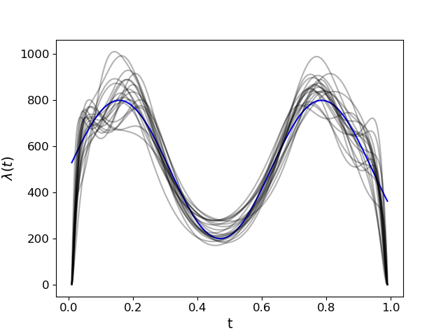
For the one dimensional studies, we first simulated events (via thinning) from the following two one-dimensional intensity functions,

We then fitted several models to the simulated events, each with a different number of compositions of triangular maps. The procedure of simulating and model fitting was repeated 40 times in order to assess the variability in the estimated intensity functions. Each model fitting required approximately two minutes on a graphics processing unit.

The average and empirical standard deviation of the $L_{2}$ distance between the true intensity function and the estimated intensity function are shown in Tables 1 and 2. Reassuringly, we see that the estimates, and the variability thereof, are consistent across different numbers of compositions of triangular maps for both cases. For reference, we also provide the results from kernel density estimation, where the bandwidth of a Gaussian kernel was chosen using Silverman’s rule of thumb (Silverman, 1986). In this experiment we observe significant improvement in using deep compositional maps over conventional kernel density estimation. For illustration, the estimated intensity functions using four compositions of triangular maps for both intensity functions are shown in Figure 1.

For the two-dimensional simulation studies, we simulated data from the following two intensity functions:

We used the same procedure as in the one dimensional case study whereby we fitted each model to the events simulated from the intensity function. We again simulated and fit 40 times to assess the variability of our estimates. For this experiment we slightly enlarged the domain associated with the point process to reduce problems related to boundary effects. Each model-fitting required approximately ten minutes on a graphics processing unit.

The average and empirical standard deviation of the $L_{2}$ distance between the true intensity function and the estimated intensity function are shown in Table 3 and 4. As in the one dimensional case, we do not observe substantial differences in the estimates when the number of compositions is varied, and also that the measure transport approach substantially outperformed kernel density estimation. The true intensity surface, together with the average and standard deviation of the estimated intensity surfaces across the 40 simulations for the intensity functions (19) and (20), for the case of four compositions of triangular maps, are shown in Figures 2 and 3, respectively. We see from the plots that the proposed method manages to recover the true intensity surface on average, and that the variability in the estimation is large when the true intensity is large. This is expected since the variance of a Poisson random variable is proportional to its mean.

In summary, these experiments illustrate that our method based on measure transport is computationally efficient, and that it does not overfit as the number of compositions of triangular maps increases. We have also observed substantial improvement over kernel density estimation for intensity function estimation. Choosing the number of compositions using a formal model selection approach is desirable; however, as quantifying the complexity of the proposed model is difficult, various information criteria such as the Bayesian Information Criterion (BIC) are not applicable. We also compare the running times when fitting the models using a mid-end graphics processing unit (GPU) and a high-end CPU; see Table 5. It is clear that there is a substantial computational benefit to using a GPU when training these models.

References

- Adams et al., (2009) Adams, R. P., Murray, I., and MacKay, D. J. C. (2009). Tractable nonparametric Bayesian inference in Poisson processes with Gaussian process intensities. In Proceedings of the 26th Annual International Conference on Machine Learning, pages 9–16.
- Bachl et al., (2019) Bachl, F. E., Lindgren, F., Borchers, D. L., and Illian, J. B. (2019). inlabru: an R package for Bayesian spatial modelling from ecological survey data. Methods in Ecology and Evolution, 10(6):760–766.
- Barron, (1994) Barron, A. R. (1994). Approximation and estimation bounds for artificial neural networks. Machine Learning, 14(1):115–133.
- Bogachev et al., (2005) Bogachev, V. I., Kolesnikov, A. V., and Medvedev, K. V. (2005). Triangular transformations of measures. Sbornik: Mathematics, 196(3):309–335.
- Brenier, (1991) Brenier, Y. (1991). Polar factorization and monotone rearrangement of vector-valued functions. Communications on Pure and Applied Mathematics, 44(4):375–417.
- Cybenko, (1989) Cybenko, G. (1989). Approximation by superpositions of a sigmoidal function. Mathematics of Control, Signals, and Systems, 2(4):303–314.
- Dias et al., (2008) Dias, R., Ferreira, C., and Garcia, N. (2008). Penalized maximum likelihood estimation for a function of the intensity of a Poisson point process. Statistical Inference for Stochastic Processes, 11(1):11–34.
- Diggle, (1985) Diggle, P. (1985). A kernel method for smoothing point process data. Journal of the Royal Statistical Society Series C, 34(2):138–147.
- Dinh et al., (2015) Dinh, L., Krueger, D., and Bengio, Y. (2015). NICE: non-linear independent components estimation. In Workshop Track Proceedings of the 3rd International Conference on Learning Representations.
- Dinh et al., (2017) Dinh, L., Sohl-Dickstein, J., and Bengio, S. (2017). Density estimation using real NVP. In Conference Track Proceedings of the 5th International Conference on Learning Representations.
- Efron, (1979) Efron, B. (1979). Bootstrap methods: Another look at the jackknife. Annals of Statistics, 7(1):1–26.
- Efron, (1981) Efron, B. (1981). Nonparametric estimates of standard error: The jackknife, the bootstrap and other methods. Biometrika, 68(3):589–599.
- Eldan and Shamir, (2016) Eldan, R. and Shamir, O. (2016). The power of depth for feedforward neural networks. In Proceedings of the 29th Annual Conference on Learning Theory, volume 49 of Proceedings of Machine Learning Research, pages 907–940.
- Fine et al., (1999) Fine, T. L., Lauritzen, S. L., Jordan, M., Lawless, J., and Nair, V. (1999). Feedforward Neural Network Methodology. Springer-Verlag, Berlin, Germany, 1st edition.
- Fogel, (1991) Fogel, D. B. (1991). An information criterion for optimal neural network selection. IEEE Transactions on Neural Networks, 2(5):490–497.
- Germain et al., (2015) Germain, M., Gregor, K., Murray, I., and Larochelle, H. (2015). MADE: Masked autoencoder for distribution estimation. In Proceedings of the 32nd International Conference on Machine Learning, pages 881–889.
- Hong and Guo, (1995) Hong, L.-L. and Guo, S.-W. (1995). Nonstationary Poisson model for earthquake occurrences. Bulletin of the Seismological Society of America, 85(3):814–824.
- Hornik et al., (1989) Hornik, K., Stinchcombe, M., and White, H. (1989). Multilayer feedforward networks are universal approximators. Neural Networks, 2(5):359–366.
- Huang et al., (2018) Huang, C.-W., Krueger, D., Lacoste, A., and Courville, A. (2018). Neural autoregressive flows. In Proceedings of the 35th International Conference on Machine Learning, volume 80 of Proceedings of Machine Learning Research, pages 2078–2087.
- Illian et al., (2012) Illian, J., Sorbye, S., and Rue, H. (2012). A toolbox for fitting complex spatial point process models using integrated nested Laplace approximation (INLA). Annals of Applied Statistics, 6(4):1499–1530.
- Jinn-Tsong Tsai et al., (2006) Jinn-Tsong Tsai, Jyh-Horng Chou, and Tung-Kuan Liu (2006). Tuning the structure and parameters of a neural network by using hybrid Taguchi-genetic algorithm. IEEE Transactions on Neural Networks, 17(1):69–80.
- Kingma et al., (2016) Kingma, D. P., Salimans, T., Jozefowicz, R., Chen, X., Sutskever, I., and Welling, M. (2016). Improved variational inference with inverse autoregressive flow. In Advances in Neural Information Processing Systems 29, pages 4743–4751.
- Kolaczyk, (1999) Kolaczyk, E. (1999). Wavelet shrinkage estimation of certain Poisson intensity signals using corrected thresholds. Statistica Sinica, 9(1):119–135.
- Letham et al., (2016) Letham, B., Letham, L. M., and Rudin, C. (2016). Bayesian inference of arrival rate and substitution behavior from sales transaction data with stockouts. In Proceedings of the 22nd International Conference on Knowledge Discovery and Data Mining, pages 1695–1704.
- Leung et al., (2003) Leung, F. H. F., Lam, H. K., Ling, S. H., and Tam, P. K. S. (2003). Tuning of the structure and parameters of a neural network using an improved genetic algorithm. IEEE Transactions on Neural Networks, 14(1):79–88.
- Lindgren et al., (2011) Lindgren, F., Rue, H., and Lindström, J. (2011). An explicit link between Gaussian fields and Gaussian Markov random fields: the stochastic partial differential equation approach. Journal of the Royal Statistical Society: Series B, 73(4):423–498.
- Lindqvist, (2006) Lindqvist, B. H. (2006). On the statistical modeling and analysis of repairable systems. Statistical Science, 21(4):532–551.
- Lloyd et al., (2015) Lloyd, C., Gunter, T., Osborne, M. A., and Roberts, S. J. (2015). Variational inference for Gaussian process modulated Poisson processes. In Proceedings of the 32nd International Conference on International Conference on Machine Learning, pages 1814–1822.
- Marzouk et al., (2016) Marzouk, Y., Moselhy, T., Parno, M., and Spantini, A. (2016). Sampling via measure transport: An introduction. In Handbook of Uncertainty Quantification, pages 1–41.
- McCann, (1995) McCann, R. J. (1995). Existence and uniqueness of monotone measure-preserving maps. Duke Mathematical Journal, 80(2):309–323.
- Miranda and Morettin, (2011) Miranda, J. and Morettin, P. (2011). Estimation of the intensity of non-homogeneous point processes via wavelets. Annals of the Institute of Statistical Mathematics, 63(6):1221–1246.
- Møller et al., (1998) Møller, J., Syversveen, A. R., and Waagepetersen, R. P. (1998). Log Gaussian Cox processes. Scandinavian Journal of Statistics, 25(3):451–482.
- Nestoridis and Stefanopoulos, (2007) Nestoridis, V. and Stefanopoulos, V. (2007). Universal series and appoximate identities. Technical Report.
- Papamakarios et al., (2017) Papamakarios, G., Pavlakou, T., and Murray, I. (2017). Masked autoregressive flow for density estimation. In Advances in Neural Information Processing Systems 30, pages 2338–2347.
- Paszke et al., (2017) Paszke, A., Gross, S., Chintala, S., Chanan, G., Yang, E., DeVito, Z., Lin, Z., Desmaison, A., Antiga, L., and Lerer, A. (2017). Automatic differentiation in PyTorch. In Advances im Neural Information Processing Systems 30 Workshop on Autodiff.
- Raghu et al., (2017) Raghu, M., Poole, B., Kleinberg, J., Ganguli, S., and Sohl-Dickstein, J. (2017). On the expressive power of deep neural networks. In Proceedings of the 34th International Conference on Machine Learning, volume 70 of Proceedings of Machine Learning Research, pages 2847–2854.
- Silverman, (1986) Silverman, B. W. (1986). Density Estimation for Statistics and Data Analysis. Chapman & Hall, London.
- Taddy and Kottas, (2010) Taddy, M. and Kottas, A. (2010). Mixture modeling for marked Poisson processes. Bayesian Analysis, 7(2):335–362.
- Villani, (2009) Villani, C. (2009). Optimal Transport – Old and New. Springer-Verlag, Berlin, Germany.
- Weinan and Wang, (2018) Weinan, E. and Wang, Q. (2018). Exponential convergence of the deep neural network approximation for analytic functions. Science China Mathematics, 61(10):1733–1740.
- Zammit Mangion et al., (2011) Zammit Mangion, A., Yuan, K., Kadirkamanathan, V., Niranjan, M., and Sanguinetti, G. (2011). Online variational inference for state-space models with point-process observations. Neural Computation, 23(8):1967–1999.
- Zhao and Xie, (1996) Zhao, M. and Xie, M. (1996). On maximum likelihood estimation for a general non-homogeneous Poisson process. Scandinavian Journal of Statistics, 23(4):597–607.