Coverage Analysis and Scaling Laws
in Ultra-Dense Networks

Imène Trigui Member IEEE Sofiène Affes Senior Member IEEE Marco Di Renzo Fellow IEEE Dushantha Nalin K. Jayakody Senior Member IEEE

Abstract

In this paper, we develop an innovative approach to quantitatively characterize the performance of ultra-dense wireless networks in a plethora of propagation environments. The proposed framework has the potential of simplifying the cumbersome procedure of analyzing the coverage probability and allowing the unification of single- and multi-antenna networks through compact analytical representations. By harnessing this key feature, we develop a novel statistical machinery to study the scaling laws of wireless networks densification considering general channel power distributions including small-scale fading and shadowing as well as associated beamforming and array gains due to the use of multiple antenna. We further formulate the relationship between network density, antenna height, antenna array seize and carrier frequency showing how the coverage probability can be maintained with ultra-densification. From a system design perspective, we show that, if multiple antenna base stations are deployed at higher frequencies, monotonically increasing the coverage probability by means of ultra-densification is possible, and this without lowering the antenna height. Simulation results substantiate performance trends leveraging network densification and antenna deployment and configuration against path loss models and signal-to-noise plus interference thresholds.

^†^†footnotetext: Work supported by the Discovery Grants and the CREATE PERSWADE (www.create-perswade.ca) programs of NSERC and a Discovery Accelerator Supplement (DAS) Award from NSERC. Part of this work has been published in the IEEE WCNC 2020 [1].

Index Terms:

Network densification, antenna pattern, stochastic geometry, millimeter wave, antenna height, coverage probability, Fox’s H-fading.

I Introduction

Chiefly urged by the unfolding mobile data deluge, a radical design make-over of cellular systems enabled by the so-called network densification and heterogeneity, primarily through the provisioning of small cells, has become an extremely active and promising research topic [2]-[10]. While small-cell densification has been recognized as a promising solution to boost capacity and enhance coverage with low cost and power-efficient infrastructure in 5G networks, it also paves the way for reliable and high capacity millimeter wave (mmWave) communication and directional beamforming [2]. Nevertheless, there has been noticeable divergence between the above outlook and conclusions of various studies on the fundamental limits of network densification, according to which the latter may eventually stop, at a certain point, delivering significant capacity gains [4]-[20].

In this respect, several valuable contributions leverage stochastic geometry (SG) to investigate ultra-dense networks performance under various pathloss and propagation models [4]-[5]. In the single-input single-output (SISO) context, conflicting findings based on various choices of path-loss models have identified that the signal-to-noise plus interference (SINR) invariance property, which enables a potentially infinite aggregated data rate resulting from network densification based on the power-law model [4]-[11], vanishes once a more physically feasible path loss model is considered. In the latter case, [15]-[17] showed that the coverage probability attains a maximum point before starting to decay when the network becomes denser. Most recently, the authors of [17], [18] and [19] have investigated the limits of network densification when the path-loss model includes the antenna height. Besides invalidating the SINR invariance property in this case, these works find that by lowering the antenna height the coverage drop due to ultra densification can be totally offset, thereby improving the network capacity.
Motivated by the tractability of the considered system models, most of the previous works assumed the scenario of exponential-based distributions for the channel gains (e.g., integer fading parameter-based power series [6],[8], [14], and Laguerre polynomial series in [7]) and unbounded power law models, while the few noteworthy studies that incorporate general fading, shadowing and path-loss models often lead to complex mathematical frameworks that fail to explicitly unveil the relationship between network density and system performance [5], [10], [11]. Moreover, although some works investigated the effect of pathloss singularity [21],[22],[23] or boundedness [3],[9], the incorporation of the combined effect of path-loss and generalized fading channel models is usually ignored. This has entailed divergent or even contrasting conclusions on the fundamental limits of network densification [3],[17],[18]. More importantly, additional work is necessary to investigate advanced communication and signal processing techniques, e.g., massive multiple-input-multiple-output (MIMO), coordinated multipoint (CoMP) and mmWave communications [24]-[26] that are expected to enhance the channel gain.

Motivated by the above background, our work proposes a unified and comprehensive multiple-parameter Fox’s H fading model for general multi-path and/or shadowing distributions, which is proved to enable a tractable analysis of dense networks. The main objective of this paper, in particular, is to introduce a non model-specific channel model that leads to a new unified approach to asses the performance of dense networks. To this end, the proposed framework is based on Fox’s H transform theory and the Mellin-Barnes integrals along with SG to investigate the performance limits of network densification under realistic pathloss models and general channel power distributions, including propagation impediments and transmission gains due to the antenna pattern and beamforming, which are particulary relevant in multi-antenna settings. Several works [20]-[27] studied different performance metrics to characterize the performance of multi-antenna cellular networks, yet under the assumption of the standard power-law path-loss model, since it leads to tractable analysis. In this paper, by leveraging a novel methodology of analysis that is compatible with a wide class of path-loss models, including the antenna height, we are able to study the achievable performance of multi-antenna networks and understand how scaling the deployment density of the base stations (BSs) helps maintain the per user-coverage in dense networks. The main contributions of this paper are the following:

•

We introduce a unified analytical framework for analyzing heterogeneous networks under general Fox’s H distributed channel models and both unbounded and bounded path-loss models. Closed-form expressions for the coverage probability and corresponding scaling laws allow us to confirm that the path-loss model plays a significant role in determining the network performance, a result corroborated by other recent works on ultra-dense networks [4]-[27].
•

By exploiting the proposed Fox’s H-based channel power representation, we obtain an analytical framework for the coverage probability in multi-antenna networks that is shown to preserve the tractability of the single-antenna case. The asymptotic performance limits of multi-antenna networks are derived in closed-form showing that there is potential for improving the scaling laws of the coverage by increasing the number of BS antennas.
•

Harnessing the tractability of the developed analytical model, the impact of network densification is investigated by considering advanced transmission techniques, such as MIMO and directional beamforming, and by considering the effect of high transmission frequencies (e.g., mmWave). We show that maintaining the maximum coverage is possible by deploying multiple antenna at the BS and by operating at higher frequency bands, and without lowering the BS height. The obtained scaling laws provide valuable system design guidelines for optimizing general networks deployment.

The rest of the paper is organized as follows. In Section II, we present the system model and the modeling assumptions. In Section III, we introduce our approach to obtain exact closed-form expressions and scaling laws for the coverage probability. Section IV is focused on multi-antenna BSs and single-antenna users, i.e., MISO networks. Applications of the obtained coverage expressions in different wireless communication scenarios are detailed in order to leverage the full potential of network densification. Numerical and simulation results are illustrated in Section V. Finally, Section IV concludes the paper.

II System Model

We consider the downlink transmission of a ${\cal T}$ -tier heterogeneous wireless network. We focus on the performance analysis of a typical user equipment (UE) which is assumed, without loss of generality, to be located at the origin and to be served by the $k$ -th tier. Hence, its SINR is given by

\text{SINR}_{k}=\frac{L(r_{k})g_{x_{k}}}{\sum_{j=1}^{{\cal T}}\sum_{r_{i}\in\Phi_{j}\setminus r_{k}}\widetilde{P}_{i}L(r_{i})g_{x_{i}}+\sigma^{2}_{k}},

(1)

where the following notation is used:

•

$L(r_{i})$ is the large-scale channel gain between the typical UE and the BS at distance $r_{i}$ , where $L(r)=r^{-\alpha}$ for an unbounded path-loss and $L(r)=(1+r)^{-\alpha}$ for a bounded one.
•

$\tilde{P}_{i}=\frac{P_{i}}{P_{k}}$ is the power of the $i$ -th BS normalized by the power of the BS with index $k$ serving the typical UE.
•

$\sigma^{2}_{k}$ is the normalized noise power defined as $\sigma^{2}_{k}=\frac{\sigma^{2}}{P_{k}}$

•

$g_{x_{k}}$ is the channel power gain for the desired signal from the associated transmitter located at $x_{k}$ . Different channel distributions and MIMO techniques lead to different distributions for $g_{x_{k}}$ . In this paper, a general type of distribution is assumed for $g_{x_{k}}$ , as in Assumption 1.

Assumption 1: The channel power gain $g_{x_{k}}$ for the typical UE has a Fox’s H distribution, i.e., $g_{x_{k}}\thicksim H_{p,q}^{u,v}(x;{\cal P}_{k})$ , with the parameter sequence ${\mathcal{P}}_{k}=(\kappa_{k},c_{k},a_{k},b_{k},A_{k},B_{k})$ and probability density function (pdf) [32]

f_{g_{x_{k}}}(x)=\kappa_{k}H_{p,q}^{u,v}\left[c_{k}x\left|\begin{array}[]{ccc}(a_{k},A_{k})_{p}\\ (b_{k},B_{k})_{q}\end{array}\right.\right],\quad x\geq 0.

(2)

The main advantage of the H-function representation for statistical distributions is that any algebraic combination involving products, quotients, or powers of any number of independent positive continuous random variables can be written as an H-function distribution. Indeed, the Fox’s H function distribution captures composite effects of multipath fading and shadowing, subsuming a wide variety of important or generalized fading distributions adopted in wireless communications such as $\alpha$ - $\mu$ ¹¹ 1 The $\alpha$ - $\mu$ distributions can be attributed to exponential, one-sided Gaussian, Rayleigh, Nakagami-m, Weibull and Gamma fading distributions by assigning specific values for $\alpha$ and $\mu$ ., $N$ -Nakagami- $m$ , (generalized) ${\cal K}$ -fading, and Weibull/gamma fading, and the Fisher-Snedecor F-S $\cal F$ ([33] and [34] and references therein).

•

$\alpha$ is the path loss exponent.
•

$g_{x_{i}}$ is the interferer’s power gain from the interfering transmitter located at $x_{i}$ . In the proposed framework, we assume that $g_{x_{i}}$ , $i\in\{1,\ldots{\cal T}\}$ are non-negative random variables that are independent and identically distributed according to (2).

III UNIFIED ANALYTICAL FRAMEWORK

In this section, we derive the complementary cumulative distribution function (ccdf) of the SINR, also called the coverage probability, in single-antenna networks. The obtained framework is utilized to analyze multi-antenna networks in general settings in the next section.

III-A Coverage Analysis in Closest-BS-Association-Based Cellular Networks

Proposition 1: When the locations of the BSs are modeled as a Poisson point process (PPP) [13] and the nearest-BS association is adopted, the SINR coverage probability at the typical UE for an unbounded path-loss model and the SINR thresholds $\beta_{k}$ , $k\in\{1,\ldots,{\cal T}\}$ , is given by

	$\displaystyle\!\!\!\!\!\!\!{\cal C}^{\cal U}\!\!\!$	$\displaystyle=$	$\displaystyle\!\!\!\pi\delta\sum^{{\cal T}}_{k=1}\lambda_{k}\left(\frac{P_{k}}{\sigma_{k}^{2}}\right)^{\delta}\int_{0}^{\infty}\frac{1}{\xi^{2+\delta}}H_{q,p+1}^{v,u}\left(\xi,{\cal P}^{k}_{\cal U}\right)$		(3)
			$\displaystyle\!\!\!\!\!\!\!\!\!\!\!\!\!\!\!\!\!\!\!\!\!\!\!\!{\mathcal{H}}_{1,1}^{1,1}\!\!\left(\!\!\left(\frac{P_{k}}{\xi\sigma^{2}_{k}}\right)^{\delta}\!\!\sum_{j=1}^{{\cal T}}\!\!\!\pi\lambda_{j}\widetilde{P}^{\delta}_{j}\!\left(1\!+\!\delta\xi H_{q+2,p+3}^{v+1,u+2}\!\!\left(\xi,{\cal P}^{{\cal I}_{j}}_{\cal U}\right)\!\right)\!,\!{\cal P}_{\delta}\!\!\right)\!d\xi,$		(3)

where $\delta=\frac{2}{\alpha}$ , ${\cal P}_{\delta}=\left(1,1,1-\delta,0,\delta,1\right)$ , with

{\cal P}^{k}_{\cal U}=\!\!\left(\kappa_{k}{\cal\beta}_{k},\frac{1}{c_{k}{\cal\beta}_{k}},1\!-\!b_{k},(1\!-\!a_{k},1),B_{k},(A_{k},1)\right),

(4)

and

	$\displaystyle{\cal P}^{{\cal I}_{j}}_{\cal U}\!\!\!\!\!$	$\displaystyle=$	$\displaystyle\!\!\!\!\!\!\bigg(\frac{\kappa_{j}}{c_{j}^{2}},\frac{1}{c_{j}},(1\!-\!b_{j}\!-\!2B_{j},0,\delta),(0,1\!-\!a_{j}\!-\!2A_{j},-1,\delta\!-\!1),$		(5)
			$\displaystyle(B_{j},1,1),(1,A_{j},1,1)\bigg).$		(5)

Proof: See Appendix A.

The main assumptions in Proposition 1 are the Fox’s H distributed signal and interference channel power gains and the standard power-law unbounded path loss model. The unbounded power-law path loss is known to be inaccurate for short distances, due to the singularity at the origin, which affects the scaling laws of the coverage probability [21]. Next, a more physically feasible path-loss model is considered.

Proposition 2: When a bounded path-loss model is adopted, the coverage probability of cellular networks based on the nearest-BS association strategy is given in (6)-(8), that are shown at the top of this page.

\displaystyle{\cal C}^{\cal B}

\displaystyle=

\displaystyle\sum_{k=1}^{{\cal T}}\lambda_{k}\int_{0}^{\infty}e^{-\sum_{j\in{\cal T}}\pi\lambda_{j}\widetilde{P}^{\delta}_{j}\delta\xi(\Psi_{1}-\Psi_{2})}\frac{H_{q,p+1}^{v,u}\!\!\left(\xi,{\cal P}^{k}_{\cal B}\right)}{\xi^{2}\sum_{j=1}^{{\cal T}}\pi\lambda_{j}\widetilde{P}^{\delta}_{j}\delta\xi(\Psi_{1}+\Psi_{2})}H_{1,1}^{1,1}\left(\!\!\frac{\sum_{j=1}^{{\cal T}}\lambda_{j}\widetilde{P}^{\delta}_{j}\left(1\!+\!\delta\xi\Psi_{1}\right)}{\sum_{j=1}^{{\cal T}}\lambda_{j}\widetilde{P}^{\delta}_{j}\delta\xi(2\Psi_{1}\!+\!\Psi_{2})},{\cal\widetilde{P}}_{\delta}\!\!\right)\!d\xi,

(6)

where ${\cal\widetilde{P}}_{\delta}=\left(1,1,-1,0,2,1\right)$ , ${\cal P}^{k}_{\cal B}={\cal P}^{k}_{\cal U}$ and $\Psi_{x}=H_{q+2,p+3}^{v+1,u+2}\left(\xi,{\cal P}^{x,{\cal I}}_{\cal B}\right),x\in\{1,2\}$ with

{\cal P}^{1,j,{\cal I}}_{\cal B}=\bigg(\frac{\kappa_{j}}{c_{j}^{2}},\frac{1}{c_{j}},(1-b_{j}-2B_{j},0,\delta),(0,1-a_{j}-2A_{j},-1,\delta-1),(B_{j},1,1),(1,A_{j},1,1)\bigg)

(7)

and

{\cal P}^{2,j,{\cal I}}_{\cal B}=\bigg(\frac{\kappa_{j}}{c_{j}^{2}},\frac{1}{c_{j}},\left(1\!-\!b_{j}\!-\!2B_{j},0,\frac{\delta}{2}\right),\left(0,1\!-\!a_{j}\!-\!2A_{j},-1,\frac{\delta}{2}\!-\!1\right),(B_{j},1,1),(1,A_{j},1,1)\bigg)

(8)

Proof: See Appendix B.

Remark 1: For arbitrary distributions for the channel gain, the coverage expressions in (3) and (6) are independent of the $n$ -th derivative of the Laplace transform of the aggregate interference, $n\in[0,\infty)$ , while accurately reflecting the behavior of multi-tiers networks in all operating regimes without the need of applying approximations or upper bounds. Compared with the coverage approximations in [7], [8], and [14] and expressions in [5],[6], the proposed approach yields a more compact analytical result for the coverage probability, where only an integration of Fox’s-H functions is needed thanks to the novel handling of fading distributions. Table II lists some commonly-used channel fading distributions and the corresponding expression for ${\cal C}$ .
It is worthy to note that the proposed framework can be extended to other network models, for example, where the transmitters are spatially distributed according to other point processes [35], [36], notably including non-Poisson models [23], or under multi-slope path loss models [16], [22]. Hence, the results of this paper allow an exact and tractable approximation for the coverage probability of any stationary and ergodic point process [23], [35]. In the next section, we show the usefulness of the proposed approach for obtaining insightful design guidelines for multi-antenna and mmWave networks.

TABLE I: COVERAGE PROBABILITY OF SOME WELL-KNOWN FADING CHANNEL MODELS BASED ON THE CLOSEST-BS STRATEGY

Instantaneous Fading Distribution	Coverage Probability ${\cal C}^{\cal U}$
Gamma Fading $f_{g}(z)=\frac{m}{\Gamma(m)}H_{0,1}^{1,0}\left[mz\left\|\begin{array}[]{ccc}-\\ (m-1,1)\end{array}\right.\right]$	$\begin{aligned} &{\cal C}^{\cal U}=\pi\delta\sum^{{\cal T}}_{k=1}\frac{\lambda_{k}m_{k}\beta_{K}}{\Gamma(m_{k})}\left(\frac{P_{k}}{\sigma_{k}^{2}}\right)^{\delta}\int_{0}^{\infty}\frac{H_{1,1}^{0,1}\left[\frac{\xi}{m_{k}\beta_{k}}\left\|\begin{array}[]{ccc}(2-m_{k},1)\\ (1,1)\end{array}\right.\right]}{\xi^{2+\delta}}\\ &{\mathcal{H}}_{1,1}^{1,1}\left(\!\!\frac{\left(\frac{P_{k}}{\sigma^{2}_{k}}\right)^{\delta}}{\xi^{\delta}}\!\!\sum_{j=1}^{\cal T}\!\!\!\pi\lambda_{j}\widetilde{P}^{\delta}_{j}\!\left(1\!+\!\frac{\delta\xi}{m_{j}\Gamma(m_{j})}H_{3,3}^{1,3}\!\!\left[\frac{\xi}{m_{j}}\left\|\begin{array}[]{ccc}(-m_{j},1),(0,1),(\delta,1)\\ (0,1),(-1,1),(\delta-1,1)\end{array}\right.\right]\right)\!,\!{\cal P}_{\delta}\!\!\right)\!d\xi\end{aligned}$

Generalized Gamma $\begin{aligned} &f_{g}(z)=\frac{\mu}{\Gamma(m)}H_{0,1}^{1,0}\left[\mu z\left\|\begin{array}[]{ccc}-\\ (m-\frac{1}{\eta},\frac{1}{\eta})\end{array}\right.\right]\end{aligned}$ where $\mu=\frac{\Gamma(m+\frac{1}{\eta})}{\Gamma(m)}$ .	$\begin{aligned} &{\cal C}^{\cal U}=\pi\delta\sum^{{\cal T}}_{k=1}\frac{\lambda_{k}\mu_{k}\beta_{K}}{\Gamma(m_{k})}\left(\frac{P_{k}}{\sigma_{k}^{2}}\right)^{\delta}\int_{0}^{\infty}\frac{H_{1,1}^{0,1}\left[\frac{\xi}{\mu_{k}\beta_{k}}\left\|\begin{array}[]{ccc}(1+\frac{1}{\eta_{k}}-m_{k},\frac{1}{\eta_{k}})\\ (1,1)\end{array}\right.\right]}{\xi^{2+\delta}}\\ &{\mathcal{H}}_{1,1}^{1,1}\left(\!\!\frac{\left(\frac{P_{k}}{\sigma^{2}_{k}}\right)^{\delta}}{\xi^{\delta}}\!\!\sum_{j=1}^{\cal T}\!\!\!\pi\lambda_{j}\widetilde{P}^{\delta}_{j}\!\left(1\!+\!\frac{\delta\xi}{\mu_{j}\Gamma(m_{j})}H_{3,3}^{1,3}\!\!\left[\frac{\xi}{\mu_{j}}\left\|\begin{array}[]{ccc}(1-\frac{1}{\eta_{j}}-m_{j},1),(0,1),(\delta,1)\\ (0,1),(-1,1),(\delta-1,1)\end{array}\right.\right]\right)\!,\!{\cal P}_{\delta}\!\!\right)\!d\xi\end{aligned}$

Power of Nakagami- $n$ (Rice) $\begin{aligned} &f_{g}(z)=\sum_{k=0}^{\infty}\frac{\Psi_{k}m_{k}}{\Gamma(m_{k})\Omega_{k}}H_{0,1}^{1,0}\left[\frac{m_{k}}{\Omega_{k}}z\left\|\begin{array}[]{ccc}-\\ (m_{k}-1,1)\end{array}\right.\right]\end{aligned}$ with $m_{k}=k+1$ and $\Omega_{k}=\frac{k+1}{1+K_{R}}$ , where $K_{R}$ is the Rician factor.	$\begin{aligned} &{\cal C}^{\cal U}=\pi\delta\sum^{{\cal T}}_{k=1}\underset{K_{k}\longrightarrow\infty}{\lim}\sum_{t=0}^{K_{k}}\frac{\Psi_{t}m_{t}}{\Gamma(m_{t})\Omega_{t}\lambda_{k}\beta_{k}}\left(\frac{P_{k}}{\sigma_{k}^{2}}\right)^{\delta}\int_{0}^{\infty}\frac{H_{1,1}^{0,1}\left[\frac{\xi\Omega_{t}}{m_{t}\beta_{k}}\left\|\begin{array}[]{ccc}(2-m_{t},1)\\ (1,1)\end{array}\right.\right]}{\xi^{2+\delta}}\\ &{\mathcal{H}}_{1,1}^{1,1}\!\!\left(\!\!\frac{\left(\frac{P_{k}}{\sigma^{2}_{k}}\right)^{\delta}}{\xi^{\delta}}\!\!\sum_{j=1}^{{\cal T}}\!\!\!\pi\lambda_{j}\widetilde{P}^{\delta}_{j}\!\left(1\!+\!\sum_{t=0}^{\infty}\frac{\Psi_{t}\Omega_{t}\delta\xi}{\Gamma(m_{t})m_{t}}H_{3,3}^{1,3}\!\!\left[\frac{\xi\Omega_{t}}{m_{t}}\left\|\begin{array}[]{ccc}(-m_{t},1),(0,1),(\delta,1)\\ (0,1),(-1,1),(\delta-1,1)\end{array}\right.\right]\!\right)\!,\!{\cal P}_{\delta}\!\!\right)\!d\xi\end{aligned}$ , where $\Psi_{k}=K_{R}^{k}e^{-K_{R}}/\Gamma(k+1)$ .

Lognormal Fading $\begin{aligned} &f_{g}(z)=\sum_{n=0}^{N}\frac{w_{n}}{\omega_{n}}H_{0,0}^{0,0}\left[\frac{z}{\omega_{n}}\left\|\begin{array}[]{ccc}-\\ -\end{array}\right.\right]\end{aligned}$ where $\omega_{n}=10^{\sqrt{2}\sigma u_{n}+\mu}$ , while $u_{n}$ and $w_{n}$ represrent the weight factors and the zeros of the $N$ -order Hermite polynomial [6, Table 25.10].	$\begin{aligned} &{\cal C}^{\cal U}=\pi\delta\sum^{{\cal T}}_{k=1}\sum_{t=0}^{N_{k}}\frac{w_{t}}{\omega_{t}\lambda_{k}\beta_{k}}\left(\frac{P_{k}}{\sigma_{k}^{2}}\right)^{\delta}\int_{0}^{\infty}\frac{H_{0,1}^{0,0}\left[\frac{\xi\omega_{t}}{\beta_{k}}\left\|\begin{array}[]{ccc}-\\ (1,1)\end{array}\right.\right]}{\xi^{2+\delta}}\\ &{\mathcal{H}}_{1,1}^{1,1}\!\!\left(\!\!\frac{\left(\frac{P_{k}}{\sigma^{2}_{k}}\right)^{\delta}}{\xi^{\delta}}\!\!\sum_{j=1}^{{\cal T}}\!\!\!\pi\lambda_{j}\widetilde{P}^{\delta}_{j}\!\left(1\!+\!\sum_{t=0}^{N_{j}}\frac{w_{t}\delta\xi}{\omega^{2}_{t}}H_{2,3}^{1,2}\!\!\left[\xi\omega_{t}\left\|\begin{array}[]{ccc}(0,1),(\delta,1)\\ (0,1),(-1,1),(\delta-1,1)\end{array}\right.\right]\!\right)\!,\!{\cal P}_{\delta}\!\!\right)\!d\xi\end{aligned}$

Fisher-Snedecor Fading $\begin{aligned} &f_{g}(z)=\frac{m}{m_{s}\Gamma(m_{s})\Gamma(m)}H_{1,1}^{1,1}\left[\frac{mz}{m_{s}}\left\|\begin{array}[]{ccc}(-m_{s},1)\\ (m-1,1)\end{array}\right.\right]\end{aligned}$	$\begin{aligned} &{\cal C}^{\cal U}=\pi\delta\sum^{{\cal T}}_{k=1}\frac{\lambda_{k}m_{k}\beta_{K}}{m_{s_{k}}\Gamma(m_{k})\Gamma(m_{s_{k}})}\left(\frac{P_{k}}{\sigma_{k}^{2}}\right)^{\delta}\int_{0}^{\infty}\frac{H_{1,2}^{1,1}\left[\frac{\xi m_{s_{k}}}{m_{k}\beta_{k}}\left\|\begin{array}[]{ccc}(2-m_{k},1)\\ (1+m_{s_{k}},1),(1,1)\end{array}\right.\right]}{\xi^{2+\delta}}\\ &{\mathcal{H}}_{1,1}^{1,1}\left(\!\!\frac{\left(\frac{P_{k}}{\sigma^{2}_{k}}\right)^{\delta}}{\xi^{\delta}}\!\!\sum_{j=1}^{{\cal T}}\!\!\!\pi\lambda_{j}\widetilde{P}^{\delta}_{j}\!\left(1\!+\!\frac{\delta\xi}{m_{j}\Gamma(m_{j})}H_{3,3}^{1,3}\!\!\left[\frac{\xi}{m_{j}}\left\|\begin{array}[]{ccc}(-m_{j},1),(0,1),(\delta,1)\\ (0,1),(-1,1),(\delta-1,1)\end{array}\right.\right]\right)\!,\!{\cal P}_{\delta}\!\!\right)\!d\xi\end{aligned}$

III-B Coverage Analysis in Strongest-BS-Association-Based Cellular Networks

The strongest-BS association rule, according to which the serving BS is the one that provides the maximum signal-to-interference (SIR)²² 2 [9] showed that self-interference dominates noise in typical heterogeneous networks under strongest-BS association. Therefore, we ignore noise in the rest of this section., can be particularly advantageous for application to scenarios in which the closest-BS association strategy may provide poor performance due to severe blockage. Also, the strongest-BS association criterion may yield performance bounds for other, more practical, cell association strategies.

Proposition 3: When the strongest-BS association is adopted, the SIR coverage probability of the typical UE, given the SIR thresholds $\beta_{k}$ , $k\in\{1,\ldots,{\cal T}\}$ , is given by

	$\displaystyle\!{\cal C}$	$\displaystyle=$	$\displaystyle 2\pi\sum_{k=1}^{{\cal T}}\frac{\kappa_{k}\lambda_{k}}{c_{k}}\int_{0}^{\infty}r_{k}\Upsilon(r_{k})d_{r_{k}},$		(9)
		$\displaystyle=$	$\displaystyle\frac{\pi}{C(\delta)}\sum_{k=1}^{{\cal T}}\frac{\lambda_{k}\beta_{k}^{-\delta}\Lambda_{k}}{\sum_{j\in{\cal T}}\lambda_{j}\widetilde{P}_{j}^{\delta}\Lambda_{j}},$		(9)

with

	$\displaystyle\!\Upsilon(r_{k})\!$	$\displaystyle=$
			$\displaystyle\!\!\!\!\!\!\!\!\!\!\!\!\!\!\!\!\!\!\!\!\!\!\!\!\!\!\!\!\!\!\!\!\!\!\!\!H_{p+1,q+1}^{u+1,v}\!\!\left[\sum_{j=1}^{{\cal T}}\!\!\frac{\pi r_{k}^{2}\lambda_{j}\Gamma(1\!-\!\delta)\Lambda_{j}}{\widetilde{P}^{-\delta}_{j}({c_{k}}\beta_{k})^{-\delta}}\!\left\|\!\!\begin{array}[]{ccc}\!(a_{k}\!\!+\!\!A_{k},\delta A_{k}),(1,\delta)\\ (0,1),(b\!+\!B_{k},\delta B_{k})\end{array}\right.\!\!\!\!\!\right],$

where $C(\delta)=\pi^{2}\delta~{\rm csc}(\pi\delta)$ and

	$\displaystyle\Lambda_{j}$	$\displaystyle=$	$\displaystyle\frac{\kappa_{j}}{c_{j}^{\delta+1}}\frac{\prod_{t=1}^{u}\Gamma\left(b_{j_{t}}+(1+\delta)B_{j_{t}}\right)}{\prod_{t=u+1}^{p}\Gamma\left(1-b_{j_{t}}-(1+\delta)B_{j_{t}}\right)}$		(13)
			$\displaystyle\times\frac{\prod_{k=1}^{v}\Gamma\left(1-a_{j_{k}}-(1+\delta)A_{j_{k}}\right)}{\prod_{k=v+1}^{p}\Gamma\left(a_{j_{k}}+(1+\delta)A_{j_{k}}\right)}.$		(13)

Proof: The proof follows from Appendix C along with the fact that

	$\displaystyle{\mathcal{E}}_{r_{k}}\left[\Upsilon(r_{k})\right]\!\!\!$	$\displaystyle=$	$\displaystyle\!\!\!2\pi\lambda_{k}\int_{0}^{\infty}\!\!\!r_{k}H_{p+1,q+1}^{u+1,v}\Bigg[\!\sum_{j=1}^{{\cal T}}\!\!\frac{\pi r_{k}^{2}\lambda_{j}\Gamma(1\!-\!\delta)\Lambda_{j}}{\widetilde{P}^{-\delta}_{j}\left({c_{k}}\beta_{k}\right)^{-\delta}}\!$
			$\displaystyle\left\|\!\!\begin{array}[]{ccc}\!(a_{k}\!\!+\!\!A_{k},\delta A_{k}),(1,\delta)\\ (0,1),(b\!+\!B_{k},\delta B_{k})\end{array}\right.\!\!\!\!\!\Bigg]d_{r_{k}}.$

Then, applying the transformation $H_{p,q}^{m,n}\big[x\big|\begin{array}[]{ccc}(a_{i},kA_{j})_{p}\\ (b_{i},kB_{j})_{q}\end{array}\big.\big]=\frac{1}{k}H_{p,q}^{m,n}\big[x^{\frac{1}{k}}\big|\begin{array}[]{ccc}(a_{i},A_{j})_{p}\\ (b_{i},B_{j})_{q}\end{array}\big.\big]$ , $k>0$ and the Mellin transform in [32], we obatin

\displaystyle{\mathcal{E}}_{r_{k}}\left[\Upsilon(r_{k})\right]

\displaystyle=

\displaystyle\frac{\Gamma(1-\delta)^{-1}}{\Gamma(1+\delta)}\frac{c_{k}\beta_{k}^{-\delta}\frac{\Lambda_{k}}{\kappa_{k}}}{\sum_{j\in{\cal T}}\lambda_{j}\widetilde{P}_{j}^{\delta}\Lambda_{j}}.

(17)

Finally, plugging (17) into (18) yields the desired result after some manipulations.

Remark 2: As shown in (18), the main task in deriving the coverage probability in cellular networks under the strongest-BS cell association criterion is to calculate $\Lambda$ . In Table II, we show the coverage probability for the strongest-BS association criterion when various special cases of the Fox’s H-function distribution are considered. Notably, (9) is instrumental in evaluating the impact of the number of tiers or their relative densities, transmit powers, and target SIR over generalized fading scenarios. This result complements existing valuable coverage studies of cellular networks over generalized fading [14, Proposition 1], [9, Corollary 1].

III-C Coverage Analysis in Ad Hoc Networks

Ad hoc networks with short range transmission are, from an architecture perspective, similar to device-to-device (D2D) communication networks where Internet of Things (IoT) devices communicate directly over the regular cellular spectrum but without using the BSs. In ad hoc networks, the communication distance $r_{k}$ between the typical receiver and its associated transmitter in the $k$ -th tier is assumed to be fixed and independent of the set of interfering transmitters and their densities.

Proposition 4: The coverage probability of ad hoc networks over the Fox’s H fading channel is given by

\displaystyle\!{\cal C}

\displaystyle=

\displaystyle\sum_{k=1}^{{\cal T}}\frac{\kappa_{k}}{c_{k}}\Upsilon(r_{k}).

(18)

where $\Upsilon(r_{k})$ is given in (III-B).

We note that the coverage probability in ad hoc networks involves finite summation of Fox’s H functions which can be efficiently evaluated [11]. Overall, the obtained analytical expressions are easier to compute than existing results [4]-[6], [17]-[20] that contain multiple nested integrals.

TABLE II: COVERAGE PROBABILITY OF SOME WELL-KNOWN FADING CHANNEL MODELS BASED ON THE STRONGEST-BS ASSOCIATION

Instantaneous Fading Distribution	Coverage Probability ${\cal C}^{\cal U}$

Gamma Fading	$\begin{aligned} &{\cal C}^{{\cal U}}&=&\frac{\pi}{C(\delta)}\sum_{k=1}^{{\cal T}}\frac{\lambda_{k}\beta_{k}^{-\delta}\frac{\Gamma\left(m_{k}+\delta\right)}{\Gamma\left(m_{k}\right)m_{k}^{\delta}}}{\sum_{j=1}^{{\cal T}}\lambda_{j}\widetilde{P}_{j}^{\delta}\frac{\Gamma\left(m_{j}+\delta\right)}{\Gamma\left(m_{j}\right)m_{j}^{\delta}}}.\end{aligned}$


Generalized Gamma	$\begin{aligned} &{\cal C}^{{\cal U}}&=&\frac{\pi}{C(\delta)}\sum_{k=1}^{{\cal T}}\frac{\lambda_{k}\beta_{k}^{-\delta}\frac{\Gamma(\mu_{k})^{\delta-1}}{\Gamma\left(\mu_{k}+\frac{1}{\alpha_{k}}\right)^{\delta}}\Gamma\left(\mu_{k}+\frac{\delta}{\alpha_{k}}\right)}{\sum_{j=1}^{{\cal T}}\lambda_{j}\widetilde{P}_{j}^{\delta}\frac{\Gamma(\mu_{j})^{\delta-1}}{\Gamma\left(\mu_{j}+\frac{1}{\alpha_{j}}\right)^{\delta}}\Gamma\left(\mu_{j}+\frac{\delta}{\alpha_{j}}\right)}.\end{aligned}$


Power of Nakagami- $n$ (Rice)	$\begin{aligned} &{\cal C}^{{\cal U}}&=&\frac{\pi}{C(\delta)}\sum_{k=1}^{\cal T}\frac{\lambda_{k}\beta_{k}^{-\delta}e^{-K_{R_{k}}}\sum_{t=0}^{\infty}\frac{K_{R_{k}}^{t}\Gamma(m_{t}+\delta)}{\Gamma(t+1)\Gamma(m_{t})}\left(\frac{\Omega_{t}}{m_{t}}\right)^{\delta}}{\sum_{j=1}^{\cal T}\lambda_{j}e^{-K_{R_{j}}}\widetilde{P}_{j}^{\delta}\sum_{t=0}^{\infty}\frac{K_{R_{j}}^{t}\Gamma(m_{t}+\delta)}{\Gamma(t+1)\Gamma(m_{t})}\left(\frac{\Omega_{t}}{m_{t}}\right)^{\delta}}.\end{aligned}$


Lognormal Fading	$\begin{aligned} &{\cal C}^{{\cal U}}&=&\frac{\pi}{C(\delta)}\sum_{k=1}^{\cal T}\frac{\lambda_{k}\beta_{k}^{-\delta}\sum_{n=0}^{N_{k}}w_{n}10^{\delta(\sqrt{2}\sigma_{k}u_{n}+\mu_{k})}}{\sum_{j=1}^{\cal T}\lambda_{j}\widetilde{P}_{j}^{\delta}\sum_{n=0}^{N_{j}}w_{n}10^{\delta(\sqrt{2}\sigma_{j}u_{n}+\mu_{j})}}.\end{aligned}$


Fisher-Snedecor Fading	$\begin{aligned} &{\cal C}^{{\cal U}}&=&\frac{\pi}{C(\delta)}\sum_{k=1}^{\cal T}\frac{\lambda_{k}\beta_{k}^{-\delta}\frac{m_{s_{k}}^{\delta}\Gamma\left(m_{k}+\delta\right)\Gamma(m_{s_{k}}-\delta)}{\Gamma(m_{s_{k}})\Gamma\left(m_{k}\right)m_{k}^{\delta}}}{\sum_{j=1}^{\cal T}\lambda_{j}\widetilde{P}_{j}^{\delta}\frac{m_{s_{j}}^{\delta}\Gamma\left(m_{j}+\delta\right)\Gamma(m_{s_{j}}-\delta)}{\Gamma(m_{s_{j}})\Gamma\left(m_{j}\right)m_{j}^{\delta}}}.\end{aligned}$

III-D The Impact of Network Densification

In this section, we exploit the derived analytical framework to analyze the coverage scaling laws for single-antenna multi-tiers cellular and ad hoc networks. Assuming $\lambda_{k}=\lambda\rightarrow\infty$ , $k=1,\ldots,{\cal T}$ , the coverage scaling laws are given in the following text.

III-D1 Coverage Scaling Law in Cellular Networks

The coverage probability of single antenna-cellular networks with an unbounded path-loss model is invariant to the BS density $\lambda$ . Specifically, we have

\displaystyle\!\!\!{\cal C}^{\cal U,\infty}\!\!\!\!\!

\displaystyle=

\displaystyle\!\!\!\!\!\sum^{{\cal T}}_{k=1}\!\int_{0}^{\infty}\!\!\!\!\!\!\frac{H_{q,p+1}^{v,u}\left(\xi,{\cal P}^{k}_{\cal U}\right)d\xi}{\xi^{2}\sum_{j=1}^{{\cal T}}\!\widetilde{P}^{\delta}_{j}\!\left(1\!+\!\delta\xi H_{q+2,p+3}^{v+1,u+2}\!\!\left(\xi,{\cal P}^{{\cal I}}_{\cal U}\right)\right)},

(19)

which is obtained by letting $\lambda\rightarrow\infty$ in Proposition 1 and resorting to the asymptotic expansion of the Fox’s H function $H_{1,1}^{1,1}(x;{\cal P}_{\delta})\underset{x\rightarrow\infty}{\approx}\frac{1}{\delta}x^{-1}$ along with applying [37, Eq. (1.5.9)]. We note that (19) generalizes the SINR invariance property that has been revealed in some specific settings, e.g., [3], [4], [5], and [9].
Contrary to what the standard unbounded path-loss model predicts, the coverage probability under the bounded path-loss model scales with $e^{-\lambda}$ and approaches zero with increasing $\lambda$ for general values of $\delta$ . This is readily shown in the following asymptotic coverage expression obtained by letting $\lambda\rightarrow\infty$ in Proposition 2, as³³ 3 Using the Mellin-Barnes integral representations of $\Psi_{1}$ and $\Psi_{2}$ [32], we can easily show that $\Psi_{1}-\Psi_{2}>0$ .

	$\displaystyle{\cal C}^{\cal B,\infty}\!\!\!\!$	$\displaystyle=$	$\displaystyle\!\!\!\!\!\!\sum_{k=1}^{{\cal T}}\int_{0}^{\infty}e^{-\lambda\sum_{j=1}^{{\cal T}}\pi\widetilde{P}^{\delta}_{j}\delta\xi(\Psi_{1}-\Psi_{2})}$		(20)
			$\displaystyle\!\!\!\!\!\!\!\!\!\!\!\!\!\!\!\!\!\!\!\!\!\!\!\!\!\!\times\frac{H_{q,p+1}^{v,u}\left(\xi,{\cal P}^{k}_{\cal B}\right)H_{1,1}^{1,1}\left(\frac{\sum_{j=1}^{{\cal T}}\widetilde{P}^{\delta}_{j}(1+\delta\xi\Psi_{1})}{\sum_{j\in{\cal T}}\widetilde{P}^{\delta}_{j}\delta\xi(2\Psi_{1}+\Psi_{2})},{\cal P}_{\delta}\right)}{\xi^{2}\sum_{j=1}^{{\cal T}}\pi\widetilde{P}^{\delta}_{j}\delta\xi(\Psi_{1}+\Psi_{2})}d\xi.$		(20)

Due to the complexity of the bounded model, its impact was only understood through approximations in [14] and [15] and for fading scenarios with integer parameters. Thanks to our proposed unified approach, the impact of ultra densification can be scrutinized in the most comprehensive setting of multi-tier networks under the Fox’s $\mathcal{H}$ fading channel.

III-D2 Coverage Scaling Law in Ad Hoc Networks

In ad hoc networks, to the best of our knowledge, there exists no works that quantified the effect of densification over generalized fading channels. By exploiting the proposed analytical framework, the coverage scaling law in ad hoc networks is revealed in this paper. First, its is pertinent to remark that $g_{k}\sim\mathcal{H}$ - $\{(q,0,p,q),{\mathcal{P}}\}$ can be assumed in the majority of fading distributions as shown in Table I. In this case, applying the asymptotic expansion of the Fox’s H function [37, Eq. (1.7.14)] ${\rm H}_{p,q}^{q,0}(x)\sim x^{\frac{\nu+\frac{1}{2}}{\Delta}}\exp\left[-\Delta\left(\frac{x}{\rho}\right)^{1/\Delta}\right]$ to (18), we obtain

\displaystyle\!\!\!{\cal C}\!\!

\displaystyle\underset{\lambda\rightarrow\infty}{\approx}

\displaystyle\!\!\!\sum_{k=1}^{{\cal T}}\frac{\kappa_{k}}{c_{k}}\left(\lambda{\cal A}\right)^{\frac{\nu_{k}+\frac{1}{2}}{\Delta_{k}}}\exp\left[-\Delta_{k}\left(\lambda\frac{\!{\cal A}}{\rho_{k}}\right)^{1/\Delta_{k}}\right],

(21)

where ${\cal A}=\sum_{j=1}^{{\cal T}}\!\!\frac{\pi r_{k}^{2}\Gamma(1\!-\!\delta)\Lambda_{j}}{\widetilde{P}^{-\delta}_{j}({c_{k}}\beta_{k})^{-\delta}}$ , $\Delta_{k}=1+\delta\left(\sum_{j=1}^{q}B_{j_{k}}-\sum_{j=1}^{p}A_{j_{k}}-1\right)$ , $\rho_{k}=\delta^{\delta}\prod_{j=1}^{p}(\delta A_{j_{k}})^{-\delta A_{j_{k}}}\prod_{j=1}^{q}(\delta B_{j_{k}})^{-\delta B_{j_{k}}}$ , and $\nu_{k}=\sum_{j=1}^{q}b_{j_{k}}-\sum_{j=1}^{p}a_{j_{k}}+\sum_{j=1}^{q}B_{j_{k}}-\sum_{j=1}^{p}A_{j_{k}}+\frac{p-q}{2}-1$ are constants defined in [37, Eq. (1.1.8)], [37, Eq. (1.1.9)], and [37, Eq. (1.1.10)], respectively.
In the special case of Gamma fading, i.e., $g_{x_{k}}\sim\texttt{Gamma}(m_{k},1)\sim\mathcal{H}$ - $\{(1,0,0,1),{\mathcal{P}}\}$ , it can be shown that $\Delta_{k}=1$ , $\rho_{k}=1$ , and $\nu_{k}=m_{k}-\frac{3}{2}$ , which results in

\displaystyle{\cal C}

\displaystyle\underset{\lambda\rightarrow\infty}{\approx}

\displaystyle\!\!\sum_{k=1}^{{\cal T}}\frac{\left(\lambda{\cal A}\right)^{m_{k}-1}}{\Gamma(m_{k})}\exp\left(-\lambda{\cal A}\right).

(22)

It turns out that the coverage probability of ad hoc networks in arbitrary Nakagami- $m$ fading (i.e., $g_{x_{k}}\sim\texttt{Gamma}(m_{k},1)$ , $k=1,\ldots,{\cal T}$ ) is formulated as the product of an exponential function and a polynomial function of order ${\cal T}(\underset{k=1,\ldots,\cal{M}}{\max m_{k}}-1)$ of the transmitter density $\lambda$ . When ${\cal T}=1$ , i.e., in single-tier networks, the coverage probability is a product of an exponential function and a power function of order $m-1$ . In the special case when ${\cal T}=m=1$ , i.e., in single-tier ad hoc networks over Rayleigh fading channel, the coverage probability reduces to an exponential function.

IV Multi-Antenna vs. Single-Antenna Networks

IV-A Coverage Analysis

In multi-antenna networks, the analysis of the coverage probability is more difficult due to more complicated signal and interference distributions. However, we emphasize that, for several MIMO techniques, the associated post-processing signal power gain can include Gamma-type fading [20], [25], [28], [27] with $g_{x}\sim\texttt{Gamma}(M,\theta)$ where $M$ is typically related to the number of antennas (e.g. $M=N_{t},\theta=1$ for maximum-ratio-transmission (MRT) and $M=N_{t},\theta=1/N_{t}$ for millimeter wave analog beamforming, where $N_{t}$ is the number of antennas at the transmitter) [27, Table II]. Hence, assuming that the signal power is gamma distributed in multi-antenna networks and recognizing that $f_{g_{x}}(x)=\frac{\theta^{-1}}{\Gamma(M)}H_{0,1}^{1,0}\left[\frac{x}{\theta}\left|\begin{array}[]{ccc}-\\ (M-1,1)\end{array}\right.\right]$ , then the Fox’s H-based modeling of the coverage presented in Section III can be generalized to muti-anetnna networks analysis.

IV-A1 Multi-Antenna Cellular Networks

We consider multiple-input-single-output (MISO) networks using MRT where the BSs in the $k$ -th tier are equipped with $N_{t_{k}}$ antennas. We assume that the channel power gain $g_{x_{k}}$ for the desired signal is gamma distributed such that $g_{x_{k}}\sim\texttt{Gamma}(N_{t_{k}},1)$ [27]. As far as the interference distribution is concerned, we assume that $g_{x_{i}}$ are identically distributed according to an arbitrary Fox’s H distribution. Hence, Proposition 1 can be generalized to obtain the coverage probability in multi-antenna cellular networks with arbitrary interference, as

\displaystyle{\cal C}\!\!\!

\displaystyle=

\displaystyle\!\!\!\pi\delta\sum^{{\cal T}}_{k=1}\!\frac{\left(\frac{P_{k}}{\sigma_{k}^{2}}\right)^{\delta}\lambda_{k}\beta_{K}}{\Gamma(N_{t_{k}})}\!\int_{0}^{\infty}\!\!\frac{\eta(\xi)}{\xi^{2+\delta}}H_{1,1}^{0,1}\left[\!\frac{\xi}{\beta_{k}}\!\left|\!\!\begin{array}[]{ccc}(2\!-\!N_{t_{k}},1)\\ (1,1)\end{array}\right.\!\!\!\!\right]d\xi,

where

\eta(\xi)={\mathcal{H}}_{1,1}^{1,1}\!\!\left(\sum_{j=1}^{{\cal T}}\!\!\!\frac{\pi\lambda_{j}\widetilde{P}^{\delta}_{j}}{\left(\frac{P_{k}}{\xi\sigma^{2}_{k}}\right)^{-\delta}}\!\left(1\!+\!\delta\xi H_{q+2,p+3}^{v+1,u+2}\!\!\left(\xi,{\cal P}^{{\cal I}_{j}}_{\cal U}\right)\!\right)\!,\!{\cal P}_{\delta}\!\!\right).

(27)

Compared with existing approaches in [20]-[26], which requires the calculation of $N_{t_{k}}-1$ derivatives of $\eta(\xi)$ when $g_{x_{k}}$ is gamma distributed as $\texttt{Gamma}(N_{t_{k}},1)$ , the framework in () and (27) adds no computational complexity and thus preserves the tractability of single-antenna settings. We note that assuming a Gamma distribution for the interferers’ power gain, i.e. $g_{x_{j}}\sim\texttt{Gamma}(\chi_{j},\phi_{j})$ , $j\in\{1,\ldots,{\cal T}\}$ , is commonly encountered in multi-antenna networks [27], [30], [31]. In this case, we only need to modify the parameters of $\eta(\xi)$ by replacing in () the following equation

	$\displaystyle{\cal P}^{{\cal I},j}_{\cal U}\!\!\!\!\!$	$\displaystyle=$	$\displaystyle\!\!\!\!\!\!\bigg(\frac{\phi_{j}}{\Gamma(\chi_{j})},\phi_{j},(-\chi_{j},0,\delta),(0,1,,\delta\!-\!1),$		(28)
			$\displaystyle(1,1,1),(1,1,1,1)\bigg).$		(28)

IV-A2 Multi-Antenna Ad Hoc Networks

The coverage probability of ad hoc networks for different multi-antenna transmission strategies for which $g_{x_{k}}\sim\texttt{Gamma}(M_{k},\theta_{k})$ , $k=1,\ldots,{\cal T}$ is directly obtained from (18) as

	$\displaystyle\!\!\!{\cal C}$	$\displaystyle=$	$\displaystyle\sum_{k=1}^{{\cal T}}\frac{1}{\Gamma(M_{k})}$
			$\displaystyle\!\!\!\!\!\!\!\!\!\!\!\!\!\!\!\!\!\!\times H_{1,2}^{2,0}\left[\sum_{j=1}^{{\cal T}}\frac{\pi r_{k}^{2}\lambda_{j}\Gamma(1-\delta)\Lambda_{j}\beta_{k}^{\delta}}{\widetilde{P}^{-\delta}_{j}\left(\theta_{k}\right)^{-\delta}}\left\|\begin{array}[]{ccc}(1,\delta)\\ (0,1),(M_{k},\delta)\end{array}\right.\right],$

where $\Lambda_{j}$ accounts for Fox’s H identically distributed interferences and is given in (13). The coverage probability scaling law of multi-antenna ad hoc networks using MRT with $N_{t_{k}}$ antenna at the $k$ -th tier BS is obtained from applying (22) to (IV-A2) as

\displaystyle{\cal C}

\displaystyle\underset{\lambda\rightarrow\infty}{\approx}

\displaystyle\!\!\sum_{k=1}^{{\cal T}}\frac{\left(\lambda{\cal A}\right)^{N_{t_{k}}-1}}{\Gamma(N_{t_{k}})}\exp\left(-\lambda{\cal A}\right)\underset{\lambda\longrightarrow\infty}{\longrightarrow}0

(32)

where ${\cal A}=\sum_{j=1}^{{\cal T}}\!\!\frac{\pi r_{k}^{2}\Gamma(1\!-\!\delta)\Lambda_{j}}{\widetilde{P}^{-\delta}_{j}\beta_{k}^{-\delta}}$ . This last result reveals that, although the SIR increases in multi-antenna ad hoc networks, it will continue to drop to zero as the transmitter density increases.

IV-B The Impact of the Antenna Size

In this subsection, we consider multiple-input-single-output single-tier networks (i.e., ${\cal T}=1$ ) in which the BSs are equipped with $N_{t}$ antennas. Next we exploit the expressions and tools of the previous sections to derive the scaling laws for different multi-antenna networks including ad hoc, cellular, mmWave and networks with elevated BSs.

IV-B1 Antenna Scaling in Ad Hoc Networks

For the multi-antenna case, the coverage expression in (IV-A2) can be used to find the asymptotic scaling laws summarized as follows.

Proposition 5: Consider a multiple-input-single-output ad hoc network with $N_{t}$ transmit antennas such that $\underset{\lambda\rightarrow\infty}{\lim}\frac{N_{t}}{\lambda^{\frac{1}{\delta}}}=\gamma$ , where $\gamma\in[0,\infty]$ , then the asymptotic coverage probability has the following scaling law

\underset{\lambda\rightarrow\infty}{\lim}{\cal C}=\left\{\begin{array}[]{ll}0,&\hbox{$\gamma=0$;}\\ H_{1,1}^{1,0}\left[\frac{T}{\gamma^{\delta}}\left|\begin{array}[]{ccc}(1,\delta)\\ (0,1)\end{array}\right.\right],&\hbox{$\gamma\in\mathbb{R}^{*}_{+}$;}\\ 1,&\hbox{$\gamma=\infty$.}\end{array}\right.

(33)

where $\gamma=0,\in\mathbb{R}^{*}_{+},\infty$ stands for asymptotically sublinear, linear and super-linear scaling of $N_{t}$ and $T=\pi r^{2}\Gamma(1\!-\!\delta)\beta^{\delta}\theta^{\delta}\Lambda$ .

Proof: Resorting to the Mellin-Barnes representation of the Fox’s H-function in (IV-A2), it follows that

	$\displaystyle C$	$\displaystyle\overset{(a)}{=}$	$\displaystyle\frac{1}{2\pi j}\int_{\cal C}\frac{\Gamma(N_{t}+\delta s)\Gamma(s)}{\Gamma(N_{t})\Gamma(1+\delta s)}\left(T\lambda\right)^{-s}ds$		(34)
		$\displaystyle\underset{\lambda\rightarrow\infty}{\overset{(b)}{\simeq}}$	$\displaystyle\frac{1}{2\pi j}\int_{\cal C}\frac{\left(T\frac{\lambda}{N_{t}^{\delta}}\right)^{-s}}{\Gamma(1+\delta s)}ds,$		(34)

where $(a)$ follows from using [32, Eq. (2.1)] and $(b)$ follows form applying $\underset{\lambda\rightarrow\infty}{\lim}\frac{\Gamma(N_{t}+\delta s)}{\Gamma(N_{t})}=(N_{t})^{\delta s}$ . The proof follows by recognizing the Fox’s H function definition in [32, Eq. (1.2)], along with its asymptotic expansions near zero [37, Eq. (1.7.14)] and infinity [37, Eq. (1.8.7)].

Hence, based on Proposition 5, we evince that scaling the number of antennas linearly with the density does not prevent the SINR from dropping to zero for high BSs densities (as $\delta^{-1}=\alpha/2$ with $\alpha>2$ ) thereby hindering the SINR invariance property. Interestingly, when the number of antennas scales super-linearly with the BSs density, the coverage approaches a finite constant which is desirable since it guarantees a certain quality of service (QoS) for the users in the dense regime.

IV-B2 Antenna Scaling in Cellular Networks

Before delving into the analysis, it is important to recall that, in the single antenna case, the coverage probability under a practical bounded path-loss model drops to zero as $\lambda\rightarrow\infty$ (see Section II.C). In the multi-antenna case, the asymptotic coverage scaling laws are summarized in the following proposition.

Proposition 6: In multiple-input-single-output cellular networks with $N_{t}$ transmit antennas such that $\underset{\lambda\rightarrow\infty}{\lim}\frac{N_{t}}{\lambda}=\zeta$ , where $\zeta\in[0,\infty]$ , the asymptotic coverage probability under a bounded path-loss model has the following scaling law

\underset{\lambda\rightarrow\infty}{\lim}{\cal C}=\left\{\begin{array}[]{ll}0,&\hbox{$\zeta=0$;}\\ \!\!H_{1,1}^{1,0}\!\left[\!2\pi\frac{\beta}{\eta\zeta}\!\left|\!\begin{array}[]{ccc}(1,1)\\ (0,1)\end{array}\right.\right],&\hbox{$\zeta\in\mathbb{R}^{*}_{+}$;}\\ 1,&\hbox{$\zeta=\infty$,}\end{array}\right.

(35)

where $\eta=2-3\alpha+\alpha^{2}$ and $\zeta=0,\in\mathbb{R}^{*}_{+},\infty$ stands for asymptotically sub-linear, linear and super-linear scaling of $N_{t}$ .

Proof: Due to the intricacy of ${\cal L}_{I}$ in (63), we resort to an analytically tractable tight lower bound. Under the bounded path-loss model, the coverage probability in (62) involves the interference Laplace transform ${\cal L}_{{\cal I}}(s(1+r)^{\alpha})=\exp(2\pi\lambda\Theta(s(1+r)^{\alpha})$ , where we have

$\displaystyle\Theta(s)$	$\displaystyle=$	$\displaystyle E_{g}\left[\int_{r}^{\infty}\left(1-\exp\left(-sg(1+t)^{-\alpha})\right)\right)tdt\right]$	(36)
	$\displaystyle\overset{(a)}{\leq}$	$\displaystyle sE[g]\int_{r}^{\infty}t(1+t)^{-\alpha}dt$
	$\displaystyle\overset{(b)}{\approx}$	$\displaystyle\frac{s}{\eta}\left((1+r)^{1-\alpha}(1-r+\alpha r)\right),$

where the inequality in $(a)$ follows from the fact that $1-e^{-x}\leq x$ , $\forall x\geq 0$ and $(b)$ holds since $g$ has a unit mean. Note that when $r$ becomes smaller, the inequality in (37) becomes tighter. This is typically the case in ultra-dense networks, where the closest distance to the origin tends to be infinitesimally small. Accordingly, by relabeling $r\leftarrow\frac{r}{\lambda}$ , we obtain

\displaystyle\Theta\left(s\left(1+\frac{r}{\lambda}\right)^{\alpha}\right)

\displaystyle\underset{\lambda\rightarrow\infty}{\approx}

\displaystyle\frac{s}{\eta}.

(37)

Hence, the coverage probability can be obtained by merging (37) and (62) as

	$\displaystyle{\cal C}$	$\displaystyle\approx$	$\displaystyle\frac{\beta}{\Gamma(N_{t})}\int_{0}^{\infty}\!\!\frac{e^{-2\pi\frac{\lambda}{\eta}\xi}}{\xi^{2}}H_{1,1}^{0,1}\!\!\left[\!\frac{\xi}{\beta}\left\|\!\!\!\begin{array}[]{ccc}(2-N_{t},1)\\ (1,1)\end{array}\right.\!\!\!\right]d\xi,$
		$\displaystyle\overset{(a)}{\approx}$	$\displaystyle\frac{1}{\Gamma(N_{t})}H_{1,2}^{2,0}\!\!\left[2\pi\frac{\lambda\beta}{\eta}\left\|\!\!\!\begin{array}[]{ccc}(1,1)\\ (0,1),(N_{t},1)\end{array}\right.\!\!\!\right],$

where $(a)$ follows from applying $\int_{0}^{\infty}f_{r}(r)dr=1$ and [32, Eq. (2.3)]. As $N_{t}(\lambda)\underset{\lambda\rightarrow\infty}{\rightarrow}\infty$ , we obtain

C\underset{\lambda\rightarrow\infty}{\overset{(b)}{\simeq}}H_{1,1}^{1,0}\left[2\pi\frac{\lambda\beta}{N_{t}\eta}\left|\begin{array}[]{ccc}(1,1)\\ (0,1)\end{array}\right.\right],

(44)

where $(b)$ follows along the same lines of (34). The proof follows by resorting to the asymptotic expansions of the Fox’ H function in (IV-B2) when $\zeta=\frac{N_{t}}{\lambda}$ is near zero [37, Eq. (1.7.14)] and infinity [37, Eq. (1.8.7)].

The obtained result in (44) allows us to conclude that monotonically increasing the per-user coverage performance by means of ultra-densification is theoretically possible through the deployment of multi-antenna BSs. Specifically, (44) unveils that scaling linearly the number of antennas with the BS density constitutes a solution for the coverage drop in traditional dense networks.

IV-C The Impact of Antenna Gain in mmWave Networks

In multiple-input-single-output mmWave networks, the channel gain for the signal $g_{x}$ follows a gamma distribution $g_{x}\sim\texttt{Gamma}(N_{t},\frac{1}{N_{t}})$ , where $N_{t}$ is the number of antennas at the BS [27]-[30]. As for the interference received at the typical user, the total channel gain is the product of an arbitrary unit mean small-scale fading gain $g$ [28], [30] and the directional antenna array gain $G(\frac{d}{\lambda_{t}}\theta_{x})$ , where $d$ and $\lambda_{t}$ are the antenna spacing and wavelength, respectively, and $\theta_{x}$ is a uniformly distributed random variable over $[-1,1]$ . An example of antenna pattern based on the cosine function is given by [30], [31]

G(x)=\left\{\begin{array}[]{ll}\cos^{2}\left(\frac{\pi N_{t}}{2}x\right),&\hbox{ $|x|\leq\frac{1}{N_{t}}$;}\\ 0,&\hbox{otherwise.}\end{array}\right.

(45)

In dense mmWave network deployments, it is reasonable to assume that the link between any serving BS and the user is in line-of-sight (LOS). Mathematically, the probability of being in a LOS propagation can be formulated as $p(r)=e^{-\tau r}$ , where $\tau$ is the blockage parameter determined by the density and average size of the spatial blockage [18], [27]. Accordingly, (36) can be derived, based on the cosine antenna pattern and the blockage model, as

$\displaystyle\!\!\Theta(s)\!\!\!\!\!$	$\displaystyle\leq$	$\displaystyle\!\!\!\!\!\!\!\!\frac{\lambda_{t}s}{\pi dN_{t}}\left(\int_{r}^{\infty}\!\!\!\!t\frac{e^{-\tau t}}{(1+t)^{\alpha_{L}}}dt\!+\!\int_{(1\!+\!r)^{\frac{\alpha_{L}}{\alpha_{N}}}\!-\!1}^{\infty}\!\!\frac{t(1\!-\!e^{-\tau t})}{(1+t)^{\alpha_{N}}}dt\right)$	(46)
		$\displaystyle\times\int_{0}^{\pi}\cos^{2}\left(\frac{x}{2}\right)dx$
	$\displaystyle\underset{\lambda\rightarrow\infty}{\overset{(a)}{=}}$	$\displaystyle\frac{\lambda_{t}e^{\tau}s}{2dN_{t}}\left({\cal P}+{\cal J}(\tau)\right),$

where $(a)$ follows along the same lines of (37) with $\alpha_{L}(\alpha_{N})$ is the path-loss exponent of the LOS (NLOS) link, ${\cal P}=\frac{\alpha_{N}-\alpha_{L}-1}{(1-\alpha_{L})(\alpha_{N}-2)}$ , ${\cal J}(\tau)=\frac{(\alpha_{L}-1+\tau)E_{\alpha_{L}-1}(\tau)}{\alpha_{L}-1}-\frac{(\alpha_{N}-1+\tau)E_{\alpha_{N}-1}(\tau)}{\alpha_{N}-1}$ , with $E_{\nu}(\cdot)$ denoting the Exponential Integral function [38]. Then, using (46) and following the same steps as in (IV-B2), we obtain

\displaystyle\!\!\!\!\!\!\!{\cal C}\!\!\!

\displaystyle\approx

\displaystyle\!\!\!\!\!\frac{1}{\Gamma(N_{t})}H_{1,2}^{2,0}\!\!\left[\!\frac{\pi\lambda\lambda_{t}e^{\tau}\beta}{d}\left({\cal P}\!+\!{\cal J}(\tau)\right)\!\left|\!\!\!\begin{array}[]{ccc}(1,1)\\ (0,1),(N_{t},1)\end{array}\right.\!\!\!\!\right].

Hence, the coverage scaling laws in mmWave networks are given in the following proposition.

Proposition 7: In mmWave networks in which $\lim_{\lambda\rightarrow\infty}\lambda_{t}=0$ , and $\underset{\lambda\rightarrow\infty}{\lim}\frac{Nt\lambda_{t}^{-1}}{\lambda}=\rho$ , where $\zeta\in[0,\infty]$ , the asymptotic coverage probability has the following scaling law

\underset{\lambda\rightarrow\infty}{\lim}{\cal C}=\left\{\begin{array}[]{ll}0,&\hbox{$\rho=0$;}\\ \!\!H_{1,1}^{1,0}\!\!\left[\pi\frac{\beta e^{\tau}\left({\cal P}+{\cal J}(\tau)\right)}{d\rho}\left|\!\!\!\begin{array}[]{ccc}(1,1)\\ (0,1)\end{array}\right.\!\!\!\right],&\hbox{$\rho\in\mathbb{R}^{*}_{+}$;}\\ 1,&\hbox{$\rho=\infty$.}\end{array}\right.

(50)

Proof: The proof is similar to those of Propositions 5 and 6.
The obtained result unveils that the scaling laws derived for mmWave cellular networks are similar to those obtained for legacy frequency bands (see Proposition 6). Specifically, maintaining a linear scaling between the density of BSs and the number of antennas is sufficient to prevent the SINR from dropping to zero and to guarantee a certain QOS to the UE. In addition, the optimal coverage can be achieved by linearly scaling the number of antennas and the mmWave carrier frequency, which reduces both cost and power consumption. This result provides evidence that moving toward higher frequency bands may be an attractive solution for high capacity ultra-dense networks.

Achieving optimal coverage rely on determining the optimal scaling factor below which further densification becomes destructive or cost-ineffective. This operating point will depend on properties of the channel power distribution and pathloss and is of cardinal importance for the successful deployment of ultra-dense networks.

Corollary 1 (Optimal Scaling Factor in Dense mmWave Networks): Capitalizing on Proposition 7, the optimal scaling factor $\rho$ that prevents the outage drop in dense mmWave networks is given by

	$\displaystyle\rho$	$\displaystyle=$	$\displaystyle\frac{N_{t}f_{c}}{\lambda}$		(51)
		$\displaystyle\overset{(a)}{=}$	$\displaystyle\frac{\pi\beta e^{\tau}\left({\cal P}+{\cal J}(\tau)\right)}{d},$		(51)

where $f_{c}$ is the mmWave carrier frequency and $(a)$ follows from recognizing that $H_{1,1}^{1,0}\!\!\left[x\left|\!\!\!\begin{array}[]{ccc}(1,1)\\ (0,1)\end{array}\right.\!\!\!\right]=U(1-x)$ , where $U(x)=\left\{\begin{array}[]{ll}1,&\hbox{ $x\geq 0$;}\\ 0,&\hbox{otherwise.}\end{array}\right.$ stands for the Heaviside function [38]. In particular, (51) unveils that under a full-blockage scenario (i.e., $\tau\rightarrow\infty$ ), a super-linear scaling of $N_{t}f_{c}$ is required to offset the coverage drop. However, in the no-blockage regime (i.e., $\tau\rightarrow 0$ ), only a linear scaling is needed. Using this framework, enhanced antenna models can be considered to investigate the impact of beam alignment errors on the coverage probability of mmWave dense networks [29].

IV-D The Impact of Antenna Height in 3D Networks

The vast majority of spatial models for cellular networks are usually 2D and ignore the impact of the BS height. Recent papers have, however, tackled this issue and have highlighted the importance of taking this parameter into account to appropriately estimate the network performance [17], [18],[19]. In 3D cellular networks, the distance between a BS and the typical UE can be expressed as $\sqrt{h^{2}+r^{2}}$ , where $h$ is the absolute antenna height difference between the serving BS and the typical UE. Adapting the coverage probability expression in (62) to the 3D context results in an interference distribution whose Laplace transform is of the form ${\cal L}_{{\cal I}}(s(r^{2}+h^{2})^{\frac{\alpha}{2}})=\exp(2\pi\lambda\Theta(s(r^{2}+h^{2})^{\frac{\alpha}{2}}))$ where

	$\displaystyle\Theta(s)$	$\displaystyle\leq$	$\displaystyle sE[g]\int_{r}^{\infty}t(h^{2}+t^{2})^{-\frac{\alpha}{2}}dt$		(52)
		$\displaystyle\overset{(a)}{=}$	$\displaystyle\frac{s}{\alpha-2}\left(h^{2}+r^{2}\right)^{1-\alpha/2}.$		(52)

By employing the change of variable $x\leftarrow\lambda r^{2}$ , we obtain ${\cal L}_{{\cal I}}\left(s\left(\frac{r}{\lambda}+h^{2}\right)^{\frac{\alpha}{2}}\right)\underset{\lambda\rightarrow\infty}{\approx}e^{\frac{2\pi\lambda sh^{2}}{\alpha-2}}$ . Hence, the coverage probability in 3D multi-antenna cellular networks can be formulated similar to (IV-B2) and (44) as

C\underset{\lambda\rightarrow\infty}{{\simeq}}H_{1,1}^{1,0}\left[2\pi\frac{\lambda h^{2}\beta}{N_{t}(\alpha-2)}\left|\begin{array}[]{ccc}(1,1)\\ (0,1)\end{array}\right.\right].

(53)

The obtained analytical expression for the coverage probability unveils the impact of the antenna height coupled with other design parameters. Recent works [17]-[19] proposed to maintain the SINR invariance of the coverage probability by lowering the height of the BSs. Based on (52), we evince that the SINR invariance of the coverage probability in 3D networks can be maintained by enforcing a super-linear scaling with the number of antennas.

Corollary 2 (Optimal Scaling Factor in Dense 3D Networks): The optimal scaling factor for the successful deployment of dense 3D networks is

\frac{N_{t}}{\lambda}=\frac{2\pi\beta h^{2}}{\alpha-2},

(54)

which exploits (53) and follows along the same lines of Corollary 1. In particular, the last result shows that the coverage probability monotonically decreases as the BS density increases, if $\underset{\lambda\rightarrow\infty}{\lim}\frac{Nt}{\lambda}=\zeta\in\mathbb{R}^{*}_{+}$ , and if $h>\sqrt{\frac{(\alpha-2)\zeta}{2\pi}}$ . Interestingly, it is possible to counteract this decay by tuning the antenna number according to BS density in order to maintain the per-user coverage performance.

V Numerical Results

In this section, we substantiate our theoretical coverage expressions and scaling laws using system level simulations. Unless otherwise stated, the noise power is set to $\sigma^{2}=-70$ dBm and the path loss is given by $L(r)=r^{-\alpha}$ for power-law unbounded model and $L(r)=(1+r)^{-\alpha}$ for physically feasible bounded model, with $\alpha=3$ .

The performance comparisons between strongest-BS- and closest-BS-association-based two-tier (i.e., ${\cal T}=2$ ) cellular networks with unbounded power-law path-loss model are illustrated in Fig. 1. Overall, the strongest-BS strategy provides significant performance gain over the closest-BS strategy especially in low density range. Furthermore, depending on the target SINR thresholds, the effect of increasing densification is beneficial while, in some cases, tends to be negligible. Indeed, since using the power law model, the coverage saturates to a non-zero finite constant in the limit of $\lambda_{1},\lambda_{2}\rightarrow\infty$ .

Fig. 2 plots the scaling of the coverage probability with BS densities for both bounded and unbounded path-loss models. Analytical and experimental curves are in full agreement. It shows that the unbounded model (i.e., $r^{-\alpha}$ ) guarantees a certain QoS or coverage for the users in the dense regime by preventing the SINR form dropping to zero. However, this SINR-invariance property is unattainable because the unbounded model is physically impracticable and unrealistic. The figure also highlights the diminishing gains achieved with the more realistic bounded, as anticipated by Eq. (16). In this case, new densification strategies are required to prevent the SINR from dropping to zero and avoid the densification plateau. This will be discussed later in Fig. 6.

Refer to caption — Fig. 1: Coverage probability vs. the BS density $\lambda$ for multi-tier cellular networks with ${\cal T}=2$ over arbitrary Nakagami- $m$ fading with $m_{1}=1.5$ , $m_{2}=2.5$ , $P_{1}=50$ W, and $P_{2}=1$ W.

Fig. 3 shows the scaling of the SIR coverage probability of ad hoc networks against the transmitter density for various common fading distributions stemming from the general Fox’s H fading model. In particular, we corroborate the result of Eq. (17) stipulating that increasing the transmitter density degrades the coverage probability in ad hoc networks, and that the coverage probability is a product of an exponential function and a polynomial function of order ${\cal T}(m-1)$ of the transmitter density. Moreover, the multi-path fading model has a less noticeable impact on the coverage performance than the path-loss model (cf. Fig. 2) and the number of tiers.

Fig. 4 shows the SIR outage probability of cellular networks for an unbounded path-loss model versus the antenna size when assuming that the interferers’ power gain follows a Gamma distribution, i.e., $g\sim\texttt{Gamma}(\chi,\phi)$ . Fig. 4 demonstrates that increasing the antenna size keeps improving the coverage probability, less significantly, however, as the number of antennas grows large.

Fig. 5 illustrates the SIR coverage probability of a two-tiers cellular network over Rician fading with closed-BS association obtained from Proposition 3 for different Rician power factors. We observe a substantial increase of the coverage probability only in the non-asymptotic regime, i.e., $K_{1}\neq K_{2}$ . Moreover, we observe that the two extreme regimes of pure fading channel with ( $K\rightarrow 0$ ) and pure LOS propagation ( $K\rightarrow\infty$ ) achieve worse coverage performance.

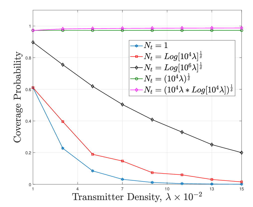
Fig. 6 shows the scaling of the coverage probability in ad hoc networks against the transmitter density for different scaling rates of the number of antennas; super-linear, linear, sub-linear, and constant (i.e, single antenna). We notice that the coverage decreases with the density for the single antenna case, as anticipated in (32), and also when the number of antennas is scaled sublinearly or linearly with the density, as predicted by Proposition 5. We observe that a super-linear scaling of the number of antennas with the BS density is required to prevent the SIR from dropping to zero, and thereby restore the SIR invariance property.

The impact of the BS height on the coverage probability is illustrated in Fig. 7. As predicted in Section IV.D, we note that a linear scaling of the number of antennas is required to maintain a non-zero SINR for low value of $h$ . When the BS height increases, the coverage probability decreases due to the increase of the path-loss and the linear scaling becomes insufficient.

VI Conclusion

By leveraging the properties of Fox’s H random variables, we developed a unifying framework to characterize the coverage probability of heterogeneous and muti-antenna networks under both the closest-BS and the strongest-BS cell association strategies. We studied the impact of BS densification on the coverage performance both under bounded and unbounded path loss models. By direct inspection of the obtained analytical framework, we have been able to derive exact closed-form formulations and scaling laws of the coverage probability for two typical network models, i.e., heterogeneous and multi-antenna cellular and ad hoc networks, while incorporating generalized fading distributions. The obtained results encompass insightful relationships between the BS density and the relative antenna array size, gain and height, showing how the coverage can be maintained whilst increasing the network density. The insights provided in this work are of cardinal importance for optimally deploying general ultra-dense networks.

VII Appendix A: Proof of Proposition 1

With the closest-BS association strategy, the coverage probability is given by

{\cal C}\triangleq\sum^{{\cal T}}_{k=1}{\cal\theta}_{k}{\cal P}\left(\text{SINR}_{k}>\beta_{k}\right),

(55)

where ${\cal\theta}_{k}$ denotes the association probability and is expressed as ${\cal\theta}_{k}=\frac{\lambda_{k}}{\sum_{j\in{\cal T}}\lambda_{j}\widetilde{P}_{j}^{\delta}}$ , and $\widetilde{P}_{j}=\frac{P_{j}}{P_{k}}$ . Using [10, Theorem 1] and [11, Eq. (39)] and applying the Fox’s $H$ -transform in [32, Eq. (2.3)], the coverage probability under unbounded path-loss model, denoted as ${\cal C}^{\cal U}$ , is given by

	$\displaystyle{\cal C}^{\cal U}(r_{k})$	$\displaystyle=$	$\displaystyle\int_{0}^{\infty}\frac{1}{\sqrt{\xi}}~{\cal L}^{-1}\left\{\frac{1}{\sqrt{s}}H_{p,q}^{u,v}\left\{f(t);{\mathcal{P}}\right\}(s\xi);s;{\cal\beta}_{k}\right\}$		(56)
			$\displaystyle e^{-\sigma^{2}_{k}\xi\frac{r_{k}^{\alpha}}{P_{k}}}\prod_{j\in{\cal T}}{\cal L}_{{\cal I}_{j}}\left(\xi\frac{r_{k}^{\alpha}}{P_{k}}\right)d\xi,$		(56)

where $f(t)=\sqrt{t}{\mathcal{J}}_{1}\left(2\sqrt{st\xi}\right)$ , $H_{p,q}^{u,v}\left\{f(t);{\mathcal{P}}\right\}(s)$ is the Mellin transform [32, Eq. (2.3)], ${\mathcal{J}}_{1}(x)=H_{0,2}^{1,0}\left(\frac{x^{2}}{4};(1,1,\frac{1}{2},-\frac{1}{2},1,1)\right)$ is the Bessel function of the first kind [38, Eq. (8.402)], and ${\cal L}^{-1}$ is the inverse Laplace transform. Moreover ${\cal L}_{{\cal I}_{j}}$ , in (62), is the Laplace transform of the aggregate interference from the $j$ -th tier evaluated as

{\cal L}_{{\cal I}_{j}}(s)=\exp(2\pi\lambda_{j}\Theta(s)),

(57)

where

$\displaystyle\!\!\Theta\mid_{H_{j}=y}(s)\!\!\!$	$\displaystyle\overset{(a)}{=}$	$\displaystyle\!\!\!\int_{\left(\frac{P_{j}}{P_{k}}\right)^{\frac{2}{\alpha}}r_{k}}^{\infty}\!\!\!\!\left(1-\exp\left(-syP_{j}r^{-\alpha}\right)\right)rdr$	(58)
		$\displaystyle\!\!\!\!\!\!\!\!\!\!\!\!\!\!\!\!\!\!\!\!\!\!\!\!\!\!\!\!\!\!\!\!\!\!\!\!\overset{(b)}{=}\frac{syP_{j}}{\alpha}\int_{\frac{P_{k}}{P_{j}}r_{k}^{-\alpha}}^{\infty}x^{-\frac{2}{\alpha}}e^{-syx}{\rm{}_{\!1}F_{\!1}}\left(1,2,syx\right)dx$
		$\displaystyle\!\!\!\!\!\!\!\!\!\!\!\!\!\!\!\!\!\!\!\!\!\!\!\!\!\!\!\!\!\!\!\!\!\!\!\!\overset{(c)}{=}\frac{syP_{j}~{\rm{}_{2}F_{2}}\left(1,-\frac{2}{\alpha}+1;2;-\frac{2}{\alpha}+2;-syP_{k}r_{k}^{-\alpha}\right)}{\left(\frac{P_{k}}{P_{j}}\right)^{\frac{2}{\alpha}-1}r^{(\alpha-2)}\alpha\left(\frac{2}{\alpha}-1\right)},$

where $(a)$ follows from the probability generating functional [9], [39], while relabeling $x$ as $r_{k}^{-\alpha}$ and $(1-e^{-x})/x=e^{-x}{\rm{}_{1}F_{1}}\left(1,2;x\right)$ is applied in $(b)$ , and $(c)$ follows from applying $\int x^{\beta-1}e^{-cx}{\rm{}_{1}F_{1}}(a,b,cx)=\frac{x^{\beta}}{\beta}{\rm{}_{2}F_{2}}\left(b-a,\beta,b,\beta+1,-cx\right)$ . Hence, we obtain

	$\displaystyle{\cal L}_{{\cal I}_{j}}(\xi)$	$\displaystyle=$	$\displaystyle\exp(-2\pi\lambda_{j}\mathcal{E}_{H_{j}}[\Theta(s)])$		(59)
			$\displaystyle\!\!\!\!\!\!\!\!\!\!\!\!\!\!\!\!\!\!\!\!\!\!\!\!\!\!\!\!\!\!\!\!\!\!\!\!=\exp\left(\!-\pi\delta\lambda_{j}\frac{\xi r_{k}^{2-\alpha}}{\left(1-\delta\right)}H_{p,q}^{u,v}\left\{g(t);{\mathcal{P}}\right\}(\xi)\!\right),$		(59)

where $g(t)=t~{\rm{}_{2}F_{2}}\left(1,1-\delta;2;2-\delta;-\xi tr_{k}^{-\alpha}\right)=tH_{2,3}^{1,2}\left(t;{\cal P}_{1}\right)$ , ${\cal P}_{1}=(1-\delta,\xi(r_{k}^{2})^{-\frac{\alpha}{2}},(0,\delta),(0,-1,\delta-1),{\bf 1}_{2},{\bf 1}_{3})$ , and ${\rm{}_{p}F_{q}}(\cdot)$ is the generalized hypergeometric function of [38, Eq. (9.14.1)]. In (59), in particular, we first take the expectation over the interferers’ locations and then average over the Fox’s H distributed channel gains, which is in the reverse order compared to the conventional derivations in [4]-[9]. The reason behind this order swapping is that the Fox’s H fading model is more complicated than the conventional exponential model, and therefore averaging over it in a latter step preserves the analytical tractability.

Finally, applying [32, Eq. (1.58)], the Mellin transform [32, Eq. (2.3)], and the inverse Laplace transform of the Fox’s $H$ -function [32, Eq. (2.21)] given by

{\cal L}^{-1}\{x^{-\rho}H_{p,q}^{u,v}(x;{\cal P});x;t\}=t^{-\rho-1}H_{p+1,q}^{u,v}\left(\frac{1}{t};{\cal P}_{l}\right),

(60)

where ${\cal P}_{l}=(\kappa,c,(a,\rho),b,(A,1),B)$ , the desired result is obtained after applying the Fox’s H reduction formulae in [32, Eq. (1.57)]. The coverage probability over Fox’s $H$ -fading⁴⁴ 4 We dropped the index $i$ from Fox’s $H$ -distribution $\{{\cal O}_{i},{\mathcal{P}}_{i}\}$ for notation simplicity. for a receiver connecting to a $k$ -th tier BS located at $x_{k}$ is given by

	$\displaystyle{\cal C}^{\cal U}(r_{k})\!\!$	$\displaystyle=$	$\displaystyle\!\!\int_{0}^{\infty}\frac{1}{\xi^{2}}H_{q,p+1}^{v,u}\left(\xi;{\cal P}^{k}_{\cal U}\right)e^{-\sigma^{2}_{k}\xi\frac{r_{k}^{\alpha}}{P_{k}}}$		(61)
			$\displaystyle\!\!\!\!\!\!\!\!\!\!\!\!\!\!\!\!\!\!\!\!\!\!\!\!\!\!\!\!\!\!\!\exp\Bigg(\!\!\!-\pi\delta\sum_{j\in{\cal T}}r_{k}^{2}\lambda_{j}\widetilde{P}_{j}^{\delta}\xi H_{q+2,p+3}^{v+1,u+2}\left(\xi;{\cal P}^{{\cal I}}_{\cal U}\right)\Bigg)d\xi,$		(61)

where $\widetilde{P}_{j}=\frac{P_{j}}{P_{k}}$ , $\delta=\frac{2}{\alpha}$ , and the parameter sequences ${\cal P}^{k}_{\cal U}=\!\!\left(\kappa{\cal\beta}_{k},\frac{1}{c{\cal\beta}_{k}},1\!-\!b,(1\!-\!a,1),\mathcal{B},(A,1)\right),$ and ${\cal P}^{{\cal I}}_{\cal U}=\bigg(\frac{\kappa}{c^{2}},\frac{1}{c},(1\!-\!b\!-\!2B,0,\delta),(0,1\!-\!a\!-\!2A,-1,\delta\!-\!1),$ $(\mathcal{B},1,1),(1,A,1,1)\bigg)$ . Recall that the pdf of the link’s distance $r_{k}$ is given by $f_{r_{k}}(x)=\frac{2\pi\lambda_{k}}{\theta_{k}}x\exp\left(-\sum_{j\in{\cal T}}\pi x^{2}\lambda_{j}\widetilde{P}_{j}^{\delta}\right)$ [3], [39]. Then recognizing that $\exp(-x)=H_{0,1}^{1,0}(x;{1,1,0,1,1,1})$ [32, Eq. (1.125)] in (61), we apply [32, Eq. (2.3)] to obtain the average coverage probability in (3) after some manipulations.

VIII Appendix B: Proof of Proposition 2

The proof of Proposition 2 relies on the same approach adopted in Appendix A, yielding

	$\displaystyle{\cal C}^{\cal B}(r_{k})\!\!\!\!$	$\displaystyle=$	$\displaystyle\!\!\!\!\int_{0}^{\infty}\frac{1}{\sqrt{\xi}}~{\cal L}^{-1}\left\{\frac{1}{\sqrt{s}}H_{p,q}^{u,v}\left\{f(t);{\mathcal{P}}\right\}(s\xi);s;{\cal\beta}_{k}\right\}$		(62)
			$\displaystyle e^{-\sigma^{2}_{k}\xi\frac{(1+r_{k})^{\alpha}}{P_{k}}}\prod_{j\in{\cal T}}{\cal L}_{{\cal I}_{j}}\left(\xi\frac{(1+r_{k})^{\alpha}}{P_{k}}\right)d\xi,$		(62)

where rearranging [11, Eq. (39)] after carrying out the change of variable relabeling $(1+x)^{-\alpha}$ as $x$ , we have

	$\displaystyle\!{\cal L}_{{\cal I}_{j}}(\xi)\!\!\!\!$	$\displaystyle=$	$\displaystyle\!\!\!\!\exp\!\!\Bigg(\!\!\!-\pi\delta\lambda_{j}\xi\Bigg(\!\!\frac{(1\!+\!r_{k})^{2-\alpha}}{\left(1-\delta\right)}H_{p,q}^{u,v}\!\!\left\{g_{1}(t);{\mathcal{P}_{1}}\right\}(\xi)-$		(63)
			$\displaystyle\frac{(1+r_{k})^{1-\alpha}}{\left(1-\frac{\delta}{2}\right)}H_{p,q}^{u,v}\left\{g_{2}(t);{\mathcal{P}}\right\}(\xi)\Bigg)\Bigg),$		(63)

where $g_{1}(t)=t~{\rm{}_{2}F_{2}}\left(1,1-\delta;2;2-\delta;-\xi t(1+r_{k})^{-\alpha}\right)$ and $g_{2}(t)=t~{\rm{}_{2}F_{2}}\left(1,1-\frac{\delta}{2};2;2-\frac{\delta}{2};-\xi t(1+r_{k})^{-\alpha}\right)$ . Finally applying the Mellin transform in [32, Eq. (2.3)] and plugging the obtained result into (62), Proposition 2 follows after some manipulations.

IX Appendix C: Proof of Proposition 3

Based on [11], the Laplace transform of the aggregate interference from tier $j$ under the max-SINR association strategy is evaluated as ${\cal L}_{{\cal I}_{j}}(\xi)=\exp\left(-\pi\lambda_{j}\xi^{\delta}\Gamma\left(1-\delta\right){\cal E}[H^{\delta}]\right)$ , where ${\cal E}[H^{\delta}]$ is the Mellin transform of the Fox’s- $H$ function obtained as ${\cal E}[H^{\delta}]=\Lambda$ [32, Eq. (2.8)]. Then following the analytical steps as in Appendix A, we obtain

$\displaystyle{\cal C}$	$\displaystyle=$	$\displaystyle\sum_{k\in{\cal T}}\lambda_{k}{\cal E}_{r_{k}}\Bigg\{\int_{0}^{\infty}\frac{1}{\xi^{2}}H_{q,p+1}^{v,u}\left(\xi;{\cal P}^{k}_{\cal U}\right)$
		$\displaystyle\exp\Bigg(-\sum_{j\in{\cal T}}r_{k}^{2}\pi\lambda_{j}\widetilde{P}^{\delta}_{j}\xi^{\delta}\Gamma(1-\delta)\Lambda_{j}\Bigg)d\xi\Bigg\}$
	$\displaystyle\overset{(a)}{=}$	$\displaystyle\sum_{k\in{\cal T}}\frac{\lambda_{k}}{\delta}{\cal E}_{r_{k}}\Bigg\{\int_{0}^{\infty}\frac{1}{\xi^{2}}H_{q,p+1}^{v,u}\left(\xi;{\cal P}^{k}_{\cal U}\right)$
		$\displaystyle\!\!\!\!\!\!\!\!\!\!\!\!\!\!\!\!\!\!\!H_{0,1}^{1,0}\!\!\left(\!\!\left(\!\sum_{j\in{\cal T}}r_{k}^{2}\pi\lambda_{j}\widetilde{P}^{\delta}_{j}\Gamma(1\!-\!\delta)\Lambda_{j}\!\!\right)^{\!\frac{1}{\delta}}\!\!\!\xi;\left(1,1,1,0,1,\frac{1}{\delta}\right)\!\!\right)\!\!d\xi\!\Bigg\},$

where $(a)$ follows from substituting $\exp(-x)=H_{0,1}^{1,0}(x;{1,1,-,0,-,1})$ [32, Eq. (1.125)] and applying the transformation $H_{p,q}^{u,v}\big[x\big|\begin{array}[]{ccc}(a_{i},kA_{j})_{p}\\ (b_{i},kB_{j})_{q}\end{array}\big.\big]=\frac{1}{k}H_{p,q}^{u,v}\big[x^{\frac{1}{k}}\big|\begin{array}[]{ccc}(a_{i},A_{j})_{p}\\ (b_{i},B_{j})_{q}\end{array}\big.\big]$ . Finally applying [32, Eq. (2.3)] yields the strongest-BS based coverage probability as shwon in Proposition 3.

References

[1] I. Trigui, S. Affes, M. Di. Renzo, D. N. K. Jayakody, ”SINR Coverage Analysis of Dense HetNetsOver Fox’s H-Fading Channels”, in Proc. IEEE Wireless. Commun. and Net. Conf. (WCNC), Seoul, South Korea, April 6-9, 2020.
[2] J. G. Andrews, S. Buzzi, W. Choi, S. Hanly, A. Lozano, A. C. Soong, and J. C. Zhang, ”What will 5G be?” IEEE J. Sel. Areas Commun., vol. 32, no. 6, pp. 1065–1082, June 2014.
[3] C. Li, J. Zhang, J. G. Andrews, and K. B. Letaief, ”Success probability and area spectral efficiency in multiuser MIMO HetNets,” IEEE Trans. Commun., vol. 64, no. 4, pp. 1544-1556, Apr. 2016.
[4] J. G. Andrews, F. Baccelli, and R. K. Ganti, ”A tractable approach to coverage and rate in cellular networks,” IEEE Trans. Commun., vol. 59, no. 11, pp. 3122-3134, Nov. 2011.
[5] M. Di. Renzo and P. Guan, “Stochastic geometry modeling of coverage and rate of cellular networks using the Gil-Pelaez inversion theorem.” IEEE Commun. Lett., vol. 19, no. 9, pp. 1575-1578, Sep. 2014.
[6] M. Di Renzo, A. Guidotti, and G. E. Corazza, “Average rate of downlink heterogeneous cellular networks over generalized fading channels: A stochastic geometry approach,” IEEE Trans. Commun., vol. 61, no. 7, pp. 3050-3071, Jul. 2013.
[7] Y. J. Chun, S. L. Cotton, H. S. Dhillon, A. Ghrayeb, and M. O. Hasna, ”A stochastic geometric analysis of device-to-device communications operating over generalized fading channels,” IEEE Trans. Wireless Commun., vol. 16, no. 7, pp. 4151-4165, Jul. 2017
[8] A. K. Gupta, H. S. Dhillon, S. Vishwanath, and J. G. Andrews, ”Downlink multi-antenna heterogeneous cellular network with load balancing,” IEEE Trans. Commun., vol. 62, no. 11, pp. 4052-4067, Nov. 2014.
[9] H. S. Dhillon, R. K. Ganti, F. Baccelli, and J. G. Andrews, ”Modeling and analysis of K-tier downlink heterogeneous cellular networks,” IEEE J. Select. Areas Commun., vol. 30, no. 3, pp. 550–560, Apr. 2012.
[10] I. Trigui, S. Affes, and B. Liang, ”Unified stochastic geometry modeling and analysis of cellular networks in LOS/NLOS and shadowed fading,” IEEE Trans. Commun., vol. 5, no. 99, pp. 1-16, July 2017.
[11] I. Trigui and S. Affes, ”Unified analysis and optimization of D2D communications in cellular Networks over fading channels”, IEEE Trans. Commun., early access, July 2018.
[12] M. Di Renzo, W. Lu, and P. Guan, ”The intensity matching approach: A tractable stochastic geometry approximation to system-level analysis of cellular networks,” IEEE Trans. Wireless Commun., vol. 11, no. 9, pp. 5963-5983, Sep. 2016.
[13] M. Di Renzo and P. Guan, ”A mathematical framework to the computation of the error probability of downlink MIMO cellular networks by using stochastic geometry,” IEEE Trans. Commun., vol. 62, no. 8, pp. 2860-2879, Aug. 2014
[14] M.G. Khoshkholgh and V. C. M. Leung, ”Coverage analysis of max-SIR cell association in hetNets under nakagami fading”, IEEE Trans. Vehic. Techn., vol. 67, no. 3, pp. 2420-2438. Mar. 2018.
[15] J. Liu, M. Sheng, L. Liu, and J. Li, ”Effect of densification on cellular network performance with bounded path-loss model,” IEEE Commun. Lett., vol. 21, no. 2, pp. 346-349, Feb. 2017.
[16] V. M. Nguyen and M. Kountouris, ”Performance limits of network densification,” IEEE J. Sel. Areas Commun., vol. 35, no. 6, pp. 1294-1308, Mar. 2017.
[17] M. Ding, P. Wang, D. López-Pérez, G. Mao, and Z. Lin, ”Performance impact of LoS and NLoS transmissions in dense cellular networks,” IEEE Trans. Wireless Commun., vol. 15, no. 3, pp. 2365-2380, Mar. 2016.
[18] I. Atzeni, J. Arnau, and M. Kountouris, ”Downlink cellular network analysis with LOS/NLOS propagation and elevated base stations,” IEEE Trans. Wireless Commun., vol. 17, no. 1, pp. 142-156, Jan. 2018.
[19] M. Filo, C. H. Foh, S. Vahid, and R. Tafazolli, ”Stochastic geometry analysis of ultra-dense networks: Impact of antenna height and performance limits.” [Online]. Available: https://arxiv.org/abs/1712.02235.
[20] N. Lee, F. Baccelli, and R. W. Heath, ”Spectral efficiency scaling laws in dense random wireless networks with multiple receive antennas,” IEEE Trans. Inform. Theory, vol. 62, no. 3, pp. 1344–1359, Mar. 2016.
[21] H. ElSawy, A. Sultan-Salem, M. S. Alouini, and M. Z. Win, ”Modeling and analysis of cellular networks using stochastic geometry: A tutorial,” IEEE Communications Surveys & Tutorials, vol. 19, no. 1, pp. 167-203, Firstquarter 2017.
[22] X. Zhang and J. G. Andrews, ”Downlink cellular network analysis with multi-slope path loss models,” IEEE Trans. Commun., vol. 63, no. 5, pp. 1881–1894, May 2015.
[23] R. K. Ganti and M. Haenggi, ”Asymptotics and approximation of the SIR distribution in general cellular networks,” IEEE Trans. Wireless Commun., vol. 15, no. 3, pp. 2130–2143, Mar. 2016.
[24] V. Chandrasekhar, M. Kountouris, and J. G. Andrews, ”Coverage in multi-antenna two-tier networks,” IEEE Trans. Wireless Commun., vol. 8, no. 10, pp. 5314–5327, Oct. 2009.
[25] A. M. Hunter, J. G. Andrews, and S. Weber, ”Transmission capacity of ad hoc networks with spatial diversity,” IEEE Trans. Wireless Commun., vol. 7, no. 12, pp. 5058–5071, Dec. 2008.
[26] G. George, R. K. Mungara, A. Lozano, and M. Haenggi, ”Ergodic spectral efficiency in MIMO cellular networks,” IEEE Trans. Wireless Commun., vol. 16, no. 5, pp. 2835–2849, May 2017.
[27] X. Yu, C. Li, J. Zhang, M. Haenggi, and K. B. Letaief, ”A unified framework for the tractable analysis of multi-antenna wireless networks,” IEEE Trans. Wireless Commun., vol. 17, no. 12, pp. 7965-7980, Dec 2018.
[28] M. Di Renzo and P. Guan, ”Stochastic geometry modeling and system-level analysis of uplink heterogeneous cellular networks with multi-antenna base stations,” IEEE Trans. on Commun., vol. 64, no. 6, pp. 2453-2476, Jun. 2016.
[29] M. Cheng, J.-B. Wang, Y. Wu, X.-G. Xia, K.-K. Wong, and M. Lin, ”Coverage analysis for millimeter wave cellular networks with imperfect beam alignment,” IEEE Trans. Veh. Technol., vol. 67, no. 9, pp. 8302-8314, Sep. 2018.
[30] X. Yu, J. Zhang, M. Haenggi, and K. B. Letaief, ”Coverage analysis for millimeter wave networks: The impact of directional antenna arrays,” IEEE J. Sel. Areas Commun., vol. 35, no. 7, pp. 1498-1512, Jul. 2017
[31] N. Deng, M. Haenggi, and Y. Sun, ”Millimeter-wave deviceto-device networks with heterogeneous antenna arrays,” IEEE Trans. Commun., vol. 66, no. 9, pp. 4271-4285, Sep. 2018.
[32] A. M. Mathai, R. K. Saxena, and H. J. Haubol, The H-function: Theory and Applications, Springer Science & Business Media, 2009.
[33] S. K. Yoo, S. Cotton, P. Sofotasios, M. Matthaiou, M. Valkama, and G. Karagiannidis, ”The Fisher-Snedecor F distribution: A simple and accurate composite fading model,” IEEE Commun. Letters, vol. 21, no. 7, pp. 1661-1664, July 2017.
[34] F. Yilmaz and M.-S. Alouini, ”A novel unified expression for the capacity and bit error probability of wireless communication systems over generalized fading channels,” IEEE Trans. Commun., vol. 60, no. 7, pp. 1862-1876, Jul. 2012
[35] M. Di Renzo and W. Lu, ”System-level analysis/optimization of cellular networks with simultaneous wireless information and power transfer: Stochastic geometry modeling,” IEEE Trans. Veh. Technol.,y, vol. 66, no. 3, pp. 2251–2275, Mar. 2017.
[36] M. Di Renzo, S. Wang, and X. Xi, ”Inhomogeneous double thinning— Modeling and analysis of cellular networks by using inhomogeneous Poisson point processes,” IEEE Trans. Wireless Commun., vol. 17, no. 8, pp. 5162-5182, Aug. 2018
[37] A. Kilbas and M. Saigo, H-Transforms: Theory and Applications, CRC Press, 2004.
[38] I. S. Gradshteyn and I. M. Ryzhik, Table of Integrals, Series and Products, 5th ed., Academic Publisher, 1994.
[39] M. Haenggi, Stochastic Geometry for Wireless Networks. Cambridge University Publishers, 2012

Instantaneous Fading Distribution	Coverage Probability ${\cal C}^{\cal U}$
Gamma Fading $f_{g}(z)=\frac{m}{\Gamma(m)}H_{0,1}^{1,0}\left[mz\left\|\begin{array}[]{ccc}-\\ (m-1,1)\end{array}\right.\right]$	$\begin{aligned} &{\cal C}^{\cal U}=\pi\delta\sum^{{\cal T}}_{k=1}\frac{\lambda_{k}m_{k}\beta_{K}}{\Gamma(m_{k})}\left(\frac{P_{k}}{\sigma_{k}^{2}}\right)^{\delta}\int_{0}^{\infty}\frac{H_{1,1}^{0,1}\left[\frac{\xi}{m_{k}\beta_{k}}\left\|\begin{array}[]{ccc}(2-m_{k},1)\\ (1,1)\end{array}\right.\right]}{\xi^{2+\delta}}\\ &{\mathcal{H}}_{1,1}^{1,1}\left(\!\!\frac{\left(\frac{P_{k}}{\sigma^{2}_{k}}\right)^{\delta}}{\xi^{\delta}}\!\!\sum_{j=1}^{\cal T}\!\!\!\pi\lambda_{j}\widetilde{P}^{\delta}_{j}\!\left(1\!+\!\frac{\delta\xi}{m_{j}\Gamma(m_{j})}H_{3,3}^{1,3}\!\!\left[\frac{\xi}{m_{j}}\left\|\begin{array}[]{ccc}(-m_{j},1),(0,1),(\delta,1)\\ (0,1),(-1,1),(\delta-1,1)\end{array}\right.\right]\right)\!,\!{\cal P}_{\delta}\!\!\right)\!d\xi\end{aligned}$

Generalized Gamma $\begin{aligned} &f_{g}(z)=\frac{\mu}{\Gamma(m)}H_{0,1}^{1,0}\left[\mu z\left\|\begin{array}[]{ccc}-\\ (m-\frac{1}{\eta},\frac{1}{\eta})\end{array}\right.\right]\end{aligned}$ where $\mu=\frac{\Gamma(m+\frac{1}{\eta})}{\Gamma(m)}$ .	$\begin{aligned} &{\cal C}^{\cal U}=\pi\delta\sum^{{\cal T}}_{k=1}\frac{\lambda_{k}\mu_{k}\beta_{K}}{\Gamma(m_{k})}\left(\frac{P_{k}}{\sigma_{k}^{2}}\right)^{\delta}\int_{0}^{\infty}\frac{H_{1,1}^{0,1}\left[\frac{\xi}{\mu_{k}\beta_{k}}\left\|\begin{array}[]{ccc}(1+\frac{1}{\eta_{k}}-m_{k},\frac{1}{\eta_{k}})\\ (1,1)\end{array}\right.\right]}{\xi^{2+\delta}}\\ &{\mathcal{H}}_{1,1}^{1,1}\left(\!\!\frac{\left(\frac{P_{k}}{\sigma^{2}_{k}}\right)^{\delta}}{\xi^{\delta}}\!\!\sum_{j=1}^{\cal T}\!\!\!\pi\lambda_{j}\widetilde{P}^{\delta}_{j}\!\left(1\!+\!\frac{\delta\xi}{\mu_{j}\Gamma(m_{j})}H_{3,3}^{1,3}\!\!\left[\frac{\xi}{\mu_{j}}\left\|\begin{array}[]{ccc}(1-\frac{1}{\eta_{j}}-m_{j},1),(0,1),(\delta,1)\\ (0,1),(-1,1),(\delta-1,1)\end{array}\right.\right]\right)\!,\!{\cal P}_{\delta}\!\!\right)\!d\xi\end{aligned}$

Power of Nakagami- $n$ (Rice) $\begin{aligned} &f_{g}(z)=\sum_{k=0}^{\infty}\frac{\Psi_{k}m_{k}}{\Gamma(m_{k})\Omega_{k}}H_{0,1}^{1,0}\left[\frac{m_{k}}{\Omega_{k}}z\left\|\begin{array}[]{ccc}-\\ (m_{k}-1,1)\end{array}\right.\right]\end{aligned}$ with $m_{k}=k+1$ and $\Omega_{k}=\frac{k+1}{1+K_{R}}$ , where $K_{R}$ is the Rician factor.	$\begin{aligned} &{\cal C}^{\cal U}=\pi\delta\sum^{{\cal T}}_{k=1}\underset{K_{k}\longrightarrow\infty}{\lim}\sum_{t=0}^{K_{k}}\frac{\Psi_{t}m_{t}}{\Gamma(m_{t})\Omega_{t}\lambda_{k}\beta_{k}}\left(\frac{P_{k}}{\sigma_{k}^{2}}\right)^{\delta}\int_{0}^{\infty}\frac{H_{1,1}^{0,1}\left[\frac{\xi\Omega_{t}}{m_{t}\beta_{k}}\left\|\begin{array}[]{ccc}(2-m_{t},1)\\ (1,1)\end{array}\right.\right]}{\xi^{2+\delta}}\\ &{\mathcal{H}}_{1,1}^{1,1}\!\!\left(\!\!\frac{\left(\frac{P_{k}}{\sigma^{2}_{k}}\right)^{\delta}}{\xi^{\delta}}\!\!\sum_{j=1}^{{\cal T}}\!\!\!\pi\lambda_{j}\widetilde{P}^{\delta}_{j}\!\left(1\!+\!\sum_{t=0}^{\infty}\frac{\Psi_{t}\Omega_{t}\delta\xi}{\Gamma(m_{t})m_{t}}H_{3,3}^{1,3}\!\!\left[\frac{\xi\Omega_{t}}{m_{t}}\left\|\begin{array}[]{ccc}(-m_{t},1),(0,1),(\delta,1)\\ (0,1),(-1,1),(\delta-1,1)\end{array}\right.\right]\!\right)\!,\!{\cal P}_{\delta}\!\!\right)\!d\xi\end{aligned}$ , where $\Psi_{k}=K_{R}^{k}e^{-K_{R}}/\Gamma(k+1)$ .

Lognormal Fading $\begin{aligned} &f_{g}(z)=\sum_{n=0}^{N}\frac{w_{n}}{\omega_{n}}H_{0,0}^{0,0}\left[\frac{z}{\omega_{n}}\left\|\begin{array}[]{ccc}-\\ -\end{array}\right.\right]\end{aligned}$ where $\omega_{n}=10^{\sqrt{2}\sigma u_{n}+\mu}$ , while $u_{n}$ and $w_{n}$ represrent the weight factors and the zeros of the $N$ -order Hermite polynomial [6, Table 25.10].	$\begin{aligned} &{\cal C}^{\cal U}=\pi\delta\sum^{{\cal T}}_{k=1}\sum_{t=0}^{N_{k}}\frac{w_{t}}{\omega_{t}\lambda_{k}\beta_{k}}\left(\frac{P_{k}}{\sigma_{k}^{2}}\right)^{\delta}\int_{0}^{\infty}\frac{H_{0,1}^{0,0}\left[\frac{\xi\omega_{t}}{\beta_{k}}\left\|\begin{array}[]{ccc}-\\ (1,1)\end{array}\right.\right]}{\xi^{2+\delta}}\\ &{\mathcal{H}}_{1,1}^{1,1}\!\!\left(\!\!\frac{\left(\frac{P_{k}}{\sigma^{2}_{k}}\right)^{\delta}}{\xi^{\delta}}\!\!\sum_{j=1}^{{\cal T}}\!\!\!\pi\lambda_{j}\widetilde{P}^{\delta}_{j}\!\left(1\!+\!\sum_{t=0}^{N_{j}}\frac{w_{t}\delta\xi}{\omega^{2}_{t}}H_{2,3}^{1,2}\!\!\left[\xi\omega_{t}\left\|\begin{array}[]{ccc}(0,1),(\delta,1)\\ (0,1),(-1,1),(\delta-1,1)\end{array}\right.\right]\!\right)\!,\!{\cal P}_{\delta}\!\!\right)\!d\xi\end{aligned}$

Fisher-Snedecor Fading $\begin{aligned} &f_{g}(z)=\frac{m}{m_{s}\Gamma(m_{s})\Gamma(m)}H_{1,1}^{1,1}\left[\frac{mz}{m_{s}}\left\|\begin{array}[]{ccc}(-m_{s},1)\\ (m-1,1)\end{array}\right.\right]\end{aligned}$	$\begin{aligned} &{\cal C}^{\cal U}=\pi\delta\sum^{{\cal T}}_{k=1}\frac{\lambda_{k}m_{k}\beta_{K}}{m_{s_{k}}\Gamma(m_{k})\Gamma(m_{s_{k}})}\left(\frac{P_{k}}{\sigma_{k}^{2}}\right)^{\delta}\int_{0}^{\infty}\frac{H_{1,2}^{1,1}\left[\frac{\xi m_{s_{k}}}{m_{k}\beta_{k}}\left\|\begin{array}[]{ccc}(2-m_{k},1)\\ (1+m_{s_{k}},1),(1,1)\end{array}\right.\right]}{\xi^{2+\delta}}\\ &{\mathcal{H}}_{1,1}^{1,1}\left(\!\!\frac{\left(\frac{P_{k}}{\sigma^{2}_{k}}\right)^{\delta}}{\xi^{\delta}}\!\!\sum_{j=1}^{{\cal T}}\!\!\!\pi\lambda_{j}\widetilde{P}^{\delta}_{j}\!\left(1\!+\!\frac{\delta\xi}{m_{j}\Gamma(m_{j})}H_{3,3}^{1,3}\!\!\left[\frac{\xi}{m_{j}}\left\|\begin{array}[]{ccc}(-m_{j},1),(0,1),(\delta,1)\\ (0,1),(-1,1),(\delta-1,1)\end{array}\right.\right]\right)\!,\!{\cal P}_{\delta}\!\!\right)\!d\xi\end{aligned}$

Coverage Analysis and Scaling Laws in Ultra-Dense Networks