Study of prompt emission of short gamma ray bursts using multi-color blackbody: a clue to the viewing angleJournal: ApJ
Abstract
The prompt emission of short gamma ray bursts (sGRBs) with known redshifts are analyzed using the model of multi-color blackbody which is interpreted as the emission from a non-dissipative photosphere taking into account a power law jet structure and the viewing geometry of the jet. We find nearly and of the sample are consistent with multi-color blackbody and a pure blackbody model, respectively. Using this interpretation, we infer that nearly of the sGRBs in our sample are observed within (or along the edge of) the jet core. The sGRB jets are deduced to possess a narrow core with a median . This suggests the rate of sGRBs that would be viewed within the jet core to be . The power law index of the decreasing Lorentz factor profile of the jet structure is deduced to be . The intrinsic luminosity is found to range between . The average values of Lorentz factor and nozzle radius of the sGRB jets are inferred to be and for the cases when the photosphere forms in the coasting (accelerating) phase respectively. The viability of the inferred values of the different parameters of the GRB outflow and viewing geometry within this physical interpretation, enhances the prospect of the photospheric emission model to explain the observed GRB spectrum.
Keywords:
Gamma ray bursts(629); Burst astrophysics(187); Gamma-ray transient sources(1853)I Introduction
A short Gamma ray burst (sGRB) is an extremely intense gamma ray flash that is observed for a duration of less than seconds (Kouveliotou et al. 1993). They are hypothesized to be produced by the merger of binary compact objects such as neutron star -neutron star and neutron star - black hole. The detection of gravitational waves along with GRB 170817A (Abbott et al. 2017a), has confirmed that at least a fraction of the observed sGRBs are produced by the merger of binary neutron stars. The extensive follow-up observations of the GRB 170817A have confirmed the following key aspects: (i) the presence of a relativistic jet (Mooley et al. 2018a; Mooley et al. 2018b; Duffell et al. 2018) ; (ii) the jet has some structure beyond the jet opening angle (Alexander et al. 2018) and (iii) it is viewed off-axis (Granot et al. 2018). This affirms that the observed prompt emission spectrum has a strong dependence on the viewing geometry and the structure of the jet. There are different possible jet structures such as Gaussian (Resmi et al. 2018; Troja et al. 2018; Cunningham et al. 2020), power law (Lundman et al. 2013; Gottlieb et al. 2021), hollow-cone (Takahashi & Ioka 2020a; Takahashi & Ioka 2020b) etc. Recent 3D simulation studies of the hydrodynamic evolution of the GRB jet as it penetrates through the stellar core, have found that it is more likely to form jet structures characterised by simple power law distributions (Gottlieb et al. 2020; Gottlieb et al. 2021).
The radiation process during the prompt emission of GRBs is still ambiguous. Because of the non-thermal nature of the spectrum, they are generally tried to be explained by the synchrotron emission process (Tavani 1996; Bošnjak et al. 2009; Yu et al. 2015; Zhang 2020). Recently, there have been several studies where a model of synchrotron emission is directly tested with the GRB data (Burgess et al. 2014; Burgess et al. 2020) as well as studies where doubly smoothly broken power laws are used to model the GRB spectra which later are interpreted as synchrotron emission (Oganesyan et al. 2017; Ravasio et al. 2018). Even though these works show that the GRB spectra can be fitted with synchrotron emission, it is worth noting that the microphysical parameters required to achieve these fits are either unrealistic or require some fine tuning. Thus, there are some major drawbacks in interpreting the GRB spectra as synchrotron radiation.
An alternative emission model that has been widely studied is the photosphere model. Photospheric emission is inherent in the classical fireball model where the thermalized emission from the photosphere forms a subdominant part of the entire prompt gamma ray emission (Mészáros 2006). The emission from the photosphere is expected to be completely thermalized, closely consistent with a blackbody spectrum, when no significant dissipation of the kinetic/ Poynting flux happens at moderate optical depths close to the photosphere. This is generally referred to as the non-dissipative photospheric emission (Ryde 2004; Ryde & Pe’er 2009; Guiriec et al. 2011; Axelsson et al. 2012; Iyyani et al. 2013; Acuner et al. 2019; Acuner et al. 2020). However, several studies have shown that if continuous or localized dissipation of the kinetic or Poynting flux energy happens at optical depths close to the photosphere can result in a non-thermalized emission which would look much broader than a Planck function (blackbody). These models are generally referred to as the subphotospheric dissipation models (Pe’er & Waxman 2004; Pe’er & Waxman 2005; Giannios 2006; Beloborodov 2013; Iyyani et al. 2015; Ahlgren et al. 2015; Ahlgren et al. 2019).
Lundman et al. 2013 studied the non-dissipative photospheric emission from relativistic jets that possess angle dependent Lorentz factor profile structure characterized by a power law distribution. They found that the observed emission from the photosphere can significantly alter from a blackbody spectrum depending on the viewing geometry and jet profile structure. The obtained spectrum is a superposition of several blackbodies with varying temperatures which brings about a significant broadening as well as softening of the low energy part of the spectrum below the peak. Their work, thus, predicted the low energy power law indices of the spectrum, expected from different power law distribution jet profiles when viewed outside the jet core.
The Band function is widely used to empirically model the prompt gamma ray emission of GRBs (Band et al. 1993). The low energy power law index of the Band function fits done to the short GRB spectra are largely found to be harder than the line of death () of synchrotron emission (Preece et al. 1998). This is demonstrated in the Figure 1a where we have plotted the distribution of of the Band function fits done to the time integrated emission (T90 region) of the short GRBs (blue) detected and reported by Fermi till 15th July 2018 in their spectral catalog. The plotted distribution includes only those cases where the is well constrained (i.e error measured on is less than ) and the peak energy, . This ensures that the hard values obtained in the spectral fits are not an artifact of having the close to the edge of the energy limits of the observation window. We find the mean of the of short (long) GRBs to be (). We also find that () of the short (long) GRBs possess an . Interestingly, we also note that () of these short (long) GRBs with hard values also possess steep high energy power law indices, . A similar assessment of distribution is also found in Dereli-Bégué et al. 2020 where they find that a significantly large fraction of the upper limit of in their sample violates the line of death of synchrotron emission. This kind of spectral features suggest a narrow spectrum and thereby strongly point towards the emission coming from the jet photosphere. In addition, the cluster analysis conducted on all Fermi detected GRBs by Acuner & Ryde 2018, found that the cluster that contains predominantly short bursts is found to be consistent with photospheric emission origin.
Testing the different physical models directly with spectral data would be the proper course of action, however, this process is computationally very intensive. In the traditional method of spectral analysis, the spectrum is analysed using different models and the best fit model is determined by the best fit statistics. However, we note that the spectral analyses of most of the GRB data show that many of the different empirical and physical models are statistically equally consistent with the data (Iyyani et al. 2016; Meng et al. 2018; Acuner et al. 2020) and as a result the best fit model remains ambiguous. In such scenarios of degeneracy between different models, the way forward will be to examine if the particular model of choice is consistent with the data and then assess the implications of the results within the physical interpretations of that model.
With these above motivations, in contrast to the traditional methodology, in this work, we first investigate if the time integrated as well as the peak count spectra of sGRBs with known redshifts, detected by Fermi gamma ray space telescope and Niel Gehrels Swift is consistent with the multi-color blackbody model or not. Later, this model is interpreted within the physical scenario presented in Lundman et al. 2013. The analysis results are presented in section II. The physical model and its correlation with the multi-color blackbody is described in section III. Within the physical interpretation, the assessment of the different parameters such as the viewing geometry, power law index of the Lorentz factor jet profile, the jet opening angle and the core angle of the jet are presented in section IV and section V. Finally, discussions and conclusions are presented in section VI and section VII respectively.
(b) The distributions of the high energy index, , of the Band function fits of the long and short GRB sample whose are shown. is marked by the vertical dotted line.
II Sample selection and spectral analyzes
All short GRBs with known redshifts detected by Fermi and Niel Gehrels Swift until December 2018 are included in our sample (see Table 1 for more details). This enables us to have strong constraints on the energetics of the bursts. However, this makes the sample a mixture of bursts with varying energy fluences ranging between orders of . The distribution of the redshift is shown in Figure 2a and we find the average redshift of the sGRBs to be (Berger 2014).
Niel Gehrels Swift BAT (Burst Alert Telescope) data is available for all sGRBs in the sample except for GRB 170817A. There are 12 sGRBs which are observed by both Fermi and Niel Gehrels Swift BAT and in these cases, joint spectral analyzes are done using the prompt emission data from both the missions and composite light curves are made (see Figures 14,15,16,17 in appendix). For BAT data analyzes, the light curves and spectra are generated using the standard procedures11 1 https://swift.gsfc.nasa.gov/analysis/threads/bat threads.html and data within the energy range keV are used. For Fermi data analyzes, the three bright sodium iodide (NaI) detectors with source angles and the brightest bismuth germanate (BGO) detector are chosen and data within energy ranges, NaI: keV; BGO: keV - MeV are used22 2 For GRB 090510, Fermi Large Area Telescope low energy (LLE) data was available and the data in the energy range were used in the spectral analyzes.. The Fermi spectral files are generated using Burst Analysis GUI v 02-01-00p1 (gtburst3)33 3 https://fermi.gsfc.nasa.gov/ssc/data/analysis/scitools/gtburst.html.
The time interval for integrated spectral analysis is chosen subjectively by looking at each burst lightcurve such that it includes the entire prompt emission of the burst. The start and stop times of the intervals as well as the results of the spectral analyzes are mentioned in Table 2. The interval used for time integrated analysis of each burst is marked in shaded red color in the burst lightcurves shown in Figures 14, 15, 16, 17 in appendix. The time integrated analyzes enables us to model the average shape of the overall burst emission and thereby estimate the total isotropic energy of the burst, (Table 2). We assume a flat universe with cosmology parameters: = 67.4, = 0.315 and for estimating the luminosity distances (Aghanim et al. 2018). The distribution of the estimated is shown in Figure 2b and we find the average isotropic total energy of sGRBs to be .
The burst emission can undergo significant spectral evolution within the total duration of the burst and therefore, the underlying actual spectrum can be identified by doing time resolved spectral analysis. However, the brevity of sGRBs makes the time resolved spectral analysis highly challenging due to photon scarcity in each time resolved interval. Therefore, in this work, we conduct the spectral analysis of the peak count interval of each burst where the photon counts are the highest. Since the sample consists of sGRBs of varying intensity, we employ signal-to-noise ratio (SNR)44 4 The Bayesian block binning method, on the other hand, primarily follows the changes in counts of the light curve to decide the time intervals. In case of a sGRB with low intensity, this method may not give us a peak count spectral time interval with enough signal-to-noise ratio to constrain the spectral model parameters. binning method on the BAT light curves which are available for all sGRBs except GRB 170817A where the method is employed on the brightest NaI detector. Later from the time resolved bins, the interval with highest counts is identified for spectral analysis. The start and stop times of the intervals as well as the results of the spectral analyzes are mentioned in the Table 3. The interval used for peak count spectral analysis of each burst is marked in shaded black color in the burst light curves shown in Figures 14, 15, 16, 17 in Appendix. We point out that a strict limit of SNR could not be exercised on the entire sample because of the varying intensity of the bursts. Thus, we choose the best possible SNR values subjectively for each burst such that the overall variability of the light curve is retained and enough signal is obtained in the peak interval to constrain the spectral parameters of most of the models that are fitted. The SNR values ranging between are used for different bursts to obtain their respective peak count spectrum (see the table 8 in appendix).
The spectral analyzes are conducted on both the time integrated and time resolved peak count spectra of each burst using the Multi-Mission Maximum Likelihood (3ML) software (Vianello et al. 2015). We use the maximum likelihood estimation technique to estimate the best fit spectral parameters and follow Akaike Information Criteria (AIC) for model selection (Akaike 1974).
II.1 Results of spectral analyzes
We analyze the time integrated and the peak count spectra of each burst in our sample using the empirical models such as power law (PL), power law with exponential cutoff (CPL), Band function (Band) and physical models like blackbody (BB) and multicolor blackbody (mBB, the model named as diskpbb in Xspec. See the section III for more details). The functions of the different models are given in the appendix A. We note that the aim of this spectral analyzes is to inspect if physical models like multi-color blackbody or simple blackbody can fit the data consistently or not, and does not aim to rule out other possible interpretations to the same data.
The spectral fits of the different models are compared by estimating the , where is the AIC obtained for each spectral model (see Table 6 and Table 7 in appendix for time integrated and peak spectral analyzes respectively) and is the minimum of the AIC values obtained for all the spectral models that are in comparison. The is estimated for each burst and is plotted in Figure 3.
Generally, the plausible models are those whose (region shown in dark grey area), those models with in the light grey area have inconclusive evidence and those models with in the white area are considered implausible (Burnham et al. 2011). We note that most of the tried models are largely consistent with the data, which leads to the scenario of degeneracy between models (see Figure 18 in Appendix). Since the best fit model is ambiguous in this work, we consider the limit of to determine if the model of our choice i.e mBB or BB is consistent with the data or not. If we find the or , then we choose or as the best fit model of the respective spectral analysis. If , then the model with the least is chosen as the best fit model for that analyzes. The results for the time integrated and peak count spectra are shown in Table 2 and Table 3 respectively. With this methodology, we find that the peak count spectra of GRB 101219A and GRB 060801 are best modeled using PL model, whereas the remaining sGRBs in the sample are found to be consistent with either mBB or BB model. We find that of the sample is consistent with multi-color blackbody spectrum, whereas of the sample is consistent with a simple blackbody spectrum. Thus, only GRBs in the sample whose peak count spectra are consistent with either mBB or BB are studied further within the structured jet model. Throughout the paper, until otherwise mentioned, the spectrum used for study is only the peak count spectrum.
II.2 Results of Multi-color Blackbody (mBB) fits
The appropriate method would have been to directly fit the output of the Monte Carlo simulations of the Lundman et al. 2013 model with the data, however, this process is computationally very intensive and also, time consuming when it has to be employed on a large sample of bursts. In addition, it has also been shown in several studies (Iyyani et al. 2016; Meng et al. 2018; Acuner et al. 2020) that different physical models can be equally fitted to the data, thereby being unable to resolve the ambiguity between different spectral models that are analysed. In this scenario, we find it judicious to use the readily available multi-color blackbody, diskpbb, model adopted from Xspec whose spectral shape is produced by the superposition of many blackbodies analogous to that expected in Lundman et al. 2013. This diskpbb model was originally devised to model the spectrum coming from an accretion disc. Therefore, we note that the interpretations that we do to this model in the current work are totally different and have no connection other than the similar spectral shapes.
The multi-color blackbody has three fit parameters: is the peak temperature (keV), is the power law index of the radial dependence of the temperature55 5 For a different formulation, refer Hou et al. 2018, wherein instead of probability distribution of temperatures, they consider a multi-color blackbody whose distribution of luminosity is a function of temperature with a power-law form. In contrast to diskpbb, in their model, they have the minimum temperature, also as a free parameter, thereby allowing the inclusion of the Rayleigh-Jean component of the spectrum below , in the modelling of the observed spectral data.
| (1) |
and is the normalization (the detailed model expression is given in the Appendix A). The parameter space of is configured to (the default range is for the accretion disk, Makishima et al. 1986) in order to incorporate the wide range of spectral shapes that are possible in case of the GRB spectra. The minimum and maximum values obtained in this sample study are and respectively. When tends to infinity, theoretically the tends to a spectral shape. The mBB spectral shapes obtained for different and are plotted in the Figure 4.
We simulate a large number of mBB spectral model assuming normal distributions for the fit parameters with the best fit values as the mean and the errors as its standard deviation. For each instance of the simulated mBB spectral model, a power law model is fitted to the low energy part of the spectrum below and thus, the power law spectral index (mBB ) corresponding to a given mBB spectral shape is measured. This is repeated for all the simulated mBB spectra and thereby obtaining a distribution of mBB . We then fit a Gaussian function to this distribution to obtain the mean as the mBB value and the standard deviation as its error.
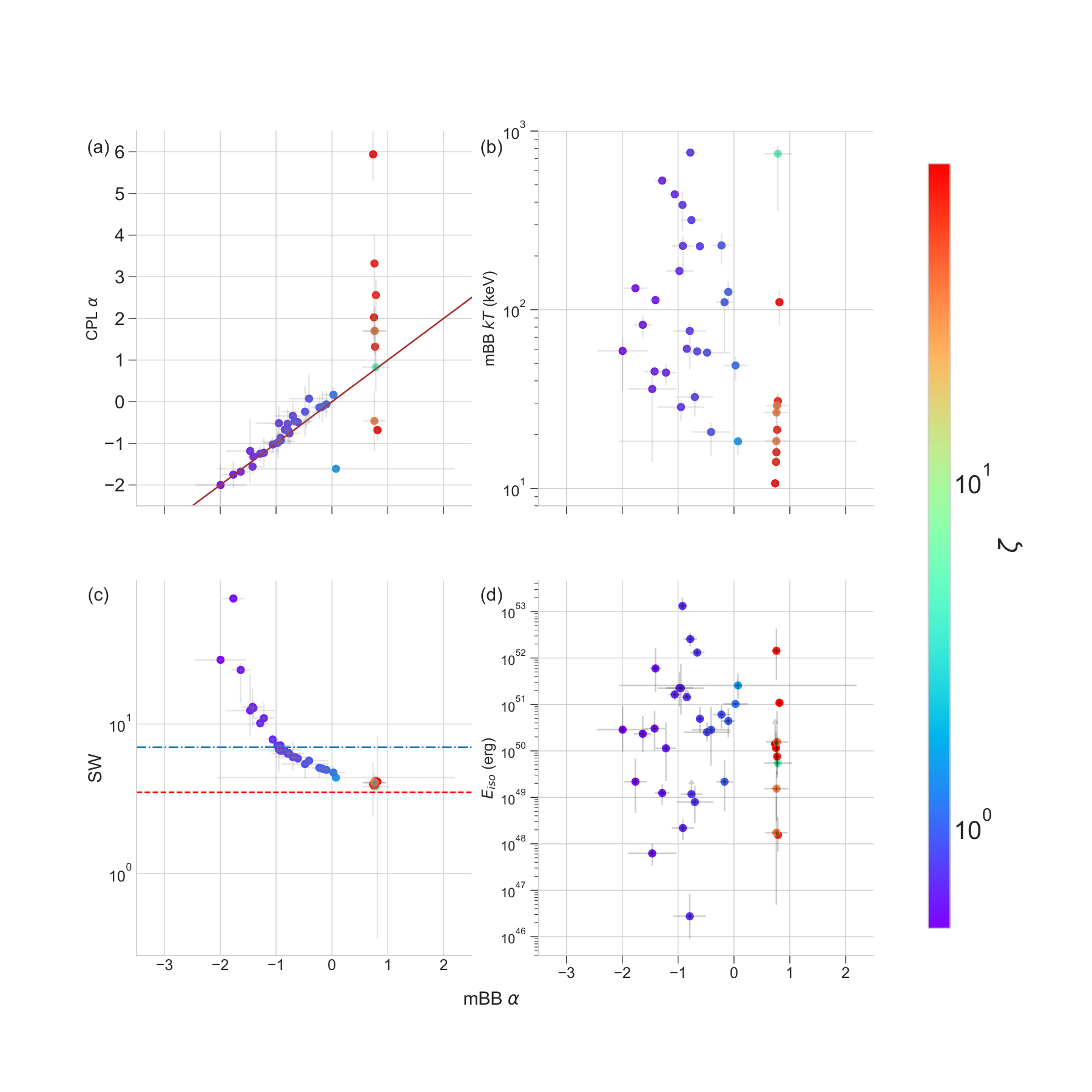
The mBB model is flexible enough to capture the spectral features, similar to the empirical model CPL. This comparison is shown in the Figure 5a where the low energy power law indices, CPL , of cutoff power law function are plotted against the low energy power law indices, mBB , obtained for the multi-color blackbody fits. We find that the spectra with soft low energy spectral slopes () are consistently reproduced by both the models within errors. However, we find that the spectra which tend to have hard spectral slopes () are not well captured by CPL mostly in cases where the peak of the spectrum is also close to the edge of the energy window, which results in unphysical hard CPL values66 6 The narrowest spectrum that can be obtained is that of a blackbody (Planck function) whose low energy spectral slope is . On the other hand, these hard spectra when modeled using mBB produce good fits and has values which are more realistic. This shows that CPL is not always a good enough empirical approximation for blackbody model particularly when the model finds it difficult to constrain the cutoff peak energy at low energies close to the edge of the energy window.
We note that there is no correlation found between the peak temperature, of mBB fits with the spectral slope, mBB (Figure 5b) indicating that there is no energy window bias. We also studied the spectral width77 7 Spectral width is defined as the ratio of the limiting energies bounding the full width half maximum of the spectral peak (Axelsson & Borgonovo 2015; Iyyani et al. 2015) of the mBB model fits. We find that as gets harder, the width of the spectrum becomes narrower. A significant fraction of the GRBs have peak count spectrum that is as narrow as the non-dissipative photospheric emission from a spherically symmetric wind () and even narrower as blackbody () (Iyyani et al. 2015). The broadest spectrum is found to be of (the errors on the spectral width are not well constrained in this case) with the softest in the sample. We note that we do not find any spectral width as large as a few hundreds as expected in the fast cooling synchrotron emission (power law electron distribution; ) and slow cooling synchrotron emission (Maxwellian electron distribution; ) (Axelsson & Borgonovo 2015; Iyyani et al. 2015). We also do not find any correlation between the isotropic burst energy, and mBB (Figure 5d). It is interesting that a given has a large range of of at least order of magnitude. This suggests that the intrinsic total burst energy of the sGRB events vary case to case.
III Structured Jet
The observations of GRB 170817A have affirmed that a successful relativistic jet surrounded by a mildly relativistic structure was produced in the sGRB event (Mooley et al. 2018a; Kathirgamaraju et al. 2018). Previously, several hydrodynamic simulations have shown that as the jet emerges out, by undergoing significant interactions with its surrounding ejecta (or stellar core in case of long GRBs), the jet develops some angular profile structure with varying Lorentz factor, mass density and total energy (Zhang et al. 2003; Morsony et al. 2007; Mizuta et al. 2011). Inspired by these simulations, Lundman et al. 2013 did a Monte Carlo simulation of the non-dissipative photospheric emission from a structured jet with an angular Lorentz factor profile such that within the jet core, the Lorentz factor remains constant and beyond the core, the Lorentz factor decreases as a power law until the jet opening angle88 8 When the core region extends till , the jet structure becomes equivalent to a top-hat jet. (, see Figure 6). The Lorentz factor profile structure is analytically defined as the following
| (2) |
where is the Lorentz factor of the outflow within the jet core, , is the power law index of the decreasing Lorentz factor profile beyond the and is the lowest Lorentz factor (slightly differing from unity) considered in the above definition of the jet profile. In this structured jet model, the outflow luminosity per solid angle of the central engine is considered to be angle independent99 9 The observed jet luminosity, however, would decrease with increasing viewing angle (Lundman et al. 2014). within and thereby, the outflow temperature at the nozzle radius, , also remains angle independent. Beyond there is no injection of burst energy (Figure 6) and therefore, any observer at a viewing angle, , would not see any prompt emission from the GRB. Such a luminosity profile is inspired by the hydrodynamical simulations presented in Zhang et al. 2003.

They computed the observed spectrum from the photosphere when it forms in the coasting phase (that is the photosphere lies above the saturation radius), taking into account the jet angular profile and the geometry of how the jet is viewed by the observer. They found that when a jet is viewed off-axis along the edge or beyond the jet core, such that the emission from the wings of the jet significantly contribute to the resultant spectrum, the observed spectrum from the photosphere is much broader than a pure blackbody () with the low energy part of the spectrum below the peak energy as soft as . The broadening of the observed spectrum from a pure blackbody is due to the fact that the resultant spectrum is a superposition of multiple blackbodies of decreasing temperatures coming from the emitting regions of lower Lorentz factors. However, when viewed within the jet core, the spectrum is found to be relatively narrower with a low energy power law index , similar to the spectrum expected from a spherical wind (Beloborodov 2011).
III.1 Correlation between mBB and the structured jet
Lundman et al. 2013 model found that for values of , the low energy power law index of the observed spectrum, is related to the jet’s Lorentz factor profile index, by the relation
| (3) |
in case of a narrow jet (where ) such that the observed emission is dominated by the emission coming from the region outside the jet core and thereby depends on the profile of the structure of the jet. In case of a wide jet ( ), when viewed within the jet core (), the observed emission has minimum superposition of blackbodies of varying temperatures, and the spectrum would be close to a thermal shape (). Even in case of wide jets, if viewed outside or close to the jet core (), the spectrum would be dominated by the emission coming from the region of decreasing Lorentz factor and this would produce significant softening in the low energy part of the spectrum.
From the mBB spectral fits, we find that is linearly correlated to . Using a linear fit, we find the correlation to be
| (4) |
and is shown in the Figure 7a. We note that deviates from this linear relationship. This deviation arises because when equals large values, it means that the temperature varies steeply, thereby, producing less softening of the spectrum below the peak. As a result, the spectrum tends towards a blackbody (see Figure 4). Due to the limiting value of , we do not find a corresponding increase in for large values of . By equating equations 3 and 4, we find the relation between the fit parameter, and the Lorentz factor profile index, to be
| (5) |
We estimate the values by using this relationship and the values obtained from the multi-color blackbody fits. The estimates are shown in the Figure 7b as a function of . We note that , gives negative values of which suggest an increasing Lorentz factor profile structure beyond the jet core. However, even in such a jet profile structure, if viewed outside the jet core, the spectrum would be expected to have softer values. On the other hand, the hard values of suggest that there is less emission from outside the jet core contributing to the observed spectrum. We, thus, note that the negative values obtained in these cases are not physically feasible and is obtained as the result of the break down of the approximate relation between and found in Lundman et al. 2013. Also, for values of gives rise to large values of which suggests a top hat jet and in which case, the jet would be visible only when it is viewed within the jet cone. Thus, these hard values and the corresponding values clearly indicate that these spectra are obtained when viewed within the jet core. For gives values of which suggest that the decrease of the Lorentz factor beyond the jet core is very weak, in other words, no significant decrease in exists beyond the jet core. One possibility is that such spectrum is obtained by viewing a narrow jet () on-axis such that within the viewing cone a significant part of the emission is from the region outside the jet core. Lundman et al. 2013 have shown that such scenarios can produce spectrum with very soft value. However, considering (see section VI.3), we find that in such cases, which is unlikely. Another possibility is that the peak count spectra that are studied in these cases could be the integration of evolving spectra in the time bin, leading to soft values. It is, thus, likely that in these cases the underlying instantaneous spectrum may possess an .
The jet profile structure can be estimated only if the observed spectrum is shaped dominantly by the emission coming from the regions outside the jet core. The physically reasonable range of values that can be derived, thus, lie between which corresponds to values ranging between to as suggested in Lundman et al. 2013. These regions are marked in shaded green color and the curve (blue solid line) corresponding to the equation 3 is shown in the Figure 7b. The values of versus are plotted in the Figure 7c.
IV Determination of the viewing angle,
Following the above discussion, the viewing geometry, whether the GRB is viewed within or outside the jet core, is assessed using the following criteria:
(i) GRBs with observed determined from the mBB spectral fits1010
10
We note that can also be obtained when wider jets are viewed near or outside the edge of the jet core (Lundman et al. 2013; Meng et al. 2019, also see section IV.2)., and the non-observance of jet break in the afterglow emission are classified to possess a narrow jet with the line of
sight of the observer lying outside the jet core angle,
.
(ii) Those GRBs with spectral index, or has a jet break in the afterglow
emission are classified as GRBs that are viewed within the core of the jet.
We find that GRBs ( of the sample) are viewed from outside the and the remaining GRBs in the sample are viewed within the jet core.
IV.1 GRBs viewed outside the jet core and distribution of
With this understanding, we then estimate the viewing angle, of the GRBs that are viewed from outside the jet core, using the X-ray afterglow emission observed by X-ray Telescope (Figure 19 in appendix). When the afterglow emission produced by a structured jet is viewed off-axis, the peak of the afterglow light curve is observed when . Let and be the timescales of afterglow emission as observed by the observer who is placed on-axis and off-axis from the direction of the jet respectively. The ratio of these timescales are given as (Granot et al. 2002). When the peak of the emission is observed (i.e ), we find that and when , we find where where is the radius from where the afterglow emission is observed and it is measured from the center of the GRB explosion.
In most of these cases except GRB 170817A and GRB 150101B, the afterglow emission consists of decreasing flux which suggests that the peak of the emission has already gone past the start time () of the XRT afterglow observations and what we are observing is the decay phase. This means and by equating
| (6) |
we estimate the at the which we denote as as the Lorentz factor at the time of peak emission would have been greater than this value. Since the of XRT observations in these GRBs are only a few hundred seconds, we can consider that the has not significantly evolved to larger values from the radius of deceleration. We, thus, assume and estimate the . Since during the decay phase, , thus, with the above estimate of the Lorentz factor, we find the probable range of viewing angle to be and the values obtained are reported in the Table 4.
In GRB 170817A and GRB 150101B, the peak of the afterglow emission is observed at and 1111 11 __ (we consider this peak even though it is not statistically very significant in the data). Such long time after the onset of afterglow emission suggests that and should have significantly decreased and increased with time respectively. In case of GRB 170817A (GRB 150101B), by assuming that the initial Lorentz factor and following the standard afterglow emission properties in Huang et al. 2000, we expect to have increased from a deceleration radius of by an order of and Lorentz factor would have decreased to by the time, when the peak of the afterglow emission has been observed by the observer. The Lorentz factor at has to , this brings in a constraint that () which gives a () which in turn constraints the viewing angle to be () for GRB 170817A (GRB150101B), where the upper limit of (Nagakura et al. 2014). We note that the robust way to determine the viewing angle would be by modeling the afterglow data directly using the physical models. The above mentioned method gives only a rough estimate of the probable viewing angles. We also note that there were not enough XRT data points to allow us to make the estimations of , and for GRB 100206A, GRB 090417A and GRB 070923A.
For these GRBs that are viewed outside the jet core (also the cases where the jet is viewed along the edge of the jet core, see section IV.2), the Lorentz factor jet profile () is found from the relation given in equation 5 and the possible range is determined by taking into account the errors of and . The values are reported in the Table 4 and Table 5. In order to get a generic perspective of what the jet profile index would be, we made a cumulative distribution of the possible values of by assuming a uniform distribution between the minimum and maximum values of the estimated for each GRB. The obtained cumulative distribution is shown in Figure 8. We find the most probable peak at and a secondary peak at . We further note that from Figure 5a, the measured from CPL (the empirical model) and the mBB fits are similar and consistent with each other when the low energy spectrum is mostly soft. Since, the is estimated for , we note that the estimates done here are, therefore, largely spectral model-independent.
IV.2 GRBs viewed within the jet core
Depending on the burst dynamics, the optical depth of the outflow may fall to unity either below or above the saturation radius (), thereby leading to the formation of the photosphere in either the accelerating or coasting phase respectively. When viewed within the jet core, the spectrum expected from the photosphere formed in the coasting phase would possess an . On the other hand, the spectrum expected from the photosphere formed in the accelerating phase would possess a more harder spectrum which would be closely similar to a blackbody (Beloborodov 2011; Ryde et al. 2017).
Out of the GRBs that are viewed within the jet core, we find 10 GRBs in which mBB fits produce extremely narrow spectra with (Figure 5(a)) and they are found to be equally consistent with BB. We find that in some of these cases BB gives a much lower AIC than mBB, however, we find that the values of both models are within . This is mainly because BB has lower number of free parameters in comparison to mBB. A pure blackbody is not expected from a GRB outflow (Ryde et al. 2017) and therefore, we find the mBB fits to be more physically reasonable. Such extremely narrow and hard spectrum is expected from a photosphere formed in the accelerating phase.
Based on the observance of jet breaks, the following GRB 160821B, GRB 140903A, GRB 090510, GRB 061201 and GRB 051221A are included as cases where the jet is viewed within the jet core even though they possess . These soft can be understood as the artifact of two possibilities: (i) the jet may be viewed close to the core edge such that the emission from higher latitudes with lower Lorentz factors become significant, thereby softening the low energy part of the spectrum; (ii) due to poor signal-to-noise ratio, it is likely that there is significant integration of time dependent variation of the spectrum within the analyzed peak time interval which thereby leads to softer .

V Determination of the jet opening angle, and jet core,
V.1 GRBs viewed outside the jet core
In case of GRBs that are viewed outside the jet core, the possible range of is considered as those values such that . In case of GRB 170817A, we have considered the possible range of values to be between based on the values that were earlier reported in the literature by modeling the afterglow emission (D’Avanzo et al. 2018). The obtained values are listed in Table 4. Figure 10(a) shows the cumulative probability density distribution of the possible range of estimates of made from the GRBs that are viewed outside the jet core. We find that the median of the distribution is and the most probable value of is .
In GRBs that are viewed outside the jet core, we cannot make a clear estimate about the jet opening angle, , but the possible range would be between , which is the hard upper limit of the jet opening angle (Nagakura et al. 2014).
V.2 GRBs viewed within the jet core
In our sample, there are GRBs (GRB 051221A, GRB 061201, GRB 090426, GRB 090510, GRB 130603B, GRB 140903A, GRB 160821B) with jet breaks ( respectively) that have been previously reported and studied as well. Among them apart from GRB 090426 and GRB 130603B, all others have .
The afterglow light curves produced by the structured jet with profiles similar to the one discussed in this work, when viewed outside the jet core are expected to exhibit an increasing flux which later on at a point in time turns over and start decreasing. This jet break is associated to the point when the Lorentz factor along the line of sight of the observer becomes equal to . In contrast to this behaviour, in the above 7 GRBs in our sample, a decreasing light curve and a sharp jet break is observed later in time. This suggests that these GRBs are viewed within the jet core, . In such cases, the observed jet break refers to the scenario when (Peng et al. 2005) 1212 12 The jet break corresponding to is likely to be smeared out and less distinguishable in the afterglow light curve (Peng et al. 2005). Thus, wherever the jet break is observed in the afterglow emission in this sample, the opening angle of the jet is estimated using the standard formula given in Sari et al. 1999; Wang et al. 2015 which is based on the temporal evolution of the during the afterglow,
| (7) |
where is the radiation efficiency, is the number density of the ambient medium () and is the time of jet break observed in the afterglow emission measured in days. In this work, the jet opening angle of these GRBs are estimated using the following methodology: for the unknown parameters, we adopted a uniform distribution for between values of , a lognormal distribution for with the mean value (mean of the median values estimated in Fong et al. 2015) with a standard deviation of and a uniform distribution for between the minimum and maximum values found in Table 2. Using these inputs, we found a normal distribution of possible values for these GRBs (for an example see the Figure 20a in appendix). The mean and standard deviation obtained from these distributions are used to report the possible range of values of these GRBs in Table 5. We find these to be nearly consistent with the previous estimates reported in the literature.
In short GRBs, only a handful of cases show a distinct jet break in their afterglow emission and most of the GRBs show a single power-law decline. In our study, we have GRBs that are viewed within the jet core, out of which GRBs do not possess a jet break in their afterglow emission. We estimate the jet opening angle in these cases using the condition of jet collimation as the jet drives itself out of the surrounding, mildly relativistic expanding ejecta that is produced as a result of the NS-NS merger. Nagakura et al. 2014 conducted a hydrodynamic study of this propagation of the jet and found that the jet undergoes collimation at the least in the vicinity of the central engine where the ejecta is the densest. The density of the ejecta () in NS-NS merger events are found to decrease steeply with radius such that where (Hotokezaka et al. 2013). Bromberg et al. 2011 had done an analytical analysis of the interaction between the relativistic jet and the surrounding stellar mantle in case of long GRBs and found out that the condition for collimation1313 13 As shown in Bromberg et al. 2011, for values of the jet is likely to be uncollimated. However, at radius, , the jet is likely to be collimated at the least once and later as the density decreases, the jet may not undergo any further collimation and in this work our aim is to find the maximum limiting value of . is where is the ratio of jet energy density (, where is the jet luminosity and is the jet cross-section, and rest mass energy density of the ejecta at the jet head (), and is the initial jet opening angle as the jet starts. As the jet interacts with the surrounding ejecta, it heats up the ambient matter which in turn applies pressure on the jet which leads to collimation. The degree of collimation decreases as the density of the ambient ejecta decreases. Close to the nozzle radius of the jet, the density of the ejecta is high enough to collimate the jet at least once and thus, the resultant jet opening angle, would be lower than but is generally found to be larger than (Mizuta & Ioka 2013).
The expression for is expanded by including the analytical model of the ejecta profile obtained from the numerical simulations of Hotokezaka et al. 2013 and is given in equation 6 in Nagakura et al. 2014. We thus find the jet opening angle, , by the following expression
| (8) |
where is the isotropic luminosity, is the ejecta mass, is the time taken to launch the jet, where is the radius from where the jet starts and . We estimate the value at which can be associated to the nozzle radius of the jet (, see section VI.3) and therefore in the above equation and , which thus, makes the above equation independent of .
The time, can be splitted into three main parts (Zhang 2019; Beniamini et al. 2020): time taken for the black hole to form (), time taken for the accretion disk to form and start accreting () and finally, the time taken to launch the jet (, where is the velocity of the jet at which is relatively very low and we assume a Lorentz factor of ). We consider a uniform distribution for mass of the ejecta between limits of . With these inputs into the equation 8, we find the possible distribution of such that and . The distribution is found to be uniform and thus, the upper limit of is taken as . The lower limit of is equal to the estimate made using the last time of observation in case of a single power law decline of afterglow emission and if no significant afterglow emission data is available, then the estimate is made from the distribution of . The distribution of is found to be roughly Gaussian and thereby the mean and standard deviation are estimated (for an example see Figure 20b in appendix). Thus, in such cases equals the minimum value of including its error. The hard upper limit of is considered as as in the simulations of Nagakura et al. 2014 it was found that the jet launched with was not able to penetrate through the ejecta. This is because a large cross-section leads to lower and thereby becomes unsuccessful to push aside the ejecta and eventually expands quasi-spherically.
The possible range of of GRBs, thus, observed within the core of the jet are presented in the Table 5. Figure 10(b) shows the cumulative probability density distribution of the possible range of estimates of . We find the median of the distribution to be and the most probable is .

VI Discussion
VI.1 Jet opening angle and viewing geometry
The large isotropic energies estimated for the gamma ray burst requires that the outflow is emitted within a certain solid angle, thereby bringing the energetics in accord with known brightest explosions in the universe such as a supernova. Since, the outflow possesses very high Lorentz factors of the order of a hundred, the observer views only the emission within and when , the emission can be considered as isotropic. However, when the jet crashes into the afterglow emission and starts to decelerate, increases which eventually results in a scenario where , thereby revealing the edge of the jet emission. This results in a steeper decay of observed flux of the afterglow emission. With this understanding, we have been modeling the breaks observed in the decaying afterglow emission, where the emission transitions into a post break phase where the power law index of the decay becomes steeper than and sometimes, even as steep as the accelerated electron energy power law index in case of sideways expansion of the jet (Sari et al. 1999). In cases, where no jet break was found, the last data point was considered to estimate the lower limit on the jet opening angle. This has been the standard procedure for estimating the opening angle of the GRB jet.
The main difference of this work from the previous studies of Fong et al. 2013a; Fong et al. 2015 is that in their works they considered that all the observed sGRB jets are top-hat and thereby are viewed within the jet core (). The possibility of a structured jet and a viewing geometry of the jet outside the jet core were not considered. In this work, while analysing the prompt emission of sGRBs we have taken into account both these above factors. The viewing geometry of the different sGRBs in our sample are inferred using the methodologies described in sections IV and V and the result is demonstrated in the Figure 9.
The cumulative density distribution of the uniform distribution assumed between the minimum and maximum of the probable values of and estimated for the different sGRBs in the sample that are viewed outside and inside the jet core are plotted in the Figure 10(a) and 10(b) respectively. We find the median jet core angle, is and the median of jet opening angle, is . Thus, this study shows that the core of the jet of sGRBs can be very narrow (see also Beniamini et al. 2019). This finding is consistent with the observational evidence found from the modeling of the afterglow emission of GRB 170817A (Mooley et al. 2018a) where the GRB jet core is found to be as narrow as . On the other hand, the median of jet opening angle, is largely consistent with the results of Fong et al. 2015.
Taking into consideration the estimates of the possible viewing angles of the sGRBs presented in the section IV, we plot the cumulative distribution of and find that the probability to observe a sGRB within the jet core is and the probability to observe the GRB along the edge of the jet core () is around . Thus, we find that when the possibility of the jet having a structure is taken into consideration, the probability to observe the GRB jet along the edge is quite significant and we find this consistent with what has been anticipated by Lundman et al. 2013 (also see Beniamini & Nakar 2019).
Based on the detection of GW 170817A by LIGO and VIRGO (Abbott et al. 2017a), the rate of binary neutron star mergers are estimated to be . The brightest GRBs can be observed when the core of the jet is pointed towards the observer. The rate of sGRB events that would be viewed within the jet core is estimated by
| (9) |
Using the information of the from the current study, is estimated to be and events per for the most probable and median values of the distribution respectively. Considering the full LIGO sensitivity, the gravitational waves from sGRBs can be detected up to a luminosity distance of which would correspond to a co-moving volume of . This predicts the rate of very bright sGRB events that would be detected with the jet core pointed towards the observer to be and events per year for the most probable and median values of the distribution respectively.
VI.2 Correlation between burst energetics and peak temperature
We first study the correlation between the obtained peak temperatures, of the mBB fits with the observed energy flux, . In case of sGRBs whose mBB fits are close to that of the blackbody, we find a power law correlation such that . Excluding these cases, the remaining sGRBs with mBB fits exhibit a power law correlation of (see Figure 11a). We note that both the correlations are consistent with each other. In a relativistically expanding outflow, the observed thermal flux () and temperature () is expected to follow the correlation such as
| (10) |
where which represents the transverse size of the emitting region (photosphere). It can vary from burst to burst and also, during a burst emission. Thus, the observed thermal flux is expected to vary from the expected emergent flux () from the photosphere (Ryde 2004; Ryde & Pe’er 2009).
In this study, we find that of the sample is viewed within the jet core and is consistent with mBB fit. This provides a strong assessment of the total intrinsic energy of the jet and we find that the isotropic energy of the bursts varies between . Figure 11b shows that there is no strong correlation that can be ascertained between the peak temperature () and . Using the average value of the possible estimated for each GRB (section V), we also estimate the jet opening angle corrected burst energy, of the GRBs that are viewed within the jet core, which we find to vary between . Again, we do not find any strong correlation between the and (Figure 11b). These observations are found to be consistent with the sample study of sGRBs conducted by Dereli-Bégué et al. 2020.
The sGRBs that are considered to be viewed outside the jet core, also do not show any particular correlation between and . At the same time, we find that estimates of these sGRBs vary between erg. The brightest cases are those viewed close to the edge of the jet wherein a significant decrease in the Lorentz factor of the jet has not occurred. This is evident in the Figure 12 where we find that by considering the upper limit of the possible range of , most of the sGRBs viewed outside the jet core are likely to be viewed within . However, we note that the actual is unknown as in most cases we do not have an absolute estimate of these parameters instead we only know the possible range of values.
VI.3 Jet Outflow parameters
Among the sGRBs that are viewed within the jet core, sGRBs possess and are nearly consistent with BB. These cases are interpreted as the emission coming from the photosphere formed in the accelerating phase of the jet. The outflow parameters of these sGRBs are estimated using the methodology described in Bégué & Iyyani 2014. The different outflow parameters such as the photospheric radius, , Lorentz factor of the outflow at the photosphere, , nozzle radius of the jet, , saturation radius, and the maximum Lorentz factor attainable at , are estimated and plotted in Figure13. We find that the average values of , , , and .
The other sGRBs with softer are considered as the emission from the photosphere formed in the coasting phase. In these cases of mBB fits, we extract the blackbody component corresponding to the peak temperature, and estimate the respective blackbody flux which are then used in the calculations to estimate the outflow parameters of the jet using the methodology given in Pe’er et al. 2007; Iyyani et al. 2013. The obtained outflow parameters are shown in the Figure 13. We find that the average values of , , and 1414 14 In the coasting phase, the Lorentz factor of the outflow at the photosphere, is equal to . . We note that our estimates of Lorentz factors are relatively lesser than those reported in Dereli-Bégué et al. 2020 where they find the average value to be . The major difference being that redshift is not known for most of the bursts in their sample and they had thus assumed a common redshift value of for the estimations of .
We note that in both the scenarios, the photosphere forms roughly at the similar radius of the order of and the coasting Lorentz factor, and the are also found to be consistent with each other. This is also reflected in the consistent mass ejection rate observed in both the scenarios (Figure 13). The major difference is observed in the outflow parameter of the nozzle radius, of the jet which in the case of accelerating phase, is found to be nearly two orders of magnitude larger than that in the case of the photosphere forming in the coasting phase. This large value of basically pushes the saturation radius to higher values, which eventually lets the formation of the photosphere in the accelerating phase. Such large values of have been previously estimated in case of long GRBs, where the has been found to increase from radius close to the vicinity of the central engine to a large radius comparable to the size of the stellar core (Iyyani et al. 2013; Iyyani et al. 2016). The nozzle radius of the jet represents the radius from where the jet starts accelerating. As the jet drives through the surrounding ejecta, it is possible that the kinetic energy of the jet attained till then gets dissipated due to strong oblique shocks created by the interaction between the jet and the surrounding ejecta. Since the photon producing processes such as Bremsstrauhlung, double Compton etc are very efficient at these low radius and due to high optical depths, the dissipated energy is thermalized such that apparently a new fireball is formed at a larger radius which then starts accelerating more freely (Thompson et al. 2007; Iyyani et al. 2013; Iyyani et al. 2016). With this understanding, we find that the sGRBs with photosphere forming in the accelerating phase tend to have strong oblique or collimation shocks as the jet interacts with the surrounding ejecta than in those sGRBs with their photospheres in the coasting phase.
VI.4 Alternate interpretations
VI.4.1 Synchrotron emission
The non-thermal nature of the GRB spectra has been inspirational in modeling the emission by synchrotron. The dissipation of the kinetic energy/ Poynting flux of the jet by internal shocks/ magnetic reconnections in the optically thin region in the outflow, heat electrons and in some cases, accelerate them to a power law distribution which eventually cools by radiating via synchrotron. If the magnetic fields are strong, then the electron cool on a timescale less than the dynamical time required by the electrons to cross the region of shock. This is referred as fast cooling synchrotron emission which can explain . If the magnetic field strength is weak, then the shocked electrons cool on a timescale greater than the dynamical time. This is referred as the slow cooling synchrotron emission which can explain spectra with . Synchrotron emission produced within its conventional microphysical parameters’ space, cannot produce which is referred as the ’line of death’ of synchrotron emission. However, in a recent study by Burgess et al. 2019 (also see Oganesyan et al. 2019) have shown that synchrotron emission can produce consistent fits to even very hard spectra with . Their study shows that synchrotron emission can explain GRB spectra with a wide range of values. However, it has been noted that in such cases, the synchrotron emission models require extremely large emission radius which suggests very high ratio of total burst energy to the ambient matter density (Ghisellini et al. 2020). There have also been attempts to model the prompt emission spectra using doubly broken power law model which is interpreted as synchrotron emission (Oganesyan et al. 2017; Ravasio et al. 2018; Ravasio et al. 2019). In this interpretation, the double breaks observed in the GRB spectra are considered as the cooling frequency () and the minimum frequency () of synchrotron spectrum. To get these breaks consistently in the X-ray regime and a small ratio of would require a fine tuning in the microphysical parameters such that the synchrotron radiation remains in the marginally fast cooling regime (Beniamini et al. 2018). Proton-synchrotron emission, on the other hand, seems to alleviate many of these issues (Ghisellini et al. 2020).
The hard spectral slopes, , had been attempted to be explained by synchrotron self-absorption. However, in order to obtain the synchrotron self-absorption frequency, , in the X-ray regime, extreme conditions such as very high Lorentz factor () and magnetic fields () are required to obtain the system to be optically thick to synchrotron emission even when it is optically thin to Thompson scattering and pair creation (Granot et al. 2000; Lloyd & Petrosian 2000). In addition, if we consider the electrons to be cooling, then it is required that either (fast cooling) or (slow cooling). In this scenario, these extreme values of the Lorentz factor and magnetic fields push the synchrotron peak () to higher energies of the order of a few GeV which would severely violate the energy budget of the GRB. We also note that synchrotron emission spectrum from a relativistic Maxwellian electron distribution is found to have a spectral width of (Axelsson & Borgonovo 2015). Most of the sGRB spectra in our sample are much narrower than this limit (also see Burgess 2019).
VI.4.2 Subphotospheric dissipation
Photospheric emission is inherently anticipated in the classical fireball model (Mészáros 2006; Bégué et al. 2013; Bégué & Vereshchagin 2014). Even though photospheric emission can relieve many limitations of the synchrotron emission such as the narrow range of peak energy, high radiation efficiency etc, it was challenging to explain the GRB spectra which looked non-thermal in nature which were not very narrow as the blackbody emission expected from the photosphere. This led to the approach of considering the possibility of dissipation of kinetic/ Poynting flux happening below the photosphere. If the dissipation of the kinetic/ Poynting flux of the jet happens either continuously or at localized regions below the photosphere such that thermalization of the emission is not fully achieved, in such cases the emission from the photosphere is found to possess extremely non-thermal shapes (Pe’er & Waxman 2004; Ryde et al. 2010; Beloborodov 2013; Iyyani et al. 2015; Ahlgren et al. 2015; Bhattacharya et al. 2018; Ahlgren et al. 2019; Bhattacharya & Kumar 2020). Such emission spectra are found to consistently fit the observed data with soft values. Therefore, subphotospheric dissipation is one of the key alternate explanations for the sGRB spectra in our sample with soft .
VI.4.3 Cocoon emission
Several numerical simulation studies (Lazzati et al. 2017) have shown that the sGRB jets emerging from NS-NS mergers are likely to be surrounded by a mildly relativistic cocoon. In the scenario where the GRB jet is viewed off-axis, the observed prompt emission can be composed of the emission coming from the cocoon. This transient X-ray emission from the cocoon is expected to be either thermal or a Comptonised spectrum. Below we discuss if the multicolor blackbody spectra presented in this work can be produced by the cocoon or not.
Lazzati et al. 2017 found that the emission from the cocoon is expected to have a peak photon energy which is in contrast to the high peak temperatures that are observed in our sample (). Also, the isotropic energy from the cocoon is expected to be which is again in contrast to the majority of the isotropic burst energies observed for the sGRBs in our sample.
VII Conclusions and summary
The detection of the gravitational waves along with the short GRB 170817A marked the onset of multi-messenger astronomy-astrophysics. In addition, extensive observations were carried out for the afterglow across various wavelengths such as radio, optical and X-rays. GRB 170817A was an atypical event in terms of both the prompt as well as afterglow emission because of its low luminosity and delayed onset and steadily rising afterglow emission respectively. The event affirmed certain aspects of gamma ray burst such as the presence of a jetted emission with a significant structure beyond its core and in addition that the event is viewed at an angle significantly away from the axis of the jet. This suggests that the observed prompt gamma ray emission of a GRB event depends on the above two aspects. In addition, a large fraction of the time integrated sGRB gamma ray spectra are found to possess , the line of death of synchrotron emission, along with steep indices for the high energy part of the spectra. These spectral features suggest that the observed emission is more likely from a photosphere.
All the above factors, thus motivated us to analyze the sGRB prompt gamma ray bursts’ spectra using the multi-color blackbody model which is interpreted as the non-dissipative photospheric emission from a jetted outflow with a power law decreasing Lorentz factor profile outside the jet core, accounting for different viewing angles. We find that sGRBs in our sample (sGRBs with known redshifts) are consistent with this model interpretation. From the spectral fits, we find that sGRBs in the sample are observed outside the jet core whereas out of the remaining sGRBs that were viewed within the jet core, cases had emission consistent from that of the photosphere produced in the coasting phase and other cases where the emission was consistent with photosphere formed in the accelerating phase. From the spectral fits of the cases where the burst was viewed off jet core and close to the edge of the jet core, we infer the power law index of the Lorentz factor jet profile to be most probably between . The study of the outflow dynamics of the sGRBs viewed on-axis shows that the average Lorentz factor and the nozzle radius of the jet is deduced to be in case of photosphere forming in the coasting (accelerating) phase.
The opening angle of the jet in cases where the jet break was observed is estimated using the standard formula, however, wherever the break was not observed we estimated the possible range of the jet opening angle using the condition of jet confinement as the jet drives out through the surrounding ejecta. The median value of distribution is deduced to be . In case of GRBs observed outside the jet core, the jet core angle is estimated using the condition . With these estimates, the most probable (median) value of the distribution of the is inferred to be (). Thus, our study shows that sGRBs tend to possess very narrow jet cores consistent with the observations of GRB 170817A. The predicted rate of sGRB events that can be detected by LIGO with jet core pointed towards the observer is inferred to be events per year for .
In this study, we, thus, demonstrate that analyzing the sGRB spectra using a simple non-dissipative photospheric emission model accounting for the jet structure and viewing geometry allows us to assess the viewing angle as well as the power law behaviour of the angle dependent Lorentz factor profile of the jet.
We also note that the inferred values of the different parameters of the GRB outflow are physically reasonable and viable. This justifies our consideration of non-dissipative photospheric emission model including the geometrical broadening for analyzing the prompt emission of sGRBs, as well as enhances the probability of this physical model in giving rise to the observed short GRB spectra. This conclusion entitles for further investigation of sGRB spectra using photospheric emission models including different Lorentz factor jet profile structures via numerical simulations. In addition, the viability of this physical interpretation of the spectral data and the limitations faced by the synchrotron model on the other hand, allows us to speculate that the outflow is likely to be baryon dominated which implies that the remnant of the merger of the binary neutron stars maybe a black hole rather than a magnetar. In the era of multi-messenger astronomy, this notion can be confirmed with future observations and analysis of both electromagnetic and gravitational waves detected from sGRBs.
We would like to thank Prof. Felix Ryde, Dr. Christoffer Lundman and Prof. Dipankar Bhattacharya for insightful discussions and comments on the manuscript. We would also like to thank the anonymous referee for the very insightful and valuable suggestions which have considerably improved the manuscript. This work has made use of data supplied by the UK Swift Science Data center at the University of Leicester and Fermi data obtained through High Energy Astrophysics Science Archive Research Center Online Service, provided by the NASA/ Goddard Space Flight Center.
| GRB name | Tstart | Tstop | / | /kT | Flux () | () | Chosen |
|---|---|---|---|---|---|---|---|
| (s) | (s) | (keV) | (erg/cm2/s) | (erg) | Best fit model | ||
| 170817A | -0.37 | 2 | mBB | ||||
| 170428A | -0.1 | 0.5 | mBB | ||||
| 161104A | -0.3 | 0.1 | - | PL | |||
| 160821B | -0.15 | 0.6 | mBB | ||||
| 160624A | -0.4 | 0.4 | mBB | ||||
| 150423A | -0.3 | 0.3 | mBB | ||||
| 150120A | -0.9 | 2.1 | mBB | ||||
| 150101B | -0.2 | 0.02 | mBB | ||||
| 141212A | -0.12 | 0.6 | mBB | ||||
| 140903A | -0.7 | 0.8 | mBB | ||||
| 140622A | -0.2 | 0.2 | BB | ||||
| 131004A | -0.4 | 1.8 | Band | ||||
| 130603B | -0.12 | 0.25 | mBB | ||||
| 120804A | -0.3 | 2.6 | mBB | ||||
| 111117A | -0.3 | 1.1 | mBB | ||||
| 101219A | -0.4 | 1 | - | PL | |||
| 100724A | -0.4 | 1.56 | mBB | ||||
| 100628A | -0.3 | 0.04 | BB | ||||
| 100625A | -0.2 | 0.7 | mBB | ||||
| 100206A | -0.1 | 0.2 | mBB | ||||
| 100117A | -0.1 | 0.3 | mBB | ||||
| 090927 | -0.3 | 2.8 | mBB | ||||
| 090515 | -0.4 | 0.1 | BB | ||||
| 090510 | -0.565 | 0.395 | mBB+PL | ||||
| 090426 | -0.4 | 1.5 | mBB | ||||
| 090417A | -0.2 | 0.07 | BB | ||||
| 080905A | -0.11 | 1.21 | mBB | ||||
| 071227 | -0.7 | 2.2 | mBB | ||||
| 070923 | -0.3 | 0.1 | mBB | ||||
| 070729 | -0.2 | 1 | - | mBB | |||
| 070724A | -0.2 | 0.6 | mBB | ||||
| 070429B | -0.4 | 0.7 | mBB | ||||
| 061217 | -0.3 | 0.6 | mBB | ||||
| 061201 | -0.2 | 1.1 | - | PL | |||
| 060801 | -0.2 | 0.5 | mBB | ||||
| 060502B | -0.1 | 0.2 | mBB | ||||
| 051221A | -0.2 | 2.1 | - | PL | |||
| 050813 | -0.3 | 0.5 | BB | ||||
| 050509B | -0.2 | 0.1 | mBB |
Note: For mBB, BB and Band fits, the energy flux is reported for the energy range keV - MeV, however for PL fits, the energy flux is reported for the energy range for Niel Gehrels Swift BAT detected GRBs.
| GRB name | Tstart | Tstop | Flux () | Chosen | |||
| (s) | (s) | (keV) | (erg/cm2/s) | Best fit model | |||
| 170817A | -0.32 | 0.256 | mBB | ||||
| 170428A | 0.23 | 0.26 | mBB | ||||
| 161104A∗ | -0.13 | 0.03 | () | () | () | () | BB (mBB) |
| 160821B | -0.08 | 0.04 | mBB | ||||
| 160624A | -0.1489 | 0.1294 | mBB | ||||
| 150423A | -0.0713 | 0.1644 | mBB | ||||
| 150120A | 0.22 | 0.392 | mBB | ||||
| 150101B | -0.0914 | 0.0186 | mBB | ||||
| 141212A | -0.0336 | 0.3264 | mBB | ||||
| 140903A | -0.326 | 0.0544 | mBB | ||||
| 140622A∗ | -0.0520 | 0.1480 | () | () | () | () | BB (mBB) |
| 131004A | 0.041 | 0.0974 | mBB | ||||
| 130603B | -0.05 | 0.023 | mBB | ||||
| 120804A | 0.3 | 0.4 | mBB | ||||
| 111117A | 0.35 | 0.47 | mBB | ||||
| 101219A | -0.18 | 0.06 | - | - | PL | ||
| 100724A | 0.0031 | 0.486 | mBB | ||||
| 100628A∗ | -0.14 | 0.04 | () | () | () | BB (mBB) | |
| 100625A∗ | 0.17 | 0.2 | () | () | () | () | BB (mBB) |
| 100206A | -0.03 | 0.05 | mBB | ||||
| 100117A | -0.02 | 0.11 | mBB | ||||
| 090927 | 0.03 | 0.46 | mBB | ||||
| 090515∗ | -0.19 | 0.04 | () | () | () | () | BB (mBB) |
| 090510 | -0.27 | 0.028 | mBB | ||||
| 090426∗ | 0.43 | 0.53 | () | () | () | () | BB (mBB) |
| 090417A | -0.1 | 0.04 | mBB | ||||
| 080905A∗ | 0.9565 | 0.9781 | () | () | () | () | BB (mBB) |
| 071227 | 0.226 | 0.465 | mBB | ||||
| 070923 | -0.14 | 0.04 | mBB | ||||
| 070729 | 0.08 | 0.2 | mBB | ||||
| 070724A | 0.0064 | 0.2736 | mBB | ||||
| 070429B | 0.02 | 0.21 | mBB | ||||
| 061217∗ | -0.081 | 0.155 | () | () | () | () | BB (mBB) |
| 061201 | 0.38 | 0.55 | mBB | ||||
| 060801 | -0.1 | 0.1 | - | - | PL | ||
| 060502B | -0.06 | 0.04 | mBB | ||||
| 051221A | -0.07 | 0.1 | mBB | ||||
| 050813∗ | -0.07 | 0.27 | () | () | () | () | BB (mBB) |
| 050509B∗ | -0.08 | 0.02 | () | () | () | () | BB (mBB) |
∗ The GRBs whose spectra are consistent with BB.
| GRB name | |||||
|---|---|---|---|---|---|
| 170817A | |||||
| 150423A | |||||
| 150120A | |||||
| 150101B | |||||
| 141212A | |||||
| 120804A | |||||
| 111117A | |||||
| 100724A | |||||
| 100206A | |||||
| 100117A | |||||
| 090927 | |||||
| 090417A | |||||
| 071227 | |||||
| 070923 | |||||
| 070729 | |||||
| 070724A |
| GRB name | ||||
|---|---|---|---|---|
| 170428A | - | |||
| 161104A | - | |||
| 160821B | a | |||
| 160624A | - | |||
| 140903A | b | |||
| 140622A | - | |||
| 131004A | - | |||
| 130603B | c | - | ||
| 100628A | - | |||
| 100625A | - | |||
| 090510 | ||||
| 090515 | - | |||
| 090426 | e | - | ||
| 080905A | - | |||
| 070429B | - | |||
| 061217 | - | |||
| 061201 | f | |||
| 060502B | - | |||
| 051221A | g | |||
| 050813 | - | |||
| 050509B | - |
a Jin et al. 2018 has reported a .
b Troja et al. 2016 has reported a .
c Fan et al. 2013 and Fong et al. 2014 have reported and .
d Corsi et al. 2010 and Fraija et al. 2016 have estimated a .
e Guelbenzu et al. 2011 has reported a (n is assumed to be ).
f Stratta et al. 2007b has reported a .
g Soderberg et al. 2006 has reported a .
References
- Abbott et al. (2017a) Abbott, B. P., Abbott, R., Abbott, T. D., et al. 2017a, ApJ, 848, L13, doi: 10.3847/2041-8213/aa920c
- Abbott et al. (2017b) —. 2017b, ApJ, 848, L12, doi: 10.3847/2041-8213/aa91c9
- Acuner & Ryde (2018) Acuner, Z., & Ryde, F. 2018, MNRAS, 475, 1708, doi: 10.1093/mnras/stx3106
- Acuner et al. (2020) Acuner, Z., Ryde, F., Pe’er, A., Mortlock, D., & Ahlgren, B. 2020, ApJ, 893, 128, doi: 10.3847/1538-4357/ab80c7
- Acuner et al. (2019) Acuner, Z., Ryde, F., & Yu, H.-F. 2019, MNRAS, 1306, doi: 10.1093/mnras/stz1356
- Aghanim et al. (2018) Aghanim, N., Akrami, Y., Ashdown, M., et al. 2018, arXiv preprint arXiv:1807.06209
- Ahlgren et al. (2015) Ahlgren, B., Larsson, J., Nymark, T., Ryde, F., & Pe’er, A. 2015, MNRAS, 454, L31, doi: 10.1093/mnrasl/slv114
- Ahlgren et al. (2019) Ahlgren, B., Larsson, J., Valan, V., et al. 2019, ApJ, 880, 76, doi: 10.3847/1538-4357/ab271b
- Akaike (1974) Akaike, H. 1974, in Selected Papers of Hirotugu Akaike (Springer), 215–222
- Alexander et al. (2018) Alexander, K. D., Margutti, R., Blanchard, P. K., et al. 2018, ApJ, 863, L18, doi: 10.3847/2041-8213/aad637
- Axelsson & Borgonovo (2015) Axelsson, M., & Borgonovo, L. 2015, MNRAS, 447, 3150, doi: 10.1093/mnras/stu2675
- Axelsson et al. (2012) Axelsson, M., Baldini, L., Barbiellini, G., et al. 2012, The Astrophysical Journal Letters, 757, L31
- Band et al. (1993) Band, D., Matteson, J., Ford, L., et al. 1993, The Astrophysical Journal, 413, 281
- Barthelmy et al. (2005) Barthelmy, S., Barbier, L., Cummings, J., et al. 2005, GRB Coordinates Network, 3385, 1
- Barthelmy et al. (2006) Barthelmy, S. D., Burrows, D. N., Chester, M. M., et al. 2006, GRB Coordinates Network, 5926, 1
- Baumgartner et al. (2009) Baumgartner, W. H., Barthelmy, S. D., Cummings, J. R., et al. 2009, GRB Coordinates Network, 9138, 1
- Beardmore et al. (2017) Beardmore, A. P., Kuin, N. P. M., Page, K. L., et al. 2017, GRB Coordinates Network, 21042, 1
- Beardmore et al. (2009) Beardmore, A. P., Kennea, J. A., Markwardt, C. B., et al. 2009, GRB Coordinates Network, 9356, 1
- Bégué & Iyyani (2014) Bégué, D., & Iyyani, S. 2014, ApJ, 792, 42, doi: 10.1088/0004-637X/792/1/42
- Bégué et al. (2013) Bégué, D., Siutsou, I. A., & Vereshchagin, G. V. 2013, ApJ, 767, 139, doi: 10.1088/0004-637X/767/2/139
- Bégué & Vereshchagin (2014) Bégué, D., & Vereshchagin, G. V. 2014, MNRAS, 439, 924, doi: 10.1093/mnras/stu011
- Beloborodov (2011) Beloborodov, A. M. 2011, ApJ, 737, 68, doi: 10.1088/0004-637X/737/2/68
- Beloborodov (2013) Beloborodov, A. M. 2013, The Astrophysical Journal, 764, 157
- Beniamini et al. (2018) Beniamini, P., Barniol Duran, R., & Giannios, D. 2018, MNRAS, 476, 1785, doi: 10.1093/mnras/sty340
- Beniamini et al. (2020) Beniamini, P., Duran, R. B., Petropoulou, M., & Giannios, D. 2020, ApJ, 895, L33, doi: 10.3847/2041-8213/ab9223
- Beniamini & Nakar (2019) Beniamini, P., & Nakar, E. 2019, MNRAS, 482, 5430, doi: 10.1093/mnras/sty3110
- Beniamini et al. (2019) Beniamini, P., Petropoulou, M., Barniol Duran, R., & Giannios, D. 2019, MNRAS, 483, 840, doi: 10.1093/mnras/sty3093
- Berger (2005) Berger, E. 2005, GRB Coordinates Network, 3801, 1
- Berger (2006) —. 2006, GRB Coordinates Network, 5965, 1
- Berger (2010) —. 2010, ApJ, 722, 1946, doi: 10.1088/0004-637X/722/2/1946
- Berger (2014) —. 2014, ARA&A, 52, 43, doi: 10.1146/annurev-astro-081913-035926
- Berger & Soderberg (2005) Berger, E., & Soderberg, A. M. 2005, GRB Coordinates Network, 4384, 1
- Berger et al. (2013) Berger, E., Zauderer, B. A., Levan, A., et al. 2013, ApJ, 765, 121, doi: 10.1088/0004-637X/765/2/121
- Bhat (2010) Bhat, P. N. 2010, GRB Coordinates Network, 10912, 1
- Bhattacharya & Kumar (2020) Bhattacharya, M., & Kumar, P. 2020, MNRAS, 491, 4656, doi: 10.1093/mnras/stz3182
- Bhattacharya et al. (2018) Bhattacharya, M., Lu, W., Kumar, P., & Santana, R. 2018, ApJ, 852, 24, doi: 10.3847/1538-4357/aa9e02
- Bissaldi et al. (2008) Bissaldi, E., McBreen, S., Connaughton, V., & von Kienlin, A. 2008, GRB Coordinates Network, 8204, 1
- Bloom et al. (2006a) Bloom, J. S., Perley, D., Kocevski, D., et al. 2006a, GRB Coordinates Network, 5238, 1
- Bloom et al. (2006b) Bloom, J. S., Prochaska, J. X., Pooley, D., et al. 2006b, ApJ, 638, 354, doi: 10.1086/498107
- Bošnjak et al. (2009) Bošnjak, Ž., Daigne, F., & Dubus, G. 2009, A&A, 498, 677, doi: 10.1051/0004-6361/200811375
- Bromberg et al. (2011) Bromberg, O., Nakar, E., Piran, T., & Sari, R. 2011, ApJ, 740, 100, doi: 10.1088/0004-637X/740/2/100
- Burgess (2019) Burgess, J. M. 2019, A&A, 629, A69, doi: 10.1051/0004-6361/201935140
- Burgess et al. (2019) Burgess, J. M., Bégué, D., Greiner, J., et al. 2019, Nature Astronomy, 471, doi: 10.1038/s41550-019-0911-z
- Burgess et al. (2020) —. 2020, Nature Astronomy, 4, 174, doi: 10.1038/s41550-019-0911-z
- Burgess et al. (2014) Burgess, J. M., Preece, R. D., Connaughton, V., et al. 2014, ApJ, 784, 17, doi: 10.1088/0004-637X/784/1/17
- Burnham et al. (2011) Burnham, K. P., Anderson, D. R., & Huyvaert, K. P. 2011, Behavioral Ecology and Sociobiology, 65, 23, doi: 10.1007/s00265-010-1029-6
- Cenko et al. (2010a) Cenko, S. B., Bloom, J. S., Perley, D. A., et al. 2010a, GRB Coordinates Network, 10389, 1
- Cenko et al. (2010b) Cenko, S. B., Perley, D. A., Bloom, J. S., Morgan, A. N., & Cucchiara, A. 2010b, GRB Coordinates Network, 10946, 1
- Chornock & Berger (2011) Chornock, R., & Berger, E. 2011, GRB Coordinates Network, 11518, 1
- Chornock & Fong (2015) Chornock, R., & Fong, W. 2015, GRB Coordinates Network, 17358, 1
- Chornock et al. (2014) Chornock, R., Fong, W., & Fox, D. B. 2014, GRB Coordinates Network, 17177, 1
- Chornock et al. (2013) Chornock, R., Lunnan, R., & Berger, E. 2013, GRB Coordinates Network, 15307, 1
- Corsi et al. (2010) Corsi, A., Guetta, D., & Piro, L. 2010, ApJ, 720, 1008, doi: 10.1088/0004-637X/720/2/1008
- Cucchiara et al. (2014) Cucchiara, A., Cenko, S. B., Perley, D. A., Capone, J., & Toy, V. 2014, GRB Coordinates Network, 16774, 1
- Cucchiara et al. (2006) Cucchiara, A., Fox, D. B., Berger, E., & Price, P. A. 2006, GRB Coordinates Network, 5470, 1
- Cucchiara et al. (2007) Cucchiara, A., Fox, D. B., Cenko, S. B., et al. 2007, GRB Coordinates Network, 6665, 1
- Cucchiara & Levan (2016) Cucchiara, A., & Levan, A. J. 2016, GRB Coordinates Network, 19565, 1
- Cummings et al. (2008) Cummings, J., Barthelmy, S. D., Baumgartner, W., et al. 2008, GRB Coordinates Network, 8187, 1
- Cummings et al. (2014) Cummings, J. R., Burrows, D. N., Evans, P. A., et al. 2014, GRB Coordinates Network, 16763, 1
- Cummings et al. (2009) Cummings, J. R., Burrows, D. N., Gehrels, N., et al. 2009, GRB Coordinates Network, 9254, 1
- Cunningham et al. (2020) Cunningham, V., Cenko, S. B., Ryan, G., et al. 2020, ApJ, 904, 166, doi: 10.3847/1538-4357/abc2cd
- D’Ai et al. (2016) D’Ai, A., Barthelmy, S. D., Gehrels, N., et al. 2016, GRB Coordinates Network, 19560, 1
- D’Avanzo et al. (2007) D’Avanzo, P., Fiore, F., Piranomonte, S., et al. 2007, GRB Coordinates Network, 7152, 1
- D’Avanzo et al. (2018) D’Avanzo, P., Campana, S., Salafia, O. S., et al. 2018, A&A, 613, L1, doi: 10.1051/0004-6361/201832664
- de Pasquale et al. (2010) de Pasquale, M., Barthelmy, S. D., Burrows, D. N., et al. 2010, GRB Coordinates Network, 10336, 1
- D’Elia et al. (2014) D’Elia, V., Barthelmy, S. D., Izzo, L., & Siegel, M. H. 2014, GRB Coordinates Network, 16433, 1
- D’Elia et al. (2013) D’Elia, V., D’Avanzo, P., Malesani, D., di Fabrizio, L., & Tessicini, G. 2013, GRB Coordinates Network, 15310, 1
- D’Elia et al. (2015) D’Elia, V., Burrows, D. N., Chester, M. M., et al. 2015, GRB Coordinates Network, 17310, 1
- Dereli-Bégué et al. (2020) Dereli-Bégué, H., Pe’er, A., & Ryde, F. 2020, arXiv e-prints, arXiv:2002.06408. https://arxiv.org/abs/2002.06408
- Duffell et al. (2018) Duffell, P. C., Quataert, E., Kasen, D., & Klion, H. 2018, ApJ, 866, 3, doi: 10.3847/1538-4357/aae084
- Fan et al. (2013) Fan, Y.-Z., Yu, Y.-W., Xu, D., et al. 2013, ApJ, 779, L25, doi: 10.1088/2041-8205/779/2/L25
- Foley et al. (2013) Foley, R. J., Chornock, R., Fong, W., Berger, E., & Jha, S. 2013, GRB Coordinates Network, 14745, 1
- Foley & Jenke (2011) Foley, S., & Jenke, P. 2011, GRB Coordinates Network, 12573, 1
- Fong et al. (2015) Fong, W., Berger, E., Margutti, R., & Zauderer, B. A. 2015, ApJ, 815, 102, doi: 10.1088/0004-637X/815/2/102
- Fong & Chornock (2016) Fong, W., & Chornock, R. 2016, GRB Coordinates Network, 20168, 1
- Fong et al. (2011) Fong, W., Berger, E., Chornock, R., et al. 2011, ApJ, 730, 26, doi: 10.1088/0004-637X/730/1/26
- Fong et al. (2013a) —. 2013a, ApJ, 769, 56, doi: 10.1088/0004-637X/769/1/56
- Fong et al. (2013b) —. 2013b, ApJ, 769, 56, doi: 10.1088/0004-637X/769/1/56
- Fong et al. (2014) Fong, W., Berger, E., Metzger, B. D., et al. 2014, ApJ, 780, 118, doi: 10.1088/0004-637X/780/2/118
- Fox & Ofek (2007) Fox, D. B., & Ofek, E. 2007, GRB Coordinates Network, 6819, 1
- Fraija et al. (2016) Fraija, N., Lee, W. H., Veres, P., & Barniol Duran, R. 2016, ApJ, 831, 22, doi: 10.3847/0004-637X/831/1/22
- Gelbord et al. (2010) Gelbord, J. M., Barthelmy, S. D., Chester, M. M., et al. 2010, GRB Coordinates Network, 11461, 1
- Ghisellini et al. (2020) Ghisellini, G., Ghirlanda, G., Oganesyan, G., et al. 2020, A&A, 636, A82, doi: 10.1051/0004-6361/201937244
- Giannios (2006) Giannios, D. 2006, A&A, 457, 763, doi: 10.1051/0004-6361:20065000
- Gottlieb et al. (2020) Gottlieb, O., Bromberg, O., Singh, C. B., & Nakar, E. 2020, MNRAS, 498, 3320, doi: 10.1093/mnras/staa2567
- Gottlieb et al. (2021) Gottlieb, O., Nakar, E., & Bromberg, O. 2021, MNRAS, 500, 3511, doi: 10.1093/mnras/staa3501
- Granot et al. (2018) Granot, J., Gill, R., Guetta, D., & De Colle, F. 2018, MNRAS, 481, 1597, doi: 10.1093/mnras/sty2308
- Granot et al. (2002) Granot, J., Panaitescu, A., Kumar, P., & Woosley, S. E. 2002, ApJ, 570, L61, doi: 10.1086/340991
- Granot et al. (2000) Granot, J., Piran, T., & Sari, R. 2000, ApJ, 534, L163, doi: 10.1086/312661
- Gruber et al. (2009) Gruber, D., Bissaldi, E., & McBreen, S. 2009, GRB Coordinates Network, 9974, 1
- Grupe et al. (2009) Grupe, D., Cummings, J. R., Gronwall, C., et al. 2009, GRB Coordinates Network, 9945, 1
- Guelbenzu et al. (2011) Guelbenzu, A. N., Klose, S., Rossi, A., et al. 2011, Astronomy & Astrophysics, 531, L6
- Guidorzi et al. (2007) Guidorzi, C., Barbier, L. M., Barthelmy, S. D., et al. 2007, GRB Coordinates Network, 6678, 1
- Guiriec et al. (2009) Guiriec, S., Connaughton, V., & Briggs, M. 2009, GRB Coordinates Network, 9336, 1
- Guiriec et al. (2011) Guiriec, S., Connaughton, V., Briggs, M. S., et al. 2011, The Astrophysical Journal Letters, 727, L33
- Hagen et al. (2013) Hagen, L. M. Z., Burrows, D. N., D’Elia, V., et al. 2013, GRB Coordinates Network, 15303, 1
- Hamburg & von Kienlin (2016) Hamburg, R., & von Kienlin, A. 2016, GRB Coordinates Network, 19570, 1
- Hartoog et al. (2014) Hartoog, O. E., Malesani, D., Sanchez-Ramirez, R., et al. 2014, GRB Coordinates Network, 16437, 1
- Holland et al. (2010) Holland, S. T., Burrows, D. N., Kennea, J. A., et al. 2010, GRB Coordinates Network, 10884, 1
- Hotokezaka et al. (2013) Hotokezaka, K., Kyutoku, K., Tanaka, M., et al. 2013, ApJ, 778, L16, doi: 10.1088/2041-8205/778/1/L16
- Hou et al. (2018) Hou, S.-J., Zhang, B.-B., Meng, Y.-Z., et al. 2018, ApJ, 866, 13, doi: 10.3847/1538-4357/aadc07
- Hoversten et al. (2009) Hoversten, E. A., Barthelmy, S. D., Burrows, D. N., et al. 2009, GRB Coordinates Network, 9331, 1
- Huang et al. (2000) Huang, Y. F., Gou, L. J., Dai, Z. G., & Lu, T. 2000, ApJ, 543, 90, doi: 10.1086/317076
- Immler et al. (2010) Immler, S., Barthelmy, S. D., Beardmore, A. P., et al. 2010, GRB Coordinates Network, 10895, 1
- Iyyani et al. (2016) Iyyani, S., Ryde, F., Burgess, J. M., Pe’er, A., & Bégué, D. 2016, MNRAS, 456, 2157, doi: 10.1093/mnras/stv2751
- Iyyani et al. (2013) Iyyani, S., Ryde, F., Axelsson, M., et al. 2013, MNRAS, 433, 2739, doi: 10.1093/mnras/stt863
- Iyyani et al. (2015) Iyyani, S., Ryde, F., Ahlgren, B., et al. 2015, MNRAS, 450, 1651, doi: 10.1093/mnras/stv636
- Izzo et al. (2017) Izzo, L., Cano, Z., de Ugarte Postigo, A., et al. 2017, GRB Coordinates Network, 21059, 1
- Jin et al. (2018) Jin, Z.-P., Li, X., Wang, H., et al. 2018, ApJ, 857, 128, doi: 10.3847/1538-4357/aab76d
- Kathirgamaraju et al. (2018) Kathirgamaraju, A., Barniol Duran, R., & Giannios, D. 2018, MNRAS, 473, L121, doi: 10.1093/mnrasl/slx175
- Kouveliotou et al. (1993) Kouveliotou, C., Meegan, C. A., Fishman, G. J., et al. 1993, ApJ, 413, L101, doi: 10.1086/186969
- Lazzati et al. (2017) Lazzati, D., López-Cámara, D., Cantiello, M., et al. 2017, ApJ, 848, L6, doi: 10.3847/2041-8213/aa8f3d
- Levan et al. (2015) Levan, A., Hjorth, J., Wiersema, K., & Tanvir, N. 2015, The Astronomer’s Telegram, 6873, 1
- Levan et al. (2009) Levan, A. J., Fynbo, J. P. U., Hjorth, J., et al. 2009, GRB Coordinates Network, 9958, 1
- Levan et al. (2016) Levan, A. J., Wiersema, K., Tanvir, N. R., et al. 2016, GRB Coordinates Network, 19846, 1
- Levesque et al. (2009) Levesque, E., Chornock, R., Kewley, L., et al. 2009, GRB Coordinates Network, 9264, 1
- Lien et al. (2012) Lien, A. Y., Barthelmy, S. D., Baumgartner, W. H., et al. 2012, GRB Coordinates Network, 13573, 1
- Lien et al. (2016) Lien, A. Y., Barthelmy, S. D., Cummings, J. R., et al. 2016, GRB Coordinates Network, 20129, 1
- Lloyd & Petrosian (2000) Lloyd, N. M., & Petrosian, V. 2000, ApJ, 543, 722, doi: 10.1086/317125
- Lundman et al. (2013) Lundman, C., Pe’er, A., & Ryde, F. 2013, MNRAS, 428, 2430, doi: 10.1093/mnras/sts219
- Lundman et al. (2014) —. 2014, MNRAS, 440, 3292, doi: 10.1093/mnras/stu457
- Makishima et al. (1986) Makishima, K., Maejima, Y., Mitsuda, K., et al. 1986, ApJ, 308, 635, doi: 10.1086/164534
- Malesani et al. (2015) Malesani, D., Kruehler, T., Xu, D., et al. 2015, GRB Coordinates Network, 17755, 1
- Mangano et al. (2011) Mangano, V., Baumgartner, W. H., Beardmore, A. P., et al. 2011, GRB Coordinates Network, 12559, 1
- Markwardt et al. (2007) Markwardt, C. B., Barbier, L. M., Barthelmy, S. D., et al. 2007, GRB Coordinates Network, 6358, 1
- Markwardt et al. (2010) Markwardt, C. B., Barthelmy, S. D., Baumgartner, W. H., et al. 2010, GRB Coordinates Network, 10968, 1
- Marshall et al. (2006) Marshall, F. E., Barthelmy, S. D., Beardmore, A. P., et al. 2006, GRB Coordinates Network, 5881, 1
- Melandri et al. (2013) Melandri, A., Baumgartner, W. H., Burrows, D. N., et al. 2013, GRB Coordinates Network, 14735, 1
- Meng et al. (2019) Meng, Y.-Z., Liu, L.-D., Wei, J.-J., Wu, X.-F., & Zhang, B.-B. 2019, ApJ, 882, 26, doi: 10.3847/1538-4357/ab30c7
- Meng et al. (2018) Meng, Y.-Z., Geng, J.-J., Zhang, B.-B., et al. 2018, ApJ, 860, 72, doi: 10.3847/1538-4357/aac2d9
- Mészáros (2006) Mészáros, P. 2006, Reports on Progress in Physics, 69, 2259
- Mizuta & Ioka (2013) Mizuta, A., & Ioka, K. 2013, ApJ, 777, 162, doi: 10.1088/0004-637X/777/2/162
- Mizuta et al. (2011) Mizuta, A., Nagataki, S., & Aoi, J. 2011, ApJ, 732, 26, doi: 10.1088/0004-637X/732/1/26
- Mooley et al. (2018a) Mooley, K. P., Frail, D. A., Dobie, D., et al. 2018a, ApJ, 868, L11, doi: 10.3847/2041-8213/aaeda7
- Mooley et al. (2018b) Mooley, K. P., Deller, A. T., Gottlieb, O., et al. 2018b, Nature, 561, 355, doi: 10.1038/s41586-018-0486-3
- Morsony et al. (2007) Morsony, B. J., Lazzati, D., & Begelman, M. C. 2007, ApJ, 665, 569, doi: 10.1086/519483
- Nagakura et al. (2014) Nagakura, H., Hotokezaka, K., Sekiguchi, Y., Shibata, M., & Ioka, K. 2014, ApJ, 784, L28, doi: 10.1088/2041-8205/784/2/L28
- Norris et al. (2005) Norris, J., Sakamoto, T., Band, D., & Barthelmy, S. 2005, GRB Coordinates Network, 4388, 1
- O’Brien & Tanvir (2009) O’Brien, P. T., & Tanvir, N. R. 2009, GRB Coordinates Network, 9136, 1
- Oganesyan et al. (2017) Oganesyan, G., Nava, L., Ghirlanda, G., & Celotti, A. 2017, ApJ, 846, 137, doi: 10.3847/1538-4357/aa831e
- Oganesyan et al. (2019) Oganesyan, G., Nava, L., Ghirlanda, G., Melandri, A., & Celotti, A. 2019, A&A, 628, A59, doi: 10.1051/0004-6361/201935766
- Paciesas (2010) Paciesas, W. 2010, GRB Coordinates Network, 10345, 1
- Pagani et al. (2015) Pagani, C., D’Elia, V., Page, K. L., Palmer, D. M., & Ukwatta, T. N. 2015, GRB Coordinates Network, 17728, 1
- Pe’er et al. (2007) Pe’er, A., Ryde, F., Wijers, R. A., Mészáros, P., & Rees, M. J. 2007, The Astrophysical Journal Letters, 664, L1
- Pe’er & Waxman (2004) Pe’er, A., & Waxman, E. 2004, ApJ, 613, 448, doi: 10.1086/422989
- Pe’er & Waxman (2005) —. 2005, ApJ, 628, 857, doi: 10.1086/431139
- Peng et al. (2005) Peng, F., Königl, A., & Granot, J. 2005, ApJ, 626, 966, doi: 10.1086/430045
- Perley (2013) Perley, D. A. 2013, GRB Coordinates Network, 15319, 1
- Perley et al. (2007) Perley, D. A., Bloom, J. S., Modjaz, M., Poznanski, D., & Thoene, C. C. 2007, GRB Coordinates Network, 7140, 1
- Perley et al. (2012) Perley, D. A., Modjaz, M., Morgan, A. N., et al. 2012, ApJ, 758, 122, doi: 10.1088/0004-637X/758/2/122
- Preece et al. (1998) Preece, R. D., Briggs, M. S., Mallozzi, R. S., et al. 1998, The Astrophysical Journal Letters, 506, L23
- Racusin et al. (2006) Racusin, J. L., Barbier, L. M., Brown, P. J., et al. 2006, GRB Coordinates Network, 5378, 1
- Rau et al. (2009) Rau, A., McBreen, S., & Kruehler, T. 2009, GRB Coordinates Network, 9353, 1
- Ravasio et al. (2019) Ravasio, M. E., Ghirlanda, G., Nava, L., & Ghisellini, G. 2019, A&A, 625, A60, doi: 10.1051/0004-6361/201834987
- Ravasio et al. (2018) Ravasio, M. E., Oganesyan, G., Ghirlanda, G., et al. 2018, A&A, 613, A16, doi: 10.1051/0004-6361/201732245
- Resmi et al. (2018) Resmi, L., Schulze, S., Ishwara-Chandra, C. H., et al. 2018, ApJ, 867, 57, doi: 10.3847/1538-4357/aae1a6
- Retter et al. (2005) Retter, A., Barbier, L., Barthelmy, S., et al. 2005, GRB Coordinates Network, 3788, 1
- Rowlinson et al. (2010) Rowlinson, A., Wiersema, K., Levan, A. J., et al. 2010, MNRAS, 408, 383, doi: 10.1111/j.1365-2966.2010.17115.x
- Ryde (2004) Ryde, F. 2004, The Astrophysical Journal, 614, 827
- Ryde et al. (2017) Ryde, F., Lundman, C., & Acuner, Z. 2017, MNRAS, 472, 1897, doi: 10.1093/mnras/stx2019
- Ryde & Pe’er (2009) Ryde, F., & Pe’er, A. 2009, The Astrophysical Journal, 702, 1211
- Ryde et al. (2010) Ryde, F., Axelsson, M., Zhang, B., et al. 2010, The Astrophysical Journal Letters, 709, L172
- Sanchez-Ramirez et al. (2013) Sanchez-Ramirez, R., Castro-Tirado, A. J., Gorosabel, J., et al. 2013, GRB Coordinates Network, 14747, 1
- Sari et al. (1999) Sari, R., Piran, T., & Halpern, J. 1999, arXiv preprint astro-ph/9903339
- Sato et al. (2007) Sato, G., Barbier, L., Barthelmy, S. D., et al. 2007, GRB Coordinates Network, 7148, 1
- Selsing et al. (2018) Selsing, J., Krühler, T., Malesani, D., et al. 2018, A&A, 616, A48, doi: 10.1051/0004-6361/201731475
- Siegel et al. (2016) Siegel, M. H., Barthelmy, S. D., Burrows, D. N., et al. 2016, GRB Coordinates Network, 19833, 1
- Soderberg et al. (2006) Soderberg, A. M., Berger, E., Kasliwal, M., et al. 2006, ApJ, 650, 261, doi: 10.1086/506429
- Stanbro (2015a) Stanbro, M. 2015a, GRB Coordinates Network, 17276, 1
- Stanbro (2015b) —. 2015b, GRB Coordinates Network, 17267, 1
- Stanbro & Meegan (2016) Stanbro, M., & Meegan, C. 2016, GRB Coordinates Network, 19843, 1
- Stratta et al. (2007a) Stratta, G., D’Avanzo, P., Piranomonte, S., et al. 2007a, A&A, 474, 827, doi: 10.1051/0004-6361:20078006
- Stratta et al. (2007b) —. 2007b, A&A, 474, 827, doi: 10.1051/0004-6361:20078006
- Stroh et al. (2007) Stroh, M. C., Barthelmy, S. D., Burrows, D. N., et al. 2007, GRB Coordinates Network, 6818, 1
- Takahashi & Ioka (2020a) Takahashi, K., & Ioka, K. 2020a, MNRAS, 497, 1217, doi: 10.1093/mnras/staa1984
- Takahashi & Ioka (2020b) —. 2020b, arXiv e-prints, arXiv:2007.13116. https://arxiv.org/abs/2007.13116
- Tavani (1996) Tavani, M. 1996, ApJ, 466, 768, doi: 10.1086/177551
- Thoene et al. (2010) Thoene, C. C., de Ugarte Postigo, A., Vreeswijk, P., et al. 2010, GRB Coordinates Network, 10971, 1
- Thompson et al. (2007) Thompson, C., Mészáros, P., & Rees, M. J. 2007, ApJ, 666, 1012, doi: 10.1086/518551
- Thone et al. (2013) Thone, C. C., de Ugarte Postigo, A., Gorosabel, J., Tanvir, N., & Fynbo, J. P. U. 2013, GRB Coordinates Network, 14744, 1
- Troja et al. (2006) Troja, E., Barthelmy, S. D., Boyd, P. T., et al. 2006, GRB Coordinates Network, 5055, 1
- Troja et al. (2016) Troja, E., Sakamoto, T., Cenko, S. B., et al. 2016, ApJ, 827, 102, doi: 10.3847/0004-637X/827/2/102
- Troja et al. (2018) Troja, E., Piro, L., Ryan, G., et al. 2018, MNRAS, 478, L18, doi: 10.1093/mnrasl/sly061
- Ukwatta et al. (2014) Ukwatta, T. N., Barthelmy, S. D., Beardmore, A. P., et al. 2014, GRB Coordinates Network, 17158, 1
- Vianello et al. (2015) Vianello, G., Lauer, R. J., Younk, P., et al. 2015, arXiv e-prints, arXiv:1507.08343. https://arxiv.org/abs/1507.08343
- von Kienlin & Burns (2015) von Kienlin, A., & Burns, E. 2015, GRB Coordinates Network, 17319, 1
- von Kienlin et al. (2017) von Kienlin, A., Meegan, C., & Goldstein, A. 2017, GRB Coordinates Network, 21520, 1
- Wang et al. (2015) Wang, X.-G., Zhang, B., Liang, E.-W., et al. 2015, The Astrophysical Journal Supplement Series, 219, 9
- Xiong (2013) Xiong, S. 2013, GRB Coordinates Network, 15315, 1
- Yu et al. (2015) Yu, H.-F., Greiner, J., van Eerten, H., et al. 2015, A&A, 573, A81, doi: 10.1051/0004-6361/201424858
- Zhang (2019) Zhang, B. 2019, Frontiers of Physics, 14, 64402, doi: 10.1007/s11467-019-0913-4
- Zhang (2020) —. 2020, Nature Astronomy, 4, 210, doi: 10.1038/s41550-020-1041-3
- Zhang et al. (2003) Zhang, W., Woosley, S. E., & MacFadyen, A. I. 2003, ApJ, 586, 356, doi: 10.1086/367609
- Ziaeepour et al. (2007) Ziaeepour, H., Barthelmy, S. D., Parsons, A., et al. 2007, GCN Report, 74, 2
Appendix A Spectral Models
We have analyzed the spectra with 5 models. These include
(a) Power law (PL)
| (A1) |
where is the amplitude, is the power law spectral index.
(b) Power law with exponential cutoff (CPL)
| (A2) |
where is the amplitude, is the power law spectral index and is the cutoff break energy such that the in spectrum is given by .
(c) Band function (Band)
| (A3) |
where is the amplitude, are the low and high energy power law spectral indices respectively, and is the peak energy in the spectrum.
(d) Blackbody (BB)
| (A4) |
where is the amplitude, is temperature in .
(e) Multicolor Blackbody (mBB)
| (A5) |
where is the amplitude, is power law index of the radial dependence of temperature (), is the peak temperature in and is the minimum temperature of the underlying blackbodies and is considered to be well below the energy range of the observed data.
| GRB name | CPL | PL | BB | mBB | Band | Chosen best model | |||||
|---|---|---|---|---|---|---|---|---|---|---|---|
| AIC | -2log/DOF | AIC | -2log/DOF | AIC | -2log/DOF | AIC | -2log/DOF | AIC | -2log/DOF | ||
| 170817A | 2826 | 2820/362 | 2837 | 2833/363 | 2826 | 2822/363 | 2826 | 2820/362 | - | - | mBB |
| 170428A | 59 | 53/57 | 59 | 55/58 | 73 | 69/58 | 59 | 53/57 | - | - | mBB |
| 161104A | - | - | 70 | 66/58 | 80 | 76/58 | 73 | 67/57 | - | - | PL |
| 160821B | 2654 | 2648/522 | 2658 | 2654/523 | 2687 | 2683/523 | 2653 | 2647/522 | - | - | mBB |
| 160624A | 1892 | 1886/523 | 1919 | 1915/524 | 1901 | 1897/524 | 1893 | 1887/523 | - | - | mBB |
| 150423A | 68 | 62/57 | 67 | 63/58 | 70 | 66/58 | 68 | 62/57 | - | - | mBB |
| 150120A | 3804 | 3798/525 | 3805 | 3801/526 | 3871 | 3867/526 | 3804 | 3798/525 | 3807 | 3799/524 | mBB |
| 150101B | 175 | 169/523 | 177 | 173/524 | 192 | 188/524 | 175 | 169/523 | 177 | 169/522 | mBB |
| 141212A | 67 | 61/57 | 67 | 63/58 | 72 | 68/58 | 67 | 61/57 | - | - | mBB |
| 140903A | 42 | 36/57 | 40 | 36/58 | 98 | 94/58 | 41 | 35/57 | - | - | mBB |
| 140622A | 46 | 40/57 | 48 | 44/58 | 44 | 40/58 | 46 | 40/57 | - | - | BB |
| 131004A | 3293 | 3287/522 | 3294 | 3290/523 | 3399 | 3395/523 | 3295 | 3289/522 | 3288 | 3280/521 | Band |
| 130603B | 71 | 65/57 | 70 | 66/58 | 204 | 200/58 | 71 | 65/57 | - | - | mBB |
| 120804A | 63 | 57/57 | 71 | 67/58 | 116 | 112/58 | 63 | 57/57 | - | - | mBB |
| 111117A | 2452 | 2446/525 | 2468 | 2464/526 | 2478 | 2474/526 | 2452 | 2446/525 | 2454 | 2446/524 | mBB |
| 101219A | 58 | 52/57 | 56 | 52/58 | 120 | 116/58 | 59 | 53/57 | - | - | PL |
| 100724A | 41 | 35/57 | 39 | 35/58 | 48 | 44/58 | 41 | 35/57 | - | - | mBB |
| 100628A | 58 | 52/57 | 67 | 63/58 | 61 | 57/58 | 64 | 57.6/57 | - | - | CPL |
| 100625A | 1079 | 1073/257 | 1149 | 1145/258 | 1217 | 1213/258 | 1078 | 1072/257 | 1081 | 1073/256 | mBB |
| 100206A | 834 | 828/526 | 935 | 931/527 | 936 | 932/527 | 835 | 829/526 | 833 | 825/525 | mBB |
| 100117A | 618 | 612/408 | 642 | 638/409 | 646 | 642/409 | 618 | 612/408 | 620 | 612/407 | mBB |
| 090927 | 3937 | 3931/525 | 3936 | 3932/526 | 3974 | 3970/526 | 3938 | 3932/525 | 3938 | 3930/524 | mBB |
| 090515 | 55 | 49/57 | 56 | 52/58 | 53 | 49/58 | 56 | 49/57 | - | - | BB |
| 090510 | 2867 | 2861/532 | - | - | - | - | 2918 | 2912/532 | 2772 | 2764/531 | mBB+PL∗ |
| 2767∗ | 2767 | ||||||||||
| (Band +PL) | |||||||||||
| 090426 | 63 | 57/57 | 63 | 59/58 | 72 | 68/58 | 63 | 57/57 | - | - | mBB |
| 090417A | 64 | 58/57 | 66 | 62/58 | 62 | 58/58 | 64 | 58/57 | - | - | BB |
| 080905A | 2705 | 2699/523 | 2767 | 2763/524 | 2738 | 2734/524 | 2705 | 2699/523 | 2707 | 2699/522 | mBB |
| 071227 | 50 | 44/57 | 48 | 44/58 | 63 | 59/58 | 50 | 44/57 | - | - | mBB |
| 070923 | 71 | 65/57 | 69 | 65/58 | 76 | 72/58 | 71 | 65/57 | - | - | mBB |
| 070729 | 53 | 47/57 | 51 | 47/58 | 55 | 51/58 | 54 | 48/57 | - | - | PL |
| 070724A | 62 | 56/57 | 66 | 62/58 | 61 | 57/58 | 62 | 56/57 | - | - | mBB |
| 070429B | 48 | 42/57 | 50 | 46/58 | 59 | 55/58 | 49 | 43/57 | - | - | mBB |
| 061217 | 56 | 50/57 | 54 | 50/58 | 58 | 54/58 | 56 | 50/57 | - | - | mBB |
| 061201 | 67 | 61/57 | 65 | 61/58 | 106 | 102/58 | 68 | 62/57 | - | - | PL |
| 060801 | 76 | 70/57 | 74 | 70/58 | 78 | 74/58 | 76 | 70/57 | - | - | mBB |
| 060502B | 67 | 61/57 | 66 | 62/58 | 70 | 66/58 | 68 | 62/57 | - | - | mBB |
| 051221A | 74 | 68/57 | 72 | 68/58 | 562 | 558/58 | 75 | 69/57 | - | - | PL |
| 050813 | 73 | 67/57 | 74 | 70/58 | 71 | 67/58 | 73 | 67/57 | - | - | BB |
| 050509B | 60 | 54/57 | 58 | 54/58 | 59 | 55/58 | 60 | 54/57 | - | - | mBB |
Note: The AIC values are not reported for those models fits where the spectral parameters are not well constrained.
| GRB name | CPL | PL | BB | mBB | Band | Chosen best model | |||||
| AIC | -2log/DOF | AIC | -2log/DOF | AIC | -2log/DOF | AIC | -2log/DOF | AIC | -2log/DOF | ||
| 170817A | 1265 | 1259/362 | 1277 | 1273/363 | 1273 | 1269/363 | 1264 | 1258/362 | - | - | mBB |
| 170428A | 65 | 59/57 | 63 | 59/58 | 65 | 61/58 | 65 | 59/57 | - | - | mBB |
| 161104A | 57 | 50/41 | 71 | 67/42 | 57 | 53/42 | 61 | 54/41 | - | - | BB |
| 160821B | -133 | -139/420 | -126 | -130/421 | -127 | -131/421 | -132 | -138/420 | - | - | mBB |
| 160624A | 426 | 420/523 | 458 | 454/524 | 430 | 426/524 | 426 | 420/523 | 427 | 419/522 | mBB |
| 150423A | 73 | 67/57 | 71 | 67/58 | 76 | 72/58 | 73 | 67/57 | - | - | mBB |
| 150120A | -62 | -68/525 | -60 | -64/526 | -52 | -57/526 | -62 | -68/525 | -60 | -68/524 | mBB |
| 150101B | -536 | -542/463 | -538 | -542/464 | -521 | -525/464 | -538 | -544/463 | -536 | -544/522 | mBB |
| 141212A | 47 | 40/37 | 45 | 41/38 | 53 | 49/38 | 47 | 40/37 | - | - | mBB |
| 140903A | 48 | 42/57 | 46 | 42/58 | 63 | 59/58 | 48 | 42/57 | - | - | mBB |
| 140622A | 35 | 29/53 | 50 | 46/54 | 32 | 28/54 | 37 | 36/53 | - | - | BB |
| 131004A | -1740 | -1746/502 | -1742 | -1746/503 | -1745 | -1749/503 | -1744 | -1750/502 | -1747 | -1755/521 | Band |
| 130603B | 45 | 39/57 | 50 | 46/58 | 51 | 47/58 | 45 | 39/57 | - | - | mBB |
| 120804A | 67 | 61/57 | 67 | 63/58 | 77 | 73/58 | 67 | 61/57 | - | - | mBB |
| 111117A | -960 | -966/525 | -947 | -951/526 | -946 | -950/526 | -960 | -966/525 | -958 | -966/524 | mBB |
| 101219A | 53 | 47/57 | 50 | 46/58 | 61 | 57/58 | 53 | 47/57 | - | - | PL |
| 100724A | 59 | 53/57 | 59 | 55/58 | 60 | 56/58 | 59 | 53/57 | - | - | mBB |
| 100628A | 59 | 53/57 | 63 | 59/58 | 57 | 53/58 | 60 | 54/57 | - | - | BB |
| 100625A | -960 | -966/202 | -951 | -955/203 | -961 | -965/203 | -960 | -966/202 | -960 | -968/256 | BB |
| 100206A | -884 | -890/526 | -778 | -782/527 | -799 | -803/527 | -883 | -889/526 | -882 | -890/525 | mBB |
| 100117A | -512 | -518/408 | -511 | -515/409 | -472 | -476/409 | -512 | -518/408 | -510 | -518/407 | mBB |
| 090927 | 1179 | 1173/525 | 1181 | 1177/526 | 1203 | 1199/526 | 1180 | 1174/525 | 1181 | 1173/524 | mBB |
| 090515 | 63 | 57/57 | 61 | 57/58 | 53 | 49/58 | 56 | 50/57 | - | - | BB |
| 090510 | 879 | 873/532 | 919 | 915/533 | 922 | 918/533 | 879 | 873/532 | 881 | 873/531 | mBB |
| 090426 | 41 | 34/41 | 45 | 41/42 | 40 | 36/42 | 44 | 36/41 | - | - | BB |
| 090417A | 56 | 49/41 | 54 | 50/42 | 56 | 52/42 | 56 | 50/41 | - | - | mBB |
| 080905A | -2255 | -2261/402 | -2257 | -2261/403 | -2269 | -2273/403 | -2267 | -2273/402 | -2264 | -2272/522 | BB |
| 071227 | 69 | 63/57 | 67 | 63/58 | 68 | 64/58 | 69 | 63/57 | - | - | mBB |
| 070923 | 72 | 66/57 | 70 | 66/58 | 75 | 71/58 | 72 | 66/57 | - | - | mBB |
| 070729 | 66 | 60/57 | 64 | 60/58 | 67 | 63/58 | 66 | 60/57 | - | - | mBB |
| 070724A | 63 | 57/57 | 61 | 57/58 | 69 | 65/58 | 63 | 57/57 | - | - | mBB |
| 070429B | 54 | 48/57 | 55 | 51/58 | 52 | 48/58 | 54 | 48/57 | - | - | mBB |
| 061217 | 62 | 56/53 | 61 | 57/54 | 59 | 55/54 | 62 | 56/53 | - | - | BB |
| 061201 | 60 | 54/57 | 58 | 54/58 | 67 | 63/58 | 60 | 54/57 | - | - | mBB |
| 060801 | 63 | 57/57 | 60 | 56/58 | 63 | 59/58 | 63 | 57/57 | - | - | PL |
| 060502B | 52 | 46/57 | 50 | 46/58 | 52 | 48/58 | 52 | 46/57 | - | - | mBB |
| 051221A | 71 | 65/57 | 75 | 71/58 | 129 | 125/58 | 71 | 65/57 | - | - | mBB |
| 050813 | 58 | 52/57 | 62 | 58/58 | 56 | 52/58 | 58 | 52/57 | - | - | BB |
| 050509B | 44 | 37/41 | 42 | 38/42 | 42 | 38/42 | 44 | 37/41 | - | - | BB |
Note: The AIC values are not reported for those models fits where the spectral parameters are not well constrained.
| GRB name | SNR (sigma) |
|---|---|
| 170817A | 3.0 |
| 170428A | 10.0 |
| 161104A | 5.0 |
| 160821B | 6.0 |
| 160624A | 4.0 |
| 150423A | 6.0 |
| 150120A | 8.0 |
| 150101B | 5.0 |
| 141212A | 5.0 |
| 140903A | 9.0 |
| 140622A | 5.0 |
| 131004A | 10.0 |
| 130603B | 15.0 |
| 120804A | 12.0 |
| 111117A | 4.5 |
| 101219A | 10.0 |
| 100724A | 6.0 |
| 100628A | 6.0 |
| 100625A | 8.0 |
| 100206A | 8.0 |
| 100117A | 6.0 |
| 090927 | 8.0 |
| 090515 | 4.0 |
| 090510 | 6.0 |
| 090426 | 6.0 |
| 090417A | 4.0 |
| 080905A | 5.0 |
| 071227 | 6.0 |
| 070923 | 6.0 |
| 070729 | 6.0 |
| 070724A | 5.0 |
| 070429B | 6.0 |
| 061217 | 5.0 |
| 061201 | 10.0 |
| 060801 | 6.0 |
| 060502B | 6.0 |
| 051221A | 25.0 |
| 050813 | 4.0 |
| 050509B | 3.5 |
+ https://www.swift.ac.uk/xrt_curves/