On quantum corrections to geodesics in de-Sitter spacetime

Viacheslav A. Emelyanov Email: viacheslav.emelyanov@kit.edu Affiliation: Institute for Theoretical Physics,
Karlsruhe Institute of Technology,
76131 Karlsruhe, Germany

Abstract

We find a coordinate-independent wave-packet solution of the massive Klein-Gordon equation with the conformal coupling to gravity in the de-Sitter universe. This solution can locally be represented through the superposition of positive-frequency plane waves at any space-time point, assuming that the scalar-field mass $M$ is much bigger than the de-Sitter Hubble constant $H$ . The solution is also shown to be related to the two-point function in the de-Sitter quantum vacuum. Moreover, we study the wave-packet propagation over cosmological times, depending on the ratio of $M$ and $H$ . In doing so, we find that this wave packet propagates like a point-like particle of the same mass if $M\ggg H$ , but, if otherwise, the wave packet behaves highly non-classically.

I Introduction

Elementary particles in Minkowski spacetime are related to unitary and irreducible representations of the Poincaré group. Their notion is thus unambiguous in all Lorentz frames, as the Poincaré group represents the isometry group of Minkowski spacetime. It might be then tempting to expect that there is no well-defined vacuum notion in curved spacetimes. In fact, Schrödinger argued that particles may be produced in evolving universes Schroedinger. This quantum effect arises from the absence of time-translation symmetry, which requires the re-definition of creation and annihilation operators during time evolution, while quantum states remain unchanged. A no-particle state at earlier times may not then be interpreted as an empty state at later times Parker1969; Parker&Toms. In addition, a single-particle state turns into a multi-particle state over time, resembling, thereby, particle decays in interacting quantum-field models.

In spite of the fact that the observable Universe is dynamically changing all the time, we successfully describe high-energy processes by using the Standard Model of particle physics, in which the Poincaré group plays a crucial role Weinberg. In the Standard Model, a particle decay may occur if compatible with various conservation laws. In particular, we observe on Earth that energy, momentum and angular momentum are conserved in particle scatterings. As an example, the electron neutrino was foreseen in $\beta$ -decay from energy-momentum conservation long before its actual detection Pauli. These conservation laws are, in turn, related to the space-time translation and rotational symmetries which are spontaneously broken in nature. Still, these laws must locally hold, according to the equivalence principle, which is in agreement with the up-to-date observations Will.

It is thus an empirical fact that particles in collider physics are well defined, even though the observable Universe is evolving. This could be readily explained if wave functions, which describe particles, are well localised in spacetime. Their nonpoint-like support is still testable in gravity, namely the quantum interference of non-relativistic neutrons was observed in the Earth’s gravitational field Colella&Overhauser&Werner. This observation is consistent with the Schrödinger equation with the Newtonian potential. In general, if the Compton wavelength of particles is negligible with respect to a characteristic curvature length, then the quantum interference induced by gravity can be described by the coordinate-independent (covariant) phase factor

\displaystyle\exp\Big({-}iM{\int_{A}^{B}}ds\Big)\quad\text{with}\quad ds^{2}\;=\;g_{\mu\nu}(x)\,dx^{\mu}dx^{\nu}\,,

(1)

where $M>0$ is the particle mass, $A$ and $B$ are, respectively, initial and final positions of the particle which moves along a geodesic connecting these points Stodolsky.

The main purpose of this article is to generalise this result to the case when the Compton wavelength of particles may be comparable with the characteristic curvature length. Besides, particle’s propagation time may be as large as a characteristic curvature time. Since it is not obvious if this generalisation is even possible, we shall consider de-Sitter spacetime, in which one should be able to find a non-perturbative result due to de-Sitter symmetries.

Throughout, we use natural units $c=G=\hbar=1$ , unless otherwise stated.

II Adiabatic particles in de-Sitter spacetime

It was elaborated in 1968 how adiabatic particles may be created in an expanding universe in linear quantum field models Parker1969. In this section, we briefly review this adiabatic-particle-creation process in the de-Sitter universe in order to introduce concepts and notations which will be used later on.

Considering de-Sitter spacetime with the Hubble parameter $H$ in flat coordinates $(t,\mathbf{x})$ , i.e. the spatial curvature equals zero in these coordinates, the particle-creation operator can be defined through the adiabatic modes at past and future cosmic infinities Parker&Toms. Following the recent references Anderson&Mottola; Anderson&Mottola&Sanders, one has

\displaystyle\hat{a}^{\dagger}(\varphi_{\mathbf{k}})

\displaystyle=

\displaystyle\left\{\begin{array}[]{llcc}\hat{a}^{\dagger}(\varphi_{\mathbf{k},-\infty})\,,&t&\rightarrow&-\infty\,,\\[5.69054pt] \hat{a}^{\dagger}(\varphi_{\mathbf{k},+\infty})\,,&t&\rightarrow&+\infty\,,\end{array}\right.

where, in case of the scalar field $\Phi(x)$ with the mass $M$ and conformal coupling to gravity,


$\displaystyle\varphi_{\mathbf{k},-\infty}(x)$	$\displaystyle=$	$\displaystyle\bigg(\frac{\pi}{4Ha^{3}(t)}\bigg)^{\frac{1}{2}}e^{\frac{\pi i}{4}-\frac{\pi\mu}{2}}H_{i\mu}^{(1)}\bigg(\frac{\|\mathbf{k}\|}{Ha(t)}\bigg)\,e^{i\mathbf{k}\mathbf{x}}\,,$	(5a)
$\displaystyle\varphi_{\mathbf{k},+\infty}(x)$	$\displaystyle=$	$\displaystyle\bigg(\frac{1}{2\mu Ha^{3}(t)}\bigg)^{\frac{1}{2}}2^{i\mu}\,\Gamma(1+i\mu)\,J_{i\mu}\bigg(\frac{\|\mathbf{k}\|}{Ha(t)}\bigg)\,e^{i\mathbf{k}\mathbf{x}}\,,$	(5b)

where $a(t)=e^{Ht}$ is the de-Sitter scale factor, $\Gamma(z)$ , $H_{i\mu}^{(1)}(z)$ and $J_{i\mu}(z)$ are, respectively, the gamma, Hankel and Bessel functions, and

\displaystyle\mu

\displaystyle\equiv

\displaystyle\frac{1}{2}\sqrt{4\nu^{2}-1}\;>\;0\quad\text{with}\quad\nu\;\equiv\;M/H\,.

(6)

The exact solutions $\varphi_{\mathbf{k},-\infty}(x)$ and $\varphi_{\mathbf{k},+\infty}(x)$ match, respectively, the adiabatic modes at past and future infinity. These will be referred to as the past and future adiabatic modes.

The de-Sitter universe turns into Minkowski spacetime in the limit $H\rightarrow 0$ . It is straightforward to show in this case that both asymptotic adiabatic modes turn into the Minkowski plane-wave solutions up to a phase factor. However, $\varphi_{\mathbf{k},-\infty}(x)$ gives rise to a “preferred” state in de-Sitter spacetime. In fact, this mode defines the Chernikov-Tagirov aka Bunch-Davies state Chernikov&Tagirov; Bunch&Davies, which we denote by $|\text{dS}\rangle$ .

This quantum state is a no-adiabatic-particle state at past infinity (in flat de-Sitter space), in the sense that $|\text{dS}\rangle$ is annihilated by $\hat{a}(\varphi_{\mathbf{k},-\infty})$ , i.e. $\hat{a}(\varphi_{\mathbf{k},-\infty})|\text{dS}\rangle=0$ and

\displaystyle\hat{a}(\varphi_{\mathbf{k},-\infty})

\displaystyle\equiv

\displaystyle+i{\int_{\Sigma}}d\Sigma^{\mu}(x)\big(\overline{\varphi}_{\mathbf{k},-\infty}(x)\nabla_{\mu}\hat{\Phi}(x)-\hat{\Phi}(x)\nabla_{\mu}\overline{\varphi}_{\mathbf{k},-\infty}(x)\big)\,,

(7)

where $\Sigma$ is a space-like Cauchy surface and the bar stands here for the complex conjugation. A normalisable single- $\varphi_{-\infty}$ -particle state can be then defined as

\displaystyle|\varphi_{f_{\mathbf{p}},-\infty}\rangle

\displaystyle\equiv

\displaystyle{\int}\frac{d^{3}\mathbf{k}}{(2\pi)^{3}}\,f_{\mathbf{p}}(\mathbf{k})\,\hat{a}^{\dagger}(\varphi_{\mathbf{k},-\infty})|\text{dS}\rangle\;\equiv\;\hat{a}^{\dagger}(\varphi_{f_{\mathbf{p}},-\infty})|\text{dS}\rangle\,,

(8)

where $f_{\mathbf{p}}(\mathbf{k})$ is a square-integrable function sharply peaked at $\mathbf{k}=\mathbf{p}$ , such that

\displaystyle\langle\varphi_{f_{\mathbf{p}},-\infty}|\varphi_{f_{\mathbf{p}},-\infty}\rangle

\displaystyle=

\displaystyle{\int}\frac{d^{3}\mathbf{k}}{(2\pi)^{3}}\,|f_{\mathbf{p}}(\mathbf{k})|^{2}\;\equiv\;1\,.

(9)

The state $|\varphi_{f_{\mathbf{p}},-\infty}\rangle$ does not depend on $t$ , in accordance with the Heisenberg picture we have been working in. Therefore, $|\text{dS}\rangle$ is empty with respect to $\hat{a}(\varphi_{\mathbf{k},-\infty})$ at all time moments and the de-Sitter particles are related to unitary and irreducible representations of the de-Sitter symmetry group Nachtmann1967. These particles may be dynamical, i.e. $|\varphi_{f_{\mathbf{p}},-\infty}\rangle$ depends on time, only in interacting field models Nachtmann1968; Bros&Epstein&Moschella.

From another side, the de-Sitter mode $\varphi_{\mathbf{k},-\infty}(x)$ turns into a linear superposition of the positive- and negative-frequency adiabatic modes at future infinity:

\displaystyle\varphi_{\mathbf{k},-\infty}(x)

\displaystyle=

\displaystyle\alpha(\varphi_{+\infty},\varphi_{-\infty})\,\varphi_{\mathbf{k},+\infty}(x)+\overline{\beta}(\varphi_{+\infty},\varphi_{-\infty})\,\overline{\varphi}_{\mathbf{k},+\infty}(x)\,,

(10)

where the Bogolyubov coefficients can be found in Anderson&Mottola; Anderson&Mottola&Sanders. This leads to

\displaystyle\hat{a}^{\dagger}(\varphi_{\mathbf{k},-\infty})

\displaystyle=

\displaystyle\alpha(\varphi_{+\infty},\varphi_{-\infty})\,\hat{a}^{\dagger}(\varphi_{\mathbf{k},+\infty})-\overline{\beta}(\varphi_{+\infty},\varphi_{-\infty})\,\hat{a}(\varphi_{-\mathbf{k},+\infty})\,.

(11)

Hence, the adiabatic-particle-number operator $\hat{N}(\varphi_{f_{\mathbf{p}}})=\hat{a}^{\dagger}(\varphi_{f_{\mathbf{p}}})\hat{a}(\varphi_{f_{\mathbf{p}}})$ changes with cosmic time. In particular, one has

\displaystyle\langle\text{dS}|\hat{N}(\varphi_{f_{\pm\mathbf{p}}})|\text{dS}\rangle

\displaystyle=

\displaystyle\left\{\begin{array}[]{llcc}0\,,&t&\rightarrow&-\infty\,,\\[5.69054pt] |\beta(\varphi_{+\infty},\varphi_{-\infty})|^{2}\,,&t&\rightarrow&+\infty\,.\end{array}\right.

This means that $|\text{dS}\rangle$ is a $N$ -adiabatic-particle state at future infinity, assuming that

\displaystyle N\equiv\text{floor}\big(|\beta(\varphi_{+\infty},\varphi_{-\infty})|^{2}\big)\,,

(15)

where $N$ can be arbitrarily large, as the Pauli principle does not apply to bosons. This result is known in the literature as the cosmological adiabatic-particle creation Parker1969; Parker&Toms.

This particle creation is based on the re-definition of the particle notion over time (see (II)). The procedure implies that adiabatic particles are unstable. Specifically, if $|\varphi_{f_{\mathbf{p}},-\infty}\rangle$ describes a single-adiabatic-particle state at past infinity, then this state should be re-interpreted as a multi-adiabatic-particle state at future infinity. In fact, one finds that


$\displaystyle\langle\varphi_{f_{\mathbf{p}},-\infty}\|\hat{N}(\varphi_{f_{+\mathbf{p}},+\infty})\|\varphi_{f_{\mathbf{p}},-\infty}\rangle$	$\displaystyle=$	$\displaystyle 1+2\|\beta(\varphi_{+\infty},\varphi_{-\infty})\|^{2}\,,$	(16a)
$\displaystyle\langle\varphi_{f_{\mathbf{p}},-\infty}\|\hat{N}(\varphi_{f_{-\mathbf{p}},+\infty})\|\varphi_{f_{\mathbf{p}},-\infty}\rangle$	$\displaystyle=$	$\displaystyle 2\|\beta(\varphi_{+\infty},\varphi_{-\infty})\|^{2}\,.$	(16b)

This result may be called as the cosmological adiabatic-particle decay.

A particle decay in interacting field models is the process that may take place if it does not violate various conservation laws. For instance, we observe on Earth that energy, momentum and angular momentum are conserved in collider physics. These conservation laws come from space-time translation and rotational symmetries which are local symmetries of the Universe, according to the equivalence principle. In contrast, the cosmological particle decay cannot be a local process: The gravitational field is the only source of energy which is available for this decay, but the gravitational-field energy is non-localisable Misner&Thorne&Wheeler.

III Covariant particles in de-Sitter spacetime

III.1 Motivation

A scattering process in particle physics usually corresponds to unitary evolution of a $N$ -particle state defined at past infinity into a $N$ -particle state defined at future infinity. It is evident though that it is impossible to carry out a scattering experiment with the asymptotic states, i.e. states defined at $t\rightarrow\pm\infty$ , in collider physics, bearing in mind that initial states should then have been arranged at the Big Bang. This apparent tension between theoretical constructions and experiments can be eliminated by taking into account that elementary particles are quantum-field excitations localised in spacetime, namely they are described by wave packets with a finite space-time extent. A Wilson cloud chamber is actually designed to visualise a charged-particle trajectory which is localised within the chamber and, hence, in space. Besides, the free neutron decays into a proton, electron and electron antineutrino, with a mean lifetime of around $10^{3}$ seconds – free neutrons are also localised in time. For these reasons, initial/final $N$ -particle states need to be arranged not at past/future infinity, but rather at a fraction of a second before/after the scattering process. This means particles are essentially non-interacting if their wave packets are well-separated. This observation also explains why the Minkowski-spacetime approximation used in theory works well in practice: The observable Universe locally looks as Minkowski spacetime and, consequently, particles can be considered within a local inertial frame, since their support is normally much smaller than the local-frame extent.

The question of our interest is how the asymptotic states of collider physics emerge locally in curved spacetime. These quantum states describe elementary particles which are free of interactions. In the field model under consideration, this means that we need to determine a single-particle state which can describe a scalar particle to move along a geodesic.

One of the fundamental properties of the geodesic equation is its form invariance under general coordinate transformations. For example, geodesics do not depend on the coordinate parametrisation of de-Sitter spacetime. However, in the closed coordinates to cover the entire de-Sitter hyperboloid, adiabatic modes at past time infinity and the de-Sitter modes do not match Anderson&Mottola. The notion of an adiabatic particle is, in general, coordinate-dependent.

Another basic property of geodesics is that they locally reduce to straight lines. That is a free-particle trajectory $x(\tau)$ , where $\tau$ is the proper time, is locally of the form $x(0)+\dot{x}(0)\,\tau$ , where $x(0)$ and $\dot{x}(0)$ are the particle position and velocity at $\tau=0$ , respectively. In quantum theory over Minkowski spacetime, a constant-momentum single-particle state is described by the plane-wave-mode superposition. According to the equivalence principle, this description must also hold in a Fermi normal frame related to a particle geodesic in de-Sitter spacetime if $H|\Delta{t}|\ll 1$ and $H|\Delta\mathbf{x}|\ll 1$ , where $|\Delta{t}|=|\Delta\mathbf{x}|=0$ corresponds to that geodesic. In particle physics, we have also to require that $H\lambda_{c}\lll 1$ , where $\lambda_{c}$ is the Compton wavelength of the elementary particle (see below). Under these premises, quantum field theory over Minkowski spacetime should adequately describe this particle locally.

As noted above, $\varphi_{\mathbf{k},-\infty}(x)$ turns into the Minkowski plane-wave solution if $H\rightarrow 0$ . Since the Hubble parameter is dimensionful, one needs instead to consider $H\ll M$ and $H|t|\ll 1$ . The first condition is fulfilled by the massive fields of the Standard Model if $H$ is identified with the present Hubble parameter, $H_{0}\sim 10^{-26}\,\text{m}^{-1}$ . The second condition cannot hold for all times. It is known by now that the dark-energy-dominated epoch has started at around $10^{16}\,\text{s}$ after the Big Bang, whereas the universe age $t_{0}\sim 1/H_{0}$ is about $10^{18}\,\text{s}$ Mukhanov. Therefore, $\varphi_{\mathbf{k},-\infty}(x)$ cannot be reduced to the plane-wave mode all the time over the present de-Sitter-like epoch. From another side, plane-wave modes are successfully applied in particle physics to describe high-energy scattering processes which were taking place over the entire semi-classical history of the Universe.

The later circumstance shows that neither $\varphi_{\mathbf{k},-\infty}(x)$ nor $\varphi_{\mathbf{k},+\infty}(x)$ are appropriate for our goal. We intend below to derive a covariant wave-packet solution of the scalar-field equation,

\displaystyle\Big(\Box_{x}+M^{2}-\frac{1}{6}\,R(x)\Big)\Phi(x)

\displaystyle=

\displaystyle 0\quad\text{with}\quad R(x)\;=\;-12H^{2}\,,

(17)

which can be locally represented through the superposition of positive-frequency plane waves at any space-time point.

III.2 Covariant wave packet in Minkowski spacetime

In particle physics in Minkowski spacetime, a particle, which is localised at $X=(T,\mathbf{X})$ in position space and at $P=(P^{T},\mathbf{P})$ in momentum space (with localisation regions in both spaces related through the uncertainty relation Merzbacher), is described by the state

\displaystyle|\varphi_{X,P}\rangle

\displaystyle\equiv

\displaystyle{\int}\frac{d^{4}K}{(2\pi)^{3}}\,\theta(K^{T})\,\delta(K^{2}-M^{2})\,F_{P}(K)\,e^{+iK{\cdot}X}\,\hat{a}^{\dagger}(\mathbf{K})|\text{M}\rangle\,,

(18)

where $F_{P}(K)$ is peaked at $K=P$ and the state $|\text{M}\rangle$ stands here for the Minkowski quantum vacuum. The particle-creation operator in momentum space is

\displaystyle\hat{a}^{\dagger}(\mathbf{K})

\displaystyle\equiv

\displaystyle-i{\int_{t}}d^{3}\mathbf{x}\,\big(e^{-iK{\cdot}x}\partial_{t}\hat{\Phi}(x)-\hat{\Phi}(x)\partial_{t}e^{-iK{\cdot}x}\big)\,,

(19)

which satisfies the commutation relation $[\hat{a}(\mathbf{K}),\hat{a}^{\dagger}(\mathbf{P})]=2\sqrt{\mathbf{K}^{2}+M^{2}}\,(2\pi)^{3}\delta(\mathbf{K}-\mathbf{P})$ . This straightforwardly follows from the commutator of the scalar-field operator at different space-time points. The operators $\hat{a}^{\dagger}(\mathbf{K})$ and $\hat{a}(\mathbf{K})$ provide the standard expansion of the quantum field $\hat{\Phi}(x)$ over the creation and annihilation operators.

The function $F_{P}(K)$ is chosen in such a way that the state $|\varphi_{X,P}\rangle$ is normalised to unity:

\displaystyle\langle\varphi_{X,P}|\varphi_{X,P}\rangle

\displaystyle=

\displaystyle\frac{1}{2}{\int}\frac{d^{3}\mathbf{K}}{(2\pi)^{3}}\,\frac{|F_{P}(\mathbf{K})|^{2}}{\sqrt{\mathbf{K}^{2}+M^{2}}}\;\equiv\;1\,.

(20)

We refer to the reference Itzykson&Zuber for further details.

III.2.1 Gaussian wave packet in Minkowski spacetime

For later applications, however, it proves useful to introduce a wave packet describing the particle state $|\varphi_{X,P}\rangle$ . Specifically, this wave packet reads

\displaystyle\varphi_{X,P}(x)

\displaystyle\equiv

\displaystyle{\int}\frac{d^{4}K}{(2\pi)^{3}}\,\theta(K^{T})\,\delta(K^{2}-M^{2})\,F_{P}(K)\,e^{-iK{\cdot}(x-X)}\,,

(21)

giving rise to

\displaystyle\hat{a}^{\dagger}(\varphi_{X,P})

\displaystyle=

\displaystyle-i{\int_{t}}d^{3}\mathbb{x}\,\big(\varphi_{X,P}(x)\partial_{t}\hat{\Phi}(x)-\hat{\Phi}(x)\partial_{t}\varphi_{X,P}(x)\big)\,,

(22)

which produces the state $|\varphi_{X,P}\rangle=\hat{a}^{\dagger}(\varphi_{X,P})|\text{M}\rangle$ . The normalisation condition in terms of the wave packet $\varphi_{X,P}(x)$ takes the form

\displaystyle-i{\int_{t}}d^{3}\mathbb{x}\,\big(\varphi_{X,P}(x)\partial_{t}\overline{\varphi}_{X,P}(x)-\overline{\varphi}_{X,P}(x)\partial_{t}\varphi_{X,P}(x)\big)

\displaystyle=

\displaystyle 1\,

(23)

(cf. (6) and the text below that equation in the reference Schroedinger).

In the absence of self-interaction or interaction with other quantum fields, $\hat{a}^{\dagger}(\varphi_{X,P})$ must be time-independent. This is realised if the wave packet vanishes sufficiently fast in the limit $|\mathbf{x}-\mathbf{X}|\rightarrow\infty$ . Considering a Lorentz-invariant Gaussian wave packet Naumov&Naumov; Naumov, namely

\displaystyle F_{P}(K)

\displaystyle=

\displaystyle\mathcal{N}e^{-\scalebox{1.1}{$\frac{P{\cdot}K}{2D^{2}}$}}\quad\text{with}\quad P^{T}\,\equiv\,\sqrt{\mathbf{P}^{2}+M^{2}}\,,

(24)

where $D>0$ is the momentum variance and

\displaystyle\mathcal{N}

\displaystyle\equiv

\displaystyle\frac{2\pi}{D\,\sqrt{K_{1}\hskip-2.84526pt\left(\frac{M^{2}}{D^{2}}\right)}}\,,

(25)

where $K_{1}(z)$ stands for the modified Bessel function of the second kind, we obtain

\displaystyle\varphi_{X,P}(x)

\displaystyle=

\displaystyle\frac{\mathcal{N}M^{2}}{(2\pi)^{2}}\,\frac{K_{1}\hskip-2.27621pt\left(\frac{M^{2}}{D^{2}}\big(\frac{1}{4}+i\,\frac{D^{2}}{M^{2}}\,P{\cdot}(x-X)-\frac{D^{4}}{M^{2}}\,(x-X)^{2}\big)^{\frac{1}{2}}\right)}{\frac{M^{2}}{D^{2}}\left(\frac{1}{4}+i\,\frac{D^{2}}{M^{2}}\,P{\cdot}(x-X)-\frac{D^{4}}{M^{2}}\,(x-X)^{2}\right)^{\frac{1}{2}}}\,.

(26)

It follows from $\varphi_{X,P}(x)\propto|\Delta\mathbf{x}|^{-3}$ for $|\mathbf{x}|\gg|\mathbf{X}|$ and $(\Box+M^{2})\varphi_{X,P}(x)=0$ that the creation operator $\hat{a}^{\dagger}(\varphi_{X,P})$ is time-independent in the linear quantum field theory Lehmann&Symanzik&Zimmermann.

III.2.2 Wave-packet position in Minkowski spacetime

The trajectory of a freely-moving particle in Minkowski spacetime is a straight line. The same result holds for the trajectory of the wave packet $\varphi_{X,P}(x)$ (cf. Newton&Wigner):

\displaystyle\hskip-9.95845pt\langle\mathbf{x}(t)\rangle

\displaystyle\equiv

\displaystyle-i{\int_{t}}d^{3}\mathbf{x}\;\mathbf{x}\,\big(\varphi_{X,P}(x)\partial_{t}\overline{\varphi}_{X,P}(x)-\overline{\varphi}_{X,P}(x)\partial_{t}\varphi_{X,P}(x)\big)\;=\;\mathbf{X}+\langle\mathbf{V}\rangle\,(t-T)\,,

(27)

where

\displaystyle\langle\mathbf{V}\rangle

\displaystyle\equiv

\displaystyle\frac{1}{2}{\int}\frac{d^{3}\mathbf{K}}{(2\pi)^{3}}\,\frac{|F_{\mathbf{P}}(\mathbf{K})|^{2}}{\sqrt{\mathbf{K}^{2}+M^{2}}}\,\frac{\mathbf{K}}{\sqrt{\mathbf{K}^{2}+M^{2}}}\;\xrightarrow[M/D\,\rightarrow\,\infty]{}\;\frac{\mathbf{P}}{\sqrt{\mathbf{P}^{2}+M^{2}}}\,.

(28)

Thus, $\varphi_{X,P}(x)$ propagates like a classical (point-like) particle of the same mass if $M\gg D$ .

III.2.3 Wave-packet momentum in Minkowski spacetime

Making use of $[\hat{\Phi}(x),\hat{\Phi}(x^{\prime})]=i\Delta(x-x^{\prime})\hat{1}$ , where $\Delta(x-x^{\prime})$ is the commutator function, we find the stress-tensor expectation value in the single-particle state $|\varphi_{X,P}\rangle$ :

\displaystyle\langle\hat{\Theta}_{\mu\nu}\rangle

\displaystyle=

\displaystyle 2\partial_{(\mu}\overline{\varphi}_{X,P}\,\partial_{\nu)}\varphi_{X,P}-\frac{1}{3}\,\partial_{\mu}\partial_{\nu}|\varphi_{X,P}|^{2}-\frac{1}{3}\,\eta_{\mu\nu}\big(|\partial\varphi_{X,P}|^{2}-M^{2}|\varphi_{X,P}|^{2}\big)\,,

(29)

where we have omitted the vacuum stress tensor, as this does not depend on the wave packet. The energy and momentum, which are ascribed to the wave packet, are given by


$\displaystyle\langle p_{t}(t)\rangle$	$\displaystyle\equiv$	$\displaystyle{\int_{t}}d^{3}\mathbf{x}\,\langle\hat{\Theta}_{t}^{t}(x)\rangle\;=\;\left({K_{2}}\hskip-2.27621pt\left(\scalebox{1.2}{$\frac{M^{2}}{D^{2}}$}\right)/{K_{1}}\hskip-2.27621pt\left(\scalebox{1.2}{$\frac{M^{2}}{D^{2}}$}\right)\right)P_{t}\;\xrightarrow[M/D\,\rightarrow\,\infty]{}\;P_{t}\,,$	(30a)
$\displaystyle\langle p_{i}(t)\rangle$	$\displaystyle\equiv$	$\displaystyle{\int_{t}}d^{3}\mathbf{x}\,\langle\hat{\Theta}_{i}^{t}(x)\rangle\;=\;\left({K_{2}}\hskip-2.27621pt\left(\scalebox{1.2}{$\frac{M^{2}}{D^{2}}$}\right)/{K_{1}}\hskip-2.27621pt\left(\scalebox{1.2}{$\frac{M^{2}}{D^{2}}$}\right)\right)P_{i}\;\xrightarrow[M/D\,\rightarrow\,\infty]{}\;P_{i}\,.$	(30b)

The packet $\varphi_{X,P}(x)$ is thus characterised by the four-momentum like a classical (point-like) particle of the same mass and three-momentum if $M\gg D$ .

III.3 Covariant wave packet in de-Sitter spacetime

The phase factor (1) suggests that a single-particle wave packet in curved spacetime must be covariant. Its Fourier-transform representation should then have the following structure:

\displaystyle\varphi_{X,P}(x)

\displaystyle=

\displaystyle{\int}\frac{d^{4}K}{(2\pi)^{3}}\,\theta(K^{T})\,\delta\big(K_{A}K^{A}-M^{2}\big)F_{P}(K)\,\phi_{X,K}(x)\,,

(31)

where the (upper) index $A$ refers to the tangent frame at $X$ with the vierbein $e_{A}^{M}(X)$ , and

\displaystyle\phi_{X,K}(x)

\displaystyle\xrightarrow{\text{$x$ close to $X$}}

\displaystyle e^{iK{\cdot}\sigma}\,,

(32)

where $\sigma$ is a shorthand notation for the geodetic distance $\sigma(x,X)$ , so that

\displaystyle K{\cdot}\sigma

\displaystyle\equiv

\displaystyle K_{A}\sigma^{A}\;=\;e_{A}^{M}(X)e_{N}^{A}(X)K_{M}\sigma^{N}\;=\;K_{M}\sigma^{M}\,,

(33)

where

\displaystyle\sigma^{M}

\displaystyle\equiv

\displaystyle\nabla^{M}\sigma(x,X)\;=\;g^{MN}(X)\,\partial_{N}\sigma(x,X)

(34)

is a vector of length equal to the distance along the geodesic between $x$ and $X$ , tangent to it at $X$ , and oriented in the direction from $x$ to $X$ DeWitt. Note, in general, $\phi_{X,K}(x)$ is a function of dimensionless combinations of the curvature tensor at $X$ with $K_{M}$ and $\sigma_{M}$ .

The covariant wave packet can depend only on $K{\cdot}\sigma$ and $\sigma$ , which is due to the de-Sitter-spacetime symmetries. Without loss of generality, we look for a solution of (17) in the form

\displaystyle\phi_{X,K}(x)

\displaystyle=

\displaystyle\frac{1}{4\pi i}\,\frac{\sqrt{2H^{2}\sigma}}{{\sinh}\sqrt{2H^{2}\sigma}}\,\frac{\phi(K{\cdot}\sigma,R\sigma)}{\sqrt{K{\cdot}\sigma^{2}-2K^{2}\sigma}}\,,

(35)

where the Ricci scalar $R=-12H^{2}$ . Substituting (35) in the field equation (17) and using


$\displaystyle\sigma_{;\mu}^{;\mu}$	$\displaystyle=$	$\displaystyle 1+3\sqrt{2H^{2}\sigma}\,{\coth}\sqrt{2H^{2}\sigma}\,,$	(36a)
$\displaystyle\sigma^{\mu}(K{\cdot}\sigma)_{;\mu}$	$\displaystyle=$	$\displaystyle K{\cdot}\sigma\,,$	(36b)
$\displaystyle(K{\cdot}\sigma)_{;\mu}^{;\mu}$	$\displaystyle=$	$\displaystyle 3H^{2}\frac{K{\cdot}\sigma}{\sqrt{2H^{2}\sigma}}\bigg[{\coth}\sqrt{2H^{2}\sigma}-\frac{\sqrt{2H^{2}\sigma}}{{\sinh^{2}}\sqrt{2H^{2}\sigma}}\bigg]\,,$	(36c)
$\displaystyle(K{\cdot}\sigma)^{;\mu}(K{\cdot}\sigma)_{;\mu}$	$\displaystyle=$	$\displaystyle\frac{2H^{2}\sigma}{{\sinh^{2}}\sqrt{2H^{2}\sigma}}\,K^{2}+\frac{K{\cdot}\sigma^{2}}{2\sigma}\bigg[1-\frac{2H^{2}\sigma}{{\sinh^{2}}\sqrt{2H^{2}\sigma}}\bigg]\,,$	(36d)

we obtain on the mass shell, $K^{2}=M^{2}$ , that

\displaystyle\bigg(\frac{\partial^{2}}{\partial\eta^{2}}-\frac{\partial^{2}}{\partial\zeta^{2}}+\frac{\gamma(1-\gamma)}{{\sinh^{2}}\eta}\bigg)\phi(\eta,\zeta)

\displaystyle=

\displaystyle 0\quad\text{with}\quad\gamma\;\equiv\;\frac{1}{2}\big(1-i\sqrt{4\nu^{2}-1}\big)\,,

(37)

where we have introduced new variables, namely


$\displaystyle\eta$	$\displaystyle\equiv$	$\displaystyle\ln\tanh\bigg[\frac{\sqrt{2H^{2}\sigma}}{2}\bigg]\,,$	(38a)
$\displaystyle\zeta$	$\displaystyle\equiv$	$\displaystyle\ln\bigg[\frac{\sqrt{K{\cdot}\sigma^{2}-2K^{2}\sigma}-K{\cdot}\sigma}{\sqrt{2K^{2}\sigma}}\bigg]\,,$	(38b)

such those $\eta\in(-\infty,0)$ and $\zeta\in[0,+\infty)$ if $\sigma>0$ and $-K{\cdot}\sigma\geq\sqrt{2K^{2}\sigma}$ are fulfilled.

III.3.1 Locally plane-wave solutions in de-Sitter spacetime

The equation (37) has infinitely many solutions. One of them reads

\displaystyle\phi_{\nu}(\eta,\zeta)

\displaystyle\equiv

\displaystyle{\int\limits_{-\infty}^{+\infty}}dp\,e^{(ip-1)\zeta}\big(\phi_{\nu,\,ip-1}(\eta)-\phi_{\nu,\,1-ip}(\eta)\big)\,,

(39)

where by definition

\displaystyle\phi_{\nu,\,ip-1}(\eta)

\displaystyle\equiv

\displaystyle e^{(ip-1)(\eta+\ln i\nu)}\,\frac{\Gamma[\scalebox{0.90}{$2-\gamma-ip$}]\Gamma[\scalebox{0.90}{$1+\gamma-ip$}]}{\Gamma[\scalebox{0.90}{$1-ip$}]}\,{}_{2}F_{1}\bigg[\gamma,1-\gamma;\scalebox{0.90}{$2-ip$};\frac{1}{1-e^{2\eta}}\bigg].

(40)

The coefficient to depend only on $p$ and $\nu$ has been chosen from the following argument. In the observable Universe, $M\ggg H_{0}$ holds for the massive fields of the Standard Model of elementary particle physics. It is an empirical fact that collider physics is well described by the Minkowski plane-wave solutions. We must, therefore, obtain a plane-wave solution $e^{iK{\cdot}\sigma}$ for $\phi_{X,K}(x)$ if $H\lll M$ and $H^{2}|\sigma|\ll 1$ are satisfied. Specifically, if $\nu\equiv M/H\rightarrow\infty$ , then we find from the definition of the hypergeometric function and 8.328.2 in Gradshteyn&Ryzhik that

\displaystyle{}_{2}F_{1}\big(\gamma,1-\gamma;c;-|x|\big)

\displaystyle\xrightarrow[\nu\,\rightarrow\,\infty]{}

\displaystyle\Gamma[c]\big(\nu\sqrt{|x|}\big)^{1-c}J_{c-1}\big(2\nu\sqrt{|x|}\big)\,,

(41)

where $J_{c-1}(z)$ is the Bessel function of the first kind. This result agrees with 10.16.10 in Olver&Lozier&Boisvert&Clark. Employing 9.131 in Gradshteyn&Ryzhik, we find that

	$\displaystyle{}_{2}F_{1}\bigg[\gamma,1-\gamma;\scalebox{0.90}{$2-ip$};\frac{1}{1-e^{2\eta}}\bigg]$	$\displaystyle\xrightarrow[\nu\,\rightarrow\,\infty]{}$	$\displaystyle\frac{\Gamma[\scalebox{0.90}{$1-ip$}]}{\Gamma[\scalebox{0.90}{$2-\gamma-ip$}]\Gamma[\scalebox{0.90}{$1+\gamma-ip$}]}\,\frac{\pi i(ip-1)}{\sinh(\pi p)}\,e^{(1-ip)\eta}\nu^{1-ip}$		(42)
			$\displaystyle\hskip-133.72795pt\,{\times}\bigg[\big(1-e^{2\eta}\big)^{\frac{ip-1}{2}}J_{ip-1}\Big(\frac{2\nu e^{\eta}}{\sqrt{1-e^{2\eta}}}\Big)+e^{\pi p}\big(1-e^{2\eta}\big)^{\frac{1-ip}{2}}J_{1-ip}\Big(\frac{2\nu e^{\eta}}{\sqrt{1-e^{2\eta}}}\Big)\bigg].$		(42)

If we consider $H^{2}|\sigma|\ll 1$ , then $\eta$ approaches $-\infty$ , i.e. we are allowed to set $1-e^{2\eta}$ to unity in this limit, whereas $2\nu e^{\eta}$ turns into $\sqrt{2M^{2}\sigma}$ . Having used 10.4.8 in Olver&Lozier&Boisvert&Clark, we obtain

\displaystyle\phi_{\nu}(\eta,\zeta)

\displaystyle\xrightarrow[H\,\lll\,M]{H^{2}|\sigma|\,\ll\,1}

\displaystyle-2\pi{\int\limits_{-\infty}^{+\infty}}dp\,(ip-1)e^{(ip-1)\zeta}e^{\frac{\pi p}{2}}H_{ip-1}^{(2)}\big(\sqrt{2M^{2}\sigma}\big)\,,

(43)

where $H_{ip-1}^{(2)}(z)$ is the Hankel function of the second kind. With the help of 8.421.2 in Gradshteyn&Ryzhik, we have that

\displaystyle\phi_{\nu}(\eta,\zeta)

\displaystyle\xrightarrow[H\,\lll\,M]{H^{2}|\sigma|\,\ll\,1}

\displaystyle 4\pi i\sqrt{2M^{2}\sigma}\,\sinh\zeta\,e^{-i\sqrt{2M^{2}\sigma}\,\cosh\zeta}\,.

(44)

Substituting this result into (35), we find

\displaystyle\phi_{X,K}(x)

\displaystyle\xrightarrow[H\,\lll\,M]{H^{2}|\sigma|\,\ll\,1}

\displaystyle e^{iK{\cdot}\sigma}\,,

(45)

as required.

The integral over $p$ in (39) can actually be exactly evaluated. Specifically, we obtain from 15.6.7 in Olver&Lozier&Boisvert&Clark and 6.422.12 in Gradshteyn&Ryzhik that

\displaystyle\phi_{\nu}(\eta,\zeta)

\displaystyle=

\displaystyle\lim_{w\,\rightarrow\,0}\,\partial_{w}\Big(\Phi_{\nu}\big(\eta,w+\zeta\big)-\Phi_{\nu}\big(\eta,w-\zeta\big)\Big)\,,

(46)

where by definition

\displaystyle\Phi_{\nu}(\eta,\zeta)

\displaystyle\equiv

\displaystyle-2\sqrt{2\pi\nu}\,\sqrt{-e^{\zeta}\sinh\eta}\,e^{-\frac{\pi i}{4}}e^{-i\nu e^{\zeta}{\cosh}\,\eta}K_{\gamma-\frac{1}{2}}\big(i\nu e^{\zeta}{\sinh}\,\eta\big)\,.

(47)

Considering now the limit $\nu\rightarrow\infty$ and then $H^{2}|\sigma|\ll 1$ , we obtain $\phi_{X,K}(x)\rightarrow e^{iK{\cdot}\sigma}$ , where we have made use of the uniform expansion of $K_{i\nu}(\nu z)$ for $\nu\rightarrow\infty$ found in Balogh.

The $\phi_{\nu,\,1-ip}(\eta)$ -dependent part of the integrand in (39) vanishes in the limit $\nu\rightarrow 0$ . We therefore consider in the case $\nu\equiv M/H=0$ that

\displaystyle\phi_{0}(\eta,\zeta)

\displaystyle\equiv

\displaystyle 2\lim_{\nu\,\rightarrow\,0}{\int\limits_{-\infty}^{+\infty}}dp\,e^{(ip-1)\zeta}\phi_{\nu,\,ip-1}(\eta)\;=\;2\lim_{\nu\,\rightarrow\,0}{\int\limits_{-\infty}^{+\infty}}dp\,e^{(ip-1)(\zeta+\eta+\ln i\nu)}\,\Gamma[\scalebox{0.90}{$2-ip$}]\,.

(48)

Taking into account 3.328 in Gradshteyn&Ryzhik, we obtain in the massless ( $M=0$ ) case that

\displaystyle\phi_{X,K}(x)

\displaystyle=

\displaystyle\frac{2}{{\cosh}\sqrt{2H^{2}\sigma}+1}\,\exp\bigg(iK{\cdot}\sigma\,\frac{\tanh\frac{1}{2}\sqrt{2H^{2}\sigma}}{\frac{1}{2}\sqrt{2H^{2}\sigma}}\bigg).

(49)

Note, $\phi_{X,K}(x)$ turns into the standard plane-wave solution $e^{iK{\cdot}\sigma}$ as in Minkowski spacetime if $H^{2}|\sigma|\ll 1$ holds. This simple form of $\phi_{X,K}(x)$ explains our minimal Ansatz for the on-shell condition we have assumed on physical grounds in (31).

III.3.2 In-in and in-out propagators in de-Sitter spacetime

To clarify a non-trivial structure of the $\eta$ -dependent integrand in (39), we need to compute the Wightman function that might be associated with this solution. In Minkowski spacetime, $H=0$ , the two-point function can be found as follows:

\displaystyle W(x,X)\big|_{H=0}

\displaystyle=

\displaystyle{\int}\frac{d^{4}K}{(2\pi)^{3}}\,\theta(K^{T})\,\delta(K^{2}-M^{2})\,e^{iK{\cdot}\sigma}\,.

(50)

In the de-Sitter universe, the correlation function may be defined via the same formula with $e^{iK{\cdot}\sigma}$ replaced by $\phi_{X,K}(x)$ , where $K$ belongs to the cotangent space at $X$ :

$\displaystyle W(x,X)$	$\displaystyle=$	$\displaystyle\frac{1}{4i(2\pi)^{4}\nu}\,\frac{1}{{\sinh}\sqrt{2H^{2}\sigma}}{\int\limits_{-\infty}^{+\infty}}dp\,\big(\phi_{\nu,\,ip-1}(\eta)-\phi_{\nu,\,1-ip}(\eta)\big){\int}\frac{d^{3}\mathbf{K}}{\sqrt{\mathbf{K}^{2}+M^{2}}}\,\frac{e^{(ip-1)\zeta}}{\sinh\zeta}$	(51)
	$\displaystyle=$	$\displaystyle\frac{H^{2}}{4i(2\pi)^{3}}\frac{\sqrt{\gamma(1{-}\gamma)}}{{\sinh}\sqrt{2H^{2}\sigma}}{\int\limits_{-\infty}^{+\infty}}dp\,\big(\phi_{\nu,\,ip-1}(\eta)-\phi_{\nu,\,1-ip}(\eta)\big){\int\limits_{0}^{\infty}}dq\,\frac{e^{ipq}+e^{(ip-2)q}}{1-ip}$
	$\displaystyle=$	$\displaystyle-\frac{H^{2}}{8\pi}\,\frac{\gamma(1{-}\gamma)}{{\sin}\pi\gamma}\,\frac{1}{{\cosh}\sqrt{2H^{2}\sigma}-1}\,{}_{2}F_{1}\bigg[\gamma,1-\gamma;2;\frac{1+{\cosh}\sqrt{2H^{2}\sigma}}{2}\bigg].$

Note, in the second line, one can replace $+p$ by $-p-2i$ in the $e^{(ip-2)q}$ -dependent part of the integrand to get the delta function $\delta(p)$ from the integral over $q$ , by taking into account that residues at $\pm\mu-3i/2$ and $\mp\mu-i/2$ cancel each other and $\phi_{\nu,\,\pm ip\mp 1}(\eta)$ vanishes exponentially in the limit $\text{Re}\,p\rightarrow\pm\infty$ .

Therefore, $\phi_{\nu}(\eta,\zeta)$ might be related to the Wightman function of the Chernikov-Tagirov aka Bunch-Davies state Chernikov&Tagirov; Bunch&Davies. If we assume that $\text{Im}({\cosh}\sqrt{2H^{2}\sigma})<0$ , then the correlation function (51) turns into the in-in propagator. It was, however, argued in Polyakov that the in-out propagator should be considered in non-linear quantum field models in de-Sitter spacetime. This type of the Feynman propagator is associated with $\phi_{\nu}(+\eta,\zeta)+e^{-\pi i\gamma}\phi_{\nu}(-\eta,\zeta)$ , which reduces to $\phi_{\nu}(+\eta,\zeta)$ if $\nu\rightarrow\infty$ . Thus, the solution we were looking for is not unique.

In the massless case, $M=0$ , the integration over the Fourier parameters $K$ in the formula of the Wightman function gives the result (51) if taken in the limit $\nu\rightarrow 0$ . The discontinuity $\phi_{0}(\eta,\zeta)\neq\phi_{\nu\rightarrow 0}(\eta,\zeta)$ is also present in the integration over the Fourier parameters. Namely, the integral over $\mathbf{K}$ in the first line of (51) is alone proportional to the delta function $\delta(p)$ if $\nu=0$ , while not if $\nu>0$ .

III.3.3 Gaussian wave packet in de-Sitter spacetime

According to our suggestion, the Gaussian wave packet in de-Sitter spacetime reads

\displaystyle\varphi_{X,P}(x)

\displaystyle=

\displaystyle\mathcal{N}{\int}\frac{d^{4}K}{(2\pi)^{3}}\,\theta\big(K^{T}\big)\,\delta\big(K^{2}-M^{2}\big)\,e^{-\scalebox{1.1}{$\frac{P{\cdot}K}{2D^{2}}$}}\,\phi_{X,K}(x)\,,

(52)

where $D$ is the momentum variance and $\mathcal{N}$ needs to be determined from the normalisation condition

\displaystyle-i{\int_{\Sigma}}d\Sigma^{\mu}(x)\,\big(\varphi_{X,P}(x)\nabla_{\mu}\overline{\varphi}_{X,P}(x)-\overline{\varphi}_{X,P}(x)\nabla_{\mu}\varphi_{X,P}(x)\big)

\displaystyle=

\displaystyle 1\,,

(53)

where $\Sigma$ is a Cauchy surface. Since the wave packet $\varphi_{X,P}(x)$ vanishes as $|\Delta\mathbf{x}|^{-3}$ for large $|\Delta\mathbf{x}|$ and is a solution of the scalar-field equation (17), the normalisation factor does not depend on the Cauchy surface. Therefore, it generically holds $\mathcal{N}=\mathcal{N}(M,D,H)$ (see fig. 1, left).

Plugging $\phi_{X,K}(x)$ found above into (52) and assuming that $M/D>0$ , we obtain

\displaystyle\varphi_{X,P}(x)

\displaystyle=

\displaystyle\frac{iM^{2}\mathcal{N}}{4\nu(2\pi)^{3}}{\int\limits_{-\infty}^{+\infty}}dw\sinh w\,e^{-\frac{M^{2}}{2D^{2}}\,{\cosh}\,w}\,\frac{\Phi_{\nu}(\eta,w+\upsilon)-\Phi_{\nu}(\eta,w-\upsilon)}{\csch\eta\,\sinh\upsilon}\,,

(54)

where $\eta$ has been defined in (38a) and by definition

\displaystyle\upsilon

\displaystyle\equiv

\displaystyle\ln\bigg[\frac{\sqrt{P{\cdot}\sigma^{2}-2M^{2}\sigma}-P{\cdot}\sigma}{\sqrt{2M^{2}\sigma}}\bigg]\,.

(55)

The integral over $w$ in (54) seems not to be generically tractable. Still, it can be “simplified” with the help of 8.432.1 in Gradshteyn&Ryzhik and the first formula on p. 86 in Magnus&Oberhettinger&Soni.

In Secs. III.2.2 and III.2.3, we have learned that the Gaussian wave packet in Minkowski spacetime kinematically behaves as a classical point-like particle if its mass $M$ is much larger than its momentum variance $D$ . Considering $M\gg D$ in (54), we observe that the integrand is extremely suppressed for $|w|\gtrsim 1$ . Therefore, if we multiply that integrand by $\exp(-\frac{1}{2}w)$ , then (54) remains essentially unchanged in the case $M\gg D$ . However, this modified integral can be exactly evaluated by using 6.653.2 in Gradshteyn&Ryzhik. Specifically, we get

	$\displaystyle\tilde{\varphi}_{X,P}(x)$	$\displaystyle\equiv$	$\displaystyle\frac{iM^{2}\mathcal{N}}{4\nu(2\pi)^{3}}{\int\limits_{-\infty}^{+\infty}}dw\sinh w\,e^{-\frac{M^{2}}{2D^{2}}\,{\cosh}\,w-\frac{1}{2}w}\,\frac{\Phi_{\nu}(\eta,w+\upsilon)-\Phi_{\nu}(\eta,w-\upsilon)}{\csch\eta\,\sinh\upsilon}$		(56)
		$\displaystyle=$	$\displaystyle\frac{2H^{2}\mathcal{N}c_{+}c_{-}}{(2\pi)^{\frac{5}{2}}(c_{+}-c_{-})}\Big(\sqrt{c_{+}}\,\partial_{b_{+}}\big(K_{i\mu}(\chi_{+}^{+})K_{i\mu}(\chi_{+}^{-})\big)-\sqrt{c_{-}}\,\partial_{b_{-}}\big(K_{i\mu}(\chi_{-}^{+})K_{i\mu}(\chi_{-}^{-})\big)\Big)\,,$		(56)

where by definition


$\displaystyle\chi_{\pm}^{+}$	$\displaystyle\equiv$	$\displaystyle\frac{1}{2}\big(a_{\pm}-b_{\pm}\big)^{\frac{1}{2}}\Big(\big(a_{\pm}+b_{\pm}+2c_{\pm}\big)^{\frac{1}{2}}+\big(a_{\pm}+b_{\pm}-2c_{\pm}\big)^{\frac{1}{2}}\Big)\,,$	(57a)
$\displaystyle\chi_{\pm}^{-}$	$\displaystyle\equiv$	$\displaystyle\frac{1}{2}\big(a_{\pm}-b_{\pm}\big)^{\frac{1}{2}}\Big(\big(a_{\pm}+b_{\pm}+2c_{\pm}\big)^{\frac{1}{2}}-\big(a_{\pm}+b_{\pm}-2c_{\pm}\big)^{\frac{1}{2}}\Big)\,,$	(57b)

and


$\displaystyle a_{\pm}$	$\displaystyle\equiv$	$\displaystyle\frac{M^{2}}{2D^{2}}+b_{\pm}\,,$	(58a)
$\displaystyle b_{\pm}$	$\displaystyle\equiv$	$\displaystyle i\nu e^{\pm v}\cosh\eta\,,$	(58b)
$\displaystyle c_{\pm}$	$\displaystyle\equiv$	$\displaystyle i\nu e^{\pm v}\sinh\eta\,.$	(58c)

Numerical computations with $\varphi_{X,P}(x)$ and $\tilde{\varphi}_{X,P}(x)$ give us the same results within numerical error bars. However, it is worth mentioning at this point that the integrand in (54) is highly oscillatory. Presumably, this circumstance makes it non-trivial to do numerics with $\varphi_{X,P}(x)$ if used its integral form.

III.3.4 Wave-packet position in de-Sitter spacetime

Refer to caption — Figure 1: Left: Numerical calculation of the normalisation factor $\mathcal{N}(M,D,H)$ . This plot shows the ratio $\mathcal{N}(M,D,H)/\mathcal{N}(M,D,0)$ , where $\mathcal{N}(M,D,0)$ is the Minkowski-spacetime normalisation factor (see equation (25)). Right: Numerical calculation of $\langle z(t)\rangle$ , where the black solid curve corresponds to the classical trajectory $z(t)$ (see equation (59)).

Without loss of generality, we intend to consider a free motion with the initial conditions $X=0$ and $P=(\sqrt{M^{2}+P^{2}},0,0,P)$ (in the tangent frame at $X$ ). The position of a classical particle of the mass $M$ in this case reads

\displaystyle z(t)

\displaystyle=

\displaystyle\frac{1}{PH}\Big(\sqrt{M^{2}+P^{2}}-\sqrt{M^{2}+e^{-2Ht}P^{2}}\Big)\,,

(59)

where $x(t)=y(t)=0$ due to the spatial-translation symmetry of the flat de-Sitter universe.

In analogy to the Minkowski case, the wave-packet position should follow from

	$\displaystyle\langle z(t)\rangle$	$\displaystyle\equiv$	$\displaystyle-i{\int_{\Sigma}}d\Sigma^{\mu}(x)\,z\,\big(\varphi_{X,P}(x)\nabla_{\mu}\overline{\varphi}_{X,P}(x)-\overline{\varphi}_{X,P}(x)\nabla_{\mu}\varphi_{X,P}(x)\big)$		(60)
		$\displaystyle=$	$\displaystyle-ie^{3Ht}{\int_{t}}d^{3}\mathbf{x}\,z\,\big(\varphi_{X,P}(x)\partial_{t}\overline{\varphi}_{X,P}(x)-\overline{\varphi}_{X,P}(x)\partial_{t}\varphi_{X,P}(x)\big)\,,$		(60)

whereas $\langle x(t)\rangle=\langle y(t)\rangle=0$ due to the invariance of $\varphi_{X,P}(x)$ under rotations around $z$ -axis. It should be mentioned that $\varphi_{X,P}(x)$ is spherically symmetric if $P=0$ . In this special case, we immediately obtain $z(t)=\langle z(t)\rangle=0$ .

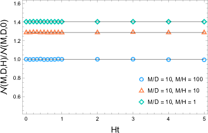
In general, we numerically find that $\langle z(t)\rangle$ matches the classical trajectory if $M\gg D\gg H$ (see fig. 1, right). If the value of the Hubble parameter $H$ is comparable with either the momentum variance $D$ or the scalar-field mass $M$ , then the wave-packet trajectory differs from the classical geodesic (59). Specifically, the initial wave-packet position deviates from $X=0$ if $H$ is non-negligible with respect to $D$ . Besides, the wave-packet propagation rate decreases with increasing $H$ and is negative if $H\sim M$ .

III.3.5 Wave-packet momentum in de-Sitter spacetime

The four-momentum of the classical particle can be directly found to read


$\displaystyle p^{t}(t)$	$\displaystyle=$	$\displaystyle\sqrt{M^{2}+e^{-2Ht}P^{2}}\,,$	(61a)
$\displaystyle p^{z}(t)$	$\displaystyle=$	$\displaystyle e^{-2Ht}P\,,$	(61b)

where $p^{x}(t)=p^{y}(t)=0$ due to the initial conditions considered and the spatial-translation symmetry of flat de-Sitter spacetime.

Making use of the commutator function in de-Sitter spacetime, one finds that the stress-tensor expectation value in the single-particle state $|\varphi_{X,P}\rangle$ is

	$\displaystyle\langle\hat{\Theta}_{\mu\nu}\rangle$	$\displaystyle=$	$\displaystyle\nabla_{\mu}\overline{\varphi}_{X,P}\nabla_{\nu}\varphi_{X,P}+\nabla_{\nu}\overline{\varphi}_{X,P}\nabla_{\mu}\varphi_{X,P}$		(62)
			$\displaystyle-\,\frac{1}{3}\,\nabla_{\mu}\nabla_{\nu}\|\varphi_{X,P}\|^{2}-\frac{1}{3}\,g_{\mu\nu}\big(\|\nabla\varphi_{X,P}\|^{2}-(M^{2}-H^{2})\|\varphi_{X,P}\|^{2}\big)\,,$		(62)

where we have omitted the vacuum contribution, as this does not depend on the wave packet. It is straightforward to show that this energy-momentum tensor is covariantly conserved, i.e. $\nabla^{\mu}\langle\hat{\Theta}_{\mu\nu}\rangle=0$ . Since $\{\partial_{i}\}$ are three Killing vectors of the de-Sitter universe, the momentum-conservation law holds, namely

\displaystyle\langle p_{i}(t)\rangle

\displaystyle\equiv

\displaystyle{\int_{\Sigma}}d\Sigma^{\mu}(x)\,\langle\hat{\Theta}_{i\mu}(x)\rangle\;=\;a^{3}(t){\int_{t}}d^{3}\mathbf{x}\,\langle\hat{\Theta}_{i}^{t}(x)\rangle

(63)

does not depend on the Cauchy surface $\Sigma$ (see fig. 2, left). Yet, the wave-packet energy,

\displaystyle\langle p_{t}(t)\rangle

\displaystyle\equiv

\displaystyle{\int_{\Sigma}}d\Sigma^{\mu}(x)\,\langle\hat{\Theta}_{t\mu}(x)\rangle\;=\;a^{3}(t){\int_{t}}d^{3}\mathbf{x}\,\langle\hat{\Theta}_{t}^{t}(x)\rangle

(64)

depends generically on cosmic time:

\displaystyle\frac{d}{dt}\,\langle p_{t}(t)\rangle

\displaystyle=

\displaystyle-H\langle p_{t}(t)\rangle+2M^{2}Ha^{3}(t){\int_{t}}d^{3}\mathbf{x}\,|\varphi_{X,P}(t,\mathbf{x})|^{2}\,,

(65)

where we have used $\nabla^{\mu}\langle\hat{\Theta}_{\mu\nu}\rangle=0$ and $\langle\hat{\Theta}_{\mu\nu}\rangle\rightarrow 0$ at spatial infinity (see fig. 2, right)

We numerically find that both $\langle p^{t}(t)\rangle$ and $\langle p^{z}(t)\rangle$ approach their classical values (61) if the condition $M\gg D\gg H$ is fulfilled, as shown in fig. 2. If otherwise, but still keeping $M\gg D$ , then the wave-packet energy $\langle p^{t}(t)\rangle$ increases as compared to $p^{t}(t)$ , whereas $\langle p^{z}(t)\rangle$ decreases in comparison to $p^{z}(t)$ . These observations seem to hint that $\langle p^{\mu}(t)\rangle$ is not a vector, meaning $\langle p^{\mu}(t)\rangle\langle p_{\mu}(t)\rangle$ might depend on a coordinate frame. We shall study this issue shortly.

The four-momentum $p^{\mu}(t)$ of the classical particle is proportional to its four-velocity $u^{\mu}(t)$ , namely $p^{\mu}(t)=Mu^{\mu}(t)$ . This formula follows from the energy-momentum tensor of a point-like particle whose mass density is given by the Dirac function Landau&Lifshitz. This relation implies that $\dot{z}^{z}(t)\equiv u^{z}(t)/u^{t}(t)=p^{z}(t)/p^{t}(t)$ , while, in quantum theory, one has

\displaystyle\langle\dot{z}(t)\rangle

\displaystyle=

\displaystyle+ie^{Ht}{\int_{t}}d^{3}\mathbf{x}\,\big(\varphi_{X,P}(x)\partial_{z}\overline{\varphi}_{X,P}(x)-\overline{\varphi}_{X,P}(x)\partial_{z}\varphi_{X,P}(x)\big)\,,

(66)

where we have taken into account that $\varphi_{X,P}(x)$ is a solution of the field equation (17), which tends to zero sufficiently fast at spatial infinity. This integral might now be expected to yield the classical result if $M\gg D\gg H\geq 0$ is fulfilled (see fig. 3).

III.3.6 Wave-packet position and momentum in co-moving frame

There is a coordinate frame in de-Sitter spacetime, in which the point-like particle moving along the geodesic (59) with $P\neq 0$ is at rest. This rest coordinate frame can be readily found by considering the de-Sitter-hyperboloid embedding into 5D Minkowski spacetime. Namely, the de-Sitter hyperboloid corresponds to the hypersurface $H^{2}\eta_{ab}\chi^{a}\chi^{b}=-1$ , where $\chi^{a}$ denote Minkowski coordinates, $\eta_{ab}$ stands for the Minkowski metric and the indices $a$ and $b$ run from $0$ to $4$ . Making use of (A12) in Anderson&Mottola, we obtain that the diffeomorphism to the rest frame of the point-like particle follows from the Lorentz transformation


$\displaystyle\chi^{0}$	$\displaystyle\rightarrow$	$\displaystyle\tilde{\chi}^{0}\;=\;\frac{\sqrt{M^{2}+P^{2}}}{M}\,\chi^{0}-\frac{P}{M}\,\chi^{3}\,,$	(67a)
$\displaystyle\chi^{1}$	$\displaystyle\rightarrow$	$\displaystyle\tilde{\chi}^{1}\;=\;\chi^{1}\,,$	(67b)
$\displaystyle\chi^{2}$	$\displaystyle\rightarrow$	$\displaystyle\tilde{\chi}^{2}\;=\;\chi^{2}\,,$	(67c)
$\displaystyle\chi^{3}$	$\displaystyle\rightarrow$	$\displaystyle\tilde{\chi}^{3}\;=\;\frac{\sqrt{M^{2}+P^{2}}}{M}\,\chi^{3}-\frac{P}{M}\,\chi^{0}\,,$	(67d)
$\displaystyle\chi^{4}$	$\displaystyle\rightarrow$	$\displaystyle\tilde{\chi}^{4}\;=\;\chi^{4}\,,$	(67e)

where $Ht=\ln{H(\chi^{0}+\chi^{4})}$ and $H\mathbf{x}=\boldsymbol{\chi}/(\chi^{0}+\chi^{4})$ . This coordinate transformation provides $t(\tau)\rightarrow\tau$ , $z(\tau)\rightarrow 0$ and $p(\tau)\rightarrow(M,0,0,0)$ , where $\tau$ is the proper time to parametrise points of the geodesic, $z(\tau)$ and $p(\tau)$ are, respectively, given in (59) and (61).

The initial conditions $X=0$ and $P=(\sqrt{M^{2}+P^{2}},0,0,P)$ turn, respectively, into $\tilde{X}=0$ and $\tilde{P}=(M,0,0,0)$ in the rest frame in which the covariant packet is spherically symmetric. In the absence of Lorentz-type deformations, its position expectation value coincides with the rest-frame origin. Furthermore, the wave-packet three-momentum also vanishes for the same reason. Hence, the covariant wave packet does not propagate in the rest frame, independent on relative values of the parameters $M>0$ , $D>0$ and $H\geq 0$ .

The rest-frame position of the packet can be computed from the non-rest-frame perspective and vice versa. In particular, we have

\displaystyle\langle\tilde{x}^{\mu}(\Sigma)\rangle

\displaystyle=

\displaystyle-i{\int_{\Sigma}}d\Sigma^{\nu}(x)\,\tilde{x}^{\mu}(x)\,\big(\varphi_{X,P}(x)\nabla_{\nu}\overline{\varphi}_{X,P}(x)-\overline{\varphi}_{X,P}(x)\nabla_{\nu}\varphi_{X,P}(x)\big)\,,

(68)

where $\tilde{x}^{\mu}=\tilde{x}^{\mu}(x)$ directly follows from (67). It is worth emphasising that $\langle\tilde{x}^{\mu}(\Sigma)\rangle$ depends on the Cauchy surface $\Sigma$ , rather than on $\tilde{\Sigma}$ . Still, one might expect that $\langle\tilde{x}^{\mu}(\Sigma)\rangle$ approximately coincides with $\langle\tilde{x}^{\mu}(\tilde{\Sigma})\rangle$ if the wave packet manifests itself as a classical particle.

Specifically, in the Minkowski-spacetime limit, i.e. $H\rightarrow 0$ , we have

\displaystyle\langle\tilde{z}(t)\rangle

\displaystyle\xrightarrow[H\,\rightarrow\,0]{}

\displaystyle\frac{\sqrt{M^{2}+P^{2}}}{M}\,\langle z(t)\rangle-\frac{P}{M}\,t\,,

(69)

which vanishes if and only if $\langle z(t)\rangle=z(t)$ . This equality approximately holds iff $M\gg D$ , as shown in Sec. III.2.2. Now, if we assume $H>0$ , then $\langle\tilde{z}(t)\rangle$ can be expected to approach zero if the packet propagates along the classical geodesic (59), i.e. $M\gg D\gg H$ must be satisfied. If otherwise, $\langle\tilde{z}(t)\rangle$ may be non-vanishing. This discrepancy is illustrated on fig. 4, left.¹¹ 1 The integrand in (68) turns out to be singular at $x=y=0$ and $z=(P/(\sqrt{M^{2}+P^{2}}-M)\pm\exp(-Ht))/H$ for all $Ht\geq 0$ . This singularity originates from the scale factor $\exp(H\tilde{t})$ which, if expressed through $t$ and $\mathbf{x}$ by using (67), vanishes at those points. Therefore, the expectation value of $\tilde{\chi}^{3}(t,\mathbf{x})=\tilde{z}(t,\mathbf{x})\exp(H\tilde{t}(t,\mathbf{x}))$ instead of $\tilde{z}(t,\mathbf{x})$ is shown in that figure. This problem is non-existent if those points lie outside the wave-packet support, e.g., if $P/M=1$ , that is the case for a packet whose support is inside the Hubble volume.

The rest-frame four-momentum of the wave packet can also be calculated from the non-rest-frame perspective:

\displaystyle\langle\tilde{p}_{\mu}(\Sigma)\rangle

\displaystyle=

\displaystyle{\int_{\Sigma}}d\tilde{\Sigma}^{\nu}(\tilde{x})\,\langle\tilde{\Theta}_{\mu\nu}(\tilde{x})\rangle\;=\;{\int_{\Sigma}}d\Sigma^{\rho}(x)\,\frac{\partial x^{\lambda}}{\partial\tilde{x}^{\mu}}\,\langle\Theta_{\lambda\rho}(x)\rangle\,,

(70)

where $\langle\hat{\Theta}_{\mu\nu}(x)\rangle$ is a second-rank tensor, because $\varphi_{X,P}(x)$ is a relativistic scalar. In Minkowski spacetime, $\langle\tilde{p}_{\mu}(\Sigma)\rangle$ coincides with $\langle\tilde{p}_{\mu}(\tilde{\Sigma})\rangle$ in the absence of external forces. This happens to be the case, since the four-momentum is then independent on Cauchy surfaces. In de-Sitter spacetime, their coincidence might be expected if $M\gg D\gg H$ holds (see fig. 4, right).

To summarise, the non-rest- and rest-frame computations of the position and momentum expectation values are related like in classical physics if the wave packet behaves as a point-like particle. According to the numerical calculations, this requires the Compton wavelength to be much smaller than the wave-packet localisation size which, in turn, must be negligibly small relative to the curvature length. The former is needed for the suppression of quantum features of the packet, while the later for it to be oblivious to the global geometry.

IV Discussion

Elementary particles are described by wave packets in quantum theory. A wave packet in Minkowski spacetime is usually constructed through the superposition of positive-frequency plane-wave solutions of a given field equation Itzykson&Zuber. This wave packet can in turn be associated with an asymptotic state used in the definition of $S$ -matrix. But, the plane-wave solutions may exist only locally in non-flat spacetimes. The basic question is then how to construct a wave packet to describe a free elementary particle in the Universe.

In flat de-Sitter spacetime, one believes that the exact solution (5a) is appropriate for the definition of elementary particles at past infinity, while the solution (5b) is usually suggested for the description of particles at future infinity. The superposition of each of these modes can certainly be used to construct Gaussian wave packets. The three-momentum of these packets are given by the Minkowski result (30b). Hence, we should assume $M\gg D$ for each packet. In addition, we should assume $D\gg H$ , otherwise these wave packets have spatial support to be larger than the cosmological extent of de-Sitter spacetime. In general, any wave packet should be well localised within the Hubble scale in order to describe an elementary particle. Repeating numerical calculations made in the previous sections, we find these two Gaussian wave packets propagate along a curve which approaches the geodesic (59) if $M\gg D\gtrsim H$ . In this case, the energy of the packets also approaches the classical result (61a).

Still, the adiabatic wave packets cannot be locally represented through the superposition of plane waves and depend on coordinates used to parametrise the de-Sitter hyperboloid. All these mean that the adiabatic wave packets are locally described by phase factors which may differ from $e^{-iM\tau}$ , where $\tau$ is the proper time. In particular, their on-mass-shell phase factors depend explicitly on the three-momentum. Specifically, taking the same initial conditions as in the previous section, we find that that difference becomes more pronounced if we increase the ratio $P/M$ for fixed $M/D=10$ and $M/H=100$ . In fact, expressing $t$ and $z$ through the proper time $\tau$ and then considering $H\tau\ll 1$ , we obtain


$\displaystyle a(t(\tau))$	$\displaystyle\approx$	$\displaystyle 1+\sqrt{1+\frac{P^{2}}{M^{2}}}\,H\tau\,,$	(71a)
$\displaystyle z(\tau)$	$\displaystyle\approx$	$\displaystyle\frac{P}{M}\,\frac{\tau}{a(t(\tau))}\,.$	(71b)

The adiabatic-wave-packets phase factors do reduce to $e^{-iM\tau}$ iff $M/H\gg 1$ and $P/M\lesssim 1$ . This is no longer the case if $P/M\gg 1$ and $PH\tau/M\gtrsim 1$ hold. If we now assume that $\tau\sim 1\,\text{s}$ , $H=H_{0}\sim 10^{-18}\,\text{s}^{-1}$ and $M\sim 1\,\text{MeV}$ , then the discrepancy should appear for $P\gtrsim 10^{15}\,\text{GeV}$ . This result turns out to be counter-intuitive, because high-energy physics should not depend on the space-time curvature. This property of the adiabatic wave packets might thereby lead to non-standard results for flavour oscillations and for the quantum interference induced by gravity. However, $H_{0}$ is way too small for any experimental tests of that and, moreover, the observable Universe can be modelled by de-Sitter spacetime at cosmological scales only. It means this issue should be studied in Schwarzschild spacetime which approximately describes the local geometry of Earth (see below for more details on this point).

The main purpose of this article was to derive a wave packet which is a relativistic scalar and locally reduces to the plane-wave superposition at any space-time point, no matter if that point lies at past or future cosmic infinity or somewhere in between. These basic properties are required for a wave packet to be appropriate for the description of an elementary particle. In particle physics, the Minkowski-spacetime approximation of the Universe is underlying for the definition of particles which are related to the unitary and irreducible representations of the Minkowski-spacetime isometry group Weinberg. Thus, those properties guarantee that the wave packet locally corresponds to the irreducible representation of mass $M$ and spin $0$ . The main result of the article is that we have found that such a packet does exist in de-Sitter spacetime. This packet propagates over cosmological times like a point-like particle of the same mass if $M\gg D\gg H$ (see also fig. 5), such that the wave-packet phase is characterised by $e^{-iM\tau}$ , as expected in the semi-classical limit Stodolsky. If otherwise, it propagates highly non-classically.

This wave-packet solution, $\varphi_{X,P}(x)$ , gives rise to the particle-annihilation operator

\displaystyle\hat{a}(\varphi_{X,P})

\displaystyle=

\displaystyle+i{\int_{\Sigma}}d\Sigma^{\mu}(x)\,\big(\overline{\varphi}_{X,P}(x)\nabla_{\mu}\hat{\Phi}(x)-\hat{\Phi}(x)\nabla_{\mu}\overline{\varphi}_{X,P}(x)\big)\,.

(72)

This operator has two basic properties, namely it does not depend on the Cauchy surface $\Sigma$ and on the coordinates $x$ used to parametrise the de-Sitter hyperboloid. The former property comes from, first, the absence of non-linear terms in the scalar-field equation and, second, the localisation of $\varphi_{X,P}(x)$ on the Cauchy surface $\Sigma$ . The latter property is due to the covariant character of the Klein-Gordon product and the wave-packet solution $\varphi_{X,P}(x)$ . Thus, $\hat{a}(\varphi_{X,P})$ defines a coordinate-independent quantum vacuum ( $\hat{a}(\varphi_{X,P})|\Omega\rangle=0$ ) in de-Sitter spacetime, while its Hermitian conjugate defines a covariant particle state ( $|\varphi_{X,P}\rangle=\hat{a}^{\dagger}(\varphi_{X,P})|\Omega\rangle$ ).

The quantum state $|\Omega\rangle$ is a no-covariant-particle state which still may be non-empty with respect to the de-Sitter particles which have been introduced in Sec. II. To clarify this issue, the Bogolyubov coefficients need to be computed:


$\displaystyle\alpha_{X,P}(\mathbf{k})$	$\displaystyle\equiv$	$\displaystyle-ie^{3Ht}{\int_{t}}d^{3}\mathbf{x}\,\big(\varphi_{X,P}(x)\partial_{t}\bar{\varphi}_{\mathbf{k},-\infty}(x)-\bar{\varphi}_{\mathbf{k},-\infty}(x)\partial_{t}\varphi_{X,P}(x)\big)\,,$	(73a)
$\displaystyle\beta_{X,P}(\mathbf{k})$	$\displaystyle\equiv$	$\displaystyle-ie^{3Ht}{\int_{t}}d^{3}\mathbf{x}\,\big(\bar{\varphi}_{X,P}(x)\partial_{t}\bar{\varphi}_{\mathbf{k},-\infty}(x)-\bar{\varphi}_{\mathbf{k},-\infty}(x)\partial_{t}\bar{\varphi}_{X,P}(x)\big)\,,$	(73b)

which are time-independent due to the spatial localisation of $\varphi_{X,P}(x)$ . Having used the same initial conditions for $X$ and $P$ as in the previous section, we numerically find for $\mathbf{k}=\mathbf{P}$ that $\alpha_{X,P}(\mathbf{k})$ is time-independent, while $\beta_{X,P}(\mathbf{k})$ fluctuates with time and $|\beta_{X,P}(\mathbf{k})/\alpha_{X,P}(\mathbf{k})|\lll 1$ decreases if an integration region increases. The same calculations with $\varphi_{\mathbf{k},-\infty}(x)$ replaced by $\varphi_{\mathbf{k},+\infty}(x)$ yield the Bogolyubov coefficients which are time-independent. These observations might mean that $|\Omega\rangle$ is unitarily equivalent to the state $|\text{dS}\rangle$ . In any case, $\varphi_{X,P}(x)$ is related to the 2-point function in the de-Sitter state, as shown in Sec. III.3.2. Specifically, $\varphi_{X,P}(x)$ is proportional to that function if $D\rightarrow\infty$ . This turns out to be analogous to the Minkowski case, namely the packet (26) is also proportional to the Minkowski 2-point function if the momentum variance of the wave packet is infinite. In both cases, the proportionality coefficient is given by the normalisation factor.

The de-Sitter universe is not only one curved spacetime which is of physical interest from the viewpoint of elementary particle physics. For example, black-hole spacetimes serve as a non-trivial background for probing predictions of quantum theory. Field-equation solutions which are commonly employed to define particles depend explicitly on global symmetries of a given black-hole geometry DeWitt-1975. Still, the observable Universe can locally be approximated by such a geometry only nearby a black hole this geometry is supposed to describe. Thereby, black-hole global symmetries are local for the Universe. This circumstance poses a question why those global symmetries should be “preferred” with respect to local Poincaré symmetry, taking into account that both are non-exact in the Universe. Since local Poincaré symmetry is well known to play a crucial role in elementary particle physics Weinberg, one might actually need to re-consider those solutions which are employed to define elementary particles in black-hole spacetimes. The reason is that those solutions like $\varphi_{\mathbf{k},-\infty}(x)$ and $\varphi_{\mathbf{k},+\infty}(x)$ give rise to wave packets which cannot be everywhere represented locally through the superposition of plane waves, as required by the equivalence principle and collider physics. This might lead to novel results in quantum-black-hole physics, such as Emelyanov.

This question does not seem to be unanswerable nearby Earth, because its local curvature length is around $10^{11}\,\text{m}$ , which is 15 orders of magnitude smaller than that of the observable Universe as a whole. This would naively reduce the threshold momentum to around $1\,\text{GeV}$ , above which the standard mode solutions in Schwarzschild spacetime may lead to the local-Lorentz-symmetry violation under certain experimental conditions. We shall report on this study in one of our future publications.

ACKNOWLEDGMENTS

It is my pleasure to thank Prof. O. Nachtmann for providing the reference Nachtmann1968. I am also grateful to Martin Gabelmann for his support by working with the ITP computer cluster.

References

(1) E. Schrödinger, Physica 6 (1939) 899.
(2) L. Parker, Phys. Rev. 183 (1969) 1057.
(3) L. Parker, D. Toms, Quantum Field Theory in Curved Spacetime. Quantized Fields and Gravity (Cambridge University Press, 2009).
(4) S. Weinberg, Quantum Theory of Fields (Cambridge University Press, 1995).
(5) W. Pauli, Zur älteren und neueren Geschichte des Neutrinos, in Aufsätze und Vorträge über Physik und Erkenntnistheorie (Friedr. Vieweg & Sohn, Braunschweig, 1961).
(6) C.M. Will, Living Rev. Relativ. 9 (2006) 3.
(7) R. Colella, A.W. Overhauser, S.A. Werner, Phys. Rev. Lett. 34 (1975) 1472.
(8) L. Stodolsky, Gen. Rel. Grav. 11 (1979) 391.
(9) P.R. Anderson, E. Mottola, Phys. Rev. D 89 (2014) 104038.
(10) P.R. Anderson, E. Mottola, D.H. Sanders, Phys. Rev. D 97 (2018) 065016.
(11) N.A. Chernikov, E.A. Tagirov, Ann. Inst. H. Poincaré A 9 (1968) 109.
(12) T.S. Bunch, P.C.W. Davies, Proc. R. Soc. A 360 (1978) 117.
(13) O. Nachtmann, Commun. Math. Phys. 6 (1967) 1.
(14) O. Nachtmann, Österr. Akad. Wiss., Math.-Naturw. Kl., Abt. II 176 (1968) 363.
(15) J. Bros, H. Epstein, U. Moschella, JCAP 02 (2008) 003; Ann. Henri Poincaré 11 (2010) 611.
(16) C.W. Misner, K.S. Thorne, J.A. Wheeler, Gravitation (W.H. Freeman and Co., 1973).
(17) V.F. Mukhanov, Physical Foundations of Cosmology (Cambridge University Press, 2005).
(18) E. Merzbacher, Quantum Mechanics (3rd Edition, John Wiley & Sons, Inc., 1998).
(19) C. Itzykson, J.-B. Zuber, Quantum Field Theory (McGraw-Hill Inc., 1980).
(20) D.V. Naumov, V.A. Naumov, J. Phys. G: Nucl. Part. Phys. 37 (2010) 105015.
(21) D.V. Naumov, Phys. Part. Nuclei Lett. 10 (2013) 642.
(22) H. Lehmann, K. Symanzik, W. Zimmermann, Nuovo Cimento 1 (1955) 205.
(23) T.D. Newton, E.P. Wigner, Rev. Mod. Phys. 21 (1949) 400.
(24) B.S. DeWitt, Dynamical Theory of Groups and Fields (Gordon and Breach, 1965).
(25) I.S. Gradshteyn, I.M. Ryzhik, Tables of Integrals, Series, and Products (7th Edition, Elsevier Inc., 2007).
(26) F.W.J. Olver, D.W. Lozier, R.F. Boisvert, C.W. Clark, NIST Handbook of Mathematical Functions (Cambridge University Press, 2010).
(27) A.M. Polyakov, Nucl. Phys. B 797 (2008) 199; Nucl. Phys. B 834 (2010) 316.
(28) C.B. Balogh, Bull. Amer. Math. Soc. 72 (1966) 40; SIAM J. Appl. Math. 15 (1967) 1315.
(29) W. Magnus, F. Oberhettinger, R.P. Soni, Formulas and Theorems for the Special Functions of Mathematical Physics (3rd Edition, Springer-Verlag, 1966).
(30) L.D. Landau, E.M. Lifshitz, The Classical Theory of Fields. Course of Theoretical Physics. Volume 2. (4th Edition, Butterworth-Heinemann, 1980).
(31) B.S. DeWitt, Phys. Rep. 19 (1975) 295.
(32) V.A. Emelyanov, Fortsch. Phys. 67 (2019) 1800114; Class. Quant. Grav. 36 (2019) 075018.