Towards analyzing large graphs with quantum annealing and quantum gate computers

As we see in the following, finding the $\min L$ in a bipartite graph can be seen also as a basic operation in finding communities in a graph. We consider the case when the graph has communities generated from a stochastic block model (SBM), for a review see [2].

SBM($n,k,P,D$) is a generative probabilistic graph model defined as follows. Here $P$ is a probability distribution on $[k]=\{1,\dots,k\}$ and $D$ is a symmetric $k$-by-$k$ matrix with entries $D_{i,j}\in[0,1]$. The model is generated by first sampling node labels $\sigma(1),\dots,\sigma(n)$ independently from $P$, and then creating a random graph on node the set $V$ by linking each unordered node pair $\{u,v\}$ with probability $D_{\sigma(u),\sigma(v)}$, independently of other node pairs. The node labeling $\sigma:V\to[k]$ partitions the node set into $k$ disjoint communities $V_{i}=\sigma^{-1}(i)$, so that

Conditionally on the node labeling $\sigma$, the nodes between communities $V_{i}$ and $V_{j}$ are hence linked with probability $D_{i,j}$. The resulting random graph is denoted as $\mathcal{G}(n,k,P,D)$.

In our previous works, we have extensively referred to SRL as a basis for graph analysis using various SBMs as a modeling space [1, 5, 6, 7, 8, 9]. Here we introduce another contact point between SBM and SRL.

Assume that a graph $G$ is drawn from $\mathcal{G}(n,k,P,D)$ as described above. We also assume that $n$ is large enough.

The first step is to find a bipartite subgraph, $G^{\prime}$ of $G$:

• •

  divide nodes of $G$ into two disjoint sets $A$ and $B$, by tossing a fair coin for each node

• •

  $G^{\prime}$ inherits all links from $G$ that join $A$ and $B$ while all links inside $A$ and $B$ are deleted.

This procedure is schematically shown in Fig. 2

We denote: $A_{i}:=A\cap V_{i}$ and $B_{i}:=B\cap V_{i}$ with sizes $a_{i}:=\absolutevalue{A_i}$ and $b_{i}:=\absolutevalue{B_i}$ for $i=1,\cdots,k$. It is clear that random variables $(a_{1},\cdots,a_{k},b_{1},\cdots,b_{k})$ have a multinomial distribution with expectations $\mathbb{E}a_{i}=\mathbb{E}b_{i}=nP_{i}/2$ for all $i$. For large $n$ these random variables are well concentrated around their expected values.

Denote by $d$ the link density of bipartite graph: $d=e(A,B)/(\absolutevalue{A}\absolutevalue{B})$. For a large graph, $d$ is close to the expected link density of the original graph $G$, $d(G)$, with high probability. We require the following

This inequality means that all communities have internal density above the average density. For large graphs, we also have with high probability:

It is required that the Condition 4 holds when $G$ is replaced by a subgraph of $G$ in which arbitrary communities are deleted.

We do not provide a lengthy proof of the last claim. Typically probabilistic estimates are exponential, so this statement has high probability already with moderate graph sizes.

The idea behind community detection is the following. If there are bigger densities of links inside the communities than those between the communities, then the communities in the split graph are associated with the denser parts of the corresponding bipartite graph. As a result, there is a chance that communities can be found with the help of $\argmin L$ applied to the split graph.

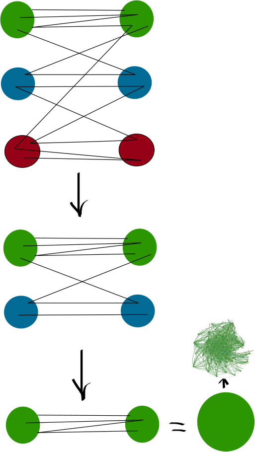
The next step of the algorithm is to construct the $L$-function for the bipartite graph of the split communities described above. The output of the algorithm is the subgraph induced by $\argmin L$. The algorithm works correctly if the following conjecture is true:

We do not possess a full proof of this claim. As a first sketch, we consider optimization of expected $L$-function conditional to the sizes of split communities. The basic setting is the same as in Conjecture 1. We denote $x_{i}=\absolutevalue{X \cap A_i}$ and $y_{i}=\absolutevalue{Y \cap B_i}$. These integers are bounded by $0\leq x_{i}\leq a_{i}$ and $0\leq y_{i}\leq b_{i}$. In shorthand, we write $x\in[0,a]$ and $y\in[0,b]$ and recall that such constraints are usually referred as box constraints [12]. In these notations, we have:

Let us condition with respect to $a_{1},\cdots,a_{k},b_{1},\cdots b_{k}$ and take the expectation of $L$ over the SBM:

in which $d$ is the expected link density of the bipartite graph conditionally on the underlying community structure. We assume that we are in the high-probability event when the Condition 4 holds.

To prove Conjecture 1, we need some probability concentration inequalities like Chernoff bounds for known distributions with which we are dealing. The martingale argument may be used as was shown in an analogous case [11]. Proposition 2 shows that the Conjecture holds on average and provides a starting point for the proof. Then one should use concentration inequalities of probability theory to show that the solution of stochastic problem is the same with high probability.

After the first step, the algorithm proceeds similarly on the found subgraph corresponding to $\argmin L$. It runs until only one community is left. Then the found community is deleted from $G$ and the whole process is repeated until all communities are found, see Fig 3.

D-Wave Systems Inc. has published a quantum computing cloud service, Leap [13], for free trial and an option for buying quantum processing time. The Leap provides immediate access to a D-Wave 2000Q quantum computer or annealer. The computer has up to $2048$ qubits and the service provides support for users such as the demos, interactive learning material and the Ocean software development kit (SDK) with suite of open-source Python tools and templates.

When one has a qubo (2) in the form of (3), it is quite straightforward to implement and run it on the quantum computer. The size of the problem is restricted by the connectivity between qubits in the D-wave 2000Q Chimera architecture and the number of qubits available.

For an arbitrary problem (2) an embedding is needed and that can drastically reduce the size of the problem that can be solved. For large problems, a hybrid approach is suggested, in which the problem is split into smaller pieces and part of the computations are done classically, so-called qbsolver. The Ocean SDK provides functions for automatic embedding as well as for solving a large qubo by qbsolver. D-Wave has announced that the next generation version of the quantum computer with over $5000$ qubits and added connectivity between qubits would be available in mid-2020.

D-Wave quantum computer uses large number of quantum bits or qbits. In this section our aim is to verify connection between quadratic optimization and the ground state of the corresponding quantum system in D-wave machine. We also review some basic concepts of quantum computation theory needed for this purpose. One qbit, a quantum version of a bit or a binary variable is described by a vector $\ket{Z}\in\mathbb{C}^{2}$, which is the complex vector space of dimension 2. $\ket{Z}$ are referred as ket-vectors.

Elements of dual vector space are called bra-vectors and are denoted as $\bra{Z}\in\mathbb{C}^{2*}$, which forms a complex vector space of dimension 2

$\mathbb{C}^{2*}$ is just space of all row vectors with two complex coordinates: $(z_{1},z_{0})$

Notations:

where, $T$ stands for matrix transposition.

Any vector in $\mathbb{C}^{2}$ or $\mathbb{C}^{2*}$ can be written: $Z:=\ket{Z}=z_{1}\ket{1}+z_{0}\ket{0}$, $\bra{Z}=\ket{Z}^{\dagger}=\bra{1}z_{1}^{*}+\bra{0}z_{0}^{*}$, where $\dagger$ stands for transposition and complex conjugate (Hermite transpose). Inner product is understood as a matrix multiplication:

where we used orthogonality conditions $\bra{i}\ket{j}=\delta_{i,j}$, with $i,j\in\{0,1\}$ and $\delta_{i,j}=1$ if $i=j$ and zero otherwise. These conditions follow directly from our definitions.

Classical register of length $n$ is a tuple of binary variables: $R=(b_{1},b_{2},\cdots,b_{n})$, $b_{i}\in\{0,1\}$

Quantum register of length $n$ is a system of $n$ qbits. As in one qbit case, states in which all qbits have some particular value form a basis and are denoted as:

We assume that the carriers of qbit states are not identical entities, which is usually the case. In the opposite case the state vectors would have additional bosonic or fermionic symmetry property upon permutations.

If $n$ qbits are in any state $\ket{R}$ result of measuring of qbits is always register $R$. Such states we call the product states. Qbits can be in any linear combination of such product states with arbitrary complex numbers, which add up to on in square modules, as coefficients:

State space of quantum register with $n$ qbits ($H_{n}$) is called tensor product of n spaces $\mathbb{C}^{2}$:

Defining the inner product in $H_{n}$ as:

$H_{n}$ is turned into a Hilbert space of dimension $2^{n}$.

The interpretation of quantum register state is probabilistic. When qbits are measured, probability of an outcome $(b_{1},\cdots,b_{n})$ in state $\ket{\Psi}$ is:

A general state in $H_{n}$ is called entangled state. An entangled state is a superposition of product states. The product states, where each qbit has a definite state, is only a tiny fraction of the $H_{n}$:

Take $n=333$, then a state of $H_{n}$ is described by more than $10^{100}$ real parameters. Such a manifold is impossible to ’digitize’, at least in our universe!

Operators in $n$-qbit Hilbert space, $H_{n}=(\mathbb{C}^{2})^{\otimes n}$, are in general $2^{n}\times 2^{n}$ matrices. One way of defining such operators is a tensor product of operators. Let $X_{1}$ and $X_{2}$ be operators acting in space of the first - and the second qbit. The tensor product of these operators acts on product states according to rule:

The $X_{1}\otimes X_{2}$ is defined in the whole $H_{2}$ by linearity. Generalization to a case of arbitrary number of factors $n$ is done similarly.

Quantum annealing system in D-Wave architecture has Hamiltonian:

in which $\sigma_{zi}$ is a Pauli matrix $\sigma_{z}$ acting on qbit $i$, $h_{i}$ and $J_{i,j}$ are adjustable real parameters. This is a short hand notation, unit matrix $I$ is assumed in the tensor product not occupied by $\sigma_{z}$, for instance $h_{1}\sigma_{z1}=h_{1}\sigma_{z1}\otimes I_{2}\otimes\cdots\otimes I_{n}$ and so on.

Corollary: Ground-state of the D-Wave system corresponds to $\min E_{I}$. Eigenstates are product states - no entanglement.

The regularity check (RC) of a bipartite graph is computationally hard problem requiring, in the worst cases, exponential time in number of nodes. Quantum search using so called Grover’s algorithm (see e.g. [19]) could improve the time needed for the RC. The time is still exponential but with smaller base of the exponential function. This corresponds to the famous speed-up from $N$ to $\sqrt{N}$, corresponding to exhaustive search of $N$ items with classical versus Grover’s search.

Grover’s algorithms finds solution to the following problem: let among $N=2^{m}$ items, encoded as integers $M:=\{0,\cdots,N-1\}$, be exactly one marked element $x_{0}\in M$; find $x_{0}$. It is assumed that there is a function $f:M\rightarrow\{0,1\}$ such that $f(x_{0})=1$ and otherwise $f(x)=0$ for all other $x\in M$. It is assumed that $f$ can be computed quickly. In other words if the solution is found, it can be easily verified as such.

First step is to map items to a register of $m$ qbits. Each number $x\in M$ is written as a binary tuple of $m$ bits: $(x_{1},\cdots,x_{m})$, $x_{i}\in\{0,1\}$. Then such a number is mapped to the quantum state of $m$ qbits: $\ket{x}=\ket{x_1\cdots x_m}$.

The quantum oracle is an unitary operator acting according to the rule: $R_{f}\ket{x_0}=-\ket{x_0}$ and $R_{f}\ket{x}=\ket{x}$, $\forall x\neq x_{0}$. Superposition of all states corresponding to $M$ is denoted as $\ket{D}=\frac{1}{\sqrt{N}}\sum_{x\in M}\ket{x}$. $R_{D}:=2\ket{D}\bra{D}-I$ is another unitary operator needed. Product of these two operators is unitary operator $U:=R_{D}R_{f}$, which is the main transformation in Grover’s algorithm. The process starts from state $\ket{D}$; after $t\in\mathbb{N}$ steps the system is in the state:

If $t_{0}=\left\lfloor\frac{\pi}{4}\sqrt{N}\right\rfloor$, then with probability $p_{0}>1-\frac{1}{N}$, the state $\ket{\psi_{t_0}}$ is $\ket{x_0}$, and the binary representation of the solution $x_{0}$ is found by measuring the state of the quantum register $\ket{\psi_{t_0}}$.

An analysis shows that $U^{t}\ket{D}$ is a rotation by an angle $t\theta$ in two dimensional plane spanned by vectors $\ket{x_0}$ and $\ket{D}$ in which $\theta\approx\frac{2}{\sqrt{N}}$ is a constant. In this plane $U$ has representation:

Eigenvalues of this matrix are $e^{i\theta}$ and $e^{-i\theta}$. The corresponding eigenvectors are:

in which $\ket{1}$ corresponds to the state $\ket{x_0}$ and $\ket{0}$ corresponds to the vector orthogonal to $\ket{x_0}$ in the two dimensional plane we described above. In these notations the initial vector $\ket{D}$ can be written as:

As a result we have:

which indicates that square of amplitude of the $\ket{1}$, which is $\sin^{2}(\theta t+\frac{\theta}{2})$, at step $t=t_{0}$ is very close to one. This means that when the register is read/measured, the result is $\ket{x_0}$ with probability very close to one, assuming large $N$. This also indicates that $t_{0}$ should be known. For $t>t_{0}$, the amplitude of $\ket{x_0}$ starts to decrease.

In case there are $\absolutevalue{M}\geq 1$ solutions to equation $f(x)=1$, similar algorithm works. However, the $\theta$-parameter changes to $\theta=2\sqrt{\frac{\absolutevalue{M}}{N}}$, and similarly number of steps changes. As a result, in order to use Grover’s algorithm, the number of solutions need to be known beforehand. For details, see e.g. [19].

It appears that there exist quantum algorithms for evaluating number of solutions without actually finding the solutions, [21]. One of them is based on estimating eigenvalue of an unitary operator, which is of the form $e^{i\theta}$, $\theta\in[0,2\pi)$. Indeed if we can find eigenvalue of $U$ of the Grovers’s operator: $U\ket{\alpha_1}=e^{i\theta}\ket{\alpha_1}$, we can find out number of solutions, since $\theta=2\sqrt{\frac{\absolutevalue{M}}{N}}$. This covers the case in which there is no solution: $U=I$, and $\theta=0$. This problem is called quantum phase estimation problem. The task of finding out whether $\absolutevalue{M}=0$ or $\absolutevalue{M}>0$, is called quantum existence problem [21].

Quantum phase estimation, see [20], is based on quantum Fourier transformation ($QFT$). $QFT$ is a linear mapping between $m$ qbit states:

the inverse mapping is:

For any superposition of states $QFT$ and $QFT^{-1}$ are defined by linearity, say, $QFT(\sum_{i}c_{i}\ket{i})=\sum_{i}c_{i}QFT(\ket{i})$.

In case of $m$ qbits we have integers $a:0\leq a\leq 2^{m-1}$, and we can write $a$ in binary basis: $a=2^{m-1}a_{m}+2^{m-1}a_{2}+\cdots+2^{0}a_{1}$, where coefficients $a_{i}$ are binary numbers. Then, by definition, we write:

It appears that $QFT$ can be written as:

Let assume that unitary operator $U$ has eigenstate $\ket{u}$, with eigenvalue $e^{i\theta}=e^{2\pi i0.a_{m}a_{m-1}\cdots a_{1}}$ ( $m$-binary-digit eigenvalue).

An operator $C\_U$, called the controlled $U$. It acts on vectors like $\frac{1}{\sqrt{2}}(\ket{0}+\ket{1})\otimes\ket{u}$. $C\_U$ acts as $U$ on the $\ket{u}$ if the value of the first qbit is 1, otherwise it is unit operator, for instance:

The phase estimation uses the following scheme. First register has $m$ qbits, all in states $\frac{1}{\sqrt{2}}(\ket{0}+\ket{1})$, second register is in the state $\ket{u}$, the eigenstate of $U$, phase of which we wish to find. Then controlled $U$ operators are applied in sequence: $C_{j}\_U^{2^{j}}$, $j=0,1,\cdots,m-1$, where controlled $U$ with index $j$, uses $j$th qbit from the bottom of the first register as a control qbit. It easy to check that the state of the register after these operations equals to (omitting the normalization coefficient):

References

- [1] H. Reittu, I. Norros and F. Bazsó, Regular decomposition of large graphs and other structures: scalability and robustness towards missing data, In Proc. Fourth International Workshop on High Performance Big Graph Data Management, Analysis, and Mining (BigGraphs 2017), Eds. M. Al Hasan, K. Madduri and N. Ahmed, Boston U.S.A., 2017
- [2] Abbe, E.: Community detection and stochastic block models: recent developments, arXiv:1703.10146v1 [math.PR] 29 Mar 2017
- [3] Szemerédi, E.: Regular Partitions of graphs. Problemés Combinatories et Téorie des Graphes, number 260 in Colloq. Intern. C.N.R.S.. 399-401, Orsay, 1976
- [4] Fox, J., Lovász, L.M., Zhao, Yu.: On regularity lemmas and their algorithmic applications. arXiv:1604.00733v3[math.CO] 28. Mar 2017
- [5] Nepusz, T., Négyessy, L., Tusnády, G., Bazsó, F.: Reconstructing cortical networks: case of directed graphs with high level of reciprocity. In B. Bollobás, and D. Miklós, editors, Handbook of Large-Scale Random Networks, Number 18 in Bolyai Society of Mathematical Sciences pp. 325 – 368, Spriger, 2008
- [6] Pehkonen, V., Reittu, H.: Szemerédi-type clustering of peer-to-peer streaming system. In Proceedings of Cnet 2011, San Francisco, U.S.A. 2011
- [7] Reittu, H., Bazsó, F., Weiss, R.: Regular decomposition of multivariate time series and other matrices. In P. Fränti and G. Brown, M. Loog, F. Escolano, and M. Pelillo, editors, Proc. S+SSPR 2014, number 8621 in LNCS, pp. 424 – 433, Springer 2014
- [8] Reittu, H., Bazsó, F., Norros, I. : Regular Decomposition: an information and graph theoretic approach to stochastic block models arXiv:1704.07114[cs.IT], 2017
- [9] Hannu Reittu, Lasse Leskelä, Tomi Räty, Marco Fiorucci, Analysis of large sparse graphs using regular decomposition of graph distance matrices, In Proc. IEEE BigData 2018, Seattle U.S.A., pp. 3783-3791, Workshop: Advances in High Dimensional (AdHD) Big Data, Ed. Sotiris Tasoulis.
- [10] Terence Tao, Szemerédi’s regularity lemma revisited, January 2006, Contributions to Discrete Mathematics 1(1).
- [11] Hannu Reittu, Ilkka Norros, Tomi Räty, Marianna Bolla, Fülöp Bazsó, Regular decomposition of large graphs: foundation of a sampling approach to stochastic block model fitting Hannu Reittu, Data Sci. Eng. (2019) 4: 44-60. https://doi.org/10.1007/s41019-019-0084-x
- [12] Floudas C.A., Visweswaran V. (1995) Quadratic Optimization. In: Horst R., Pardalos P.M. (eds) Handbook of Global Optimization. Nonconvex Optimization and Its Applications, vol 2. Springer, Boston, MA
- [13] https://www.dwavesys.com/take-leap
- [14] Sanjeeb Dash, A note on QUBO instances defined on Chimera graphs, arXiv:1306.1202 [math.OC], 2013
- [15] C. C. McGeoch, C. Wang (2013) Experimental Evaluation of an adiabatic quantum system for combinatorial optimization. Proceedings of the 2013 ACM Conference on Computing Frontiers 2013, Ischia, Italy.
- [16] Ch. F. A. Negre, H. Ushijima-Mwesigwa, S. M. Mniszewski, Detecting Multiple Communities Using Quantum Annealing on the D-Wave System, arXiv:1901.09756 [cs.OH], 2019
- [17] https://www.fz-juelich.de
- [18] https://github.com/hannureittu/Community-panning/blob/master/AdevelopeKoe.py
- [19] R. Portugal, Quantum Walks and Search Algorithms, Springer, 2018
- [20] R. Cleve, A. Ekert, C. Macchiavella, M.Mosca, Quantum Algorithms Revisited, Proc. R. Soc., London A, pp. 339-354, 1998
- [21] S. Imre, Quantum Existence Testing and Its Application for Finding Extreme Values in Unsorted Databases, IEEE Trans. Computers, Vol 56, No.5,pp. 706-710, 2007