Femtoscopy scales and particle production in the relativistic heavy ion collisions from Au+Au at 200 AGeV to Xe+Xe at 5.44 ATeV within the integrated hydrokinetic model
Abstract
The recent results on the main soft observables, including hadron and photon yields and particle number ratios, spectra, flow harmonics, as well as the femtoscopy radii, obtained within the integrated hydrokinetic model (iHKM) for high-energy heavy-ion collisions are reviewed and re-examined. The cases of different nuclei colliding at different energies are considered: Au+Au collisions at the top RHIC energy GeV, Pb+Pb collisions at the LHC energies TeV and TeV, and the LHC Xe+Xe collisions at TeV. The effect of the initial conditions and the model parameters, including the utilized equation of state (EoS) for quark-gluon phase, on the simulation results, as well as the role of the final afterburner stage of the matter evolution are discussed. The possible solution of the so-called “photon puzzle” is considered. The attention is also paid to the dependency of the interferometry volume and individual interferometry radii on the initial transverse geometrical size of the system formed in the collision.
pacs
25.75.-q, 25.75.GzKeywords: heavy-ion collision, RHIC, LHC, particle yield, transverse momentum spectrum, direct photons, interferometry radius
I Introduction
Present-day the ultrarelativistic heavy-ion collision experiments, carried out at the BNL Relativistic Heavy Ion Collider (RHIC) and at the CERN Large Hadron Collider (LHC), provide the only laboratory method of obtaining a new unusual quark-gluon state of matter, characterized by extremely high temperature and energy densities. It is believed that this state is quite similar to the one the matter had in the very early Universe at times about seconds after the Big Bang. Naturally, the comprehensive study of the properties of matter under such extreme conditions and the dynamics of its evolution constitutes a fundamental physical problem.
In ultrarelativistic heavy-ion collision, in the energy range starting from top RHIC and higher, due to strong Lorentz contraction the two colliding nuclei can be considered as ultrathin ‘‘pancakes’’ of quarks and gluons moving towards each other at a great speed 11 1 The corresponding Lorentz factor in the center of mass frame is of the order of for top RHIC energy and of the order of for the LHC. Thus, the thickness of the partonic “pancake” in each case is of the order of fm and fm respectively.. After the nuclei pass through each other and carry away practically all the net baryon charge, the space region between them becomes occupied by a hot and dense system of partons with small (for RHIC) or practically zero (for LHC) baryon chemical potential. Such a system fastly expands, cools down, and eventually disintegrates into a system of about several thousand hadrons and resonances (together with some amount of leptons, photons, electrons etc.). At this stage hadrons intensively interact with each other, experiencing elastic and inelastic scatterings, and the resonance decays take place. Finally, when all the interactions cease, produced free particles travel to the detectors, allowing the experimentalists to collect sets of data, from which one extracts various information about the created system. The entire complicated process of the system’s evolution in each collision is extremely fast and takes only about seconds.
A thorough analysis of a great massive of measured data indicates that at the early stage of the collision the created strongly interacting matter gets thermalized and demonstrates the collective properties. And although the precise mechanism of the thermalization is still not clear (see therm1; therm2; therm3; therm4; therm5; therm6; therm7; therm8; therm9 for the corresponding discussion), the hypothesis that it takes place, and at some moment the system comes to a state of local thermal and chemical equilibrium, allows one to utilize the relativistic hydrodynamics approximation to describe the system’s evolution during the time, while such equilibrium is preserved 22 2 It is interesting, that although a new state of matter, created in relativistic nucleus-nucleus collisions is often referred to as “quark-gluon plasma” (QGP), to stress its property to contain free color charges, it actually behaves rather like a nearly perfect fluid, than like “plasma”, i.e. like ionized gas.. The application of hydrodynamical formalism implies utilization of certain equation of state (EoS) for the considered hadron fluid, which cannot be strictly defined at the moment and thus is model dependent.
The representation of the system in terms of continuous medium is convenient, however, at the late times the matter loses the local thermal and chemical equilibrium, the hydrodynamics becomes inapplicable, and the system transforms into a gas of particles (this transformation is usually considered to be connected with the restoration of QCD chiral symmetry and happening at the temperature close to 150 MeV). Thus, for a proper description of the collision’s final “afterburner” stage another type of a model is required, e.g. a hadron cascade model urqmd1; urqmd2; jam. So, now a theorist who wishes to develop an adequate approach for the relativistic heavy-ion collisions most likely will need to combine in the model different approaches for simulation of different stages of the matter evolution — such collision models are known as hybrid ones nonaka; hirano1; pratt; petersen; werner; song.
In this paper we review the recent results on soft physics observables obtained for the high-energy heavy-ion collisions within the integrated hydrokinetic model (iHKM) ihkm1; ihkm2. The iHKM can be considered as hybrid model as well, since it includes viscous hydrodynamics for description of locally equilibrated phase and switching to the UrQMD hadron cascade urqmd1; urqmd2 at the particlization isothermal hypersurface . However, the advantage of iHKM is that it includes treatment of pre-equilibrium dynamics of the system, which most other models lack.
Typically the collision simulation in a hybrid model starts right from the hydrodynamics at relatively large times, fm/, when the system can be expected to become nearly thermalized. However, the initial state of the matter is associated with a certain model energy (or entropy) density distribution, related to a very early evolution moment just after the collision of the two nuclei (e.g. the Monte Carlo Glauber GLISSANDO model gliss or the Monte Carlo Kharzeev-Levin-Nardi model kln). Such states are typically characterized by large anisotropy in the local rest frame momentum spaces and are far from equilibrium gelis. It means that they cannot serve as proper initial conditions for hydrodynamics. Some equilibration process, transforming this primordial distribution to a nearly hydrodynamical form, must precede the system expansion described in terms of a continuous fluid.
In contrast to other models, in iHKM the simulation starts at the early time fm/ with the pre-thermal dynamics stage, during which a far-from-equilibrium energy-momentum tensor of the system gradually evolves to a relativistic viscous hydrodynamics locally (partially) equilibrated tensor, which in turn serves as the initial condition for the hydrodynamical stage. Such an early beginning of the matter evolution is important for successful description of data, since the collective effects develop noticeably just because of finiteness and azimuthal asymmetry of the system already at the pre-equilibrium stage without any pressure gradients ihkm1.
Another known issue related to hybrid models concerns possible violations of the energy-momentum conservation law, when one switches from continuous medium to particle gas expansion at the hypersurface, which contains non-spacelike elements, using Cooper-Frye prescription. The hydrokinetic approach, previously developed in Ref. hkm1; hkm21; hkm22; hkm23; hkm3 (see also Ref. hkm4) and implemented in the hydrokinetic model (HKM) — the predecessor of iHKM — allows to avoid this problem and consider the realistic continuous emission of particles from the system all along the process of its hydrodynamical evolution through the use of escape function formalism instead of the distribution function one. However, in hkm3 it was also shown that if one uses smooth initial conditions, obtained by averaging of a large set of single-event density profiles, the contribution from non-spacelike parts of the hadronization hypersurface will be less than 2% and can be neglected without bringing noticeable distortion to the final simulation results (this can be explained by small spatial sizes of the corresponding hypersurface elements at small and strong collective flows at large ). For this reason, and because of rather time-consuming calculations required for a full-value hydrokinetic approach realization, we used sudden switching to hadronic cascade at the particlization isotherm in the iHKM studies discussed here.
In the recent papers ihkm2; ratiosour; lhc502-ihkm; rhic-ihkm a simultaneous description and prediction of various bulk observables including the femtoscopy radii were obtained in the iHKM for the LHC Pb+Pb collisions at TeV and TeV, as well as for Au+Au collisions at the top RHIC energy GeV, using a single set of model parameters for each collision type. In Ref. ratiosour the role of the post-hydrodynamic stage of the system’s evolution in particle production was investigated. In kstar the problem of resonances observability in view of the interaction of their decay products with the hadronic medium created at the late stage of the collision was analyzed within iHKM. The model allowed also to describe photon production (momentum spectra and coefficients) for the cases of top RHIC energy and LHC energy TeV photons1; photons2. As a result, an all-around detailed picture of the matter evolution and particle emission in course of a relativistic heavy-ion collision was obtained, and the space-time structure of the created system was revealed. Here we summarize the works ihkm2; ratiosour; lhc502-ihkm; rhic-ihkm; kstar concerning hadronic observables, direct photon production photons1; photons2 and present a newly obtained results for Xe+Xe collisions at the LHC energy TeV.
II The model description
The full complicated evolution process of the system, created in ultrarelativistic heavy-ion collision, can be divided into several stages. Each stage description within iHKM is realized using an appropriate formalism.
II.1 Initial pre-equilibrium state formation
This stage models the earliest far-from-equilibrated energy-momentum distribution of partonic system, formed just after the nuclei collision. It is attributed to the initial proper time fm/ and serves as a starting point for the subsequent pre-thermal relaxation energy-momentum transport dynamics, which gradually transforms the non-equilibrated energy-momentum tensor to the one describing a thermalized state of the system in nearly local equilibrium. The latter should be reached by the thermalization time, believed to be close to the inverse pion mass, fm/. We assume the initial parton distribution function to have a factorized form
| (1) |
The transverse energy-density profile is generated using the GLISSANDO code gliss, that implements Monte Carlo Glauber approach with parameter that defines contribution to energy density from binary collisions (bin), correspondingly is related to contribution from wounded (w) nucleons:
| (2) |
The boost-invariant momentum function , where is the space-time rapidity, corresponds to the Color Glass Condensate (CGC) effective gluon field theory:
| (3) |
where , . The parameters and in (3) can be interpreted as the temperatures parallel and perpendicular to the beam axis, since in the “rest frame” , and . Then one can introduce a model parameter , defining the initial state momentum anisotropy. Its value is fixed at for all the considered experimental set-ups. Such a large anisotropy of the initial state is specific for the models based on the Color Glass Condensate theory.
The energy density distribution in (2) includes two contributions: from the binary collisions and from the wounded nucleons models, where is the impact parameter denoting the collision centrality. The parameter regulates the proportion between these two terms, and defines the maximal energy density in the center of the system at the initial time in the most central events. The values of and are fixed based on experimental mean charged particle density dependence on centrality and the pion spectrum slope in central events (see Fig. 1) and serve as the two main iHKM parameters that adjust the model for the description of a particular collision type. These parameters have the same values for all the centrality classes, while the collision centrality is regulated by the GLISSANDO options, specifying cuts on the participant nucleons number.


Note also, that while GLISSANDO allows one to generate density profiles of single collision events, which can be then used for an event-by-event analysis, in our current studies we used a single smooth initial state profile, obtained by averaging of 50000 GLISSANDO events, for simulation of each particular collision type at given centrality within iHKM.
II.2 Pre-thermal matter evolution
During this stage the non-equilibrated initial energy-momentum tensor smoothly evolves, being little by little “mixed” with the Israel-Stewart tensor , corresponding to viscous hydrodynamics regime. We use the relaxation time approximation associated with the equations of energy-momentum conservation for the tensor to evaluate the latter in course of its pre-equilibrium evolution. An important advantage of the applied formalism is that it does not require any additional assumptions, like the “anisotropic equilibrium” anis1; anis2; anis3 or the Landau matching conditions, to continuously transfer the initial anisotropic and non-thermalized state at to the nearly thermalized one at . Also, the utilized method is suitable for event-by-event simulations, since it allows to take into account large inhomogeneities of the system initial state, which will likely result in unusual transverse dynamics.
In the relaxation time approximation for Boltzmann equation the energy-momentum tensor of expanding matter at arbitrary moment of time between and can be written as follows AkkSin
| (4) |
Here is an energy-momentum tensor, constructed based on the distribution function , which corresponds to a nearly free-streaming evolution of the initial non-equilibrium distribution (1), i.e.
| (5) |
The tensor is defined by the Israel-Stewart relativistic viscous hydrodynamics formula:
| (6) |
where is the local rest frame energy density, is the local rest frame pressure, is the shear stress tensor, is the four-vector of energy flow, is the metric tensor and is the bulk pressure. In our current studies we neglect the bulk pressure term, and so put . The shear stress tensor, being independent dynamical variable, requires its own separate equation of motion, which we write, neglecting the vorticity terms, as follows:
| (7) |
In this equation the semicolon denotes a covariant derivative, is the Navier-Stokes shear stress tensor, , and brackets mean the following operation:
| (8) |
where .
The function in Eq. (4) is the weight function, which has to satisfy the following conditions:
| (9) |
Within the Boltzmann relaxation kinetics formalism, one can express the weight function in the following general form AkkSin:
| (10) |
If one assumes that the relaxation time here depends only on for each fluid element, then also will depend only on . This consideration corresponds to the Bjorken picture bjorken, assuming the thermalization of the matter to develop synchronously in proper time of different fluid elements. Then one will have:
| (11) |
Taking in the form , one can easily perform the integration in (11), and obtain the expression for :
| (12) |
Here is one of the iHKM parameters. In accordance with Eq. (9), it is required that .
The evolution of the system’s energy-momentum tensor will be governed by the relativistic hydrodynamics equations
| (13) |
following from the energy-momentum conservation law for the full energy-momentum tensor, . One can see, that (13) can be re-written as the hydrodynamics equations for a new energy-momentum tensor , such that at for all , and with an additional source term on the right-hand side:
| (14) |
The shear stress tensor also has to be re-defined as , so that the corresponding equation of motion (7) will take the form:
| (15) |
Since and are known, one can numerically find the solutions of the above equations with respect to , and thus describe the pre-equilibrium dynamics of the system and gradual transition of the tensor to hydrodynamical regime by the time of thermalization, when . However, to obtain such a description one also needs to close the system of hydrodynamical equations, which define the matter evolution, and specify the equation of state for considered quark-gluon fluid.
II.3 Hydrodynamics stage
At the hydrodynamical stage, which starts at , the evolution of the system is described in terms of hadron fluid expansion within the framework of Israel-Stewart relativistic viscous hydrodynamics. The ratio of shear viscosity to entropy density parameter is fixed to a value , i.e. close to its minimum possible value, according to Ref. ihkm2. The viscous hydrodynamics equations (14) and (15) are numerically solved in iHKM using the vHLLE code vhlle.
The hydrodynamical evolution of the system continues until it loses local thermal and chemical equilibrium and transforms into hadron-resonance gas. It happens when the local temperature becomes lower than the particlization temperature . The value of this temperature depends on the utilized equation of state for quark-gluon matter. In our studies we used the two QCD-inspired equations of state: Laine-Schroeder EoS EoS with the corresponding particlization temperature MeV and HotQCD Collaboration EoS EoS2 with MeV, consistent with the latest thermal model estimates as for the temperature of chemical freeze-out, MeV stachel-sqm2013. Also, both particlization temperatures are close to the Lattice QCD estimate for pseudo-critical temperature in the cross-over scenario, MeV.
In case of the RHIC energies, unlike in the LHC case, the utilized EoS needs to be corrected for a non-zero baryon and strange chemical potentials eos-cor:
| (16) |
where is the uncorrected equation of state at zero chemical potentials and
| (17) |
In our studies, devoted to the Au+Au collisions at RHIC rhic-ihkm we put MeV at the particlization isotherm MeV, ensuring the best description of the proton to antiproton yields ratio in the central events with . The strange chemical potential value MeV was fixed based on the condition of zero strangeness at the particlization hypersurface:
| (18) |
where the summation is done over all the particle sorts, and are the numbers of particles and antiparticles of the species at the hypersurface , and is the particle strange chemical potential.
II.4 Particlization stage
At the particlization stage we switch from the continuous medium to particles cascade in the matter evolution description, using the common Cooper-Frye prescription,
| (19) |
The subscript here denotes the particle sort number and is the element of the switching hypersurface , related to the space-time point . To build the particlization hypersurface we utilize the Cornelius routine cornelius1; cornelius2; cornelius3. The functions in (19) are obtained after application of the Grad ansatz grad viscous corrections to the corresponding local equilibrium distribution functions . Assuming the same corrections for all hadron types, one can write (19) as follows:
| (20) |
Using this distribution, one can calculate the average particle number for each species . The sum of all these numbers will give the average total number of particles at the particlization hypersurface . Then one can use Monte Carlo method to generate particles with their momenta and coordinates in accordance with (20). The total number of particles in a given event obeys the Poisson distribution with the mean value , and the species of each particle is selected randomly with probability .
II.5 Afterburner stage
At the final post-hydrodynamical stage of the system’s evolution all the particles, generated at the switching hypersurface are passed to the UrQMD hadron cascade code urqmd1; urqmd2. Since in iHKM we aim to account for all reliably known hadron resonance states, while many of them are not processed by UrQMD, the heavy resonances not present in the UrQMD particle database, are decayed right at the particlization isotherm to ensure the energy-momentum conservation.
The UrQMD cascade code performs elastic and inelastic scatterings between hadrons and decays the particles known to be unstable. The program has multiple options, which allow one to change tuning of the model, e.g. switch baryon-antibaryon annihilation on/off or disallow some resonance decays to adjust the simulation to the experimental treatment of secondary particles.
As our previous studies demonstrate kstar; ratiosour; lhc502-ihkm, the afterburner stage plays an important role in the formation of particle yields, their ratios and spectra. This supports the hypothesis of continuous (not sharp) character of chemical and thermal freeze-out in heavy-ion collisions.
III Results and discussion
III.1 Model calibration
To start a certain type of collision simulation in iHKM, one firstly needs to calibrate the model, setting the fitting values of its parameters, that would result in a proper description of the system’s evolution process.
As it was shown in ihkm2; lhc502-ihkm, the main time parameter, strongly affecting the formation of observables is the initial time , while the thermalization time , defining the moment of switching from pre-thermal dynamics to hydrodynamics, when the system comes to a nearly thermalized state, and the relaxation time , defining the rate of thermalization process, can be varied within quite wide limits and still give a good description of measured data, if the initial maximal energy-density parameter is accordingly re-adjusted. Thus, for all the collision set-ups considered here the same setting of and are used, namely fm/ and fm/. The same concerns the initial state momentum anisotropy parameter, . As it was mentioned above, its value is fixed to for all types of collisions under consideration.
The parameter , defining the fraction of binary collision model contribution to the initial energy density distribution (2), has the smallest value in iHKM for Au+Au collisions at the top RHIC energy, , a higher value for Pb+Pb collisions at both TeV and TeV energies and the maximum value for Xe+Xe collisions at TeV. The increasing of parameter could be connected with the increase of the inelastic nucleon-nucleon cross-section from mb in the RHIC Au+Au collisions case to mb for the LHC Pb+Pb collisions and mb for the LHC Xe+Xe collisions.
Apart from that, gold and lead nuclei have close radius values, about 6.37 fm and 6.62 fm respectively, while xenon nucleus has noticeably smaller radius about 5.36 fm. This also can lead to increasing of value when going from Au+Au and Pb+Pb to Xe+Xe collisions, since the binary collisions model produces more narrow density distribution, which should be more appropriate in case of collision of smaller nuclei. Note also, that constructing the initial state for a Xe+Xe collision, one should account for a slightly prolate shape of xenon nuclei, characterized by the deformation parameter alicexe. Such an accounting can be realized using native GLISSANDO settings, so in our simulations we just put the values of corresponding GLISSANDO parameters BETA2A and BETA2B to 0.18.
The parameter defines the initial time at which the pre-equilibrium stage of the matter evolution in iHKM starts. This time is associated with a far-from-equilibrium system state, formed very soon after the two nuclei overlapping in course of their collision. The estimates made in lappi suggest the values fm/ for the top RHIC energy collisions and fm/ for the full LHC energy case. In our works we primarily used fm/ for all the considered colliding systems. For the description of the top RHIC energy Au+Au collisions the Laine-Schroeder equation of state for quark-gluon phase and the particlization temperature MeV were used, while for the case of the LHC Xe+Xe collisions at TeV a more recent HotQCD Collaboration EoS with MeV was chosen. In case of LHC Pb+Pb collisions the simulations were carried out using both mentioned equations of state with their corresponding particlization temperatures. Here the basic value fm/ was used with the Laine-Schroeder EoS, and in case of the HotQCD EoS very close starting time values fm/ for TeV and fm/ for TeV were applied in order to reach the best fitting of pion spectrum at the model calibration. The corresponding values of the initial maximal energy density parameter and the fraction of the binary collisions contribution to the initial energy-density profile are listed in the Table 1.
| Experiment | EoS | (fm/) | (GeV/fm3) | |
|---|---|---|---|---|
| Au+Au @ 200 AGeV | L.-S. | 0.18 | 0.1 | 235 |
| Pb+Pb @ 2.76 ATeV | L.-S. | 0.24 | 0.1 | 679 |
| Pb+Pb @ 2.76 ATeV | HotQCD | 0.24 | 0.15 | 495 |
| Pb+Pb @ 5.02 ATeV | L.-S. | 0.24 | 0.1 | 1067 |
| Pb+Pb @ 5.02 ATeV | HotQCD | 0.24 | 0.12 | 870 |
| Xe+Xe @ 5.44 ATeV | HotQCD | 0.44 | 0.1 | 445 |
III.2 Quark-gluon equations of state and freeze-out problem
The comparison of the simulation results obtained using different quark-gluon fluid equations of state can help to clarify the interplay between the factors, defining the behaviour of experimentally measured observables at hydrodynamical and post-hydrodynamical stages of the matter evolution. Note, that the applied equation of state here should be considered rather as the effective one, since the expansion rates of the system, formed in the ultrarelativistic heavy ion collision, are extremely high (even much higher, than in the Early Universe), so that the considered process is essentially dynamical (non-static) and thus can hardly be adequately described by the EoS, based on the lattice QCD calculations for the static system.
In Fig. 2 one can see the graphical comparison of the two EoS, utilized in our analysis. The two plots look close, however a steeper growth of the energy density at high temperatures is observed for the Laine-Schroeder EoS. To analyze how the utilized EoS affects the magnitudes of the collective flows at the hadronization hypersurface, in Fig. 3 we compare the dependencies of the speed of sound square on the temperature and the radial flow at fm on the proper time in iHKM for the two applied EoS’s. From the first plot it follows, that at the temperatures, close to , the magnitudes for the two equations of state are different, which should result in different accelerations in hydrodynamical regime. However, the second plot demonstrates, that the radial flow values at the times near fm/, corresponding to the final stage of the matter particlization, appear to be fairly close for both EoS’s.


The analysis, carried out in ratiosour; lhc502-ihkm shows that the experimental particle yields and their ratios, transverse momentum spectra of identified particles (, , ), flow harmonics (for ) and the femtoscopy radii of pions and kaons in Pb+Pb collisions at the LHC energies can be simultaneously described in iHKM with an equally good accuracy, using both Laine-Schroeder and HotQCD Collaboration equations of state, if switching to another EoS is accompanied by re-tuning of parameters (see Figs. 4, 5, 6, 7, 8). The obtained results speak in favor of the hypothesis about the continuous character of chemical and thermal freeze-outs in the process of heavy ion collisions. Within the model it means, that the possible modifications in the system’s expansion as a continuous medium, caused by the change of the EoS and leading to the changes in the final simulation results, can be compensated during the afterburner dynamics. This assumption is supported by our results for particle number ratios, calculated in the two regimes: the full iHKM simulation and the one with inelastic processes turned off at the afterburner stage (Fig. 4). The baryonic ratios, calculated without inelastic processes, have different values for the different utilized EoS’s, however the same ratios, calculated in the full mode, coincide and agree with the experimental data.


Indeed, the post-hydrodynamic stage of the matter evolution at the LHC energy scales has a long duration, so that elastic and inelastic hadron-hadron interactions taking place at this stage should strongly affect the formation of bulk observables, measured in the experiment and calculated in the simulations. In Refs. alice1; alice2 the ALICE Collaboration pointed out, that it was the accounting for the annihilation processes at the final stage of collision, that allowed to achieve a better agreement of the model (anti)proton spectra and yields with the data in the HKM model hkm3. The influence of the afterburner inelastic interactions on the measured particle yields is investigated, e.g. in beccatini.
From the theoretical point of view, an abrupt transition from a very fast expansion of chemically equilibrated matter with intensive inelastic reactions passing within the system to chemically frozen matter evolution without any inelastic processes, supposed by a sudden chemical freeze-out concept, looks unrealistic. The same concerns a sudden kinetic freeze-out. It would mean a sharp switching from a quite large hadron-hadron interaction cross-section to a vanishing one. But what would be the physical reason for this? Even a phase transition between quark-gluon matter and hadron gas in the considered expanding system can hardly be sudden in time.
In the paper kstar, analyzing in iHKM the observability in view of the interaction of its decay daughters with the hadronic medium at the afterburner stage, we found that in case of the LHC Pb+Pb collisions at TeV the effective duration of the kinetic freeze-out can reach about 5 fm/ after the particlization. Note also, that the term “continuous freeze-out” does not mean only different freeze-out times for different hadron species, as supposed, e.g. in chat. The emission picture, obtained within iHKM in kstar, suggests also the continuous character of particle radiation for each given hadron sort.


III.3 Particle production
Once the model is calibrated for description of a particular collision type, based on the experimental charged particle multiplicity dependency on collision centrality and pion spectrum slope in the most central events, a wide class of soft observables, including particle yields, particle number ratios, transverse momentum spectra, flow harmonics, femtoscopy scales, can be described simultaneously within iHKM, using the single found setting of model parameters for each experiment set-up (again see Figs. 4, 5, 6, 7, 8). The results, obtained in ihkm2; ratiosour; lhc502-ihkm; rhic-ihkm, provide a detailed description of particle production in Au+Au collisions at the RHIC energy GeV and in Pb+Pb collisions at the two LHC energies, TeV and TeV.
In Figs. 9, 10 one can also see the latest iHKM results for spectra of all charged particles, pions, kaons and protons in Xe+Xe collisions at the LHC energy TeV for eight centrality classes (, , , , , , ). The simulation results are compared with the ALICE Collaboration experimental data alicexe; alicexe2 and appear to reproduce them well in a wide range, that includes soft momentum interval. The accuracy of the spectra description is comparable with previous iHKM results for the top RHIC energy Au+Au collisions and the LHC Pb+Pb collisions.


The iHKM results for various particle number ratios in the LHC Xe+Xe collisions at TeV are presented in Fig. 11 together with the results for other LHC collisions and the corresponding experimental points RatiosExp; aliceqm1; aliceqm2. The shown model ratios are obtained in the full simulation regime, with inelastic processes at the post-hydrodynamic stage turned on. They agree with the measured data within the errors. The ratios of the same hadron yields in different collisions are close to each other, except for the ratio in Pb+Pb collisions at the LHC energy TeV. The latter fact can be possibly connected with a shorter in time and not so intensive afterburner dynamics in the TeV case as compared to higher energy collisions at TeV and TeV. The afterburner dynamics can be important for the ratio formation, since additional resonances appear at the late stage of the collision due to recombinations and correlations kstar, increasing both the yield and the ratio. This effect should be smaller for collisions at smaller energy, so that the ratio in TeV collisions will be smaller than those in TeV and TeV cases.
In order to describe the particle production in Au+Au collisions at the top RHIC energy rhic-ihkm we had to introduce a downscaling strangeness suppression factor for non-central events. It was assumed to depend on the particlization time , calculated in iHKM and approximately characterizing the life-time of quark-gluon matter for each collision centrality.
| (21) |
where and fm/.
The utilization of such a factor is motivated by the consideration that in non-central events the strange quarks do not have enough time to reach the local chemical equilibrium. This leads to a noticeable lowering of kaon and proton spectra (about a half of observed protons are produced as a result of strange resonances decays). The hyperon spectra are also affected. To correct the situation, each calculated hadron yield was multiplied by , where is the hadron sort strangeness. As a result, a good description for the measured kaon, proton and hyperon spectra, as well as for the corresponding particle number ratios was reached.
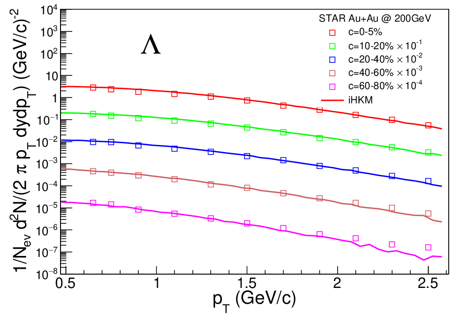
In Figs. 12, 13 the results for , and hyperon spectra are demonstrated, as well as the comparison of values, used in the model, and those extracted within the experimental analysis from the Boltzmann fits to the measured spectra star_bar. The model curves for hyperon spectra agree with the data and the utilized factors coincide with the experimental ones within the error bars.


III.4 Femtoscopy scales
The correlation femtoscopy is a powerful experimental technique, that allows to reveal the space-time structure of the system, formed in relativistic heavy-ion collision, presenting it in terms of the interferometry (femtoscopy) radii. The latter are extracted from the Gaussian fits to the experimentally measured two-particle momentum correlation functions of identical particles in each bin. Each is commonly interpreted as the homogeneity length of the system in direction, related to the region, where the particles with momenta close to are mostly emitted from Sin1; Sin2; AkkSin2.
The iHKM provides a satisfactory description of the femtoscopy radii in the considered high-energy collision experiments, for which the experimental data are available for comparison (except, maybe, for a somewhat overestimated pion radii in the top RHIC energy Au+Au collisions at rhic-ihkm, as compared to the PHENIX Collaboration results), and allows to obtain predictions for not yet measured data (see Fig. 8).
The observed in iHKM behaviour of the radii with is quite similar at all the collision energies. At the fixed centrality the radii values grow by , when going from the RHIC to the LHC, and the radii, related to the different LHC energies are very close, with differences not exceeding . Such similarity of the femtoscopy scales for the LHC collisions, that takes place despite the differences in the system geometric sizes at the freeze-out stage, can be explained by the fact, that collective flow velocity gradients are higher at larger energies, and so this compensates the different geometry influence, resulting in close lengths of homogeneity in the considered cases Sin1; AkkSin2.
An approximate scaling, that can be observed in Fig. 8 between kaon and pion femtoscopy radii at GeV/, was firstly noticed for the LHC Pb+Pb collisions at TeV in iHKM simulations ourkt and then confirmed in the experimental analysis alice-scaling.
In the current paper we also present the comparison of the interferometry scales, obtained in iHKM simulations for the high-energy collision events with close charged particle multiplicities. Such a comparison has an aim to check the so-called “scaling hypothesis” (see, e.g. Lisa1; Lisa2), supposing that the interferometry radii and the corresponding interferometry volume grow almost linearly with the mean charged particle density . Despite the fact the scaling hypothesis is often assumed in femtoscopy studies, we believe, that the femtoscopy scales should depend also on geometrical sizes of the colliding ions (see Fig. 14), as it was previously noticed in scaling1; scaling2; pp-lhc.
| Experiment | Centrality (%) | |
|---|---|---|
| Au+Au @ 200 GeV | 688 | |
| Pb+Pb @ 2.76 TeV | 693 | |
| Pb+Pb @ 5.02 TeV | 677 | |
| Xe+Xe @ 5.44 TeV | 680 |


To investigate this issue, for all the considered collision types we selected the events of different centralities, such that the mean charged particle multiplicities in each case were nearly equal (see Table 2). Then we built the graphs of pion and kaon interferometry volume dependencies on parameter, which characterizes the sizes of the initial transverse overlapping of the two colliding nuclei (see Fig. 15). This parameter is calculated as the area of nearly elliptical cross-section of the initial energy-density profile at the half-value of the maximal initial energy density ,
| (22) |
where and are the semi-axes of the ellipse. The values were also divided by the corresponding mean charged particle multiplicities to avoid the effect of still existing small differences in between the experimental set-ups.
From Fig. 15 it follows that the plotted reduced volume grows with , having the smallest value for the LHC Pb+Pb collisions at TeV, a somewhat higher value in the TeV case, after which follows the volume in Xe+Xe collisions at TeV, and the highest one is the value for Au+Au collisions at GeV. The next plot in Fig. 16 shows the individual kaon interferometry radii dependencies on the pair for the analyzed collision experiments together with the corresponding re-scaled initial energy density profiles . One can see, that the differences between the values, observed in Fig. 15, are mainly due to the differences in the corresponding transverse radii. The contribution from radius is the principal one, the contribution is smaller, and the radii in all the considered cases practically coincide. The obtained results confirm the assumption, made in scaling1; scaling2; pp-lhc, that the origin of the observed differences between the interferometry volumes is in different transverse flow velocities, which develop in the analyzed systems because of the different initial geometric sizes and the energy/pressure gradients.

Based on the combined fitting of the longitudinal femtoscopy radii dependency on and the transverse momentum spectrum, one can estimate the time of maximal emission for particles of a given species mtscale, i.e. the effective time, that can be associated with the maximal intensity of the emission process, when the corresponding particles most actively leave the system. The presented method was applied by the ALICE Collaboration for the extraction of pion and kaon times of maximal emission from the experimental data alice-scaling.
The first step is to perform a combined fitting of pion and kaon spectra with the formula
| (23) |
where is the effective temperature, is the parameter, describing the strength of collective flow in such a way, that the infinite means zero flow, and small means strong flow, is the transverse collective velocity at the saddle point, (see Ref. mtscale for details). From the fit one extracts the common effective temperature of pions and kaons and the two values for each particle sort.
At the second step one should carry out the fitting of dependencies for pions and kaons using the formula
| (24) |
where is expressed through the longitudinal homogeneity length of the system , , and is the maximal emission time, the one is interested in. When performing this fit, the and parameters should be constrained within the limits, defined earlier during the spectra fitting. However, the parameter for kaons should be left unconstrained. As a result, one extracts from the fit the desired times of maximal emission and . In the paper rhic-ihkm we obtained the values fm/ and fm/. These results support the hypothesis about the continuous character of particle emission and freeze-out in high-energy heavy-ion collisions.
III.5 Direct photon production
In spite of the hadrons, that are formed at the last stage of superdense system evolution, the direct photon production is accumulated from the different sources along with the process of relativistic heavy ion collision developing. Those include the primary hard photons from the parton collisions at the very early stage of the process, the photons generated at the pre-thermal phase of dense matter evolution, then thermal photons at partially equilibrated hydrodynamic quark-gluon stage, and, finally, from the hadron gas phase. All the phases of evolution are presented in iHKM, therefore, the corresponding calculations with initial conditions providing a good description all the bulk hadron observables (see previous discussions) were done in the model for top RHIC photons2 and LHC photons1 energies.
Along the way a hadronic medium evolution is treated in two distinct, in a sense opposite, approaches: chemically equilibrium and chemically non-equilibrium, namely, chemically frozen expansion. We find the description of direct photon spectra, elliptic and triangular flow are significantly improved, for both RHIC the LHC energies, if an additional portion of photon radiation associated with the confinement processes, the “hadronization photons”, is included into consideration. In iHKM this contribution is introduced with only one free parameter, characterizing intensity of the photon radiation at the confinement process. This parameter is fixed from fitting the direct photon spectra in most central events, and used then at all centralities for spectra, as well as for description of elliptic and triangular photon flow. Figure 17 demonstrates the iHKM results for RHIC and LHC photon spectra in central events () with and without this hadronization emission (HE). The iHKM results for RHIC (centrality 20-40%) photon elliptic and triangular flows are demonstrated in Fig. 18.


The problem of serious underestimation of direct photon production, as well as their flows in theoretical models as compared to the experimental data is called “direct photon puzzle”. From our results it can be concluded, that photon radiation in the pseudo-critical region is, probably, a key to solve the photon puzzle.
IV Conclusions
The integrated hydrokinetic model, which simulates the full process of the matter evolution in course of the relativistic heavy-ion collision, including early pre-equilibrium relaxation dynamics, that transforms the initially non-equilibrated state of the system to a nearly thermalized one, allows one to obtain a comprehensive description of measured bulk observables and to reveal underlying dynamics of the collision process and its femtoscopic space-time structure. The early start of the system’s evolution in iHKM (at proper time about fm/) allows to account for pre-thermal development of the collective effects and thus improve the data description.
The model provides a simultaneous description of particle yields and their ratios, hadron and photon spectra and flow harmonics. Also a good description and succesfull prediction of pion and kaon femtoscopy radii for all the modern ultrarelativistic heavy-ion collision experiments (Au+Au collisions at the RHIC energy GeV, Pb+Pb collisions at the LHC energies TeV and TeV, Xe+Xe collisions at the LHC energy TeV) using a single parameter set in each case. To re-calibrate iHKM, switching from the simulation of one of the mentioned collision types to another, one basically needs to change only two parameters, and , and to go from the LHC energy TeV to TeV — only one parameter, .
The simulations carried out using the two different equations of state for quark-gluon phase with the corresponding particlization temperatures demonstrate, that an equally good description of data can be achieved in both cases, provided the initial maximal energy density parameter is retuned. This result together with the results of probing the hadronic medium with resonance, showing that intensive interactions between hadrons take place at least during 5 fm/ after particlization, speak in favor of continuous character of chemical and kinetic freeze-outs and indicate a great role of the afterburner stage of heavy ion collision in the formation of measured observables.
The iHKM results for the interferometry volumes and radii, obtained for different colliding nuclei in events with close charged particle multiplicities, allow to conclude, that the hypothesis about scaling of the femtoscopy radii with multiplicity is not confirmed. The transverse interferometry radii, and hence, the interferometry volume, depend also on geometric sizes of the colliding nuclei and grow with the transverse area of their overlapping right after collision.
The investigation of the “direct photon puzzle” within iHKM demonstrates that account for the photon radiation during the confinement process in the pseudo-critical region can help to solve the problem and provide a good description of the direct photon spectra and flow harmonics.
Acknowledgements.
The research was carried out within the project “Spatiotemporal dynamics and properties of superdense matter in relativistic collisions of nuclei, and their signatures in current experiments at the LHC, RHIC and planned FAIR, NICA”. Agreement № 7/2020 with NAS of Ukraine. It is partially supported by COST Action THOR (CA15213).References
- (1) B. Mueller, A. Schaefer, Int. J. Mod. Phys. E 20, 2235 (2011).
- (2) J. Berges, K. Boguslavski, S. Schlichting, R. Venugopalan, Phys. Rev. D 89, 114007 (2014).
- (3) J.-P. Blaizot, B. Wu, L. Yan, Nucl. Phys. A 930, 139 (2014).
- (4) O. DeWolfe, S.S. Gubser, C. Rosen, D. Teaney, Progr. Part. Nucl. Phys. 75, 86 (2014).
- (5) S.V. Akkelin, Yu.M. Sinyukov, Phys. Rev. C 89, 034910 (2014).
- (6) X.-G. Huang, J. Liao, Int. J. Mod. Phys. E 23, 1430003 (2014).
- (7) R. Venugopalan, Nucl. Phys. A 928, 209 (2014).
- (8) A. Kurkela, E. Lu, Phys. Rev. Lett. 113, 182301 (2014).
- (9) J. Berges, B. Schenke, S. Schlichting, R. Venugopalan, Nucl. Phys. A 931, 348 (2014).
- (10) S. A. Bass et al., Prog. Part. Nucl. Phys. 41 (1998) 255.
- (11) M. Bleicher et al., J. Phys. G 25 (1999) 1859.
- (12) Y. Nara, N. Otuka, A. Ohnishi, K. Niita and S. Chiba, Phys. Rev. C 61, 024901 (2000).
- (13) C. Nonaka and S. A. Bass, Phys. Rev. C 75, 014902 (2007).
- (14) T. Hirano, U. W. Heinz, D. Kharzeev, R. Lacey and Y. Nara, Phys. Rev. C 77, 044909 (2008).
- (15) S. Pratt and J. Vredevoogd, Phys. Rev. C 78, 054906 (2008) [Erratum-ibid. C 79, 069901 (2009)].
- (16) H. Petersen, Phys. Rev. C 84, 034912 (2011).
- (17) K. Werner, I. Karpenko and T. Pierog, Phys. Rev. Lett. 106, 122004 (2011).
- (18) H. Song, S. A. Bass and U. Heinz, Phys. Rev. C 83, 054912 (2011).
- (19) V.Yu. Naboka, S.V. Akkelin, Iu.A. Karpenko, Yu.M. Sinyukov, Phys. Rev. C 91, 014906 (2015).
- (20) V.Yu. Naboka, Iu.A. Karpenko, Yu.M. Sinyukov, Phys. Rev. C 93, 024902 (2016);
- (21) W. Broniowski, M. Rybczynski, P. Bozek, Comput. Phys. Commun. 180 (2009) 69.
- (22) H. J. Drescher and Y. Nara, Phys. Rev. C 75 034905 (2007).
- (23) F. Gelis, E. Iancu, J. Jalilian-Marian, R. Venugopalan, Ann. Rev. Nucl. Part. Sci. 60, 463 (2010)
- (24) Yu.M. Sinyukov, S.V. Akkelin, Y. Hama, Phys. Rev. Lett. 89, 052301 (2002).
- (25) S.V. Akkelin, Y. Hama, Iu.A. Karpenko, Yu.M. Sinyukov, Phys. Rev. C 78, 034906 (2008).
- (26) Yu.M. Sinyukov, S.V. Akkelin, Iu.A. Karpenko, Y. Hama, Acta Phys. Polon. B 40, 1025 (2009).
- (27) Yu.A. Karpenko, Yu.M. Sinyukov, J. Phys. G: Nucl. Part. Phys. 38, 124059 (2011).
- (28) Iu.A. Karpenko, Yu.M. Sinyukov, K. Werner, Phys. Rev. C 87, 024914 (2013).
- (29) Yu.M. Sinyukov, S.V. Akkelin, Iu.A. Karpenko, V.M. Shapoval, Advances in High Energy Physics, Vol. 2013, Article ID 198928.
- (30) Yu. M. Sinyukov, V. M. Shapoval, Phys. Rev. C 97, 064901 (2018).
- (31) V. M. Shapoval, Yu. M. Sinyukov, Phys. Rev. C 100, 044905 (2019).
- (32) M. D. Adzhymambetov, V. M. Shapoval, and Yu. M. Sinyukov, Nucl. Phys. A, 987 (2019) 321.
- (33) V.M. Shapoval, P. Braun-Munzinger, Yu.M. Sinyukov, Nucl. Phys. A 968, 391 (2017).
- (34) V. Yu. Naboka, Yu. M. Sinyukov, G. M. Zinovjev, Phys. Rev. C 97, 054907 (2018).
- (35) V. Yu. Naboka, Yu. M. Sinyukov, G. M. Zinovjev, Nucl. Phys. A, 1000 (2020) 121843.
- (36) S. Acharya et al. (ALICE Collaboration), Phys. Lett. B 788 (2019) 166-179.
- (37) S. Ragoni (for the ALICE Collaboration), arXiv:1809.01086 [hep-ex].
- (38) L. Tinti, W. Florkowski, Phys. Rev. C 89, 034907 (2014).
- (39) D. Bazow, U. Heinz, M. Strickland, Phys. Rev. C 90, 054910 (2014).
- (40) U. Heinz, D. Bazow, M. Strickland, Nucl. Phys. A 931, 920 (2014).
- (41) S. V. Akkelin and Yu. M. Sinyukov, Phys. Rev. C 81 (2010) 064901.
- (42) J. D. Bjorken, Phys. Rev. D 27, 140 (1983).
- (43) Iu. Karpenko, P. Huovinen, M. Bleicher, Comput. Phys. Commun. 185, 3016 (2014).
- (44) M. Laine and Y. Schroeder, Phys. Rev. D 73, 085009 (2006).
- (45) A. Bazarov et al. (The HotQCD Collaboration), Phys. Rev. D 90, 094503 (2014).
- (46) J. Stachel, A. Andronic, P. Braun-Munzinger and K. Redlich, J. Phys. Conf. Ser. 509, 012019 (2014).
- (47) F. Karsch, arXiv:0711.0656.
- (48) P. Huovinen, H. Petersen, Eur. Phys. J. A 48, 171 (2012).
- (49) S. Pratt, Phys. Rev. C 89, 024910 (2014).
- (50) D. Molnar, Z. Wolff, Phys. Rev. C 95, 024903 (2017).
- (51) D. Molnar, J. Phys. G 38, 124173 (2011).
- (52) T. Lappi, Phys. Lett. B643, 11 (2006).
- (53) B. Abelev et al. (The ALICE Collaboration), Phys. Rev. Lett. 109 (2012) 252301.
- (54) B. Abelev et al. (The ALICE Collaboration), Phys. Rev. C 88 (2013) 044910.
- (55) F. Becattini et al. in New Horizons in Fundamental Physics (Springer, 2016), pp. 139-150.
- (56) S. Chatterjee, R.M. Godbole, S. Gupta, Phys. Lett. B 727 (2013) 554.
- (57) F. Bellini (for the ALICE Collaboration), Nucl. Phys. A 982, 427 (2019).
- (58) D.S.D. Albuquerque (for the ALICE Collaboration), Nucl. Phys. A 982, 823 (2019).
- (59) N. Jacazio (for the ALICE Collaboration), Nucl. Phys. A 967, 421 (2017).
- (60) J. Adams et al. (The STAR Collaboration), Phys. Rev. C 72 (2005) 014904.
- (61) J. Adam et al. (The ALICE Collaboration), Phys. Rev. Lett. 116, 132302 (2016).
- (62) M. Floris, Nucl. Phys. A 931 (2014) 103-112.
- (63) J. Adams et al. (The STAR Collaboration), Phys. Rev. Lett. 98, 062301 (2007).
- (64) Yu. M. Sinyukov, Nucl. Phys. A 566, 589 (1994).
- (65) Yu.M. Sinyukov, in Hot Hadronic Matter: Theory and Experiment, edited by J. Letessier, H. H. Gutbrod and J. Rafelski (Plenum, New York, 1995), p. 309.
- (66) S.V. Akkelin, Yu.M. Sinyukov, Phys. Lett. B 356, 525 (1995).
- (67) V. M. Shapoval, P. Braun-Munzinger, Iu. A. Karpenko, Yu. M. Sinyukov, Nucl. Phys. A 929 (2014) 1.
- (68) J. Adam et al. (The ALICE Collaboration), Phys. Rev. C 96, 064613 (2017).
- (69) M. Lisa, S. Pratt, R. Soltz, U. Wiedemann. Ann. Rev. Nucl. Part. Sci. 55 (2005) 357.
- (70) M. Lisa, Braz. J. Phys. 37 (2007) 963.
- (71) S.V. Akkelin, Yu.M. Sinyukov, Phys. Rev. C 70 (2004) 064901.
- (72) S.V. Akkelin, Yu.M. Sinyukov, Phys. Rev. C 73 (2006) 034908.
- (73) V. M. Shapoval, P. Braun-Munzinger, Iu. A. Karpenko, and Yu. M. Sinyukov, Phys. Lett. B 725 (2013) 139.
- (74) K. Aamodt, et al. (The ALICE Collaboration), Phys. Rev. D 84 (2011) 112004.
- (75) K. Aamodt, et al. (The ALICE Collaboration), Phys. Lett. B 696 (2011) 328.
- (76) D. Antonczyk, Acta Phys. Polon. B 40 (2009) 1137.
- (77) S.V. Afanasiev et al. (The NA49 Collaboration), Phys. Rev. C 66 (2002) 054902.
- (78) C. Alt et al. (The NA49 Collaboration), Phys. Rev. C 77 (2008) 064908.
- (79) J. Adams et al. (The STAR Collaboration), Phys. Rev. Lett. 92 (2004) 112301.
- (80) J. Adams et al. (The STAR Collaboration), Phys. Rev. C 71 (2004), 044906.
- (81) S. S. Adler et al. (The PHENIX Collaboration), Phys. Rev. C 69 (2004) 034909.
- (82) S. S. Adler et al. (The PHENIX Collaboration), Phys. Rev. Lett. 93 (2004) 152302.
- (83) Yu.M. Sinyukov, V.M. Shapoval, V.Yu. Naboka, Nucl. Phys. A 946, 227 (2016).
- (84) A. Adare et al. (The PHENIX Collaboration), Phys. Rev. C 91 (2015) 064904.
- (85) A. Adare et al. (The PHENIX Collaboration), Phys. Rev. C 94 (2016) 064901.
- (86) J. Adam et al. (The ALICE Collaboration), Phys. Lett. B 754, 235 (2016).