Constructive Universal High-Dimensional Distribution Generation through Deep ReLU Networks

Dmytro Perekrestenko Affiliation: Department of Information Technology and Electrical Engineering, ETH Zürich, Zürich, Switzerland Correspondence to: pdmytro@mins.ee.ethz.ch Stephan Müller Affiliation: Department of Information Technology and Electrical Engineering, ETH Zürich, Zürich, Switzerland Helmut Bölcskei Affiliation: Department of Information Technology and Electrical Engineering, ETH Zürich, Zürich, Switzerland Affiliation: Department of Mathematics, ETH Zürich, Zürich, Switzerland

Abstract

We present an explicit deep neural network construction that transforms uniformly distributed one-dimensional noise into an arbitrarily close approximation of any two-dimensional Lipschitz-continuous target distribution. The key ingredient of our design is a generalization of the “space-filling” property of sawtooth functions discovered in (Bailey & Telgarsky 2018). We elicit the importance of depth—in our neural network construction—in driving the Wasserstein distance between the target distribution and the approximation realized by the network to zero. An extension to output distributions of arbitrary dimension is outlined. Finally, we show that the proposed construction does not incur a cost—in terms of error measured in Wasserstein-distance—relative to generating $d$ -dimensional target distributions from $d$ independent random variables.

Keywords:

Machine Learning, Approximation Theory, Generative Networks, ICML

1 Introduction

Deep neural networks have been used very successfully as generative models for complex natural data such as images (Radford et al. 2016; Karras et al. 2019) and natural language (Bowman et al. 2016; Xu et al. 2018). Specifically, the idea is to learn the parameters of deep networks (Kingma & Welling 2014; Goodfellow et al. 2014) so that they realize complex high-dimensional probability distributions by transforming samples taken from simple low-dimensional distributions such as uniform or Gaussian.

Generative networks with higher output than input dimension occur, for instance, in language modelling where deep networks are used to predict the next word in a text sequence. Here, the input layer size is determined by the dimension of the word embedding (typically $\sim 100$ ) and the output layer, representing a vector of probabilities for each of the words in the vocabulary, is of the size of the vocabulary (typically $\sim 100k$ ). Another example where the dimensionality of the input distribution is mandated to be lower than that of the output distribution is given by the variational inference methods according to (Kingma & Welling 2014; Tolstikhin et al. 2018).

Notwithstanding the practical success of deep generative networks, a profound theoretical understanding of their representational capabilities is still lacking. First results along those lines appear in (Lee et al. 2017), which establishes that generative networks can approximate distributions arising from the composition of Barron functions (Barron 1993).

Bailey and Telgarsky (Bailey & Telgarsky 2018) show how deep ReLU networks can be used to increase the dimensionality of uniform distributions and how a univariate uniform distribution can be turned into a univariate Gaussian distribution and vice versa. Finally, (Lu & Lu 2020) shows that neural networks constitute universal approximators for continuous probability distributions when source and target distribution are of the same dimension.

Classical approaches for generating multi-dimensional random variables of a given distribution such as the Box-Muller method (Box & Muller 1958) or conditional distribution, rejection, and composition methods (Devroye 1986) are all based on transforming initial distributions of the same dimensionality as the target distribution. We are not aware of methods that map one-dimensional inputs to prescribed $d$ -dimensional outputs. The purpose of the present paper is to show that deep generative networks are capable of doing exactly that and moreover are also universal generators, in contrast to, e.g., the Box-Muller method (Box & Muller 1958), which maps uniform distributions to Gaussian distributions, albeit with zero error. We also quantify how the connectivity of the resulting networks scales with the approximation error measured in Wasserstein distance.

The problem is approached in two steps. Specifically, given a two-dimensional Lipschitz-continuous target distribution, we first find the (two-dimensional) histogram distribution that best approximates it—for a given histogram resolution—in Wasserstein distance. The resulting histogram distribution is then realized by a ReLU network driven by a uniform univariate input distribution. To this end, we develop a new space-filling property of ReLU networks, generalizing that discovered in (Bailey & Telgarsky 2018). The main conceptual insight of this paper is that generating arbitrary $d$ -dimensional target distributions, with $d\geq 2$ , from a one-dimensional uniform distribution through a deep neural network does not come at a cost—in terms of approximation error measured in Wasserstein distance—relative to generating the target distribution from $d$ independent random variables. We emphasize that the generating network has to be deep, in fact the depth has to go to infinity to obtain the same error in Wasserstein-distance as a construction from $d$ independent random variables would yield.

We finally note that our results pertain only to representational capabilities of generative (ReLU-)networks and we do not consider the problem of learning the network weights and biases.

1.1 Notation and Definitions

We denote the set of integers in the range $[1,n]$ by $[[1,n]]$ . $U(\Delta)$ stands for the uniform distribution on the interval $\Delta$ , when $\Delta=[0,1]$ , we simply write $U$ . Given a probability distribution with pdf $p$ , we denote the push-forward of $p$ under the function $f$ as $f\#p$ . For a given compact set ${\cal C}$ , we let $p_{\mathbf{X}}(\mathbf{x}\in{\cal C})=\int_{\cal C}p_{\mathbf{X}}(\mathbf{x})d\mathbf{x}$ . We define ReLU neural networks as follows.

Definition 1.1.

Let $L,N_{0},N_{1},\ldots,N_{L}\in\mathbb{N}$ , $L\geq 2$ . A map $\Phi:\mathbb{R}^{N_{0}}\to\mathbb{R}^{N_{L}}$ given by

\Phi(x)=\begin{cases}\begin{array}[]{lc}\hskip-2.84544ptW_{2}(\rho\,(W_{1}(x))),&L=2\\ \hskip-2.84544ptW_{L}(\rho\,(W_{L-1}(\rho\,(\dots\rho\,(W_{1}(x)))))),&L\geq 3\end{array},\end{cases}

with affine linear maps $W_{\ell}:\mathbb{R}^{N_{\ell-1}}\to\mathbb{R}^{N_{\ell}}$ , $\ell\in\{1,2,\dots,L\}$ , and the ReLU activation function $\rho(x)=\max(x,0),\ x\in\mathbb{R}$ , acting component-wise (i.e., $\rho(x_{1},\dots,x_{N}):=(\rho(x_{1}),\dots,\rho(x_{N}))$ ) is called a ReLU neural network. The map $W_{\ell}$ corresponding to layer $\ell$ is given by $W_{\ell}(x)=A_{\ell}x+b_{\ell}$ , with $A_{\ell}\in\mathbb{R}^{N_{\ell}\times N_{\ell-1}}$ and $b_{\ell}\in\mathbb{R}^{N_{\ell}}$ . We define the network connectivity $\mathcal{M}(\Phi)$ as the total number of non-zero entries in the matrices $A_{\ell}$ , $\ell\in\{1,2,\dots,L\}$ , and the vectors $b_{\ell}$ , $\ell\in\{1,2,\dots,L\}$ . The depth of the network or, equivalently, the number of layers is $\mathcal{L}(\Phi):=L$ and its width is given by $\mathcal{W}(\Phi):=\max_{\ell=0,\dots,L}N_{\ell}$ . We denote by $\mathcal{N}_{d,d^{\prime}}$ the set of ReLU networks with input dimension $N_{0}=d$ and output dimension $N_{L}=d^{\prime}$ .

We measure the distance between distributions in terms of Wasserstein distance defined as follows.

Definition 1.2.

Let $\mu$ and $\nu$ be distributions on $\mathbb{R}^{d}$ and denote the set of distributions on $\mathbb{R}^{d}\times\mathbb{R}^{d}$ whose first and second marginals coincide with $\mu$ and $\nu$ , respectively, by $\prod(\mu,\nu)$ . Then, the Wasserstein distance between $\mu$ and $\nu$ is defined as

W(\mu,\nu):=\inf_{\pi\in\prod(\mu,\nu)}\int|x-y|d\pi(x,y),

where the elements of the set $\prod(\mu,\nu)$ are called couplings of $\mu$ and $\nu$ .

Definition 1.3.

For distributions $\mu$ and $\nu$ on $\mathbb{R}^{d}$ with corresponding pdfs $p_{\mu},p_{\nu}$ supported on $\Omega\subset\mathbb{R}^{d}$ , the total variation (TV) distance is defined as

TV(\mu,\nu):=\frac{1}{2}||p_{\mu}-p_{\nu}||_{L_{1}(\Omega)}.

The following relation between Wasserstein distance and TV-distance was found in (Gibbs & Su 2002).

Theorem 1.4.

(Gibbs & Su 2002) For distributions $\mu$ and $\nu$ on $\mathbb{R}^{d}$ with pdfs $p_{\mu},p_{\nu}$ supported on $\Omega\subset\mathbb{R}^{d}$ , the Wasserstein distance and the TV-distance satisfy

W(\mu,\nu)\leq\text{diam}(\Omega)\cdot TV(\mu,\nu),

where $\text{diam}(\Omega)=\sup\{|x-y|:x,y\in\Omega\}$ .

Next, we define $d$ -dimensional histogram distributions.

Definition 1.5.

A random vector $\mathbf{X}=(X_{1},X_{2},\dots,X_{d})$ is said to have a general histogram distribution of resolution $n$ on the $d$ -dimensional unit cube, denoted as $\mathbf{X}\sim\mathcal{G}[0,1]^{d}_{n}$ , if for some $0=t^{j}_{0}<t^{j}_{1}<\dots<t^{j}_{n}=1$ , $j\in[[1,d]]$ , its pdf is given by

	$\displaystyle p(\mathbf{x})$	$\displaystyle=\sum_{\mathbf{k}}w_{\mathbf{k}}\chi_{c_{\mathbf{k}}}(\mathbf{x}),\quad\sum_{\mathbf{k}}w_{\mathbf{k}}\prod_{j=1}^{d}(t^{j}_{i_{j}+1}-t^{j}_{i_{j}})=1,$
		$\displaystyle w_{\mathbf{k}}>0,\ \ \text{for all}\ \ \mathbf{k}\in[[0,n-1]]^{d},$

where $\mathbf{k}=(i_{1},i_{2},\dots,i_{d})\in[[0,n-1]]^{d}$ is an index vector and $\chi_{c_{\mathbf{k}}}(\mathbf{x})$ is the characteristic function of the $d$ -dimensional cube $c_{\mathbf{k}}=[t^{1}_{i_{1}},t^{1}_{i_{1}+1}]\times[t^{2}_{i_{2}},t^{2}_{i_{2}+1}]\times\dots\times[t^{d}_{i_{d}},t^{d}_{i_{d}+1}]$ .

We will mostly be concerned with histogram distributions of uniform tile size, defined as follows.

Definition 1.6.

A random vector $\mathbf{X}=(X_{1},X_{2},\dots,X_{d})$ is said to have a histogram distribution of resolution $n$ on the $d$ -dimensional unit cube, denoted as $\mathbf{X}\sim\mathcal{E}[0,1]_{n}^{d}$ , if its pdf is given by

	$\displaystyle p(\mathbf{x})$	$\displaystyle=\sum_{\mathbf{k}}w_{\mathbf{k}}\chi_{c_{\mathbf{k}}}(\mathbf{x}),\quad\sum_{\mathbf{k}}w_{\mathbf{k}}=n^{d},$
		$\displaystyle w_{\mathbf{k}}>0,\ \ \text{for all}\ \ \mathbf{k}\in[[0,n-1]]^{d},$

where $\mathbf{k}=(i_{1},i_{2},\dots,i_{d})\in[[0,n-1]]^{d}$ is an index vector and $\chi_{c_{\mathbf{k}}}(\mathbf{x})$ is the characteristic function of the $d$ -dimensional cube $c_{\mathbf{k}}=[i_{1}/n,(i_{1}+1)/n]\times[i_{2}/n,(i_{2}+1)/n]\times\dots\times[i_{d}/n,(i_{d}+1)/n]$ .

Remark 1.7.

For ease of exposition, in Definitions 1.5 and 1.6, we let $c_{\mathbf{k}}$ be a product of closed intervals, thus allowing the breakpoints to belong to different cubes. While this comes without loss of generality, for concreteness, it is understood that the value of the pdf at the breakpoints is the average across the cubes the corresponding breakpoint belongs to.

2 Universal approximation

As mentioned in the introduction, the intermediate step in our construction consists of a ReLU network that turns a univariate one-dimensional input distribution into a two-dimensional histogram distribution. This histogram distribution is then chosen such that it approximates the two-dimensional Lipschitz-continuous target distribution. To understand why we chose this two-step approach, note that ReLU networks generate piecewise linear functions and the pushforward $f\#U$ of any piecewise linear $f:\mathbb{R}\rightarrow\mathbb{R}$ yields a histogram distribution. We start by quantifying the TV distance between an arbitrary distribution and a histogram distribution of resolution $n$ .

Theorem 2.1.

Let $p$ be a $d$ -dimensional L-Lipschitz-continuous pdf of finite differential entropy on its support $[0,1]^{d}$ . Then, for every $n>0$ , there exists a $\tilde{p}\in\mathcal{E}[0,1]_{n}^{d}$ such that

TV(p,\tilde{p})=\frac{1}{2}\|p-\tilde{p}\|_{L_{1}([0,1]^{d})}\leq\frac{L\sqrt{d}}{2n}.

Proof.

The proof is based on the Mean Value Theorem, which states that, for any continuous $d$ -dimensional function $p$ supported on $\Omega\in\mathbb{R}^{d}$ , there exists a $\mathbf{z}\in\Omega$ , such that

\int_{\Omega}p(\mathbf{x})d\mathbf{x}=p(\mathbf{z})\int_{\Omega}d\mathbf{x}.

(1)

Next, we divide the unit cube $[0,1]^{d}$ into the $n^{d}$ cubes $c_{\mathbf{k}}$ per Definition 1.6. Take an arbitrary $\mathbf{k}\in[[0,n-1]]^{d}$ and fix $\mathbf{z}_{\mathbf{k}}$ according to Equation 1 with $\Omega=c_{\mathbf{k}}$ . Then, using the Lipschitz property of $p$ , we obtain

		$\displaystyle\\|p(\mathbf{x})-p(\mathbf{z}_{\mathbf{k}})\\|_{L_{1}(c_{\mathbf{k}})}=\int_{c_{\mathbf{k}}}\|p(\mathbf{x})-p(\mathbf{z}_{\mathbf{k}})\|d\mathbf{x}$
		$\displaystyle\leq\int_{c_{\mathbf{k}}}L\|\mathbf{x}-\mathbf{z}_{\mathbf{k}}\|d\mathbf{x}\leq\int_{c_{\mathbf{k}}}L\frac{\sqrt{d}}{n}d\mathbf{x}=L\frac{\sqrt{d}}{n}\cdot\frac{1}{n^{d}}.$

We set

\tilde{p}(\mathbf{x})=\sum_{\mathbf{k}}p(\mathbf{z}_{\mathbf{k}})\chi_{c_{\mathbf{k}}}(\mathbf{x})

and note that $\tilde{p}\in\mathcal{E}[0,1]_{n}^{d}$ as $\sum_{\mathbf{k}}p(\mathbf{z}_{\mathbf{k}})=n^{d}$ owing to Equation 1; moreover, $p(\mathbf{z}_{\mathbf{k}})>0$ , for all $\mathbf{k}$ , as $p$ is of finite differential entropy on $[0,1]^{d}$ . Finally, summing up across all cubes $c_{\mathbf{k}}$ , we obtain

	$\displaystyle\\|p-\tilde{p}\\|_{L_{1}{([0,1]^{d})}}$	$\displaystyle=\int_{[0,1]^{d}}\|p(\mathbf{x})-\tilde{p}(\mathbf{x})\|d\mathbf{x}$
		$\displaystyle\leq\sum_{\mathbf{k}}\int_{c_{\mathbf{k}}}L\|\mathbf{x}-\mathbf{z}_{\mathbf{k}}\|d\mathbf{x}\leq L\frac{\sqrt{d}}{n}.\hskip 8.5359pt\qed$

Henceforth, we shall always assume that probability density functions $p$ are of finite differential entropy on their support, without explicitly declaring it.

We are now ready to state the main result of the paper, the proof of which is largely based on Theorem 4.4 below.

Theorem 2.2.

Let $p_{X,Y}$ be an $L$ -Lipschitz-continuous pdf supported on $[0,1]^{2}$ . Then, for every $n>0$ , there exists a $\Phi\in\mathcal{N}_{1,2}$ with connectivity $\mathcal{M}(\Phi)\leq 88(n^{2}+ns)$ and of depth $\mathcal{L}(\Phi)=s+5$ , such that

W(\Phi\#U,p_{X,Y})\leq\frac{L\sqrt{2}}{2n}+\frac{2\sqrt{2}}{n2^{s}}.

Proof.

Combining Theorem 2.1 with Theorem 1.4, we obtain that for every $n>0$ , there exists a $\tilde{p}\in\mathcal{E}[0,1]_{n}^{2}$ such that

W(p,\tilde{p})\leq\frac{L}{n}.

On the other hand, it follows from Theorem 4.4 that, for every $\tilde{p}\in\mathcal{E}[0,1]_{n}^{2}$ , there exists a neural network $\Phi\in\mathcal{N}_{1,2}$ with connectivity $\mathcal{M}(\Phi)\leq 88(n^{2}+ns)$ and of depth $\mathcal{L}(\Phi)=s+5$ such that

W(\Phi\#U,\tilde{p})\leq\frac{2\sqrt{2}}{n2^{s}}.

We finalize the proof by application of the triangle inequality for Wasserstein distance (Clement & Desch 2008) to get

	$\displaystyle W(\Phi\#U,p)$	$\displaystyle\leq W(\Phi\#U,\tilde{p})$
		$\displaystyle+W(p,\tilde{p})=\frac{L}{n}+\frac{2\sqrt{2}}{n2^{s}}.\hskip 34.14322pt\qed$

The error bound in Theorem 2.2 illustrates the main conceptual insight of this paper, namely that generating arbitrary two-dimensional Lipschitz-continuous distributions from a one-dimensional uniform distribution through a deep neural network does not come at a cost—in terms of Wasserstein-distance error—relative to generating this two-dimensional target distribution from two independent random variables. Specifically, if we let the depth $s$ of the generating network go to infinity, the second term in the error bound will go to zero exponentially fast in $s$ leaving us only with the first term, which reflects the error stemming from the histogram approximation of the distribution. Moreover, this first term is inversely proportional to the histogram resolution $n$ and linear in the Lipschitz constant and can thus be made arbitrarily small by letting the histogram resolution $n$ approach infinity. The width of the corresponding generating network will grow according to $n^{2}$ . When the target distribution is uniform, we recover the result in (Bailey & Telgarsky 2018). The intermediate step via histogram distributions was not needed in (Bailey & Telgarsky 2018) as Bailey and Telgarsky only considered mapping uniform input distributions to uniform output distributions. Finally, we note that our result carries over to general $d$ -dimensional output distributions; we briefly comment on this extension in Section 5.

3 ReLU networks and histograms

This section systematically establishes the connection between ReLU networks and histogram distributions. Specifically, we show that the pushforward of a uniform distribution under a piecewise linear function results in a histogram distribution. We will also identify, for a given histogram distribution, the corresponding piecewise linear function generating it under pushforward of a uniform distribution. Combined with the insight that ReLU networks always realize piecewise linear functions, we will have established the desired connection.

We start with a simple auxiliary result.

Lemma 3.1.

Let $a,b\in\mathbb{R},a<b,\Delta=[a,b]$ , and let $h(x)=mx+s$ , for $x\in\mathbb{R}$ , with $m\in\mathbb{R}\setminus\{0\},s\in\mathbb{R}$ . Then, $Q=h\#U(\Delta)$ is uniformly distributed on $[ma+s,mb+s]$ , for $m>0$ , and on $[mb+s,ma+s]$ , for $m<0$ .

Proof.

The pdf of the pushforward of a general random variable with pdf $p(x)$ under the general function $h(x)$ is

q(y)=p(h^{-1}(y))\left|\frac{d}{dy}h^{-1}(y)\right|.

Particularized to $h^{-1}(y)=\frac{y-s}{m}$ and $p(x)=\frac{1}{b-a}\chi_{\Delta}(x)$ , this yields

q(y)=\begin{cases}\frac{1}{m(b-a)},&\text{if }y\in[ma+s,mb+s]\\ 0,&\text{otherwise}\end{cases}

for $m>0$ , and

q(y)=\begin{cases}\frac{1}{|m|(b-a)},&\text{if }y\in[mb+s,ma+s]\\ 0,&\text{otherwise}\end{cases}

for $m<0$ . ∎

We next show that the pushforward of a uniform distribution under a piecewise linear function always results in a histogram distribution.

Theorem 3.2.

For any piecewise linear continuous function $f:\mathbb{R}\rightarrow\mathbb{R}$ , such that $f(x)\in[0,1],\forall x\in[0,1]$ , and $f(0)=0,f(1)=1$ , there exists an $n$ , such that $f\#U\in\mathcal{G}[0,1]^{1}_{n}$ .

Proof.

As $f$ is piecewise linear, we can split its support interval into $t\in\mathbb{N}$ intervals $I_{i},i\in[[0,t-1]]$ , on which it is linear. We hence have $\bigcup_{j=0}^{t-1}I_{j}=\text{supp}(f)$ . The pdf of $q=f\#U$ can now be computed by conditioning on $U$ being in the interval $I_{j}$ and summing up the contributions of the individual intervals. Using the law of total probability and the chain rule, we find that

q(y)=\sum_{j=0}^{t-1}q(y|u\in I_{j})\mathbb{P}(u\in I_{j}).

As $U$ is uniform, it is also uniform conditional on being in a given interval $I_{j}$ . By Lemma 3.1 it therefore follows that $q(y|x\in I_{j})$ is uniform, $\forall j\in[[0,t-1]]$ , and can be written as $q(y|x\in I_{j})=\frac{\chi_{R_{j}}}{|R_{j}|}$ , for some interval $R_{j}\subseteq[0,1]$ . Setting $w_{j}=\mathbb{P}(x\in I_{j})$ , the density $q(y)$ thus has the form

q(y)=\sum_{j=0}^{t-1}w_{j}\frac{\chi_{R_{j}}}{|R_{j}|}.

By continuity of $f$ and the boundary conditions $f(0)=0,f(1)=1$ , we know that $\bigcup_{j}R_{j}=[0,1]$ . Since $q(y)$ is a step function, there exists a histogram resolution $n$ such that $q(y)\in\mathcal{G}[0,1]^{1}_{n}$ . ∎

We will also need the converse to the result just established, in particular a constructive version thereof explicitly identifying the piecewise linear function that leads to a given histogram distribution under pushforward of a uniform distribution on the interval $[0,1]$ .

Theorem 3.3.

Let $p_{X}(x)$ be a pdf in $\mathcal{G}[0,1]^{1}_{n}$ with weights $w_{k}$ , $k\in[[0,n-1]]$ , and breakpoints $0=t_{0}<t_{1}<\dots<t_{n}=1$ , and let $a_{0}=\frac{1}{w_{0}},\ a_{i}=\frac{1}{w_{i}}-\frac{1}{w_{i-1}}$ , $b_{0}=0$ , $b_{i}=\sum_{j=0}^{i-1}(t_{j+1}-t_{j})w_{j}$ , $i\in[[1,n]]$ . Then,

f(x)=\sum_{i=0}^{n-1}a_{i}\max(0,x-b_{i})

is the piecewise linear map satisfying $f\#U=p_{X}(x)$ .

Proof.

Let $I_{i}:=[b_{i},b_{i+1}]$ , $i\in[[0,n-1]]$ . Then, $\bigcup_{i\in[[0,n-1]]}I_{i}=[0,1]$ and for all $i\in[[0,n-1]]$ , the function $f(x)$ is linear on $I_{i}$ with slope equal to $\sum_{j=0}^{i}a_{j}=1/w_{i}$ . Next, note that the interval $I_{i}$ is mapped under $f(x)$ to the interval $I_{i}^{(1/w_{i})}=[f(b_{i}),f(b_{i})+\frac{(b_{i+1}-b_{i})}{w_{i}}]=[t_{i},t_{i+1}]$ . The proof is concluded upon observing that by Lemma 3.1, the pdf value of $f\#U$ corresponding to the linear piece $I_{i}$ equals $\frac{1}{\frac{1}{w_{i}}}=w_{i}$ . ∎

We finally note that ReLU networks always realize piecewise linear functions and hence when pushing forward uniform distributions produce histogram distributions. This extends to arbitrary dimensions, i.e., for any ReLU network $\Phi\in\mathcal{N}_{d,d^{\prime}}$ , the pushforward $\Phi\#U[0,1]^{d}$ results in a histogram distribution.

4 Generating two-dimensional distributions with ReLU networks

We next develop a new space-filling property of ReLU networks, generalizing the one discovered in (Bailey & Telgarsky 2018), and then show how this idea can be used to produce arbitrarily accurate approximations of two-dimensional histogram distributions through deep neural networks driven by univariate uniform input distributions.

Our construction is based on higher-order sawtooth functions obtained as follows. Consider the sawtooth function $g:[0,1]\rightarrow[0,1]$ ,

g(x)=\begin{cases}2x,&\mbox{if }x<\frac{1}{2},\\ 2(1-x),&\mbox{if }x\geq\frac{1}{2},\\ \end{cases}

let $g_{1}(x)=g(x)$ , and define the “sawtooth” function of order $s$ as the $s$ -fold composition of $g$ with itself according to

g_{s}:=\underbrace{g\circ g\circ\dots\circ g}_{s},\hskip 8.5359pts\geq 2.

(2)

Next, we note that $g$ can be realized by a $2$ -layer ReLU network $\Phi_{g}\in\mathcal{N}_{1,1}$ of connectivity $\mathcal{M}(\Phi_{g})=8$ according to $\Phi_{g}(x)=W_{2}(\rho(W_{1}(x))=g(x)$ with

W_{1}(x)=\hskip-2.84544pt\begin{pmatrix}1\\ 1\\ 1\end{pmatrix}\hskip-2.84544ptx\ -\begin{pmatrix}0\\ 1/2\\ 1\end{pmatrix}\hskip-2.84544pt,\hskip 1.42271ptW_{2}(x)=\begin{pmatrix}2&-4&2\end{pmatrix}\hskip-2.84544pt\begin{pmatrix}x_{1}\\ x_{2}\\ x_{3}\end{pmatrix}\hskip-2.84544pt.

The $s$ -order sawtooth function $g_{s}$ can hence be realized by a ReLU network $\Phi^{s}_{g}\in\mathcal{N}_{1,1}$ with connectivity $\mathcal{M}(\Phi)=11s-3$ , and of depth $\mathcal{L}(\Phi)=s+1$ according to $\Phi^{s}_{g}(x)=W_{2}(\rho(\underbrace{W_{g}(\rho(\dots W_{g}}_{s-1}(\rho(W_{1}(x)))))))=g_{s}(x)$ with

W_{g}(x)=\begin{pmatrix}2&-4&2\\ 2&-4&2\\ 2&-4&2\end{pmatrix}\begin{pmatrix}x_{1}\\ x_{2}\\ x_{3}\end{pmatrix}-\begin{pmatrix}0\\ 1/2\\ 1\end{pmatrix}.

Next, we need an auxiliary result on the pushforward—under shifted and scaled versions of $g$ —of uniformly distributed random variables.

Lemma 4.1.

Fix $p_{X}\in\mathcal{E}[0,1]^{1}_{n}$ with weights $w_{k}$ and let $f$ be the piecewise linear function according to Theorem 3.3, such that $f\#U=p_{X}$ . Fix $H\in\mathbb{N}$ , $0<a<b$ , $\Delta=[a,b]$ , and let $c^{i}_{h}:=[i/n+h/H,i/n+(h+1)/H]$ , $i\in[[0,n-1]]$ , $h\in[[0,H-1]]$ . Then, $\Big(f(g((\cdot-a)/(b-a)))\#U(\Delta)\Big)(x\in c^{i}_{h})=p_{X}(x\in c^{i}_{h})=w_{i}/H$ , for all $i\in[[0,n-1]],$ $h\in[[0,H-1]]$ .

Proof.

Follows from the symmetry of $g(x)$ and the proof of Theorem 3.3. ∎

The following result constitutes an important technical ingredient of our space-filling idea.

Lemma 4.2.

Let $f(x)$ be a continuous function on $[0,1]$ , with $f(0)=0$ . Then, for all $s\in\mathbb{N}$ ,

f(g_{s}(x))=\sum^{2^{s-1}-1}_{k=0}f\big(g(2^{s-1}x-k)\big),

and for all $k\in[[0,2^{s-1}-1]]$ ,

\mathrm{supp}\big(f\big(g(2^{s-1}x-k)\big)\big)=\Bigg(\frac{k}{2^{s-1}},\frac{k+1}{2^{s-1}}\Bigg).

Proof.

We first note that $s$ -order sawtooth functions satisfy (Telgarsky 2016)

g_{s}(x)=\sum^{2^{s}-1}_{k=0}g(2^{s-1}x-k),

with $g(2^{s-1}x-k)$ supported in $\left(\frac{k}{2^{s-1}},\frac{k+1}{2^{s-1}}\right)$ . Since $f(0)=0$ , the support of $f(g(2^{s-1}x-k))$ coincides with the support of $g(2^{s-1}x-k)$ . Hence,

	$\displaystyle f(g_{s}(x))$	$\displaystyle=f\bigg(\sum^{2^{s}-1}_{k=0}g(2^{s-1}x-k)\bigg)$
		$\displaystyle=\sum^{2^{s-1}-1}_{k=0}f\big(g(2^{s-1}x-k)\big).\hskip 65.44142pt\qed$

We next present a result showing that two-dimensional histogram distributions that are constant with respect to one of its dimensions, can be realized efficiently by deep ReLU networks.

Refer to caption — Figure 1: Generating a histogram distribution via the transport map $(x,f(g_{s}(x)))$ . Left—the function $f(x)$ , center— $f(g_{4}(x))$ , right—a heatmap of the resulting histogram distribution.

Theorem 4.3.

For any $p_{X,Y}(x,y)\in\mathcal{E}[0,1]^{2}_{n}$ with weights $w_{k_{1},k_{2}}=w_{k_{2}}$ , $k_{1},k_{2}\in[[0,n-1]]$ , there exists a $\Phi\in\mathcal{N}_{1,2}$ with connectivity $\mathcal{M}(\Phi)\leq 6n+24s+2$ and of depth $\mathcal{L}(\Phi)=s+3$ , such that

W(\Phi\#U,p_{X,Y})\leq\frac{2\sqrt{2}}{2^{s}}.

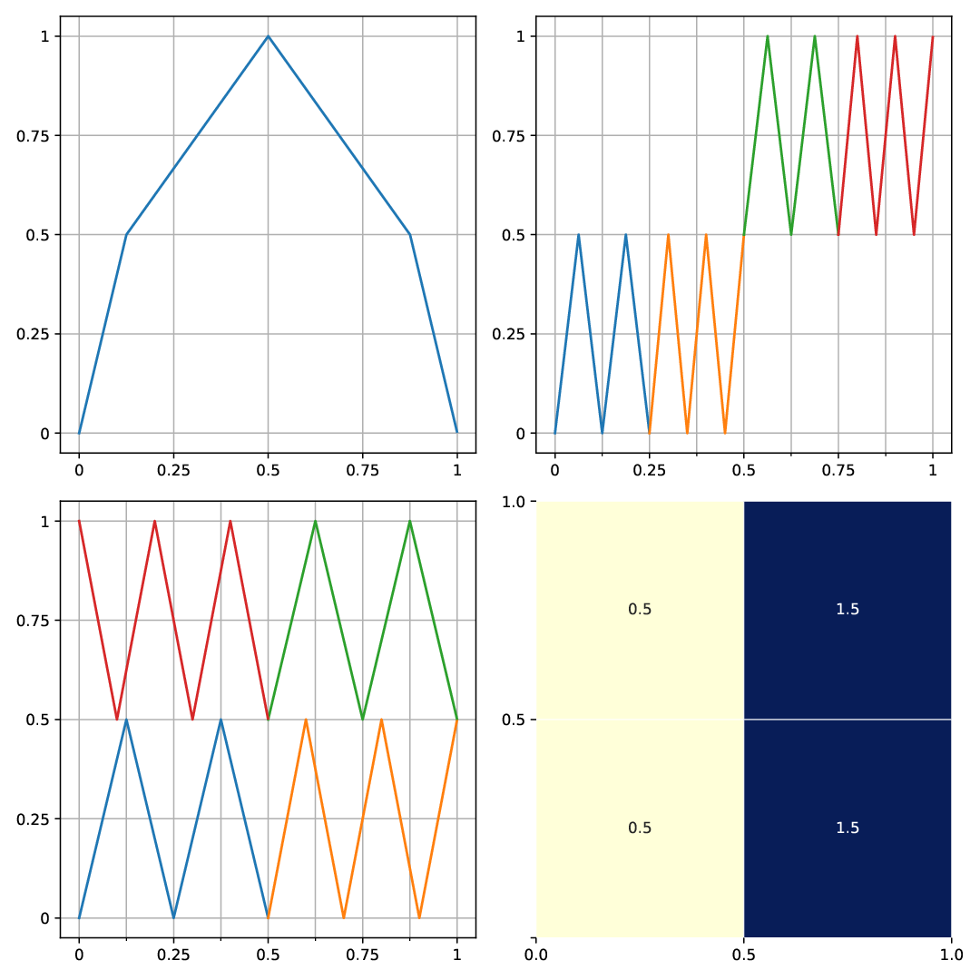
The transport map realized by the network in Theorem 4.3 is based on the generalized space-filling construction $f(g_{s}(x))$ , which has “teeth” in the form of $f(x)$ . For an illustration see Figure 1.

Now consider a general histogram distribution $p_{X,Y}(x,y)$ in $\mathcal{E}[0,1]_{n}^{2}$ . We make use of the fact that the marginals and the conditional distributions of a two-dimensional histogram distribution are (one-dimensional) histogram distributions and realize $p_{X,Y}(x,y)$ according to $p_{X,Y}(x,y)=p_{X}(x)\sum_{i=0}^{n-1}p_{Y|X}(y|x\in[i/n,(i+1)/n])$ . The formal statement is as follows.

Theorem 4.4.

For every distribution $p_{X,Y}(x,y)$ in $\mathcal{E}[0,1]_{n}^{2}$ , there exists a $\Psi\in\mathcal{N}_{1,2}$ with connectivity $\mathcal{M}(\Psi)<88(n^{2}+ns)$ and of depth $\mathcal{L}(\Psi)=s+5$ , such that

W(\Phi\#U,p_{X,Y})\leq\frac{2\sqrt{2}}{n2^{s}}.

The transport map realized by the network in Theorem 4.4 effectively implements a weighted sum of localized transport maps according to Theorem 4.3 and corresponding to the marginals $p_{Y}(y|x\in[i/n,(i+1)/n]),i=[[0,n-1]]$ . For an illustration see Figure 2.

We remark that choosing $s\sim n$ , makes the error in Theorem 4.4 decay exponentially in $n$ while the connectivity of the network is in $\mathcal{O}(n^{2})$ ; this behavior is asymptotically optimal as the number of parameters in $\mathcal{E}[0,1]^{2}_{n}$ is of the same order. Moreover, we note that Theorem 4.4 generalizes (Bailey & Telgarsky 2018)[Theorem 2.1] from uniform target distributions to arbitrary ones through the histogram approximation method and the novel space-filling transport map construction developed in the proof of Theorem 4.3. This construction can be interpreted as a transport operator in the sense of optimal transport theory (Peyré & Cuturi 2019; Villani 2008), with the source distribution being one-dimensional and the target-distribution two-dimensional.

5 Higher dimensions

The extension of our main result to target distributions of dimension higher than $2$ follows the same general storyline as our $2$ -D results above, i.e., we approximate the target distribution by a histogram distribution, realize this histogram distribution through a transport map, and then show how this transport map can be implemented by a deep ReLU network. The transport map our extension is based on does not follow as a generalization of that for the 2-D case, but is based on an alternative idea.

Theorem 5.1.

Let $d,n\in\mathbb{N}$ . For every $p_{\mathbf{X}}\in\mathcal{E}[0,1]_{n}^{d}$ , there exists a $\Psi\in\mathcal{N}_{1,d}$ with connectivity $\mathcal{M}(\Psi)\leq 22\cdot 2^{d}(n^{d}+n^{d-1}s)$ and of depth $\mathcal{L}(\Psi)=(d-1)(s+3)+2$ , such that

W(\Psi\#U[0,1],p_{\mathbf{X}})\leq\frac{\sqrt{d}}{n2^{s}}.

The transport map underlying this result is based on the following functions. Let $s\in\mathbb{N}$ , $\Delta=[a,b]\subset[0,1]$ , set $\widetilde{b}=a+\frac{2^{s}(b-a)}{1+2^{s}}$ , and define

g_{s}^{\Delta}(x):=\frac{1}{n}g_{s}\left(\frac{x-a}{b-a}\right),

h_{s}^{\Delta}(x):=g_{s}^{\Delta}\left(\frac{x-a}{\widetilde{b}-a}\right)+\frac{1}{n(b-\widetilde{b})}(\rho(x-\widetilde{b})-\rho(x-b)).

Figure 3: Plots of

g_{s}^{\Delta}(x)

(left) and

h_{s}^{\Delta}(x)

(right) with

n=1,a=0,b=1,s=2

Rather than providing the full details, which are notationally very cumbersome, for illustration purposes, we specify the transport map for the special case $d=2$ and $n=2^{k}$ , for some $k\in\mathbb{N}$ .

Let $p_{X,Y}(x,y)\in\mathcal{E}[0,1]^{2}_{n}$ have weights $w_{\mathbf{k}}$ and denote the piecewise linear function corresponding to the marginal histogram distribution $p_{X}$ according to Theorem 3.3 by $f_{\text{marg}}$ . Note that the marginal histogram has weights $w_{k}=\frac{1}{n}\sum_{i=0}^{n-1}w_{k,i}$ . Let $\Delta_{S_{\mathbf{k}}}:=[\frac{1}{n^{2}}\sum_{\mathbf{y}:S_{\mathbf{y}}<S_{\mathbf{k}}}\frac{w_{\mathbf{y}}}{w_{y_{1}}},\frac{1}{n^{2}}\sum_{\mathbf{y}:S_{\mathbf{y}}\leq S_{\mathbf{k}}}\frac{w_{\mathbf{y}}}{w_{y_{1}}}]$ , where the order relation $S_{\mathbf{y}}<S_{\mathbf{k}}$ is according to the following definition.

Definition 5.2 (Snake ordering).

Let $\mathbf{k},\mathbf{k}^{\prime}\in[[0,n-1]]^{2}$ , with $\mathbf{k}=(x_{1},x_{2}),\mathbf{k}^{\prime}=(x^{\prime}_{1},x^{\prime}_{2})$ be distinct. The snake ordering is defined as follows

•

if $x_{2}<x^{\prime}_{2}$ , then $\mathbf{k}<\mathbf{k}^{\prime}$ ;
•

if $x_{2}=x^{\prime}_{2}$ and $x_{2}\in 2\mathbb{N}_{0}$ , then $\mathbf{k}<\mathbf{k}^{\prime}$ if $x_{1}<x^{\prime}_{1}$ according to the snake ordering;
•

if $x_{2}=x^{\prime}_{2}$ and $x_{2}\in(2\mathbb{N}_{0}+1)$ , then $\mathbf{k}<\mathbf{k}^{\prime}$ if $x_{1}>x^{\prime}_{1}$ according to the snake ordering.

Finally, the transport map is given by

x\rightarrow\bigg(f_{\text{marg}}(g_{k}(x)),\sum_{j=1}^{n}\Big(h_{s}^{\Delta_{jn}}(x)+\sum_{i=1}^{n-1}g_{s}^{\Delta_{i+jn}}(x)\Big)\bigg).

For a corresponding illustration, see Figure 4.

6 Conclusion

The results in this paper show that every $d$ -dimensional Lipschitz-continuous target distribution (under mild conditions on its pdf) can be generated through deep ReLU networks out of a one-dimensional uniform input distribution. What is more, this is possible without incurring a cost—in terms of approximation error measured in Wasserstein-distance—relative to generating the $d$ -dimensional target distribution from $d$ independent random variables. This is accomplished through a two-stage approach, first generating a histogram distribution and then showing that increasing the histogram resolution drives the approximation error to zero while the corresponding network connectivity scales no faster than the number of parameters in the class of histogram distributions considered. Concretely, this means that the generating network we devise has minimum possible connectivity scaling. We finally note that all the constructions in this paper employ histogram distributions of uniform tile size. As deep ReLU networks can generate histogram distributions of general tile sizes, it is likely that the constants in the bounds on the connectivity of the generating networks can be improved.

7 Omitted proofs

7.1 Proof of Theorem 4.3

Proof.

Let $p_{X}(x)$ be the marginal corresponding to $p_{X,Y}(x,y)$ and note that $p_{X}(x)$ is in $\mathcal{E}[0,1]^{1}_{n}$ and has weights $w_{k}$ , $k\in[[0,n-1]]$ . Define the map $M$ as follows $M:[0,1]\rightarrow[0,1]^{2}$ ,

M:x\rightarrow(x,f(g_{s}(x))),

where $g_{s}$ is an $s$ -order sawtooth function according to Equation 2 and $f(x)$ is defined according to Theorem 3.3 such that $f\#U=p_{X}(x)$ . Fix $s\in\mathbb{N}$ , take an arbitrary $r\in[[0,2^{s-1}-1]]$ , and consider $f(g_{s}(x))$ on the interval $P_{r}=[\frac{r}{2^{s-1}},\frac{r+1}{2^{s-1}}]$ . By Lemma 4.2, $f(g_{s}(x))=f(g(2^{s-1}x-r)),\forall x\in P_{r}$ . Now, let $c^{r}_{k,k_{1}}=[r2^{-s+1},(r+1)2^{-s+1}]\times[k/n+k_{1}2^{-s+1}/n,k/n+(k_{1}+1)2^{-s+1}/n]$ , $r,k_{1}\in[[0,2^{s-1}-1]],k\in[[0,n-1]]$ . By Lemma 4.1, we have for all $k_{1},k$ ,

(M\#U(P_{r}))(x\in c^{r}_{k,k_{1}})=p_{X,Y}((x,y)\in c^{r}_{k,k_{1}}).

(3)

Since $p_{X,Y}((x,y)\in c^{r}_{k,k_{1}})=\frac{w_{k}}{n^{2}2^{s-1}}$ , for all $r\in[[0,2^{s-1}-1]]$ , independently of $r$ , by Lemma 4.2, Equation 3 holds for all intervals $P_{r}$ , $r\in[[0,2^{s-1}-1]]$ . We have hence established that for all $r,k,k_{1}$ , the map $M$ distributes probability mass to each of the rectangles $c^{r}_{k,k_{1}}$ according to $p_{X,Y}((x,y)\in c^{r}_{k,k_{1}})$ . We refer to Figure 1 for a visualization of the transport map $M$ . Since $|x-y|\leq 2^{-s+1}\sqrt{1+\frac{1}{n}}\leq 2^{-s+3/2}$ for any two points in a rectangle of dimensions $(2^{-s+1}\times n^{-1}2^{-s+1})$ , there exists a coupling $\pi$ that, in each $c^{r}_{k,k_{1}}$ , associates points between $p_{X,Y}(x,y)$ and $M\#U$ owing to which we have

W(M\#U,p_{X,Y}(x,y))\leq\int_{[0,1]^{2}}2^{-s+3/2}d(x,y)=\frac{2\sqrt{2}}{2^{s}}.

It remains to show how the transport map

x\rightarrow(x,f(g_{s}(x)))

can be realized through a ReLU network.

We start by noting that the function $f(x)=\sum_{i=1}^{n}a_{i}\max\big(0,x-b_{i}\big)$ can be realized through the network $\Phi_{1}\in\mathcal{N}_{1,1}$ with $\Phi_{1}(x)=\sum_{i=1}^{n}a_{i}\rho(x-b_{i})$ , $\mathcal{M}(\Phi_{1})\leq 3n$ , and $\mathcal{L}(\Phi_{1})=2$ . The network $\Psi^{s}_{g}(x)$ realizing $g_{s}(x)$ is in $\mathcal{N}_{1,1}$ with $\mathcal{M}(\Psi^{s}_{g})=11s-3$ and $\mathcal{L}(\Psi^{s}_{g})=s+1$ . It follows by Lemma II.3 in (Elbrächter et al. 2019) that $\Psi^{f}_{s}=\Phi_{1}(\Psi^{s}_{g})$ is in $\mathcal{N}_{1,1}$ , with $\mathcal{M}(\Psi^{f}_{s})\leq 22s+6n-6$ and $\mathcal{L}(\Psi^{f}_{s})=s+3$ . The network $\Phi_{2}(x)=\rho(x)-\rho(-x)=x$ is in $\mathcal{N}_{1,1}$ with $\mathcal{M}(\Phi_{2})=4$ and $\mathcal{L}(\Phi_{2})=2$ . By Lemma II.4 in (Elbrächter et al. 2019), there exists a network $\tilde{\Phi}_{2}(x)=\Phi_{2}(x)$ with $\mathcal{M}(\tilde{\Phi}_{2})\leq 2s+8$ and $\mathcal{L}(\tilde{\Phi}_{2})=s+3$ . Finally, parallelizing $\tilde{\Phi}_{2}$ and $\Psi^{f}_{s}$ using Lemma A.7 in (Elbrächter et al. 2019), we obtain the network $\Psi=(\tilde{\Phi}_{2},\Psi^{f}_{s})$ , $\Psi\in\mathcal{N}_{1,2}$ , with $\mathcal{M}(\Psi)\leq 6n+24s+2$ and $\mathcal{L}(\Psi)=s+3$ , implementing the desired transport map $x\rightarrow(x,f(g_{s}(x)))$ . ∎

7.2 Proof of Theorem 4.4

Proof.

Let $I_{i}=[i/n,(i+1)/n]$ for $i\in[[0,n-1]]$ and let the weights of $p_{X,Y}(x,y)$ be given by $w_{k_{1},k_{2}}$ . Then, for every $i\in[[0,n-1]]$ , consider the distribution $p_{Y}^{i}(y)=p_{Y}(y|x\in[i/n,(i+1)/n])\in\mathcal{E}[0,1]^{1}_{n}$ with weights $w^{i}_{k}=\frac{nw_{i,k}}{\sum_{j=0}^{n-1}w_{j,k}}$ , for $k\in[[0,n-1]]$ , and let $f_{i}(x)$ be the corresponding piecewise linear function according to Theorem 3.3 such that $f_{i}\#U=p_{Y}^{i}$ . It follows from Definition 1.6, by integrating over $y$ , that the marginal $p_{X}(x)\in\mathcal{E}[0,1]^{1}_{n}$ has weights $w_{i}=\sum_{j=0}^{n-1}w_{i,j}/n$ , and we denote the piecewise linear function generating it according to Theorem 3.3 as $f_{\text{marg}}(x)$ , i.e., $f_{\text{marg}}\#U=p_{X}$ . Take an arbitrary $r\in[[0,n-1]]$ , fix $s\in\mathbb{N}$ , and consider the following transport map

M:x\rightarrow\Bigg(f_{\text{marg}}(x),\sum_{i=0}^{n-1}f_{i}(g_{s}(nf_{\text{marg}}(x)-i))\Bigg)

(4)

on the interval $P_{r}:=[\frac{1}{n}\sum_{j=0}^{r-1}w_{j},\frac{1}{n}\sum_{j=0}^{r}w_{j}]$ . For $x\in P_{r}$ , $f_{\text{marg}}(x)\in[r/n,(r+1)/n]$ and by Theorem 3.3 its explicit form is given by $f_{\text{marg}}(x)=\frac{x}{w_{r}}-\frac{\sum_{j=0}^{r-1}w_{j}}{nw_{r}}+\frac{r}{n}$ . Therefore, $(nf_{\text{marg}}(x)-i)\in[r-i,r-i+1]$ and $f_{i}(g_{s}(nf_{\text{marg}}(x)-i))=0$ , when $i\neq r$ , as $g_{s}(x)=0,\forall x\notin[0,1]$ . For $x\in P_{r}$ , the transport map in Equation 4 hence becomes

x\rightarrow\bigg(\frac{x}{w_{r}}-\frac{\sum_{j=0}^{r-1}w_{j}}{nw_{r}}+\frac{r}{n},p_{r}\Big(g_{s}\Big(\frac{nx-\sum_{j=0}^{r-1}w_{j}}{w_{r}}\Big)\Big)\bigg).

Now, let $c^{r,r_{1}}_{k,k_{1}}=[r/n+r_{1}2^{-s+1}/n,r/n+(r_{1}+1)2^{-s+1}/n]\times[k/n+k_{1}2^{-s+1}/n,k/n+(k_{1}+1)2^{-s+1}/n]$ , $r_{1},k_{1}\in[[0,2^{s-1}-1]],k\in[[0,n-1]]$ . The square $c^{r,r_{1}}_{k,k_{1}}$ has area $\frac{2^{-2s+2}}{n^{2}}$ and $p_{X,Y}((x,y)\in c^{r,r_{1}}_{k,k_{1}})=\frac{w_{r,k}}{2^{2s-2}n^{2}}$ . Combining Lemmas 4.1 and 4.2, we obtain that for all $r_{1},k_{1},k$ ,

		$\displaystyle(M\#U(P_{r}))(x\in c^{r,r_{1}}_{k,k_{1}})=\frac{w_{r}}{2^{s-1}n}\cdot\frac{w^{r}_{k}}{2^{s-1}n}$
		$\displaystyle=\frac{\sum_{j=0}^{n-1}w_{r,j}}{2^{2s-2}n^{3}}\cdot\frac{nw_{r,k}}{\sum_{j=0}^{n-1}w_{r,j}}=\frac{w_{r,k}}{2^{2s-2}n^{2}}$
		$\displaystyle=p_{X,Y}((x,y)\in c^{r,r_{1}}_{k,k_{1}}).$

In summary, we found that $(M\#U(P_{r}))(x\in c^{r,r_{1}}_{k,k_{1}})=p_{X,Y}((x,y)\in c^{r,r_{1}}_{k,k_{1}})$ , for arbitrary $r\in[[0,n-1]]$ . This establishes that for all $r,r_{1},k,k_{1}$ , the map $M$ distributes probability mass to each of the squares $c^{r,r_{1}}_{k,k_{1}}$ of area $\frac{2^{-2s+2}}{n^{2}}$ according to $p_{X,Y}((x,y)\in c^{r,r_{1}}_{k,k_{1}})$ . We refer to Figure 2 for a visualization of the corresponding transport map $M$ .

Since $|x-y|\leq 2^{-s+3/2}/n$ for any two points in a box of size $(n^{-1}2^{-s+1}\times n^{-1}2^{-s+1})$ , it follows that there exists a coupling $\pi$ between $p_{X,Y}(x,y)$ and $M\#U$ owing to which

W(M\#U,p_{X,Y}(x,y))\leq\frac{2\sqrt{2}}{n2^{s}}.

It remains to devise a ReLU network realizing the transport map in Equation 4.

The functions $f_{i}(x)$ can be implemented through networks $\Phi^{i}_{1}\in\mathcal{N}_{1,1}$ with $\Phi^{i}_{1}(x)=\sum_{\ell=1}^{n}a_{\ell}\rho(x-b_{\ell})$ , $\mathcal{M}(\Phi^{i}_{1})\leq 3n$ , and $\mathcal{L}(\Phi^{i}_{1})=2$ . We then note that $f_{\text{marg}}(x)$ can be realized through a network $\Phi_{2}\in\mathcal{N}_{1,1}$ with $\mathcal{M}(\Phi_{2})\leq 3n$ and $\mathcal{L}(\Phi_{2})=2$ . The networks $\Phi^{i}_{2}(x)$ implementing $nf_{\text{marg}}(x)-i$ are in $\mathcal{N}_{1,1}$ and have $\mathcal{M}(\Phi^{i}_{2})\leq 4n$ , $\mathcal{L}(\Phi^{i}_{2})=2$ , and the network $\Psi^{s}_{g}(x)=g_{s}(x)$ is in $\mathcal{N}_{1,1}$ with $\mathcal{M}(\Psi^{s}_{g})=11s-3$ and $\mathcal{L}(\Psi^{s}_{g})=s+1$ . By Lemma II.3 in (Elbrächter et al. 2019), it follows that the networks $\Psi^{i}_{s}=\Phi^{i}_{1}(\Psi^{s}_{g}(\Phi^{i}_{2}))$ are in $\mathcal{N}_{1,1}$ with $\mathcal{M}(\Psi^{i}_{s})\leq 20n+44s-12$ and $\mathcal{L}(\Psi^{i}_{s})=s+5$ . By Lemma II.6 in (Elbrächter et al. 2019), the network $\Psi^{\Sigma}=\sum_{i=0}^{n-1}\Psi^{i}_{s}$ realizing $\sum_{i=0}^{n-1}f_{i}\Big(g_{s}\Big(nf_{\text{marg}}(x)-i\Big)\Big)$ is in $\mathcal{N}_{1,1}$ with $\mathcal{M}(\Psi^{\Sigma})\leq 20n^{2}+44ns-12$ and $\mathcal{L}(\Psi^{\Sigma})=s+5$ . Thanks to Lemma II.4 in (Elbrächter et al. 2019), there exists a network $\tilde{\Phi}_{2}(x)=\Phi_{2}(x)$ in $\mathcal{N}_{1,1}$ with $\mathcal{M}(\tilde{\Phi}_{2})\leq 4n+2s+6$ and $\mathcal{L}(\tilde{\Phi}_{2})=s+5$ . Parallelizing $\tilde{\Phi}_{2}$ and $\Psi^{\Sigma}$ using Lemma A.7 in (Elbrächter et al. 2019), we obtain the network $\Psi=(\tilde{\Phi}_{2},\Psi^{\Sigma})$ , $\Psi\in\mathcal{N}_{1,2}$ , with $\mathcal{M}(\Psi)\leq 20n^{2}+44ns+4n+2s-6<88(n^{2}+ns)$ and $\mathcal{L}(\Psi)=s+5$ , and realizing the transport map

x\rightarrow\Bigg(f_{\text{marg}}(x),\sum_{i=0}^{n-1}f_{i}\Big(g_{s}\Big(nf_{\text{marg}}(x)-i)\Big)\Big)\Bigg).\qed

References

Bailey & Telgarsky (2018) Bailey, B. and Telgarsky, M. J. Size-noise tradeoffs in generative networks. In Bengio, S., Wallach, H., Larochelle, H., Grauman, K., Cesa-Bianchi, N., and Garnett, R. (eds.), Advances in Neural Information Processing Systems 31, pp. 6489–6499. Curran Associates, Inc., 2018. URL https://arxiv.org/abs/1810.11158.
Barron (1993) Barron, A. R. Universal approximation bounds for superpositions of a sigmoidal function. IEEE Transactions on Information Theory, 39(3):930–945, May 1993. ISSN 1557-9654. doi: 10.1109/18.256500. URL https://ieeexplore.ieee.org/document/256500.
Bowman et al. (2016) Bowman, S. R., Vilnis, L., Vinyals, O., Dai, A., Jozefowicz, R., and Bengio, S. Generating sentences from a continuous space. In Proceedings of The 20th SIGNLL Conference on Computational Natural Language Learning, pp. 10–21, Berlin, Germany, August 2016. Association for Computational Linguistics. doi: 10.18653/v1/K16-1002. URL https://www.aclweb.org/anthology/K16-1002.
Box & Muller (1958) Box, G. E. P. and Muller, M. E. A note on the generation of random normal deviates. Ann. Math. Statist., 29(2):610–611, 06 1958. doi: 10.1214/aoms/1177706645. URL https://doi.org/10.1214/aoms/1177706645.
Clement & Desch (2008) Clement, P. and Desch, W. An elementary proof of the triangle inequality for the Wasserstein metric. Proceedings of the American Mathematical Society - PROC AMER MATH SOC, 136:333–340, 01 2008. doi: 10.1090/S0002-9939-07-09020-X. URL https://www.ams.org/journals/proc/2008-136-01/S0002-9939-07-09020-X/.
Devroye (1986) Devroye, L. Sample-based non-uniform random variate generation. In Proceedings of the 18th Conference on Winter Simulation, WSC ’86, pp. 260–265, New York, NY, USA, 1986. Association for Computing Machinery. ISBN 0911801111. doi: 10.1145/318242.318443. URL https://doi.org/10.1145/318242.318443.
Elbrächter et al. (2019) Elbrächter, D., Perekrestenko, D., Grohs, P., and Bölcskei, H. Deep neural network approximation theory. IEEE Transactions on Information Theory, 2019. URL http://www.mins.ee.ethz.ch/pubs/p/deep-it-2019. submitted.
Gibbs & Su (2002) Gibbs, A. L. and Su, F. E. On choosing and bounding probability metrics. International Statistical Review, 70(3):419–435, 2002. doi: 10.1111/j.1751-5823.2002.tb00178.x. URL https://onlinelibrary.wiley.com/doi/abs/10.1111/j.1751-5823.2002.tb00178.x.
Goodfellow et al. (2014) Goodfellow, I., Pouget-Abadie, J., Mirza, M., Xu, B., Warde-Farley, D., Ozair, S., Courville, A., and Bengio, Y. Generative adversarial nets. In Ghahramani, Z., Welling, M., Cortes, C., Lawrence, N. D., and Weinberger, K. Q. (eds.), Advances in Neural Information Processing Systems 27, pp. 2672–2680. Curran Associates, Inc., 2014. URL http://papers.nips.cc/paper/5423-generative-adversarial-nets.pdf.
Karras et al. (2019) Karras, T., Laine, S., and Aila, T. A style-based generator architecture for generative adversarial networks. 2019 IEEE/CVF Conference on Computer Vision and Pattern Recognition (CVPR), pp. 4396–4405, 2019. URL https://arxiv.org/abs/1812.04948.
Kingma & Welling (2014) Kingma, D. and Welling, M. Auto-encoding variational bayes. Proceedings of the 2nd International Conference on Learning Representations (ICLR), 2014. URL https://arxiv.org/abs/1312.6114.
Lee et al. (2017) Lee, H., Ge, R., Ma, T., Risteski, A., and Arora, S. On the ability of neural nets to express distributions. In Kale, S. and Shamir, O. (eds.), Proceedings of the 30th Conference on Learning Theory, COLT 2017, Amsterdam, The Netherlands, 7-10 July 2017, volume 65 of Proceedings of Machine Learning Research, pp. 1271–1296. PMLR, 2017. URL http://proceedings.mlr.press/v65/lee17a.html.
Lu & Lu (2020) Lu, Y. and Lu, J. A universal approximation theorem of deep neural networks for expressing distributions. arXiv preprint arXiv:2004.08867, 2020. URL https://arxiv.org/abs/2004.08867.
Peyré & Cuturi (2019) Peyré, G. and Cuturi, M. Computational optimal transport. Foundations and Trends in Machine Learning, 11(5-6):355–607, 2019. ISSN 1935-8237. doi: 10.1561/2200000073. URL http://dx.doi.org/10.1561/2200000073.
Radford et al. (2016) Radford, A., Metz, L., and Chintala, S. Unsupervised representation learning with deep convolutional generative adversarial networks. In Bengio, Y. and LeCun, Y. (eds.), 4th International Conference on Learning Representations, ICLR 2016, San Juan, Puerto Rico, May 2-4, 2016, Conference Track Proceedings, 2016. URL http://arxiv.org/abs/1511.06434.
Telgarsky (2016) Telgarsky, M. Benefits of depth in neural networks. In Feldman, V., Rakhlin, A., and Shamir, O. (eds.), 29th Annual Conference on Learning Theory, volume 49 of Proceedings of Machine Learning Research, pp. 1517–1539, Columbia University, New York, New York, USA, 23–26 Jun 2016. PMLR. URL http://proceedings.mlr.press/v49/telgarsky16.html.
Tolstikhin et al. (2018) Tolstikhin, I., Bousquet, O., Gelly, S., and Schölkopf, B. Wasserstein auto-encoders. In 6th International Conference on Learning Representations (ICLR), May 2018. URL https://openreview.net/forum?id=HkL7n1-0b.
Villani (2008) Villani, C. Optimal transport: Old and new, volume 338. Springer Science & Business Media, 2008. URL https://www.springer.com/de/book/9783540710493.
Xu et al. (2018) Xu, J., Ren, X., Lin, J., and Sun, X. Diversity-promoting GAN: A cross-entropy based generative adversarial network for diversified text generation. In Proceedings of the 2018 Conference on Empirical Methods in Natural Language Processing, pp. 3940–3949, Brussels, Belgium, October-November 2018. Association for Computational Linguistics. doi: 10.18653/v1/D18-1428. URL https://www.aclweb.org/anthology/D18-1428.