Verification of Initial-State Opacity for Switched Systems: A Compositional Approach

There have been some recent attempts to extend the notion of opacity to continuous-space dynamical systems [5, 6, 7, 8]. In [5], a framework for opacity was introduced for the class of discrete-time linear systems, where the notion of opacity was formulated as an output reachability property rather than an information-flow one. The results in [6] presented a formulation of opacity-preserving (bi)simulation relations between transition systems, which allows one to verify opacity of an infinite-state transition system by leveraging its associated finite quotient one. However, the notion of opacity proposed in this work assumes that the outputs of systems are symbols and are exactly distinguishable from each other, thus, is only suitable for systems with purely logical output sets. In a more recent paper [7], a new notion of approximate opacity was proposed to accommodate imperfect measurement precision of intruders. Based on this, the authors proposed a notion of so-called approximate opacity-preserving simulation relation to capture the closeness between continuous-space systems and their finite abstractions (a.k.a symbolic models) in terms of preservation of approximate opacity. The recent results in [8] investigated opacity for discrete-time stochastic control systems using a notion of so-called initial-state opacity-preserving stochastic simulation functions between stochastic control systems and their finite abstractions (a.k.a. finite Markov decision processes).

Although the results in [6, 7, 8] look promising, the computational complexity of the construction of finite abstractions in those works grows exponentially with respect to the dimension of the state set, and, hence, those existing approaches will become computationally intractable when dealing with large-scale systems.

Motivated by those abstraction-based techniques in [6, 7, 8] and their limitations, this work proposes an approach to analyze approximate initial-state opacity for networks of switched systems by constructing their opacity-preserving finite abstractions compositionally. There have been some recent results proposing compositional techniques for constructing finite abstractions for networks of systems (see the results in [9, 10, 11, 12, 13] for more details). However, the aforementioned compositional schemes are proposed for the sake of controller synthesis for temporal logic properties, and none of them are applicable to deal with security properties including opacity.

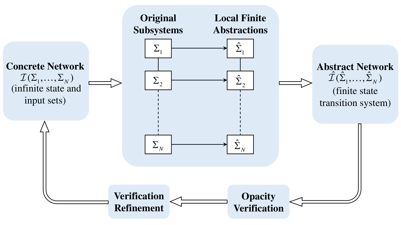
In this paper, we provide for the first time a compositional approach to analyze approximate initial-state opacity of a network of switched systems using their finite abstractions. A new notion of so-called approximate initial-state opacity-preserving simulation function (InitSOPSF) is introduced as a system relation to characterize the closeness between two networks in terms of preservation of approximate initial-state opacity. We show that such an InitSOPSF can be established by composing certain local InitSOPSFs which relate each switched subsystem to its local finite abstraction. Moreover, under some assumptions ensuring incremental input-to-state stability of discrete-time switched systems, an approach is provided to construct local finite abstractions along with the corresponding local InitSOPSFs for all of the subsystems. Then, we derive some small-gain type conditions, under which one can construct a finite abstraction of the concrete network of switched systems by interconnecting local finite abstractions of subsystems. Finally, one can leverage the constructed finite abstraction of the network to check its opacity. The proposed compositional abstraction-based opacity verification pipeline is depicted in Figure 1.

The rest of this paper is organized as follows. In Section 2, we first introduce necessary notations and preliminaries of the paper. Then, a new notion of approximate opacity preserving simulation functions (InitSOPSFs) is proposed in Section 3. In Section 4, we provide a compositional framework for the construction of InitSOPSF for a network of discrete-time switched systems. In Section 5, we present how to construct local finite abstractions for a class of incrementally input-to-state stable subsystems, and then propose a small-gain type condition required for the main compositionality result. Next, an illustrative example is provided in Section 6 that showcases how one can leverage our compositionality results for the verification of opacity for a network of switched systems. Finally, we conclude the paper in Section 7.

We denote by $\mathbb{R}$ and $\mathbb{N}$ the set of real numbers and non-negative integers, respectively. These symbols are annotated with subscripts to restrict them in the obvious way, e.g. $\mathbb{R}_{>0}$ denotes the positive real numbers. We denote the closed, open, and half-open intervals in $\mathbb{R}$ by $[a,b]$, $(a,b)$, $[a,b)$, and $(a,b]$, respectively. For $a,b\in\mathbb{N}$ and $a\leq b$, we use $[a;b]$, $(a;b)$, $[a;b)$, and $(a;b]$ to denote the corresponding intervals in $\mathbb{N}$. Given any $a\in\mathbb{R}$, $|a|$ denotes the absolute value of $a$. Given $N\in\mathbb{N}_{\geq 1}$ vectors $\nu_{i}\in\mathbb{R}^{n_{i}}$, $n_{i}\in\mathbb{N}_{\geq 1}$, and $i\in[1;N]$, we use $\nu=[\nu_{1};\ldots;\nu_{N}]$ to denote the vector in $\mathbb{R}^{n}$ with $n=\sum_{i}n_{i}$ consisting of the concatenation of vectors $\nu_{i}$. Moreover, $\|\nu\|$ denotes the infinity norm of $\nu$. The individual elements in a matrix $A\in\mathbb{R}^{m\times n}$, are denoted by $\{A\}_{i,j}$, where $i\in[1;m]$ and $j\in[1;n]$. We denote by $\text{card}(\cdot)$ the cardinality of a given set and by $\emptyset$ the empty set. For any set $S\subseteq\mathbb{R}^{n}$ of the form of finite union of boxes, e.g., $S=\bigcup_{j=1}^{M}S_{j}$ for some $M\in\mathbb{N}$, where $S_{j}=\prod_{i=1}^{n}[c_{i}^{j},d_{i}^{j}]\subseteq\mathbb{R}^{n}$ with $c^{j}_{i}<d^{j}_{i}$, we define $\emph{span}(S)=\min_{j=1,\ldots,M}\eta_{S_{j}}$ and $\eta_{S_{j}}=\min\{|d_{1}^{j}-c_{1}^{j}|,\ldots,|d_{n}^{j}-c_{n}^{j}|\}$. Moreover, for a set in the form of $X=\prod_{i=1}^{N}X_{i}$, where $X_{i}\subseteq\mathbb{R}^{n_{i}}$, $\forall i\in[1;N]$, are of the form of finite union of boxes, and any positive (component-wise) vector $\phi=[\phi_{1};\dots;\phi_{N}]$ with $\phi_{i}\leq\emph{span}(X_{i})$, $\forall i\in[1;N]$, we define $[X]_{\phi}=\prod_{i=1}^{N}[X_{i}]_{\phi_{i}}$, where $[X_{i}]_{\phi_{i}}=[\mathbb{R}^{n_{i}}]_{\phi_{i}}\cap{X_{i}}$ and $[\mathbb{R}^{n_{i}}]_{\phi_{i}}=\{a\in\mathbb{R}^{n_{i}}\mid a_{j}=k_{j}\phi_{i},k_{j}\in\mathbb{Z},j=1,\ldots,n_{i}\}$. Note that if $\phi=[\eta;\dots;\eta]$, where $0<\eta\leq\emph{span}(S)$, we simply use notation $[S]_{\eta}$ rather than $[S]_{\phi}$. With a slight abuse of notation, we write $[S]_{0}:=S$. Note that $[S]_{\eta}\neq\emptyset$ for any $0\leq\eta\leq\emph{span}(S)$. We use notations $\mathcal{K}$ and $\mathcal{K}_{\infty}$ to denote different classes of comparison functions, as follows: $\mathcal{K}=\{\alpha:\mathbb{R}_{\geq 0}\rightarrow\mathbb{R}_{\geq 0}|$ $\alpha$ is continuous, strictly increasing, and $\alpha(0)=0\}$; $\mathcal{K}_{\infty}=\{\alpha\in\mathcal{K}|$ $\lim\limits_{r\rightarrow\infty}\alpha(r)=\infty\}$. For $\alpha,\gamma\in\mathcal{K}_{\infty}$ we write $\alpha\leq\gamma$ if $\alpha(r)\leq\gamma(r)$, and, with abuse of the notation, $\alpha=c$ if $\alpha(r)=cr$ for all $c,r\geq 0$. Finally, we denote by $\mathcal{I}_{d}$ the identity function over $\mathbb{R}_{\geq 0}$, that is $\mathcal{I}_{d}(r)=r,\forall r\in\mathbb{R}_{\geq 0}$. Given sets $X$ and $Y$ with $X\subset Y$, the complement of $X$ with respect to $Y$ is defined as $Y\backslash X=\{x:x\in Y,x\notin X\}.$

We consider discrete-time switched systems of the following form.

Let $\varphi_{k},k\in\mathbb{N}_{\geq 1}$, denote the time when the $k$-th switching instant occurs. We assume that signal $\mathsf{p}$ satisfies a dwell-time condition [14] (i.e. there exists $k_{d}\in\mathbb{N}_{\geq 1}$, called the dwell-time, such that for all consecutive switching time instants $\varphi_{k},\varphi_{k+1}$, $\varphi_{k+1}-\varphi_{k}\geq k_{d}$). If for all $x\in\mathbb{X},p\in P,w\in\mathbb{W}$, $\text{card}(f_{p}(x,w))\leq 1$, we say the system $\Sigma$ is deterministic, and non-deterministic otherwise. System $\Sigma$ is called finite if $\mathbb{X},\mathbb{W}$ are finite sets and infinite otherwise. Furthermore, if for all $x\in\mathbb{X}$ there exist $p\in P$ and $w\in W$ such that $\text{card}(f_{p}(x,w))\neq 0$ we say the system is non-blocking. In this paper, we only deal with non-blocking systems.

In this subsection, we employ the notion of transition systems, introduced in [15], to provide an alternative description of switched systems that can be later directly related to their finite abstractions in a common framework.

Note that in the above definition, two additional variables $p$ and $l$ are added to the state tuple of the system $\Sigma$. The variable $p$ captures whether or not a switching is allowed for the system at a given time instant, and $l$ serves as a memory to record the sojourn of switching signal.

The following proposition is borrowed from [13] showing that the output runs of a dt-SS $\Sigma$ and its associated transition system $T(\Sigma)$ are equivalent so that one can use $\Sigma$ and $T(\Sigma)$ interchangeably.

Next, let us introduce a formal definition of networks of dt-SS (or equivalently, networks of transition systems).

Consider $N\in\mathbb{N}_{\geq 1}$ dt-SS $\Sigma_{i}=(\mathbb{X}_{i},\mathbb{X}_{0_{i}},\mathbb{X}_{s_{i}},P_{i},\mathbb{W}_{i},$ $F_{i},\mathbb{Y}_{i},h_{i})$, $i\in[1;N]$, with partitioned internal inputs and outputs as

with $w_{ij}\in\mathbb{W}_{ij}$, and $y_{ij}=h_{ij}(x_{i})\in\mathbb{Y}_{ij}$. The outputs $y_{ii}$ are considered as external ones, whereas $y_{ij}$ with $i\neq j$ are interpreted as internal ones which are used to construct interconnections between systems. In particular, we assume that $w_{ij}=y_{ji}$, if there is connection from system $\Sigma_{j}$ to $\Sigma_{i}$, otherwise, we set $h_{ji}\equiv 0$. In the sequel, we denote by $\mathcal{N}_{i}=\{j\in[1;N],j\neq i|h_{ji}\neq 0\}$ the collection of neighboring systems $\Sigma_{j},j\in\mathcal{N}_{i}$, that provide internal inputs to system $\Sigma_{i}$.

Now, we are ready to provide a formal definition of the concrete network consisting of $N\in\mathbb{N}_{\geq 1}$ dt-SS.

Similarly, given transition systems $T(\Sigma_{i})$, one can also define a network of transition systems $\mathcal{I}(T(\Sigma_{1}),\!\ldots\!,T(\Sigma_{N}))$. For the rest of the paper, we mainly deal with the transition systems as they allow us to model dt-SS $\Sigma$ and their finite abstractions in a common framework.

For an interconnection of $N\in\mathbb{N}_{\geq 1}$ finite dt-SS $\hat{\Sigma}_{i}$, with input-output structure configuration as in (3) and (4), we introduce the following definition of networks of finite dt-SS.

Similarly, given finite transition systems $T(\hat{\Sigma}_{i})$, one can also define a network of transition systems as $\hat{\mathcal{I}}(T(\hat{\Sigma}_{1}),\ldots,T(\hat{\Sigma}_{N}))$.

An example of a concrete network and an abstract network is illustrated in Figure 2, where each consists of three switched subsystems.

Before introducing the notion of approximate initial-state opacity for networks of transition systems, we introduce some notations that will be used to characterize opacity property. Consider network $T(\Sigma)$. We use $z^{k}$ to denote the state of $T(\Sigma)$ reached at time $k\in\mathbb{N}$ from initial state $z^{0}$ under an input sequence ${\bar{u}}$ with length $k$, and denote by $\{z^{0},z^{1},\dots,z^{n}\}$ a finite state run of $T(\Sigma)$ with length $n\in\mathbb{N}$.

Here, let us review a notion of approximate initial-state opacity [7]. In this context, the system’s behaviors are assumed to be observed by an outside intruder which aims at inferring secret information of the system. The adopted concept of secrets are formulated as state-based.

Intuitively, the notion of $\delta$-approximate initial-state opacity requires that, whenever observing any output run, an intruder with measurement precision $\delta$ is never certain that the system is initiated from a secret state. In other words, the systems’ secret information can never be revealed in the presence of an intruder that does not have an enough measurement precision.

Suppose that we are given $N$ dt-SS $\Sigma_{i}=(\mathbb{X}_{i},\mathbb{X}_{0_{i}},\mathbb{X}_{s_{i}},P_{i},\mathbb{W}_{i},F_{i},\mathbb{Y}_{i},h_{i})$, $i\in[1;N]$, or equivalently, $T(\Sigma_{i})=(X_{i},X_{0_{i}},X_{s_{i}},U_{i},W_{i},\mathcal{F}_{i},$ $Y_{i},\mathcal{H}_{i})$. Moreover, we assume that each system $T(\Sigma_{i})$ and its abstraction $T(\hat{\Sigma}_{i})$ admit a local $\varepsilon_{i}$-InitSOPSF as defined next.

Note that the local $\varepsilon_{i}$-InitSOPSFs are mainly proposed for constructing a $\varepsilon$-InitSOPSF for the networks and they are not directly used for deducing approximate initial-state opacity-preserving simulation relation. Next, we show how to compose the above defined local $\varepsilon_{i}$-InitSOPSFs so that it can be used to quantify the distance between two networks.

In this subsection, we provide one of the main results of the paper. The following theorem provides a compositional approach for the construction of an $\varepsilon$-InitSOPSF from $T(\Sigma)$ to $T(\hat{\Sigma})$ via local $\varepsilon_{i}$-InitSOPSFs from $T(\Sigma_{i})$ to $T(\hat{\Sigma}_{i})$.

References

• [1] A. Cardenas, S. Amin, B. Sinopoli, A. Giani, A. Perrig et al., “Challenges for securing cyber physical systems,” in Workshop on future directions in cyber-physical systems security, vol. 5, 2009.
• [2] Y. Ashibani and Q. H. Mahmoud, “Cyber physical systems security: Analysis, challenges and solutions,” Computers & Security, vol. 68, pp. 81–97, 2017.
• [3] L. Mazaré, “Using unification for opacity properties,” in IN PROCEEDINGS OF THE WORKSHOP ON ISSUES IN THE THEORY OF SECURITY (WITS’04), 2004, pp. 165–176.
• [4] S. Lafortune, F. Lin, and C. N. Hadjicostis, “On the history of diagnosability and opacity in discrete event systems,” Annual Reviews in Control, vol. 45, pp. 257–266, 2018.
• [5] B. Ramasubramanian, W. R. Cleaveland, and S. Marcus, “Notions of centralized and decentralized opacity in linear systems,” IEEE Transactions on Automatic Control, 2019.
• [6] K. Zhang, X. Yin, and M. Zamani, “Opacity of nondeterministic transition systems: A (bi) simulation relation approach,” IEEE Transactions on Automatic Control, vol. 64, no. 12, pp. 5116–5123, 2019.
• [7] X. Yin, M. Zamani, and S. Liu, “On approximate opacity of cyber-physical systems,” IEEE Transactions on Automatic Control, accepted and in press, 2020.
• [8] S. Liu, X. Yin, and M. Zamani, “On a notion of approximate opacity for discrete-time stochastic control systems,” in American Control Conference, 2020, accepted.
• [9] P. J. Meyer, A. Girard, and E. Witrant, “Compositional abstraction and safety synthesis using overlapping symbolic models,” IEEE Transactions on Automatic Control, vol. 63, no. 6, pp. 1835–1841, 2017.
• [10] G. Pola, P. Pepe, and M. D. D. Benedetto, “Symbolic models for networks of control systems,” IEEE Transactions on Automatic Control, vol. 61, no. 11, pp. 3663–3668, 2016.
• [11] A. Swikir and M. Zamani, “Compositional synthesis of finite abstractions for networks of systems: A small-gain approach,” Automatica, vol. 107, no. 11, pp. 551 – 561, 2019.
• [12] K. Mallik, A. Schmuck, S. Soudjani, and R. Majumdar, “Compositional synthesis of finite-state abstractions,” IEEE Transactions on Automatic Control, vol. 64, no. 6, pp. 2629–2636, 2019.
• [13] A. Swikir and M. Zamani, “Compositional synthesis of symbolic models for networks of switched systems,” IEEE Control Systems Letters, vol. 3, no. 4, pp. 1056–1061, 2019.
• [14] D. Liberzon, Switching in Systems and Control. Birkhäuser Basel, 2003.
• [15] A. Swikir and M. Zamani, “Compositional abstractions of interconnected discrete-time switched systems,” in 2019 18th European Control Conference (ECC), 2019, pp. 1251–1256.
• [16] X. Yin and S. Lafortune, “A new approach for the verification of infinite-step and k-step opacity using two-way observers,” Automatica, vol. 80, pp. 162–171, 2017.
• [17] A. Saboori and C. N. Hadjicostis, “Verification of initial-state opacity in security applications of discrete event systems,” Information Sciences, vol. 246, pp. 115–132, 2013.
• [18] D. N. Tran, B. S. Rüffer, and C. M. Kellett, “Incremental stability properties for discrete-time systems,” in Proceedings of the 55th Conference on Decision and Control, 2016, pp. 477–482.
• [19] L. Vu, D. Chatterjee, and D. Liberzon, “Input-to-state stability of switched systems and switching adaptive control,” Automatica, vol. 43, no. 4, pp. 639 – 646, 2007.
• [20] M. Zamani, P. Mohajerin Esfahani, R. Majumdar, A. Abate, and J. Lygeros, “Symbolic control of stochastic systems via approximately bisimilar finite abstractions,” IEEE Transactions on Automatic Control, vol. 59, no. 12, pp. 3135–3150, 2014.
• [21] S. Dashkovskiy, B. Rüffer, and F. Wirth, “Small gain theorems for large scale systems and construction of iss lyapunov functions,” SIAM Journal on Control and Optimization, vol. 48, no. 6, pp. 4089–4118, 2010.
• [22] B. C. Eaves, “Homotopies for computation of fixed points,” Mathematical Programming, vol. 3, no. 1, pp. 1–22, 1972.
• [23] B. S. Ruffer, “Monotone dynamical systems, graphs, and stability of largescale interconnected systems,” Ph.D. thesis, Fachbereich 3, Mathematik und Informatik, Universität Bremen, Germany, 2007.
• [24] Z.-P. Jiang, I. M. Mareels, and Y. Wang, “A lyapunov formulation of the nonlinear small-gain theorem for interconnected iss systems,” Automatica, vol. 32, no. 1, pp. 1211 – 1215, 1996.
• [25] A. Saboori and C. N. Hadjicostis, “Notions of security and opacity in discrete event systems,” in Proceedings of the 46th IEEE Conference on Decision and Control, 2007, pp. 5056–5061.
• [26] ——, “Verification of kk-step opacity and analysis of its complexity,” IEEE Transactions on Automation Science and Engineering, vol. 8, no. 3, pp. 549–559, 2011.
• [27] ——, “Verification of infinite-step opacity and complexity considerations,” IEEE Transactions on Automatic Control, vol. 57, no. 5, pp. 1265–1269, 2012.