An Enhanced Finite Difference Time Domain Method for Two Dimensional Maxwell’s Equations
Abstract.
An enhanced finite-difference time-domain (FDTD) algorithm is built to solve the transverse electric 2D Maxwell’s equations with inhomogeneous dielectric media where the electric fields are discontinuous across the dielectric interface. The new algorithm is derived based upon the integral version of the Maxwell’s equations as well as the relationship between the electric fields across the interface. To resolve the instability issue of Yee’s scheme (staircasing) caused by discontinuous permittivity across the interface, our algorithm revises the permittivities and makes some corrections to the scheme for the cells around the interface. It is also an improvement over the contour-path effective permittivity algorithm by including some extra terms in the formulas. The scheme is validated in solving the scattering of a dielectric cylinder with exact solution from Mie theory and is then compared with the above contour-path method, the usual staircasing and the volume-average method. The numerical results demonstrate that the new algorithm has achieved significant improvement in accuracy over other methods. Furthermore, the algorithm has a simple structure and can be merged into current FDTD software packages easily. The C++ source code for this paper is provided as supporting information for public access.
Key words and phrases:
finite difference time domain; Maxwell’s equations; 2nd order convergence; stability; effective permittivity1. Introduction
The finite-difference time-domain (FDTD) algorithm is one of the most popular numerical methods to solve Maxwell’s equations, as proposed by Yee [1]. It is a time marching forward method which easily makes a visual representation of the fields. It also scales very well since the number of computation required is proportional to the size of the model and the method requires no large-scale linear algebra computation [2]. The FDTD method requires a completely structured grid also known as the Yee grid. However, Many real world problems have complicated geometries and numerical inaccuracy happens when the modeled objects do not fit the grid very well.
In this paper, we focus on two-dimensional transverse electric (TE) Maxwell’s equation within multiple non-magnetic media where the electric fields are not continuous across the media interface so the numerical schemes need to be designed to take care of such discontinuity. The other case is the transverse magnetic equation where the electric field is always continuous across the media interface and the original algorithm will work as in the homogeneous medium.
The original FDTD algorithm proposed in Yee’s paper assigns each of the field component an electric permittivity and a magnetic permeability solely based on the material properties at its location. This is commonly known as the staircasing or pixelation method. In general, the staircasing method has an error that scales with given a grid size of for cells that are homogenous. However, in cells that contain a medium interface, the local error becomes . Even though the number of cells that contain an interface is often a small fraction of the total cells, these local errors can cause a rough global error of .
Subsequent research in modern optics and electromagnetism dealing with the Maxwell’s equations have focused on more and more complex geometries with different materials so that the complicated dielectric tensor can cause serious pixelation issues. In turn, there have been many improvements in FDTD algorithms to overcome these pixelation issues. One way to overcome the pixelation problem is by fitting the mesh to the device, thereby generating the so-called non-orthogonal FDTD [3, 4]. The second method is to refine the Cartesian mesh around the interfaces and is thus called subgridding method [5]. Even though these two methods converge faster than the standard FDTD method, their complexity are larger than original FDTD method and they also have time stability issues.
In order to keep a completely structured grid and maintain all the benefits of FDTD, another method redefines Maxwell’s integral equations around the interface of the media. This is known as the effective-permittivity (EP) method. This method uses sub-pixel smoothing techniques to change the permittivities of the field components around the interface to produce better results by taking account of many different factors, such as the interface conditions, permittivities of adjacent field components and so on. The revised effective permittivities smooth out the pixel error. The main benefit of these methods is that there is a negligible increase of the numerical load since all the revised permittivities have been calculated before the main FDTD algorithm loop.
The first method of sub-pixel smoothing is the volume average effective permittivity (V-EP) [6]. This method assigns effective permittivities for all the field components in a cell that contains media interface. The effective permittivities are calculated by taking a weighted average based on how much percent of the volume each medium occupies. This method is simple for implementation and also stabilizes the error fluctuation that occurs in the staircasing method. However, it does not decrease the error rapidly and its error can be worse than staircasing method sometimes due to ignorance of the interface orientation.
The second method proposes dynamic formulas for the EP based on the orientation of the media interface and their expressions are accurate when the interface is perpendicular or parallel to the mesh axes [7, 8, 9]. These EPs improve the accuracy of the FDTD method, while keeping the simple structure of the original algorithm. However, their performance will deteriorate for a curved or flat interface not perpendicular or parallel to the mesh axes.
The third method uses the reflection coefficients to derive effective permittivities and shows the method can also achieve second-order convergence with several special slanted angles between the interface and the Yee grid rather than just orthogonal or parallel to the Yee grid [10, 11]. However, its derivation is quite complicated and has no ways to be extended to arbitrary interfaces.
In a landmark paper [12], Mohammadi et al. proposed the so-called contour-path effective permittivities (CP-EP) method. The CP-EP method first addresses the orthogonal and parallel cases as shown above, then extends the idea to handle with more general geometry. Unlike the previous methods, it could handle arbitrary boundary with any orientation of the boundary. Compared with traditional staircasing methods, CP-EP has almost no additional runtime cost since determination of the effective permittivities has been done before the main FDTD loop.
However, we will demonstrate that CP-EP does not incorporate one important term from the interface conditions into the FDTD algorithm. Then we will develop a revised EP algorithm where the missing term will be re-considered in order to produce a more accurate and stable algorithm. Since this method incorporates the boundary conditions very well, it will be denoted as BC-EP.
In fact, such deficiency of CP-EP has also been identified in [13, 14] where effective dielectric permittivity tensors are constructed to take care of both isotropic and anisotropic materials so as to achieve second-order convergence under the open source software MEEP. However, such proposed method which satisfies the interface conditions for electromagnetic fields has been shown to have late-time instabilities, and many possibilities to average the effective dielectric tensor are explored to avoid late time instabilities [15]. Further efforts have been reported in [16] to construct a new second-order scheme by taking the average of eight triplets. Although the new method is highly accurate, its effective dielectric permittivity tensor can still be asymmetric thus unstable for certain conditions. Therefore, the last improvement of the effective dielectric tensor has been given in [17] to make it symmetric and stable. The numerical results show that this scheme gives the best result in general and the error in practice still lies in between first and second-order in most cases.
In the following, we will introduce the new BC-EP method by adding a few terms to the established CP-EP method for the cells around the interface so as to keep the numerical load increase as small as possible and improve the accuracy significantly. Then the numerical tests verify that BC-EP has a much better performance than CP-EP, V-EP and staircasing methods while still maintaining numerical stability. BC-EP has a very simple structure and can be merged into any existing FDTD packages easily, compared with other established FDTD software [14, 17] which can be run only within their framework. We provide C++ source code for BC-EP together other three methods as supporting information for public access. Conclusion and some future research consideration will be provided in the end.
2. New Algorithm Design
In this section, we will propose a new effective permittivity method to solve Maxwell’s equations in a domain composed of two different non-magnetic media with different electric permittivities. To simply the algorithm description, we will focus on the most important transverse electric (TE) scenario. That is, is located in the incident xy-plane while is along z-axis. Moreover, we restrict the discussion to dielectric and non-magnetic media such that and where stays as a constant in different media and . Based on the integral version of the Maxwell’s equations, we will derive the new algorithm for any orientation of the interface. This is a significant improvement over all current methods which are only accurate under specific angles between the interface and Cartesian coordinate system, such as parallel or orthogonal to Yee-axis.
As a preliminary step, let us set up the relation of and across the interface of these two media. It is well known that is continuous in the whole domain. Meanwhile, across the media interface, the tangential component of the electric field and the normal component of the electric flux are continuous as well, as shown in Figure 1 where is the outward unit norm vector from region 1.
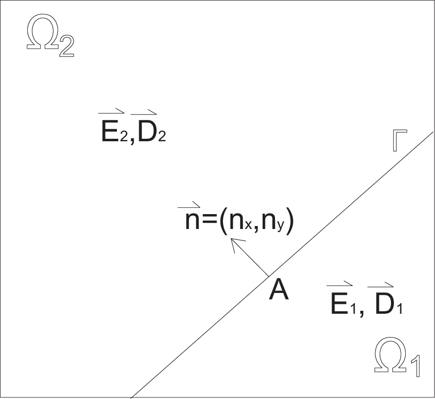
Choose . and are the electric fluxes at A from different media, and and are the corresponding electric fields.
Suppose is the unit norm vector at from region 1, then the corresponding tangent unit vector is Therefore, we can calculate and at point in different regions as follows.
| (1) |
| (2) |
Meanwhile,
| (3) |
| (4) |
Based on the fact that and , we have
Therefore, by using , we get
Or
| (5) |
Furthermore, by using at , we obtain
| (6) |
If the interface is parallel or orthogonal to -axis, either or so . Then the relation (5) involving and will be simplified such that and will only depend on or , respectively. Same holds for and in relation (6).
By using (6), we can express in region 2 based on its neighbor in region 1 and its corresponding in the same region 2. Similar formula can also be derived for based on and .
| (7) | ||||
| (8) |
(5) will be used to derive the new scheme for Faraday’s law while (7) and (8) will be used to derive the new scheme for Ampere’s law.
Now let us express Ampere’s law in integral form
| (9) |
and Faraday’s law integral form
| (10) |
Firstly, let us discretize Ampere’s law (9) around the interface to update and as below.

To update , we choose in (9) to be the rectangle in -plane whose projection in -plane is the line segment . Suppose the interface intersect at point and as in Figure 2. Applying time discretization to Ampere’s law along at time yields
| (11) |
Based on formula (7), we can compute the integrals of left hand side as follows. From now on, all the higher-order terms of and are ignored for the clarification of the formulas.
| (12) |
Similarly,
| (13) |
Furthermore,
| (14) |
By putting (12), (13) and (14) into (11), we obtain
| (15) |
which, based on in , becomes
| (16) |
which shows improved discretization of Ampere’s law for updating
It should also be noted that the last term on the right hand side of (16) have been ignored by CP-EP for algorithm simplification but it indeed provides necessary corrections for the interface conditions across multiple media. Furthermore, the numerical tests have also verified that in order to make the algorithm for Ampere’s Law more accurate, these two values in the last term should stay close to the interface. That is, if the normal direction of the interface satisfies as shown in Figure 2, we use since these two points are closer to the interface, while for the other case, we use in (16) instead since these two nodes are closer to the interface than the other pair. This improvement is feasible since in continuous across the interface.

Similarly, update of at point by Ampere’s law (9) can be taken care analogously as shown in Figure 3, where the interface intersects the line segment , projection of at -plane, at . Let . By repeating the same procedure as above while based on formula (8), we can also obtain the discretization of Ampere’s law for as below:
| (17) |
where in the last term will be replaced by when holds.
Secondly, let’s discretize Faraday’s law (10) around the interface .

We choose to be the rectangle centered at . If the medium interface does not cut through interior of , the standard Yee scheme should apply without modification. So we only consider the case where intersects with . It’s obvious that will only intersect with at most two sides, e.g. the bottom and left side as in Figure 4. All other cases can be handled in the same way. Similarly as for Ampere’s law, all the higher-order terms of dx and dy are ignored for the clarification of the formulas. Discretization of the left hand side term of (10) at the time via finite difference scheme yields
or
| (18) |
since is always perpendicular to the incident -plane and so is always continuous across the interface, then by using midpoint rule,
| (19) |
| (20) |
However, the situation for is much more complicated. In Figure 4, the line integral of along the right and top sides can be handled as Standard Yee scheme since they are completely inside . But the line integrals along the bottom and left sides need to be handled separately.
| (21) |
Suppose the portion OA of the bottom side in has length , and the portion OB of the left side in has length as in Figure 4, then the first two terms on the right hand side of (21) can be handled as below. For the first term on the right hand side of (21), we have
| (22) |
By using formula (5) with and interchanged, we have
| (23) |
Putting it into (22) yields
| (24) |
where is the value of evaluated at point in . However, only instead of is calculated at the mesh point . Therefore, we will take the average value of at the neighboring pair of mesh points and if they are both located within , or take the average value of at the other neighboring pair mesh points and if they are both located within . If none of the pairs are located within , this term will be set to zero as in CP-EP. Therefore, BC-EP will try to make corrections for the missing terms in CP-EP if possible.
Similarly, we can calculate the second term on the right hand side of (21). Since the node is located within instead of , so the new should be negative of the old used above. Therefore, applying integration midpoint rule, Taylor expansion and formula (5) where replaced by and interchanged, we have
| (25) |
when will be taken care similarly as from the first term. By putting (24), (25) into (21), we get
| (26) |
Finally, by putting (19), (20) and (26) into (18) and dividing both sides by , we obtain the new discretization of Faraday’s law:
| (27) |
where the last two terms are expressed by
| and | ||||
If we set in the new algorithm (16), (17) for Amepre’s law and (27) for Faraday’s law, we can retrieve the standard FDTD scheme in homogeneous medium. Therefore, BC-EP is a simple extension of the original schemes in order to take care of the media interface. Meanwhile, the extra terms added in the formulas will greatly improve the accuracy compared with CP-EP. Furthermore, BC-EP has a very simple structure and can be merged into any FDTD software by just revising the effective permittivities and adding some extra terms when necessary.
It should be mentioned that due to complicated expressions of those ignored higher-order terms in the newly derived formulas, it is difficult to demonstrate the convergence order of BC-EP theoretically. However, subsequent numerical results will show that BC-EP can achieve the highest convergence compared with other methods. Another point is that it is still an open challenge to accurately handle objects with sharp corners, where the resulting field singularities are known to degrade the accuracy of all numerical schemes [14]. Therefore, just as other methods, BC-EP performs well for straight or curved interfaces instead of interfaces with corners.
3. Numerical Results
In this section, we will demonstrate convergence order and stability of BC-EP numerically. To accomplish this task, we implement the algorithm to solve the Maxwell’s equations on a dielectric cylinder, together with the staircasing, V-EP, and CP-EP methods. All the implementations are set up for the 2D FDTD TE case. The total scattering cross sections (SCS) are calculated by all four methods and then compared with the well-known analytic solution by Mie Theory [18] so as to measure the accuracy of each method.

The dielectric cylinder is simulated in an area that is times the radius of the cylinder plus some extra space for PML condition. The cylinder is centered at where and are the number of the cells along the and directions, and are the horizontal and vertical mesh sizes of each cell as seen in Figure 5. We run the test for two cases: one case for a larger cylinder with radius and another case for a smaller cylinder with . The total-field/scattered-field line is three times the length of the cylinder radius away from the center, and the integration line for calculating SCS is four times away from the center, while the PML starts at five times away from the center.
The source wave is a planar wave in the direction with a Gaussian envelope , where is six times , is speed of light in a vacuum, and is the testing range of wavelengths. In our simulation, we calculate SCS for wavelengths ranging from to of visual light spectrum with equal distance. Fast Fourier transform (FFT) is then applied to transform the electric and magnetic fields from spatial domain into light frequency domain so as to calculate SCS over all related wavelengths.
We use square unit cells with to simplify the simulation. The time step is set to where to ensure stability [2]. Also for stability concerns, were chosen to divide the smallest tested wave length () by at least twenty times. The total SCS is calculated by using the Poynting Vector along with the integration line as seen in Figure 5. Meanwhile, Mie theory is used to calculate the true value of total SCS for each wavelength. The number of iterations for the main FDTD loop is set large enough in order to give enough time for the electric and magnetic waves to leave the simulated area for stable SCS calculation.


Firstly, we investigate the accuracy and the convergence order of BC-EP and compare it with other similar methods. We test all the methods for a circular cylinder with radius and permittivity . The background media ia always set as air with . The mesh size is originally set to . Each method has been run to calculate the total SCS with different mesh sizes. As seen in (A) of Figure 6, the numerical values from all methods match with the true solution very well. But we can still see that BC-EP has the smallest relative error while V-EP has the largest relative error on most wavelengths shown in (B) of Figure 6. To make a reasonable comparison, for each mesh size , the average relative error of SCS is calculated among all the wavelengths for each method. In order to observe the error convergence order clearly, the average relative errors versus the mesh sizes are converted into a log scale where denotes the log of the number of mesh points for the radius of the cylinder, as seen in Figure 7.

This whole process is then repeated for other larger permittivity values . The numerical results for the average relative errors versus the mesh sizes are reported in Figure 8 for , and in Figure 9 for . Other values have similar outcomes.


It can be seen that BC-EP gives the least amount of error for most cases, followed by CP-EP. Staircasing results are quite erratic and its error doesn’t go down in a uniform manner due to random nature of some mesh sizes conforming with the cylinder better than others. V-EP has the worst error but gives a uniform error decrease with smaller mesh sizes, and thus gives more consistent results over staircasing.
| Permittivity | Staircasing | V-EP | CP-EP | BC-EP |
|---|---|---|---|---|
| 1.6621 | 1.0860 | 1.6977 | 2.4386 | |
| 1.0700 | 1.0850 | 1.4560 | 1.9251 | |
| 1.2160 | 1.1294 | 1.5267 | 1.6974 | |
| 1.3723 | 1.1476 | 1.3607 | 1.5247 | |
| 1.4322 | 1.1834 | 1.3800 | 1.6014 | |
| 1.4283 | 1.1860 | 1.3564 | 1.6423 | |
| 1.4867 | 1.2262 | 1.4333 | 1.6837 | |
| 1.6172 | 1.3183 | 1.5323 | 1.8006 |
To further investigate the order of convergence of all the methods, we estimate the convergence order by computing the slopes from the log figures for all the given permittivity. Table 1 shows BC-EP converges significantly faster than all the other methods. CP-EP is the second in terms of convergence order and outperforms both staircasing and V-EP as demonstrated in [12] already.
To complete the final evaluation of the performance for all the methods, the whole test suite is then repeated for another circular cylinder with smaller radius . All the results are very similar and for brevity, we only report the case of , as seen in Figure 10. It can be seen that BC-EP has a higher convergence order than others. To be more specific, BC-EP, CP-EP, Staircasing and V-EP have the order of convergence , , and , respectively, based on Figure 10.

Therefore, BC-EP is more accurate and converges faster than the other three popular FDTD methods.
Secondly, we investigate the stability of BC-EP since the stability of other methods have been demonstrated in the literature. The algorithm has been run for iterations under FDTD main loop which is long enough for the electric and magnetic waves to leave the region completely. This process has been repeated for and for mesh size and . At every iterations, a calculation of the SCS for all wavelengths is conducted. Then the average relative error between the calculated SCS at that iteration and the exact SCS over those wavelengths is calculated. We observe that the result are very similar for different and different in the sense that the relative errors drop down to zero very quickly, as seen in Figure 11. This shows that there is no electromagnetic power left in the region and the fields return back to zero as excepted, meaning no late time instability even at very high contrast.


4. Conclusions and Future Research
We have built a new BC-EP method for the challenging two-dimensional transverse electric Maxwell’s equations involving multiple dielectric media. Based on a relation for the electric fields across the dielectric media interface and the integral version of the Maxwell’s equations, we derive this method which represents Maxwell’s equations accurately while the previous numerical methods skipped some terms from the boundary conditions for the purpose of algorithm simplification. We then apply BC-EP together with three other popular FDTD methods, CP-EP, staircasing and V-EP, to solve a numerical example of a dielectric cylinder with given analytic solution. The numerical results clearly demonstrate that it always achieves the highest convergence compared with other methods. The stability of BC-EP has also been verified numerically. Due to its simplicity, BC-EP can be merged into other FDTD software packages easily. The C++ source codes for these four methods are provided as supporting information for public access.
References
- [1] Kane Yee, Numerical Solution of Initial Boundary Value Problems Involving Maxwell’s Equations in Isotropic Media, IEEE Transactions on Antennas and Propagation 14, 302–307 (1966).
- [2] Allen Taflove, Susan Hagness, Computational Electrodynamics: The Finite-Difference Time-Domain Method, 3rd Ed. (Artech House, 2005).
- [3] P.H. Harms, J.-F. Lee, R. Mittra, A Study of the Nonorthogonal FDTD Method Versus the Conventional FDTD Technique for Computing Resonant Frequencies of Cylindrical Cavities, IEEE Transactions on Microwave Theory and Techniques 40, 741-746 (1992).
- [4] Jinjie Liu, Moysey Brio, Jerome V. Moloney, Overlapping Yee FDTD Method on Nonorthogonal Grids, Journal of Scientific Computing, 39, 129-143 (2009).
- [5] S.S. Zivanovic, K.S. Yee, K.K. Mei, A Subgridding Method for the Time-Domain Finite-Difference Method to Solve Maxwell’s Equations, IEEE Transactions on Microwave Theory and Techniques (39), 471-479 (1991).
- [6] Supriyo Dey, Raj Mittra, A conformal finite-difference time-domain technique for modeling cylindrical dielectric resonators, IEEE Transactions on Microwave Theory and Techniques 47, 1737–1739 (1999).
- [7] Noriaki Kaneda, Bijan Houshmand, Tatsuo Itoh, FDTD Analysis of Dielectric Resonators with Curved Surfaces, IEEE Transactions on Mircowave Theory and Technique 45, 1645–1648 (1997).
- [8] Kyu-pyung Hwang, Andreas Cangellaris, Effective Permittivities for Second-Order Accurate FDTD Equations at Dielectric Interfaces, IEEE Mircowave and Wireless Components Letters 60, 5259–5267 (2012).
- [9] Dauh-churn Liu, Hung-chun Chang, The Second-order Condition of FDTD Method at Sloped Dielectric Interfaces by Averaging the Permittivities along Surface Normal, IEEE Transactions on Antennas and Propagation 37, 4802–4804 (2012).
- [10] T. Hirono, Y. Shibata, W. Lui, S. Seki, Y. Yoshikuni, The Second-Order Condition for the Dielectric Interface Orthogonal to the Yee-Lattice Axis in the FDTD Scheme, IEEE Mircoewave and Guided Wave Letters 10, 359–361 (2000).
- [11] Takuo Hirono, Yuzo Yoshikuni, Takayuki Yamanaka, Effective permittivities with exact second-order accuracy at inclined dielectric interface for the two-dimensional finite-difference time-domain method, Applied optics 49, 1080–1096 (2010).
- [12] Ahmad Mohammadi, Hamid Nadgaran, Mario Agio, Contour-path effective permittivities for the two-dimensional finite-difference time-domain method, Optics Express 13, 10367–10381 (2005).
- [13] A. Farjadpour, David Roundy, Alejandro Rodriguez, M. Ibanescu, Peter Bermel, J.D. Joannopoulos, Steven Johnson, G.W. Burr, Improving accuracy by subpixel smoothing in the finite-difference time domain, Optics letters 31, 2972–2974 (2006).
- [14] Ardavan Oskooi, Chris Kottke, Steven Johnson, Accurate finite-difference time-domain simulation of anisotropic media by subpixel smoothing, Optics letters 34, 2778–2780 (2009).
- [15] Gregory Werner, John Cary, A stable FDTD algorithm for non-diagonal, anisotropic dielectrics, Journal of Computational Physics 226, 1085–1101 (2007).
- [16] Carl Bauer, Gregory Werner, John Cary, A second-order 3D electromagnetics algorithm for curved interfaces between anisotropic dielectrics on a Yee mesh, Journal of Computational Physics 230, 2060–2075 (2011).
- [17] Gregory Werner, Carl Bauer, John Cary, A more accurate, stable, FDTD algorithm for electromagnetics in anisotropic dielectrics, Journal of Computational Physics 255, 436–455 (2013).
- [18] Craig Bohren, Donald Huffman, Absorption and scattering of light by small particles, (John Wiley and Sons, 1983).
- [19] Ahmad Mohammadi, Tahmineh Jalali, Mario Agio, Dispersive contour-path algorithm for the two-dimensional finite-difference time-domain method, Optics Express 16, 7397–7406 (2008).
- [20] Jinjie Liu, Moysey Brio, Jerome V. Moloney, Subpixel smoothing finite-difference time-domain method for material interface between dielectric and dispersive media, Optics letters 37, 4802–4804 (2012).
- [21] Duc Duy Nguyen, Shan Zhao, A second order dispersive FDTD algorithm for transverse electric Maxwell’s equations with complex interfaces, Computers and Mathematics with Applications 71, 1010–1035 (2016).