Multi-sensory Integration in a Quantum-Like Robot Perception Model
Abstract
Formalisms inspired by Quantum theory have been used in Cognitive Science for decades. Indeed, Quantum-Like (QL) approaches provide descriptive features that are inherently suitable for perception, cognition, and decision processing. A preliminary study on the feasibility of a QL robot perception model has been carried out for a robot with limited sensing capabilities [1]. In this paper, we generalize such a model for multi-sensory inputs, creating a multidimensional world representation directly based on sensor readings. Given a 3-dimensional case study, we highlight how this model provides a compact and elegant representation, embodying features that are extremely useful for modeling uncertainty and decision. Moreover, the model enables to naturally define query operators to inspect any world state, which answers quantifies the robot’s degree of belief on that state.
1 Related Work
Quantum computing has been applied in robotics as a tool for speed up classical tools, or in a framework which is still the classical one [2]. Our approach is quite different: starting from the very properties of quantum systems, we studied how to exploit them in a novel, simpler framework. This approach has been shown effective in quantum perception and cognition modeling, and we argue that this could be extremely useful in Robotics, providing also a way to translate the theoretical models of quantum cognition to practical robotics application. In contrast to the aforementioned research in Quantum Robotics, this approach could be useful even as purely simulated, because its merits are due to quantum system properties rather than merely computational advantages.
Since the early intuitions by Amann [3], quantum cognition research studied the links between perception and quantum dynamics [4, 5, 6, 7]. A relevant example is the work in Manousakis [6], which proposed a QL model to describe probability distributions of perceptive dominances in subjects experiencing binocular rivalry.
A preliminary model inspired by the work in Manousakis [6] has been proposed to assess the feasibility of a QL perception model for a robot with limited sensing capabilities [1]. The reason behind this choice is the great descriptive potential which a quantum formalism inherently provides [8, 9, 10, 11, 12].
Indeed, following Caves et al.[13], quantum probability theory can be understood within the Bayesian approach, with probabilities quantifying the degree of belief about a certain state. In this case, maximal information for a question does not imply complete knowledge, i.e., it does not allow us to predict which state will be measured (which answer will be given) but provides only each state’s probability of being measured (the degree of belief about the possible answers).
This interpretation of the measurement as a query given a certain belief (i.e., the quantum system state) can be extremely useful for decision making [14].
We argue that this interpretation could be adapted with significant results in robot perception and cognition models as well. A QL model provides a way to deal with uncertain perceptual knowledge and decision making without an explicit representation. We posit that this is a more elegant, more compact approach because the state is not a mere vector state as in current thinking. Representing it as a quantum state, we may be capable of leveraging the properties related to measurement and uncertainty in quantum mechanics. Moreover, this approach discloses new perspectives for further investigations. Starting from a QL representation, a wide range of quantum cognition models discussed in the existing literature can be applied to Robotics [9, 10].
The preliminary QL perception model proposed in [1] dealt with one sensory input channel, performing a time integration of the input discriminating between two states. The goal of this study is to generalize such first single-qubit model to a multi-qubit approach. Moreover, exploiting state superposition and a change of basis in the Hilbert space , we can significantly extend the considered states range. Indeed, we can virtually deal with any possible state in 11 1 It is noteworthy that only one query at a time is possible due to the quantum state collapse after any measurement [15]. . To keep the analysis simpler, we do not consider time integration in this paper, although the model may be easily extended to time windows as illustrated for the single-qubit model in [1].
2 Technical Approach
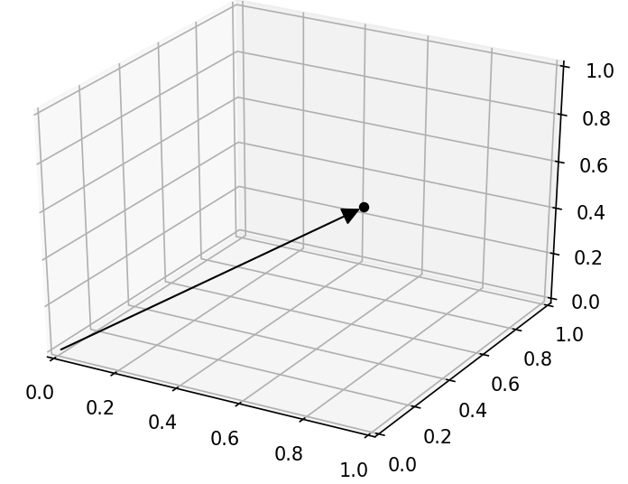

We consider sensors, each one returning a lower- and upper-bounded discrete scalar (Fig. 1). Readings are domain-wise normalized, so the model receives a real value between 0 and 1 for each -th sensor. At each reading update, the model has a vector in input. For example, considering a camera-like sensor able to provide only the three RGB average values of the image, we can decompose it in three sensors, each of them with an interface normalizing the readings in a interval. In this case, the input vector is represented in three dimensions as shown in Fig. 2. Every qubit encodes the sensory information of a corresponding -th sensor. Following [1] we encode sensory data with a unitary operator which applies a rotation to . The main differences with the previous model rely on the multi-qubit generalization, the lack of temporal integration ( for the model proposed here), and the extension to continuous inputs (the previous study assumed being either 0 or 1). Therefore, the information is encoded in the angle of the Bloch sphere representation of , as shown in Fig. 2.
Many indirect methods are available to exploit information encoded in qubits [16]. Here, we consider only state measurements exploiting Caves et al. [13] interpretation, as stated in Section 1. Measuring the quantum system leads to the collapse of its state in one of its basis states, namely the set of states composed by all the ordered combinations of the basis states of each single qubit. The probability for the collapse to produce a certain state as a measurement is given by the current state superposition. For example, considering the input vector we saw in Fig. 2, the overall system state produced by the application of the rotation operators is
| (1) |
As illustrated in Fig. 3, the probability of measuring a certain state is the square of the vector coefficient corresponding to that state. For example, for the -th state 22 2 We use the IBMQ Qiskit [17] notation rather than the one usually used in quantum mechanics. This means that, in the Dirac notation, the states which are normally ordered as are instead ordered as , following the usual bits notation . we have a coefficient and then the probability of measuring it is [15]. These coefficients are related to the input vector due to the applied rotation operators [1]. Since every superposition state is itself a state in the Hilbert space and has a physical meaning on its own, we can operate a basis change. This allows us to define a “query operator” which addresses a specific target perceived state , applying an inverse rotation to . This enables us to directly associate the state with this target state. However, by changing the basis we lose the correspondence of the other states with the related sensors. Nevertheless, if we measure the state after applying , we know that obtaining a state containing “two zeros” means measuring a state closer to the target rather then one with just “one zero”, while is the opposite state.
3 Experiments and Results
We defined a case study considering an ideal camera-like sensor providing the average RGB values of each recorded image. The image has been conceptually decomposed in three scalar sensors (Fig. 1). RGB scalar values can be though of as scalar readings coming from different sensors, even based on different physical transduction mechanisms. However, for representation’ sake, we opted for the RGB average values because they allow for a compact, color-related vector representation.
| Input (R,G,B) | Target (R,G,B) | |||||||||
| (0,25,0) | – | 97.67% | 0% | 2.33% | 0% | 0% | 0% | 0% | a 0% | – |
| (55,0,210) | – | 6.67% | 8.31% | 0% | 0% | 82.27% | 10.23% | 0% | a 0% | – |
| (10,75,125) | – | 41.10% | 0.15% | 10.22% | 0.04% | 38.75% | 0.14% | 9.57% | a 0.04% | – |
| (0,200,200) | – | 1.22% | 0% | 9.83% | 0% | 9.82% | 0% | 79.13% | a 0% | – |
| (230,15,230) | – | 0.05% | 2.28% | 0% | 0.02% | 2.28% | 94.55% | 0.02% | a 0.81% | – |
| (215,225,220) | – | 0.01% | 0.14% | 0.26% | 4.15% | 0.19% | 3.02% | 5.47% | a 86.77 % | – |
| (102,18,124) | (132,35,107) | 94.5% | 3.3% | 1.0% | 0% | 1.0% | 0% | 0% | 0% | 38.44 |
| (84,48,38) | (132,35,107) | 75.5% | 7% | 0.5% | 0% | 15.5% | 1.4% | 0.1% | 0% | 85.05 |
| (36,101,84) | (132,35,107) | 57.0% | 25.7% | 10.6% | 4.8% | 1.2% | 0.5% | 0.2% | 0% | 118.75 |
| (239, 239,110) | (132,35,107) | 6.0% | 3.6% | 56.6% | 33.8% | 0% | 0% | 0% | 0% | 230.38 |


We implemented a 3-qubit model ( basis states) relying on the IBMQ Qiskit framework [17]. To collect data about the probable outcomes, for each tested input , we simulated measurements. In Tab. 1 are reported some detailed operative examples, either in the canonical base or after a specific query, i.e., applying . In the first case, the basis states maintain a precise meaning, hence the corresponding colors are reported. In the second case, the Euclidean distance between the input and the target vector is added33 3 Implemented using NumPy’s norm function on the difference between the input and the target RGB vectors (not their normalized counterpart and ). . To exhaustively explore the model’s behavior through all the possible inputs, we sampled the RGB space with a sampling step of 5. Hence, we tested the model for different inputs44 4 The simulation took several days, but the average computational time of a single measurement simulation on a Core i5 10210U is seconds (tests available in [18] via notebooks). . We have not applied any operator for these tests since the behavior would not change. Indeed, applying changes only the basis states, not the behavior of the system in their regards.
4 Experimental Insights
The model behaves as expected. The confidence curve is shown in Fig. 5 has a sinusoidal shape as observed in [1], which gives a nonlinear, yet definite, correspondence between stored information and measurements. As illustrated in Fig. 5, the more “zeros” the measured state has, the more is similar to . Even if Fig. 5 refers to the canonical base, this behavior can be easily generalized using every state as a target applying accordingly. We have to keep in mind that the outcome is obtained only for “extremely” different input-target combinations, e.g., near and near . Targeting states in the whole RGB cube it is more likely to give readings which are, at most, a “1 zero” measurement, as seen for the results reported in Tab. 1.
It is noteworthy that in our case study colors are just a graphical tool, not an actual concept. The answers are not to consider as precise statements about the color perceived by the system, rather a decision/classification process based on incomplete data. The probabilities indicate the degree of confidence the model has in answering a certain query in a certain way, based upon the previously collected knowledge. For this study, the knowledge relates only to a single instant, but for extended time windows ( as in [1]) this takes into account also the previous robot sensory history of the robot.
References
- [1] D. Lanza, P. Solinas, and F. Mastrogiovanni, “A Preliminary Study for a Quantum-like Robot Perception Model,” arXiv:2006.02771 [quant-ph], Jun. 2020, arXiv: 2006.02771. [Online]. Available: http://arxiv.org/abs/2006.02771
- [2] C. Petschnigg, M. Brandstotter, H. Pichler, M. Hofbaur, and B. Dieber, “Quantum Computation in Robotic Science and Applications,” in 2019 International Conference on Robotics and Automation (ICRA). Montreal, QC, Canada: IEEE, May 2019, pp. 803–810. [Online]. Available: https://ieeexplore.ieee.org/document/8793768/
- [3] A. Amann, “The Gestalt problem in quantum theory: Generation of molecular shape by the environment,” Synthese, vol. 97, no. 1, pp. 125–156, Oct. 1993. [Online]. Available: https://doi.org/10.1007/BF01255834
- [4] E. Conte, “Testing Quantum Consciousness,” NeuroQuantology, vol. 6, no. 2, Jun. 2008. [Online]. Available: http://dx.doi.org/10.14704/nq.2008.6.2.167
- [5] E. Conte, A. Y. Khrennikov, O. Todarello, A. Federici, L. Mendolicchio, and J. P. Zbilut, “Mental States Follow Quantum Mechanics During Perception and Cognition of Ambiguous Figures,” Open Systems & Information Dynamics, vol. 16, no. 01, pp. 85–100, Mar. 2009. [Online]. Available: https://doi.org/10.1142/S1230161209000074
- [6] E. Manousakis, “Quantum formalism to describe binocular rivalry,” Biosystems, vol. 98, no. 2, pp. 57–66, Nov. 2009. [Online]. Available: https://doi.org/10.1016/j.biosystems.2009.05.012
- [7] M. R. Paraan, F. Bakouie, and S. Gharibzadeh, “A more realistic quantum mechanical model of conscious perception during binocular rivalry,” Frontiers in Computational Neuroscience, vol. 8, Feb. 2014. [Online]. Available: https://doi.org/10.3389/fncom.2014.00015
- [8] A. Y. Khrennikov, Ubiquitous Quantum Structure. Berlin, Heidelberg: Springer Berlin Heidelberg, 2010. [Online]. Available: http://link.springer.com/10.1007/978-3-642-05101-2
- [9] J. R. Busemeyer and P. D. Bruza, Quantum Models of Cognition and Decision. Cambridge University Press, 2012. [Online]. Available: https://doi.org/10.1017/CBO9780511997716
- [10] M. Asano, A. Khrennikov, M. Ohya, Y. Tanaka, and I. Yamato, Quantum Adaptivity in Biology: From Genetics to Cognition. Dordrecht: Springer Netherlands, 2015. [Online]. Available: http://link.springer.com/10.1007/978-94-017-9819-8
- [11] E. Haven and A. Khrennikov, Eds., The Palgrave Handbook of Quantum Models in Social Science: Applications and Grand Challenges. London: Palgrave Macmillan UK, 2017. [Online]. Available: http://link.springer.com/10.1057/978-1-137-49276-0
- [12] E. Conte, Algebraic Quantum Theory of Consciousness. Aracne, 2018. [Online]. Available: http://www.aracneeditrice.it/aracneweb/index.php/pubblicazione.html?item=9788825517071
- [13] C. M. Caves, C. A. Fuchs, and R. Schack, “Quantum probabilities as Bayesian probabilities,” Physical Review A, vol. 65, no. 2, p. 022305, Jan. 2002. [Online]. Available: http://doi.org/10.1103/PhysRevA.65.022305
- [14] J. R. Busemeyer and Z. Wang, “What Is Quantum Cognition, and How Is It Applied to Psychology?” Current Directions in Psychological Science, vol. 24, no. 3, pp. 163–169, Jun. 2015, publisher: SAGE Publications Inc. [Online]. Available: https://doi.org/10.1177/0963721414568663
- [15] M. A. Nielsen and I. L. Chuang, Quantum Computation and Quantum Information. Cambridge University Press, Dec. 2010. [Online]. Available: https://doi.org/10.1017/CBO9780511976667
- [16] K. M. Hangos and L. Ruppert, “State estimation methods using indirect measurements,” in Quantum Probability and Related Topics. Santiago, Chile: World Scientific, Jan. 2011, pp. 163–180. [Online]. Available: https://doi.org/10.1142/9789814338745_0009
- [17] IBM Quantum Experience, “Qiskit,” https://github.com/Qiskit/qiskit. [Online]. Available: https://github.com/Qiskit/qiskit
- [18] D. Lanza, “Quantum-robot Python Package,” https://github.com/Davidelanz/quantum-robot. [Online]. Available: https://github.com/Davidelanz/quantum-robot