Nuclear X-ray Activity in Low-Surface-Brightness Galaxies: Prospects for Constraining the Local Black Hole Occupation Fraction with a Chandra Successor Mission
Abstract
About half of nearby galaxies have a central surface brightness 1 magnitude below that of the sky. The overall properties of these low-surface-brightness galaxies (LSBGs) remain understudied, and in particular we know very little about their massive black hole population. This gap must be closed to determine the frequency of massive black holes at as well as to understand their role in regulating galaxy evolution. Here we investigate the incidence and intensity of nuclear, accretion-powered X-ray emission in a sample of 32 nearby LSBGs with the Chandra X-ray Observatory. A nuclear X-ray source is detected in 4 galaxies (12.5%). Based on an X-ray binary contamination assessment technique developed for normal galaxies, we conclude that the detected X-ray nuclei indicate low-level accretion from massive black holes. The active fraction is consistent with that expected from the stellar mass distribution of the LSBGs, but not their total baryonic mass, when using a scaling relation from an unbiased X-ray survey of normal galaxies. This suggests that their black holes co-evolved with their stellar population. In addition, the apparent agreement nearly doubles the number of galaxies available within 100 Mpc for which a measurement of nuclear activity can efficiently constrain the frequency of black holes as a function of stellar mass. We conclude by discussing the feasibility of measuring this occupation fraction to a few percent precision below with high-resolution, wide-field X-ray missions currently under consideration.
Keywords:
Low surface brightness galaxies – active galaxiesI Introduction
A census of massive black holes (MBHs) in the nuclei of local galaxies is an important quantity for several reasons. First, it provides the present-day boundary condition (the “fossil record”) on models for the formation and growth of MBHs (Volonteri 2012), and on behavior during galaxy mergers. Second, to the extent that MBHs co-evolve with their host galaxies (Kormendy & Ho 2013), it probes the importance of “feedback” in regulating galaxy growth. Third, the presence of an MBH is relevant to understanding stellar and gas dynamics in galactic nuclei even without feedback. Fourth, it is relevant to source rates from gravitational wave observatories and other probes of physics in strong gravity.
The local frequency of nuclear MBHs can be defined in terms of the occupation fraction () which is the fraction of galaxies with nuclear MBHs regardless of their activity. In practice, cannot be reliably measured because of the limitations of different methods. Direct dynamical measurements (using stars or gas) are the gold standard, but existing samples are very biased relative to the galaxy population (van den Bosch et al. 2015). Meanwhile, the “active” fraction () provides only a lower limit to , and can be defined in different ways (e.g., through optical line ratios, broad optical lines, X-ray activity, bolometric luminosity, etc.).
Despite their limitations, statistical analyses with these methods have led to the conclusion that for large galaxies (). On the other hand, most galaxies are smaller than this, and here is poorly known. This is largely because their MBHs are less massive (Gültekin et al. 2009; Kormendy & Ho 2013) making them hard to detect dynamically, although recent measurements suggest a high (Nguyen et al. 2018; Nguyen et al. 2019, but see). Detecting accretion in these objects is challenging due to the presence of star formation and nuclear star clusters (NSCs), which are increasingly common in smaller galaxies (Seth et al. 2008). Using nuclear X-ray sources to trace MBHs, Miller et al. 2015 found that 27% over a mass range , not ruling out 100% even for small galaxies. Meanwhile, using spatially resolved optical spectroscopy to account for the contribution of starlight to the diagnostic line ratios, Trump et al. 2015 argued that among low-mass galaxies is 10% of that among the higher mass ones. The apparent inconsistency of these approaches indicates that more work is necessary to understand systematic effects and obtain a reliable below .
An additional, potentially complicating, factor is that many small galaxies have a surface brightness fainter than that of the night sky (Impey & Bothun 1997; Vollmer et al. 2013, low surface brightness galaxies, or LSBGs;). These galaxies may make up about half of nearby galaxies by number, but they are under-represented in catalogs and almost completely unexplored with regard to their MBH population.
LSBGs include galaxies of all types and with a large range of masses, but differ from their “normal” counterparts in a few ways. Notably, they tend to have very large gas fractions (Schombert et al. 2001, up to 95%;) and mass-to-light ratios, as well as low star-formation rates. LSBGs are also numerous, accounting for 50% of nearby galaxies (McGaugh 1996; Bothun et al. 1997; Dalcanton et al. 1997; Minchin et al. 2004; Haberzettl et al. 2007), and this makes them important for measurements of . The formation of LSBGs remains an open and important question, but of particular importance here is that there appears to be no reason why they could not host MBHs at a similar rate as normal galaxies of the same dynamical mass, and their relatively slow evolution and lack of neighbors (Galaz et al. 2011) may make them especially useful to distinguish between the “light” ( Population III remnants) and “heavy” ( direct-collapse black holes) MBH seed hypotheses (Volonteri 2012). There are few studies of MBHs in LSBGs, but there are hints that they tend to fall below the relation, even in well developed bulges (Ramya et al. 2011; Subramanian et al. 2016). They are particularly under-studied in the X-rays; only a handful have been observed, and these were selected based on optical activity (Das et al. 2009). The majority of the work to identify AGNs in LSBGs has been done with optical line ratios (Schombert 1998; Mei et al. 2009; Galaz et al. 2011).
Yet X-rays are important. High-resolution X-rays are sensitive probes of very low level accretion onto MBHs and relatively insensitive to dust absorption. The traditional cutoff for “activity” is at , with “low luminosity” AGNs at , but X-rays can probe down to in local, massive systems. The main contaminating source of nuclear X-rays is from low- and high-mass X-ray binaries (XRBs), but a corrected remains one of the best ways to search for nuclear MBHs. This formed the basis of the Chandra X-ray Observatory AGN MUltiwavelength Survey of Early-type galaxies programs (Gallo et al. 2008; Miller et al. 2012, AMUSE;), as well as several subsequent studies that expand to late-type galaxies (Foord et al. 2017; She et al. 2017; Lee et al. 2019). One important result from these works is that there appears to be a simple relationship between and with some intrinsic scatter. The number of X-ray detected galaxies can then be compared to the number expected from this relation to constrain (Miller et al. 2015, a framework developed by).
Thus, both to determine the X-ray nuclear properties of LSBGs, which have barely been studied, and to assess the potential to use them to constrain and study MBH in an unbiased sample, we present a Chandra survey of the nuclear activity in 32 LSBGs. The immediate scientific goal is to study the nuclear activity in LSBGs, as existing work is highly biased (van den Bosch et al. 2015, e.g.,), and it is timely to study their utility as future X-ray survey targets because of high-resolution X-ray concepts currently being studied.
The remainder of this paper is organized as follows: Section II describes the sample, Section III describes the observations and source detection method, and Section IV assesses the likelihood of contamination by X-ray binaries (XRBs). Section V presents the main result and discusses in the context of other X-ray and LSBG studies. We argue that LSBGs are useful probes of and present an observing strategy that includes them in Section VI. We close by summarizing our findings in Section VII.
The distances adopted in this paper are based on the recessional velocity from the HyperLeda database (Makarov et al. 2014) corrected for Virgo infall with a Hubble constant of 69.8 km s-1.
| Name | Type | Active? | R.A. | Dec. | ||||||
|---|---|---|---|---|---|---|---|---|---|---|
| (deg.) | (deg.) | (Mpc) | () | (mag | (mag) | (mag) | () | |||
| arcsec-2) | ||||||||||
| LSBC F570-04 | Sa | N | 168.23874 | 18.762 | 8.6 | … | 23.00.2 | -13.40.1 | 0.630.07 | 7.90.1 |
| LSBC F574-08 | S0 | N | 188.15065 | 18.023 | 14.1 | … | 21.20.1 | -15.60.1 | 0.610.04 | 8.70.1 |
| LSBC F574-07 | S0 | … | 189.87597 | 18.368 | 14.1 | … | 23.60.3 | -14.30.1 | 0.580.08 | 8.20.1 |
| LSBC F574-09 | S0 | N | 190.5857 | 17.510 | 14.2 | … | 21.10.2 | -15.30.1 | 0.610.05 | 8.60.1 |
| IC 3605 | Sd/Irr | N | 189.5873 | 19.541 | 14.3 | 8.55 | 22.00.1 | -15.10.1 | 0.190.06 | 7.90.1 |
| UGC 08839 | Im | Hii | 208.85398 | 17.795 | 17.6 | 10.02 | 23.80.3 | -16.20.1 | 0.250.04 | 8.40.1 |
| UGC 05675 | Sm | N | 157.12501 | 19.562 | 18.8 | 9.51 | 23.70.3 | -15.50.1 | 0.220.06 | 8.10.1 |
| UGC 05629 | Sm | N | 156.05453 | 21.050 | 21.6 | 10.41 | 23.80.3 | -16.20.1 | 0.470.05 | 8.80.1 |
| LSBC F750-04 | Sa | … | 356.08417 | 10.118 | 23.8 | 8.39 | 23.00.2 | -15.50.1 | 0.390.08 | 8.30.1 |
| LSBC F570-06 | S0 | N | 169.40918 | 17.818 | 24.8 | … | 22.30.1 | -16.80.1 | 0.670.04 | 9.30.1 |
| UGC 06151 | Sm | … | 166.48456 | 19.826 | 24.8 | 8.79 | 22.20.2 | -17.20.1 | 0.410.04 | 9.00.1 |
| LSBC F544-01 | Sb | … | 30.33708 | 19.981 | 35.4 | 9.03 | 23.80.3 | -16.20.1 | 0.330.09 | 8.50.1 |
| LSBC F612-01 | Sm | Hii | 22.56423 | 14.678 | 36.8 | 9.00 | 23.70.3 | -16.00.1 | 0.340.09 | 8.50.1 |
| UGC 09024 | S? | Hii | 211.66891 | 22.070 | 38.8 | 9.35 | 20.80.1 | -18.10.1 | 0.320.04 | 9.30.1 |
| LSBC F743-01 | Sd | … | 319.68917 | 8.367 | 38.8 | 9.00 | 23.20.2 | -16.60.1 | 0.360.08 | 8.70.1 |
| LSBC F576-01 | Sc | Hii | 198.422 | 22.626 | 51.7 | 9.08 | 21.60.1 | -18.10.1 | 0.540.05 | 9.70.1 |
| LSBC F583-04 | Sc | N | 238.03887 | 18.798 | 57.4 | 8.90 | 23.90.3 | -17.50.1 | 0.460.07 | 9.20.1 |
| UGC 05005 | Im | Hii | 141.12242 | 22.275 | 57.8 | 10.98 | 23.70.3 | -18.30.1 | 0.250.05 | 9.20.1 |
| UGC 1230 | Sm | Hii | 26.38542 | 25.521 | 57.8 | 9.70 | 23.60.3 | -18.40.1 | 0.400.06 | 9.50.1 |
| UGC 04669 | Sm | Hii | 133.77864 | 18.935 | 61.2 | 9.31 | 21.90.1 | -19.00.1 | 0.220.05 | 9.50.1 |
| UGC 05750 | SBd | Hii | 158.93802 | 20.990 | 63.2 | 10.93 | 22.50.2 | -18.10.1 | 0.230.07 | 9.10.1 |
| UGC 4422 | SBc | AGN | 126.9251 | 21.479 | 64.6 | 9.91 | 19.80.1 | -21.40.1 | 0.570.01 | 11.00.1 |
| UGC 09927 | S0 | AGN | 234.11572 | 22.500 | 67.9 | … | 19.110.04 | -19.90.1 | 0.810.03 | 10.70.1 |
| UGC 10017 | Im | N | 236.39031 | 21.420 | 69.1 | 10.74 | 23.50.3 | -18.10.1 | 0.360.07 | 9.30.1 |
| UGC 10015 | Sd | Hii | 236.41345 | 21.020 | 69.6 | 10.73 | 19.690.05 | -18.80.1 | 0.210.06 | 9.40.1 |
| UGC 3059 | Sd | AGN | 67.42687 | 3.682 | 69.6 | 10.00 | 22.40.2 | -21.20.1 | 0.230.05 | 10.30.1 |
| UGC 416 | Sd | Hii | 9.88753 | 3.933 | 70.2 | 9.93 | 22.40.2 | -18.50.1 | 0.450.06 | 9.60.1 |
| UGC 11578 | Sd | Hii | 307.6785 | 9.190 | 70.6 | 9.98 | 22.30.2 | -19.20.1 | 0.330.04 | 9.70.1 |
| UGC 12845 | Sd | AGN | 358.9245 | 31.900 | 74.3 | 9.90 | 22.00.2 | -20.10.1 | 0.410.03 | 10.20.1 |
| UGC 11754 | Scd | Hii | 322.38125 | 27.321 | 74.5 | 9.90 | 20.10.1 | -19.40.1 | 0.470.03 | 10.30.1 |
| LSBC F570-05 | S0 | Hii | 171.3237 | 17.808 | 74.5 | 9.61 | 20.50.1 | -19.50.1 | 0.670.04 | 10.40.1 |
| UGC 1455 | Sbc | AGN | 29.7000 | 24.892 | 76.5 | 9.97 | 19.360.04 | -21.10.1 | 0.820.02 | 11.20.1 |
Note. — LSBGs observed by Chandra in this study. Activity is based on SDSS spectra or published claims of activity (see text), and nuclei with emission lines are classified as “AGN” or “H ii” based on the Kewley et al. 2006 definition. Systems with no clear nuclear emission lines are marked “N.” Distances are from the HyperLeda database(Makarov et al. 2014), H I masses are from Huchtmeier & Richter 1989 and Courtois et al. 2009, and stellar masses are computed from the SDSS -band magnitudes and color (see text). Magnitudes reported here are in the AB system. We adopt a uniform uncertainty in the distance of 0.1 dex that propagates into the stellar mass. Some early-type galaxies have no H I data.
II Sample
II.1 Parent Sample
We start with the Schombert et al. 1992 LSBG catalog, which was produced by searching the Palomar Sky Survey plates in the 3850-5500Å band for galaxies fainter than the night sky. The advantage of using the Schombert et al. 1992 sample is that most of the galaxies have cataloged H i masses, which is important considering the tendency of LSBGs to have larger gas fractions than normal galaxies. However, the sample may be unrepresentative in a few ways. First, it does not include a strict cutoff in surface brightness and includes galaxies with “normal” central surface brightness but substantial, extended, LSB features. Second, the galaxies are almost all within . Rosenbaum et al. 2009 found that LSBGs selected from the SDSS within this range tend to be dwarfs, whereas those at larger redshifts are luminous disks due to selection bias. Thus, we compared the Schombert et al. 1992 galaxies to more recent samples drawn from deeper exposures.
There is no single definition of an LSBG. The most common definition is an object whose central surface brightness or 23 mag arcsec-2 (Impey et al. 2001). For example, Rosenbaum et al. 2009 and Galaz et al. 2011 selected LSBGs with mag arcsec-2 from the Sloan Digital SKy Survey (Alam et al. 2015, SDSS;). Other authors, such as Greco et al. 2018, define LSBGs based on their average surface brightness , which includes nucleated galaxies with a “normal” but very low surface brightness disks (Bothun et al. 1987; Sprayberry et al. 1995). A variant on this approach is to define LSBGs based on the from a model profile after excluding the nuclear star cluster or active nucleus (Graham 2003, e.g.,).
Compared to these samples, the Schombert et al. 1992 galaxies are closer to Earth and tend toward the brighter end of the LSBG distribution, but are otherwise representative. Most, but not all, of these galaxies are regular dwarfs, and this is the population of most interest for , and a key LSBG population to understanding the formation of LSB disks. It is also a good sample for an X-ray survey limited by the expected X-ray binary luminosity, considering that LSBGs are selected based on a broad observational, rather than physical, criterion.
II.2 Working Sample
We selected a subsample in order to compare among LSBGs to normal galaxies in the AMUSE surveys. We adopted four criteria. First, we restricted the distance to Mpc to limit the exposure time required to achieve the same 0.3–10 keV erg s-1 sensitivity as the AMUSE surveys. 159 galaxies in the Schombert et al. 1992 catalog meet this criterion, allowing for a 0.1 dex uncertainty in the distance. Secondly, we excluded galaxies without a well defined center in order to identify nuclear sources (about 35% of systems). Thirdly, we excluded “normal” galaxies with minor LSB features included in the Schombert et al. 1992 catalog, but allowed nucleated and bulge-dominated galaxies with mag arcsec-2 as long as the average surface brightness within exceeded 23 mag arcsec-2.
Finally, we excluded galaxies with a total baryonic mass for consistency with the AMUSE survey. Here we use the total baryonic mass instead of because LSBGs tend to have high gas fractions whereas the gas fractions are very low for AMUSE galaxies, which are all early-type galaxies. The basis for the AMUSE restriction was concern that high-mass XRB (HMXB) contamination in late-type galaxies will be more severe than low-mass XRB (LMXB) contamination in early-type galaxies. However, LSBGs tend to have low SFR, and we show in Section IV that the potential for HMXB contamination is small. This also allows us to test whether the correlation found by Miller et al. 2012; Miller et al. 2015 applies to LSBGs, or whether the correlation is instead between and the total baryonic mass. However, as far as we know no galaxy was included that would not also meet a threshold. After making these cuts, 83 galaxies remained.
To measure the surface brightness and the stellar mass we used and band optical data. We used the H I masses from the Huchtmeier & Richter 1989 and Courtois et al. 2009 catalogs. The main source of optical data was the SDSS (Alam et al. 2015), but in multiple cases no SDSS data were available and we used the Pan-STARRS 1 DR2 (Chambers et al. 2016). We downloaded the calibrated galaxy images in and and fitted them with 2D Sérsic profiles using the Sersic2D software from the astropy v4.0.1 Python library after masking surrounding point sources and obvious foreground or background objects coincident with the galaxy. The integrated band magnitudes and central surface brightness values are reported in Table 1.
About 30% of systems from the Schombert et al. 1992 sample that meet our distance and identifiable center criteria have mag arcsec-2 for a single profile. Most are disky galaxies with a nuclear star cluster or other bright nuclear emission, and when allowing a second profile component for a nuclear point source the fits are improved and for the extended component typically falls into the LSBG threshold. However, some galaxies have a bright bulge surrounded by an extensive LSB disk or halo. In this case, adding a second profile component leads to one disky Sérsic component () and one spheroidal component (). We excluded galaxies where over is lower than 23 mag arcsec-2. Several galaxies in the remaining sample are also included in the Graham 2003 sample, who excised the central regions of nucleated sources to measure , and our measurements are consistent with theirs.
We then used the integrated magnitude to estimate the stellar mass regardless of nuclear activity, following Bell et al. 2003 to calculate the mass-to-light ratio as for each band absolute magnitude. We adopt 5.11 as the absolute band magnitude of the Sun. The magnitudes, colors, and stellar masses of the galaxies are listed in Table 1. The statistical uncertainties in the measured magnitudes are small, so the uncertainty in comes primarily from uncertainty in the distances. We adopt a uniform 0.1 dex uncertainty for the distances throughout this paper, which are based on redshifts corrected for the Virgo infall. We do not include uncertainty from scatter in the relation.
Because it contains nearby, relatively bright LSBGs, the Schombert et al. 1992 catalog is already biased towards bright dwarf galaxies. The additional 75 Mpc distance cut does not materially change this. However, the criterion that each galaxy have a well defined center does bias the sample towards nucleated and spheroidal galaxies and against irregular galaxies. The mass cut also tends to exclude irregular galaxies and nearby dwarf ellipticals. On the other hand, and by design, this sample is well suited to the AMUSE-Field sample, which contains many normal dwarf galaxies with a similar mass range and is exclusively spheroidal.
After applying the mass cut at , a sample of 83 galaxies remained. We were awarded observing time on the Chandra X-ray Observatory for 27 of these galaxies, which were selected based on the most efficient observing plan and Chandra constraints. An additional five have existing Chandra data. The Chandra observation IDs and exposure times are summarized in Table 2.
The working sample includes 26 late-type galaxies and 6 early-type galaxies. 7/32 galaxies have , with the rest clustered around . The two-sided Kolmogorov-Smirnov (K-S) test indicates that the 33-galaxy sample has a mass distribution that is consistent with being drawn from the 83-galaxy sample (). The K-S test also shows that the distribution is consistent with being drawn from the AMUSE-Field distribution (), but the distribution alone is not (). Figure 2 shows these distributions. The gas fractions for most of the late-type galaxies are large, as expected for LSBGs.
The purpose of the AMUSE survey was to provide a view of nuclear activity unbiased by optical classification, but to compare our working sample to other LSBGs we investigated their optical nuclear properties. 22 of the 32 galaxies have SDSS spectra, of which 11 show clear emission lines that allow us to diagnose optical activity. Based on the pipeline line fluxes, only one (UGC 4422) has optical line ratios consistent with an AGN, but an additional four galaxies without SDSS spectra are candidate AGNs based on the Schombert 1998 analysis, bringing the number of candidate AGNs to 5/22 (16%). All of the AGN candidates are weak (Schombert 1998), with erg s-1. Meanwhile, 13/32 galaxies (41%) have emission-line ratios consistent with star formation.
To summarize, our working sample consists of 32 galaxies with X-ray observations. These galaxies tend to be nearby, brighter dwarf galaxies but also include some larger disk galaxies, and there are several AGN candidates. Compared to the larger LSBG population within , these galaxies are more likely to be nucleated and tend to be more luminous than average (Greco et al. 2018). We return to the peculiarities of this sample when interpreting our results below.


III Observations and Source Detection
The new observations were obtained in the Chandra Cycle 19 (2018) using the Advanced CCD Imaging Spectrometer (ACIS) camera. We centered each galaxy at the nominal aimpoint on the ACIS-S3 detector, which is back-illuminated and more sensitive to soft photons11 1 http://cxc.harvard.edu/proposer/POG/. The archival observations also used the ACIS-S3 detector. Observation information is listed in Table 2.
| Galaxy | ObsID | Date | (ks) |
|---|---|---|---|
| LSBC F570-04 | 21006 | 2018-06-10 | 3.29 |
| LSBC F574-08 | 21008 | 2018-06-25 | 3.25 |
| LSBC F574-07 | 21009 | 2018-05-10 | 3.61 |
| LSBC F574-09 | 21012 | 2018-04-14 | 5.87 |
| IC 3605 | 21016 | 2018-04-03 | 7.35 |
| UGC 08839 | 21010 | 2018-04-03 | 3.44 |
| UGC 05675 | 21011 | 2018-03-21 | 4.79 |
| UGC 05629 | 21013 | 2018-07-02 | 6.07 |
| LSBC F750-04 | 21017 | 2018-08-26 | 8.93 |
| LSBC F570-06 | 21014 | 2018-11-25 | 6.75 |
| UGC 06151 | 21015 | 2018-03-21 | 6.9 |
| LSBC F544-01 | 21019 | 2018-11-14 | 6.47 |
| LSBC F612-01 | 21020 | 2018-09-24 | 7.06 |
| UGC 09024 | 21018 | 2018-04-04 | 6.37 |
| LSBC F743-01 | 21021 | 2018-09-02 | 10.32 |
| LSBC F576-01 | 21022 | 2018-08-13 | 12.49 |
| LSBC F583-04 | 21023 | 2018-05-24 | 14.88 |
| UGC 05005 | 21024 | 2018-06-19 | 5.77 |
| UGC 1230 | 21025 | 2018-11-14 | 5.69 |
| UGC 04669 | 21026 | 2018-05-23 | 6.66 |
| UGC 05750 | 7766 | 2006-12-27 | 2.9 |
| UGC 4422 | 21027 | 2018-03-21 | 6.71 |
| UGC 09927 | 21028 | 2018-05-06 | 7.56 |
| UGC 10017 | 21029 | 2018-05-17 | 7.86 |
| UGC 10015 | 21030 | 2018-05-07 | 7.75 |
| UGC 3059 | 7765 | 2007-01-01 | 3.3 |
| UGC 416 | 21033 | 2018-09-09 | 11.21 |
| UGC 11578 | 21031 | 2018-08-05 | 8.36 |
| UGC 12845 | 7768 | 2007-02-18 | 3.25 |
| UGC 11754 | 7767 | 2007-06-08 | 4.16 |
| LSBC F570-05 | 21032 | 2018-06-28 | 9.53 |
| UGC 1455 | 21032 | 2018-06-28 | 9.53 |
Note. — The Chandra exposures are the sum of good-time intervals and are corrected for dead time.
The data were processed and analyzed using the Chandra Interactive Analysis of Observations (CIAO) v4.10 software22 2 http://cxc.harvard.edu/ciao/.We downloaded the primary and secondary data products and performed the standard recommended processing using the chandra_repro script, which filters out events with bad grades, identifies bad pixels, identifies good time intervals, and produces an analysis-ready level=2 events file. Most of the observations are very short, and none are significantly affected by particle background flares.
The ACIS effective collecting area below 1 keV has degraded due to the build-up of molecular contamination on the filter window33 3 http://cxc.harvard.edu/proposer/POG/, and the decline has been particularly steep in the past few years. To optimize the sensitivity, the Cycle 7 data sets (obtained in 2007) were filtered to keV, while data sets from the past few years were filtered to keV. In Cycles 19 and 20, 90% of the keV source X-ray events (counts) from a power-law spectrum with will fall in this bandpass (assuming no pileup and modest Galactic absorption), whereas only 50% of the background will.
Source detection was performed using the CIAO Mexican-Hat wavelet wavdetect script (Freeman et al. 2002). We used wavelet radii of 1, 2, 4, and 8 pixels, with an input map of the Chandra psf for the ACIS-S3 chip constructed at keV for each observation. The other parameters were left as default. The source list was visually inspected to identify false detections (such as chip edges) and poorly separated sources. The filtered source list was then used with the CIAO wcs_match tool with the USNO-B1.0 catalog (Monet et al. 2003) to align the images. In several cases, there were insufficient matches and we did not apply a correction. However, the typical correction is smaller than 1 arcsec, so we treat the astrometry as reliable for all exposures.
Nuclear X-ray sources were identified as those sources for which the X-ray centroid error circle contains the position of the optical or IR nucleus, which also has some uncertainty. To estimate the uncertainty we used the centroid uncertainty from the best-fitting optical Sérsic profiles, which is generally a fraction of an arcsecond. This procedure finds three nuclear sources.
A second way to identify nuclear X-ray sources is to determine whether the number of counts in an arcsec aperture centered on the optical nucleus is higher than expected from the background. The half-power diameter of Chandra with ACIS-S is about 0.8 arcsec, so events are concentrated within this region. However, roughly half of events are distributed between arcsec, so a true (but faint) source may not be identified by wavdetect. With prior knowledge of where to look and a robust measurement of the background, such sources can be identified by comparison to the background rate. For most of the snapshot exposures, just three counts per aperture is sufficient to detect a source. The keV background rates expected in an arcsec aperture (based on a large region of blank sky) range from counts s-1. The exposure times range from 3-11 ks, for which we expect an average of counts per aperture. Taking these as the averages in Poisson distributions, the odds of seeing three counts by random chance is less than 0.1%. Since the nucleus positions are known, this is unaffected by the “look elsewhere” effect (although we note that other clusters of 3-4 counts detected with wavdetect often do have catalog counterparts). However, an excess of counts does not necessarily imply a point source centered at the nucleus or a single point source. This procedure finds four nuclear sources, including the three found with wavdetect.
Three of the detected sources have 3-4 counts, including the one not found with wavdetect (in UGC 9927). These are marginally detected in the sense that an integer number of counts must be detected and 2 counts is not significant. However, we estimated the likelihood of measuring 3 or more background counts in the nuclear apertures for our sample of 32 galaxies by simulating sets of observations with the average background in each aperture taken as the mean of a Poisson distribution. The odds of , 2, or 3 false positives are , , and .
The detected fraction depends on the energy bandpass, since the background is higher in the standard keV bandpass. In this case, neither source with 3 counts is significant. In addition, Chandra ray-tracing simulations demonstrate that the concentration of events within the arcsec aperture is not a reliable way to distinguish sources and background, so apart from the small likelihood that the marginally detected sources are background fluctuations the spatial information is not useful. On balance, we conclude that the detected sources are astrophysical, and that at most one is a false positive. Additional observations would decisively settle the matter.
We converted the count rates and upper limits to keV luminosities by assuming a power-law spectrum with photon index and photoelectric absorption only from the Galaxy, using the Leiden-Argentine-Bonn survey44 4 available at https://heasarc.gsfc.nasa.gov/cgi-bin/Tools/w3nh/w3nh.pl (Kalberla et al. 2005). We ignore intrinsic absorption, but this will only lead to a small error as these are mostly face-on or early-type galaxies, for which we expect cm-2. At this column density, almost all absorption occurs below 0.8 keV where the ACIS-S effective area is very small. The number of counts in the detection cell and the keV luminosities or upper limits for each galaxy are given in Table 3.
This approach may not account for obscured AGNs. For example, sources with cm2 but erg s-1 would not be detected. It is generally held that low luminosity AGNs (like the optical AGN candidates in our sample) lack such an obscuring torus, and anything as bright as erg s-1 would be a bright infrared source. Since none of the galaxies are included in the infrared AllWISE AGN catalog (Secrest et al. 2015), we have not missed any very obscured, luminous AGNs. On the other hand, high resolution infrared observations (Asmus et al. 2011, e.g.,) find some evidence for obscuring torii even in low luminosity systems, so we cannot rule this out. Such sources are unlikely to be found by increasing the X-ray sensitivity because their weak X-ray flux will be drowned out by the larger signal from X-ray binaries.
| Name | SFR | Counts | ||||||
|---|---|---|---|---|---|---|---|---|
| () | ( yr-1) | (erg s-1) | (erg s-1) | (erg s-1) | ||||
| LSBC F570-04 | 7.9 | 0.0720.006 | 0.060.02 | 35.60.1 | 35.00.2 | 0 | ||
| LSBC F574-08 | 8.7 | 0.1130.004 | 0.320.05 | 36.70.1 | 35.60.1 | 0 | ||
| LSBC F574-07 | 8.2 | 0.050.01 | 0.090.02 | 35.80.2 | 35.20.2 | 0 | ||
| LSBC F574-09 | 8.6 | 0.100.03 | 0.80.2 | 36.30.1 | 36.10.2 | 0 | ||
| IC 3605 | 7.9 | 0.060.02 | 1.350.09 | 35.70.2 | 36.30.1 | 0 | ||
| UGC 08839 | 8.4 | 0.0140.004 | 0.90.2 | 35.60.1 | 36.20.2 | 0 | ||
| UGC 05675 | 8.1 | 0.0210.007 | 0.360.09 | 35.60.1 | 35.80.2 | 0 | ||
| UGC 05629 | 8.8 | 0.0230.007 | 0.40.1 | 36.10.1 | 35.60.2 | 0 | ||
| LSBC F750-04 | 8.3 | 0.0730.008 | 0.850.04 | 36.10.1 | 36.10.1 | 0 | ||
| LSBC F570-06 | 9.3 | 0.0560.004 | 0.420.04 | 37.00.1 | 35.80.1 | 2 | ||
| UGC 06151 | 9.0 | 0.0160.003 | 1.750.07 | 36.20.1 | 36.40.2 | 0 | ||
| LSBC F544-01 | 8.5 | 0.060.01 | 7.20.6 | 36.20.1 | 37.00.2 | 0 | ||
| LSBC F612-01 | 8.5 | 0.0620.008 | 2.50.1 | 36.20.1 | 36.60.1 | 0 | ||
| UGC 09024 | 9.3 | 0.0770.003 | 14.40.2 | 37.10.1 | 37.30.1 | 0 | ||
| LSBC F743-01 | 8.7 | 0.0750.005 | 4.20.1 | 36.50.1 | 36.80.1 | 0 | ||
| LSBC F576-01 | 9.7 | 0.1170.004 | 11.10.3 | 37.60.1 | 37.10.1 | 0 | ||
| LSBC F583-04 | 9.2 | 0.040.01 | 274 | 36.70.2 | 36.50.2 | 0 | ||
| UGC 05005 | 9.2 | 0.0200.006 | 4.40.1 | 36.60.1 | 36.80.1 | 0 | ||
| UGC 1230 | 9.5 | 0.0190.005 | 4.20.2 | 37.00.1 | 36.70.1 | 0 | ||
| UGC 04669 | 9.5 | 0.0380.007 | 112 | 37.40.1 | 37.10.2 | 4 | ||
| UGC 05750 | 9.1 | 0.060.01 | 213 | 36.90.2 | 37.50.1 | 1 | ||
| UGC 4422aaThe keV bandpass was used for detection. | 11.0 | 0.0270.003 | 712 | 38.40.1 | 38.00.1 | 0 | ||
| UGC 09927bbNot found with wavdetect. | 10.7 | 0.050.02 | 123 | 38.30.2 | 37.20.2 | 3 | ||
| UGC 10017 | 9.3 | 0.040.01 | 5.20.8 | 36.90.2 | 36.80.2 | 0 | ||
| UGC 10015 | 9.4 | 0.0400.007 | 123 | 37.90.1 | 37.20.2 | 1 | ||
| UGC 3059aaThe keV bandpass was used for detection. | 10.3 | 0.0320.008 | 3.00.6 | 36.60.1 | 36.60.2 | 0 | ||
| UGC 416 | 9.6 | 0.080.01 | 20.30.5 | 37.50.1 | 37.50.1 | 0 | ||
| UGC 11578 | 9.7 | 0.0380.008 | 112 | 37.60.1 | 37.20.1 | 3 | ||
| UGC 12845aaThe keV bandpass was used for detection. | 10.2 | 0.0240.005 | 111 | 37.90.1 | 37.20.2 | 0 | ||
| UGC 11754aaThe keV bandpass was used for detection. | 10.3 | 0.0260.005 | 121 | 37.80.1 | 37.20.2 | 1 | ||
| LSBC F570-05 | 10.4 | 0.0530.003 | 368 | 38.50.1 | 37.70.2 | 1 | ||
| UGC 1455bbNot found with wavdetect. | 11.2 | 0.0570.003 | 111 | 38.90.1 | 37.20.1 | 10 |
Note. — The values are from Table 1, while refers to the fraction of -band light in the nuclear aperture and SFR is the nuclear SFR based on aperture-corrected GALEX photometry. and are the expected X-ray luminosities from low and high-mass X-ray binaries based on the nuclear stellar mass and SFR (see text). “Counts” refers to the number of X-ray counts detected in an arcsec aperture or with wavdetect in the keV bandpass, and the luminosities have been converted to the keV bandpass assuming a power law spectrum with . is the likelihood of detecting a total luminosity from LMXBs and HMXBs in the nucleus that exceeds , accounting for the uncertainties and scatter in the X-ray luminosity functions. Errors on and the nuclear SFR are 1 statistical errors from photometry without including distance or scatter on the SFR indicator, whereas a 0.1 dex error was assumed for the distance and included in the error on and . The uncertainty on the number of X-ray counts detected is based on Gehrels 1986 and Ayres 2004.
IV X-ray Binary Contamination
X-rays are excellent at identifying very low levels of nuclear MBH activity, but X-rays alone do not distinguish between weakly accreting MBHs and near-Eddington stellar-mass compact objects. A deep radio survey could do so, as stellar-mass objects are much more radio weak than MBHs (Merloni et al. 2003), but the necessary radio data do not yet exist. X-rays are also important counterparts, since there are radio contaminants as well (e.g., from star formation). Instead, we adopt a statistical approach based on Foord et al. 2017 and Lee et al. 2019 to assess the likely XRB contamination in the sample.
XRB population studies in the Local Group and nearby galaxies have shown that the total luminosities of LMXBs and HMXBs in a galaxy correlate strongly with the stellar mass and star-formation rate (SFR), respectively(Gilfanov 2004; Lehmer et al. 2010; Mineo et al. 2012; Lehmer et al. 2016). Since HMXBs cannot move far from star-forming regions in their lifetimes and LMXBs appear to be well distributed(Peacock & Zepf 2016, however, see), we can assume that the same correlations apply just to the nucleus. These correlations depend on the metallicity, which we take to be near-Solar. Then, from tracers of the stellar mass and SFR we can estimate the total nuclear and that could be confused with an accreting MBH.
LMXBs and HMXBs are Poisson distributed and each follow an apparently universal X-ray luminosity function (XLF), which can be represented by a broken power law(Gilfanov 2004; Mineo et al. 2012). Thus, the average XRB luminosities from the scaling relations can be converted into probability distributions from which we can determine the likelihood of detecting a total nuclear or at or above a given luminosity . In this case, could either be the observational sensitivity or the luminosity of a detected source. As the most likely non-XRB possibility is an accreting MBH, for any source. It is also useful to estimate the likelihood of detecting XRBs in the sample, which is calculated jointly from each in the sample.
We implement this scheme using the Lehmer et al. 2010 expression for the 2-10 keV XRB luminosities:
| (1) | |||||
| (2) |
where and SFR are in units of and yr-1, respectively. We adopt the Gilfanov 2004 XLF for the LMXBs:
| (3) | |||||
| (4) | |||||
| (5) |
where , , and . The coefficients , , and are determined from such that is consistent with the Lehmer et al. 2010 relation. The coefficients are slightly different in other studies (Gilfanov 2004, e.g.,), but this has little impact on our results. The HMXBs follow a two-zone XLF in which between and erg s-1, and above erg s-1 (Mineo et al. 2012). The XLF slope changes somewhat when accounting for supersoft sources (Sazonov & Khabibullin 2017), but as we are insensitive to these sources the Mineo et al. 2012 values are sufficient.
We estimate the projected nuclear stellar mass from a nuclear aperture whose size is determined by the arcsec X-ray detection cell (or centroid error circle in the case of a detection). We include a small aperture correction and do not correct for any potential AGN, since at the low implied luminosities it is unclear whether most of the optical light comes from the AGN or a nuclear star cluster. The nuclear mass is estimated by calculating the fraction of light in this aperture and multiplying by the total stellar mass, assuming a uniform mass-to-light ratio. The nuclear mass fractions are given in Table 3.
We estimate the nuclear SFR from GALEX Morrissey et al. 2005 NUV (2300Å) images in the same way using the Kennicutt 1998 relation, yr-1, where is in erg s-1 Hz-1. At 5.5 arcsec, the NUV PSF is considerably larger than the Chandra (0.8 arcsec HPD) or SDSS (1.3 arcsec) PSF, so the aperture correction is more important. We correct for Galactic extinction using the value from NED, but not for unknown intrinsic extinction. The nuclear SFR values are listed in Table 3, where the uncertainty listed is statistical alone and assumes no scatter in the Kennicutt 1998 relation and does not include uncertainty in the distance.
The nuclear and SFR, through the XRB scaling relations and XLF, yield the expected average number of nuclear XRBs per galaxy and (without mass matching). We then estimate the likelihood of detecting XRBs in a given galaxy by drawing Poisson deviates with and to simulate the range of possible numbers of XRBs. We randomly assign each XRB a luminosity by sampling the XLF, then sum the XRB luminosities to obtain a distribution of total nuclear . We then calculate the likelihood of detecting nuclear X-rays from the XRBs, . Here refers either to the detected luminosity or the sensitivity in the event of a non-detection. These simulations take into account the uncertainty in the mass, SFR, and X-ray sensitivity or luminosity, which are dominated by uncertainty in the distance. We adopted a uniform 0.1 dex for this uncertainty. ranges from to 0.02 for the galaxies in the sample (Table 3). The ranges for LMXBs or HMXBs alone are similar for the total sample, but differ from galaxy to galaxy.
The odds that galaxies in our sample have detectable nuclear XRB emission are 0.071. The odds are 0.033 for LMXBs and 0.041 for HMXBs, individually. For HMXBs, any detectable emission is likely to be a single luminous ( erg s-1) source, whereas for LMXBs a detection would imply multiple sources with erg s-1, which would not necessarily appear point-like. A 7% chance is not negligible, so we consider the impact of our assumptions.
We assumed that LMXBs follow the starlight rather than globular clusters. If not, then a nuclear star cluster may produce more LMXBs than expected from its luminosity and would be underestimated. We have no way to assess this, but note that the X-ray detected fraction in nucleated galaxies is not particularly high (Foord et al. 2017). Secondly, we assume solar metallicity. is higher for low metallicities, and we may have underestimated by a factor of two (Douna et al. 2015). On the other hand, is lower at low metallicities by a similar factor (Kim et al. 2013), so the net effect is minor for this sample. Thirdly, the FUV band is a better indicator of SFR, as early-type galaxies with almost no star formation can be bright in the NUV, which tends to overestimate U̇nfortunately, FUV data are not available for all galaxies in the sample. However, the Kennicutt 1998 relation is valid over a broad UV band, so this is likely a minor effect. Finally, the aperture correction for GALEX is large because its PSF is much larger than the nuclear aperture based on the Chandra data. This increases the uncertainty in .
Another potential issue is uncertainties in the XLF slopes. The normalizations are fairly well constrained (Lehmer et al. 2016, e.g.,), but there are signs that the XLF is not universal (Lehmer et al. 2019). For the Gilfanov 2004 or Mineo et al. 2012 XLFs, most of the total luminosity is contained in the most luminous binaries. Since the odds of finding a luminous XRB in the nucleus are small, the more luminosity is contained in luminous sources the smaller the chance of contamination. Hence, steeper XLFs at the luminous end can actually increase . There is not unlimited freedom here, since the XLF appears close to universal. For the LMXBs, we adopted uncertainties of , , and based on Gilfanov 2004 and Lehmer et al. 2019, whereas for the HMXBs we adopted uncertainties of and based on Mineo et al. 2012 and Lehmer et al. 2019. We repeated the calculation by randomly (uniformly) varying the slopes within these envelopes over 1000 trials, which leads to a range of for the whole sample. Thus, it is likely that the uncertainties in distance, , and SFR are more significant and also that all of the nuclear sources reported here are MBHs.
The most likely number of individually detected XRBs above in the whole sample, when considering entire galaxies (i.e., within ), is 3. The number of off-nuclear X-ray sources detected in this region in our sample is 4, which further supports the identification of the nuclear X-ray sources with MBHs. In Section VI we discuss XRB contamination for higher sensitivity surveys.
V Nuclear Activity in LSBGs
A nuclear X-ray source is detected in 4/32 galaxies (%), or conservatively 3/32 (%) based on the discussion in Sections III. This active fraction is significantly lower than reported in AMUSE-Virgo (Gallo et al. 2008, %;), AMUSE-Field (Miller et al. 2012, 45%;), or the Fornax cluster (Lee et al. 2019, 27%;). One possible reason is that the galaxies in our sample tend to have smaller (all of the detected sources in our sample occur in galaxies with ), which is supported by the measured in low-mass nucleated galaxies by Foord et al. 2017. Since the total baryonic mass is consistent between the LSBG and AMUSE-Field samples, perhaps the relationship between and found by Miller et al. 2015 is indeed peculiar to stellar mass.
There are too few LSBG sources to independently determine a relationship between and any galaxy property, but we can test this hypothesis by comparing the measured X-ray luminosities and upper limits in our sample to the AMUSE-Field sample, using either or . Figure 3 plots the detected LSBGs and upper limits on top of the AMUSE-Field results for both masses, and it is clear that there are too many undetected sources for the sensitivity if the LSBGs obey the best-fit AMUSE-Field relation,
| (6) |
where the last term is the intrinsic scatter, and depends on total baryonic mass. We can further use this relation to calculate the expected number of detected MBHs in the LSBG sample for either or total baryonic mass. Figure 4 shows the distributions of expected number of detected MBHs for a sample of the same size and with the same mass, distance, and sensitivity distribution as ours. The distributions account for the scatter in the AMUSE-Field relations and uncertainty in the masses and distances. Notably, if LSBGs follow the AMUSE-Field relation but the MBH luminosity is a function of total baryonic mass, there is only a 2.9% chance of detecting four or fewer MBHs. On the other hand, there is a 22% chance of detecting exactly four MBHs if the AMUSE-Field relation is instead particular to .
Of course, this does not prove that LSBGs follow the relation; a larger sample is needed to independently test this. Indeed, since all the detections occur in galaxies closer to than dwarfs, it is not clear whether the dwarf galaxies that make up a large proportion of nearby LSBGs differ from the more luminous galaxies that make up most of the more distant LSBGs. Nevertheless, if the AMUSE assumption that and mass are related in the same way at all masses is true, we can conclude that LSBGs follow this relation only if is related to the stellar mass rather than the total baryonic or dynamical mass.
We do not distinguish dependence on the total stellar mass or bulge mass. Prior studies of AGNs in LSBGs found that increases with bulge luminosity (Mei et al. 2009; Galaz et al. 2011). The bulge contribution to the stellar mass in our sample varies strongly, but the four detected X-ray sources inhabit more massive galaxies whose bulges tend to be more massive relative to smaller galaxies (the one MBH candidate in an S0 galaxy, UGC 9927, is the least compelling detected source). A much larger X-ray study is needed to determine if is correlated better with or .
Two of the four X-ray detected nuclei (UGC 9927 and UGC 1455) are categorized as AGN by Schombert 1998, albeit with low luminosities. This is consistent with the X-ray luminosities, all of which are below erg s-1. Three other galaxies in the sample (UGC 3059, UGC 4422, and UGC 12845) are also galaxies classified as AGN by Schombert 1998 but are not detected in the X-rays.


Early studies of AGNs in giant spiral LSBGs found 50% (Schombert 1998, e.g.,), but larger surveys including more galaxy types found a much lower 5% (Impey et al. 2001; Galaz et al. 2011). These surveys also find that LSBGs have lower than normal (high surface-brightness) galaxies over a similar mass (or absolute magnitude) range, which Galaz et al. 2011 suggest is due to the low-density LSBG environments preventing the formation of bars or other instabilities that can fuel an AGN. These studies are based on optical emission-line diagnostics, which for our sample leads to 15% (5/32), which is likely because the sample is biased towards brighter dwarf galaxies (Galaz et al. 2011, especially compared to) and includes some massive spirals. Our shallow X-ray survey finds 10%, and two of the four detected sources are in nuclei classified as star-forming. None of the detected systems would be classified as bona fide X-ray AGNs.
Instead, the comparison with the AMUSE-Field sample indicates that weakly accreting MBHs in LSBGs are at least consistent with the high-surface-brightness galaxies of the same stellar mass. If LSBGs indeed show that there is a correlation between and stellar mass, but not baryonic or dynamical mass, this bears on black hole–galaxy co-evolution. In particular, we suggest that the inability of LSBGs to concentrate gas in the inner part of the galaxy is important to understanding their MBH growth. Although our sample is limited to relatively massive, isolated LSBGs, such a mechanism for limiting MBH growth would be relevant to most LSBGs.
VI LSBGs and
Nuclear X-ray activity in LSBGs is consistent with that in normal galaxies of the same stellar mass, although a deeper, larger survey is needed to firmly establish the relationship between and in these systems. This makes LSBGs important to measuring through the X-ray detection of weakly accreting MBHs, especially in the regime where the heavy- and light-seed theories make different predictions. We emphasize that measuring is valuable regardless of its ability to constrain formation theories (for which merger histories will also be important) because it is a probe of the total MBH mass density and anchors theories for co-evolution of MBHs with their host galaxies.
In this section, we describe the logic behind an X-ray survey that could constrain the to 1-5% with a future wide-field, high resolution X-ray camera (Gallo et al. 2019, expanding on ideas explored in the Astro2020 Decadal Survey white paper by), or to 15% with Chandra. Then, we briefly explore how a survey could be constructed, including the expectation of many serendipitous LSBGs.
VI.1 Framework
For a given , , and sensitivity the relation between the mean X-ray luminosity, , and predicts the measured . For example, at a sensitivity 1 above , i.e., , one would expect at full occupation. Thus, measuring a lower-than-expected would indicate 1. In this case, one would need to detect zero sources in a sample of 26 galaxies to rule out at 99% confidence. At a worse sensitivity of , 200 galaxies are needed to draw the same conclusion. In general, the number depends on the cumulative distribution function. For galaxies covering a range in (), one can simultaneously constrain slope(s), scatter, and the most likely at each mass from the measured values and . Using this approach, using 194 early type galaxies with Chandra Miller et al. 2015 estimate below (95% credible interval).
As a first step, we determined the number of galaxies needed to measure to a precision of about 5% assuming a power-law relation. We used a realistic mass distribution from Blanton & Moustakas 2009 among bins 0.5 dex wide in from , the slope of 0.8 from Miller et al. 2015, and a uniform or erg s-1. The input is a function of mass, ranging from 20% at to 100% at , again following Miller et al. 2015. Figure 5 shows the simulated posterior distributions for and the slope for either 1,000 or 10,000 galaxies. With 10,000 galaxies, is measured in these bins to 1-5% precision.

Fewer galaxies are needed when using a mass-dependent sensitivity (e.g., if is constant). For a uniform , the number of galaxies needed to overcome XRB contamination is proportional to , since the inferred will depend on . So,
| (7) |
where CDF is the normal cumulative distribution function for the case of Gaussian scatter. The feasibility of a tight measurement depends on minimizing . As we show below, both high sensitivity and high angular resolution over a wide field are important.
VI.2 Future X-ray Missions
There are two mission concepts relevant to this work: Lynx (Gaskin et al. 2018) and the Advanced X-ray Imaging Satellite (Mushotzky 2018, AXIS;). The Lynx High Definition X-ray Imager (HDXI) has an effective collecting area of 20,000 cm2 at 1 keV with a half-power diameter of arcsec across the arcmin field of view. AXIS is a similar instrument with 7,000 cm2 effective area at 1 keV and 1 arcsec HPD across the arcmin field of view. The high resolution is essential for two reasons. First, it enables the detection and centroiding of very weak, background-limited sources. Secondly, high resolution reduces confusion with individual luminous XRBs and reduces contamination by resolving out most of the luminosity.
VI.3 XRB Contamination
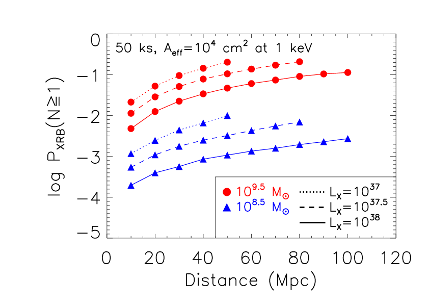
Whereas this study adopted a sensitivity threshold greater than erg s-1 to limit XRB contamination, similar snapshot exposures with the HDXI would achieve a sensitivity of erg s-1. This will lead to far more nuclear “sources” that are the sum of unresolved, lower luminosity XRBs, so we performed Lynx and AXIS simulations to determine the impact, and how depends on distance , resolution , exposure time , and other factors.
We simulated galaxies with in bins of 0.5 dex, with 10,000 galaxies per bin. We assumed that each galaxy is described by an exponential disk with a core radius kpc that is independent of mass. We used the methods from Section IV to populate each galaxy with XRBs, which involves drawing a number of XRBs per galaxy and assigning positions and luminosities for each one. LMXB positions were randomly distributed weighted by the surface brightness, whereas HMXBs were randomly distributed within a 1 kpc radius for SFR ranging from to 1 yr-1 (i.e., star formation outside of 1 kpc of the nucleus was ignored as these HMXBs will not be a problem). The XRBs were randomly assigned luminosities weighted by the XLF.
We simulated HDXI and AXIS observations using the simx software55 5 https://hea-www.harvard.edu/simx/, with the 2018 HDXI66 6 http://hea-www.cfa.harvard.edu/ jzuhone/soxs/responses.html and AXIS77 7 http://axis.astro.umd.edu/ responses. We assumed an absorbed power law spectrum for each XRB, with and cm-2 (Galactic absorption). We then projected the galaxies to and selected and , assuming a circular Gaussian PSF where is the on-axis half-power diameter. The PSF distortion with off-axis angle can be described by a second Gaussian term. We consider the effect of PSF blurring below.
Sources are detected using wavdetect, and for each XRB we compute the centroid error circle , where is the number of counts. We assume an optical galaxy centroid error of arcsec, and reject any detected, non-nuclear XRBs. The accuracy of the centroid positions are insensitive to . However, there is frequently a “glow” of X-rays from unresolved XRBs around the nucleus and from the wings of resolved XRBs. This glow is not uniformly distributed, but can be consistent with a weak nuclear point source and certainly impacts the centroid error circle. The proportion of galaxies with at least 5 counts within the nuclear aperture (using the 95% encircled energy radius) from this glow is approximately linear in . We compute by including the glow in the measured centroid error circle and counting galaxies as contaminated where there are at least 5 counts in the nuclear aperture from the glow.
Figure 6 shows the dependence of on for the cases of and , which represent the mass range of interest. This example uses an exposure time of 50 ks and the Lynx spectral response (effective area as a function of energy), scaled to a collecting area of 1 m2 at 1 keV. We computed over the range of parameters (assuming that SFR is proportional to mass, but not distributed in the same way) and find
| (8) |
where for the XLFs that we used. The dependence on comes from resolving and rejecting more of the glow, while the dependence on is from the nuclear aperture covering a larger physical area in the galaxy. If , then .
VI.4 Sensitivity and Number of Galaxies
We may now determine the best at each to optimize . Figure 7 shows as a function of and . Specifically, is defined in Figure 7 based on achieving 5% precision on , for a 68.3% confidence interval. At a given , must exceed 0.3 in order to keep below 1,000. This approach can be generalized to measuring in bins of 0.5 dex wide or to a continuous function (Miller et al. 2015). We use the former case to sketch the sensitivity requirements.

In a given mass bin, both and increase with sensitivity. The increase is linear for but not for ; for , , or well within the core of the distribution. Figure 3 shows that Chandra achieved this for a sensitivity of erg s-1 at . A reasonable approximation to the optimal sensitivity is ( if ). This approximation is based on the fact that decreases sharply as the sensitivity probes the core of the Gaussian distribution, but produce diminishing returns beyond. Meanwhile, is also a function of mass, so the applies at each mass bin.
For three mass bins , , and , the AMUSE-Field relation predicts optimal sensitivities of , 3, and erg s-1, respectively. At , using the prior analysis (Figure 6). These considerations lead to a conservative estimate of in each bin, or about 3000 galaxies overall at the low-mass end.
We can infer the existence of sufficient targets within 100 Mpc, where short HDXI snapshots are sufficient. Dobrycheva 2013 argue that there are about 37,000 galaxies in the SDSS in this volume, which covers 35% of the sky. The luminosity function for a flux-limited sample, with , implies that only about 10% of the detected galaxies are at (Schechter 1976; Binggeli et al. 1988). However, intrinsically there are more of these galaxies than the more massive ones, and the 10,000 detected in the SDSS in this range imply up to a factor of 3–10 more, depending on the slope of the luminosity function at (Blanton et al. 2005; Liu et al. 2008, ;).
Many of these will be LSBGs by definition, considering the SDSS sensitivity, which only make up 1.6% of the SDSS spectroscopic sample (Galaz et al. 2011). In the next decade, the Vera Rubin Observatory (Abell et al. 2009, VRO;) will survey more than 20,000 square degrees down to mag, so we expect at least 10,000 galaxies per mass bin. Although many will be unsuitable for observations (due to obscuration by the Galactic plane, proximity to bright sources, or morphology), there will easily be 1,000 candidate targets per bin. One challenge is that the photometric redshifts may not cleanly identify LSBGs within 100 Mpc (Greco et al. 2018), so some spectroscopic follow-up will be necessary.
VI.5 Strategy
Observing 3,000 galaxies through pointed observations would require 100 Ms of HDXI time, or three years. Here we investigate the potential for serendipitous sources to reduce the dedicated observing burden to measure . For the sake of argument, we assume two years of HDXI observations in a five-year mission with 75% observing efficiency (with the rest of the time allocated to the Lynx grating and microcalorimeter instruments). This amounts to 47 Ms. We further assume that the HDXI time is divided among long (150 ks), medium (50 ks), and short (10 ks) exposures with no field overlap, with allocations of 20%, 40%, and 40%, respectively.
This would cover 10.5 deg2, 63 deg2, and 315 deg2 for the long, medium, and short exposures. The sensitivities lead to distance limits, and thus to limiting volumes. At , the limiting distances are 25 Mpc, 50 Mpc, and 100 Mpc for the short, medium, and long exposures. For they are 40 Mpc, 90 Mpc, and 100 Mpc, and for they are all 100 Mpc. Assuming that the fields are observed at random, a few hundred galaxies could be observed in the two higher-mass bins but only a few tens of galaxies in the low-mass bin. This is the most conservative estimate because it wrongly assumes a uniform distribution, whereas a Chandra-like observing plan will target denser regions.
Cluster Outskirts
Galaxy clusters contain hundreds to thousands of galaxies and are of particular interest for X-ray observations. The cores of nearby clusters (Virgo, Fornax, Coma, and Perseus) have been well observed with Chandra, largely to study the intracluster medium (ICM). Future observations of the Perseus or Coma cores will be less useful for measuring because the ICM is so bright that reasonable exposures at HPD arcsec will not be sensitive enough for galaxies with . In addition, is lower in the Virgo core than in the field (Miller et al. 2012), which we expect to be an even stronger effect in the larger Perseus and Coma clusters. However, cluster outskirts remain under-studied and are a key area of interest for Lynx and AXIS. AXIS is particularly interesting because of its planned low-Earth orbit (Mushotzky 2018), which reduces the particle background and enables a cleaner study of accreting ICM at the outskirts. Tiled observations at the outskirts would likely capture a few thousand galaxies where the ICM surface brightness is low. These would be sensitive probes of at . LSBGs are an important part of this sample, as they make up a disproportionately large fraction of galaxies in clusters (likely due to ram-pressure stripping of gas).
Deep Fields
Miller et al. 2015 considered the role of deep fields; the 4 Ms Chandra Deep Field-South probes AGNs in sub- galaxies in a cosmological volume, so assuming a uniform Eddington ratio distribution (Aird et al. 2012), they showed that the distribution of X-ray detections probes . However, this is most effective above . Lynx and AXIS would create fields of equivalent depth in exposures of a few hundred ks, which would result in tens of such fields in the first few years of either mission. The main benefit to measuring at from the more distant objects is that the slope and scatter in the relation would be very tightly constrained, and possibly as a function of galaxy type or cosmological distance.
Normal Galaxies
Massive galaxies () are frequently targets of X-ray observations to study their hot gas, compact objects, or transient phenomena such as supernovae. However, dwarfs are clustered around more massive galaxies in the field (Binggeli et al. 1990), and based on their relative frequency we would expect each HDXI or AXIS field with a massive galaxy to have a number of dwarfs. Often, these will be unsuitable targets due to morphology or background, but especially within 100 Mpc galaxy observations will be important for building up a sample of targets. Chandra has observed numerous galaxies within this horizon, and we speculate that HDXI observations of these same galaxies would include at least 4,000 lower mass galaxies in fields with suitable sensitivity.
It is worth noting that these observations would also allow the detection of X-rays from MBHs in stripped dwarf nuclei (frequently former nuclear star clusters), such as in the ultra-compact dwarf M60-UCD1 (Strader et al. 2013; Seth et al. 2014). A significant fraction of local MBHs (up to 1/3) may be located in such systems (Voggel et al. 2019), and for relatively nearby galaxies they can be easily identified via VRO and Wide-Field Infrared Space Telescopes (WFIRST) colors (Muñoz et al. 2014, using methods developed by). We expect several around each galaxy relevant for the measurement (Kruijssen et al. 2019, for the Milky Way, about 6 have been found;), so a serendipitous sample of 1000 is easily feasible during the HDXI lifetime.
Targeted Survey
There will almost certainly be enough serendipitous sources at to constrain to 5% precision, and so a major component of the program is “free,” requiring only that one waits several years. However, at the lowest masses it is much less certain that enough galaxies will be observed because the sensitivity of the typical field only captures systems within Mpc. There will not likely be enough deeper observations to make up for this limit by measuring at a lower sensitivity.
This motivates a snapshot survey of very nearby dwarf galaxies, many of which will be LSBGs. We estimate that 200-400 targets are required, with exposure times between 5-15 ks. This leads to a maximum total exposure time of 3 Ms. A dedicated survey of the Virgo cluster would significantly reduce the total time, since many of the nearby dwarf galaxies will be found in and around the cluster. If fields are selected to contain an average of two good candidates, the total observing burden is reduced to 1.5 Ms, which is a large program but a modest investment for measuring .
VII Summary
We searched for nuclear X-ray sources in 32 nearby LSBGs with Chandra and found 3-4, which we judge as very likely to be MBHs. This leads to , which is consistent with the expectation from the best-fitting correlation from the AMUSE-Field study (Miller et al. 2012), which used Chandra images of high surface brightness, early-type galaxies with almost no gas. However, is inconsistent with the same relation if is replaced by the total baryonic mass, which is important since LSBGs have large gas fractions.
This result suggests that weak nuclear activity innearby LSBGs with regular morphology is similar to that in normal galaxies of the same stellar mass, and thus that MBH growth is somehow tied to stellar, rather than baryonic or dynamical, mass. One explanation could be that isolated LSBGs are inefficient at concentrating gas that would lead both to star formation and MBH growth. However, the sample size is too small to independently measure any relationship between and (or total baryonic mass) in LSBGs, and a deeper, more extensive X-ray survey is needed to do this. Such a survey would also be able to answer whether the nuclear activity is better correlated with bulge luminosity, as argued by Galaz et al. 2011 for LSBGs, or total stellar mass. Nevertheless, our result supports a scenario in which MBHs co-evolve with the stellar component, rather than forming prior to it or in a way that correlates with halo mass.
The agreement with the AMUSE-Field correlation also suggests that LSBGs can be used to constrain the local of MBHs, albeit with too few detected sources to independently measure an relationship. LSBGs provide many relatively isolated targets with , where predictions differ between heavy- and light-seed theories of MBH formation. A dedicated program, spaced over about five years, with a new, high resolution, wide-field X-ray camera such as Lynx or AXIS would enable a measurement of to a precision of several percent, thereby providing a strong local boundary condition on all MBH formation and evolution models, and extending studies of black-hole feedback to the low-mass end of the luminosity function.
References
- Abell et al. (2009) Abell, P. A., Allison, J., Anderson, S. F., et al. 2009. https://arxiv.org/abs/0912.0201
- Aird et al. (2012) Aird, J., Coil, A. L., Moustakas, J., et al. 2012, ApJ, 746, 90, doi: 10.1088/0004-637X/746/1/90
- Alam et al. (2015) Alam, S., Albareti, F. D., Allende Prieto, C., et al. 2015, ApJS, 219, 12, doi: 10.1088/0067-0049/219/1/12
- Asmus et al. (2011) Asmus, D., Gandhi, P., Smette, A., Hönig, S. F., & Duschl, W. J. 2011, A&A, 536, A36, doi: 10.1051/0004-6361/201116693
- Ayres (2004) Ayres, T. R. 2004, ApJ, 608, 957, doi: 10.1086/420688
- Bell et al. (2003) Bell, E. F., McIntosh, D. H., Katz, N., & Weinberg, M. D. 2003, ApJS, 149, 289, doi: 10.1086/378847
- Binggeli et al. (1988) Binggeli, B., Sandage, A., & Tammann, G. A. 1988, ARA&A, 26, 509, doi: 10.1146/annurev.aa.26.090188.002453
- Binggeli et al. (1990) Binggeli, B., Tarenghi, M., & Sandage, A. 1990, A&A, 228, 42
- Blanton et al. (2005) Blanton, M. R., Lupton, R. H., Schlegel, D. J., et al. 2005, ApJ, 631, 208, doi: 10.1086/431416
- Blanton & Moustakas (2009) Blanton, M. R., & Moustakas, J. 2009, ARA&A, 47, 159, doi: 10.1146/annurev-astro-082708-101734
- Bothun et al. (1997) Bothun, G., Impey, C., & McGaugh, S. 1997, PASP, 109, 745, doi: 10.1086/133941
- Bothun et al. (1987) Bothun, G. D., Impey, C. D., Malin, D. F., & Mould, J. R. 1987, AJ, 94, 23, doi: 10.1086/114443
- Chambers et al. (2016) Chambers, K. C., Magnier, E. A., Metcalfe, N., et al. 2016, arXiv e-prints, arXiv:1612.05560. https://arxiv.org/abs/1612.05560
- Courtois et al. (2009) Courtois, H. M., Tully, R. B., Fisher, J. R., et al. 2009, AJ, 138, 1938, doi: 10.1088/0004-6256/138/6/1938
- Dalcanton et al. (1997) Dalcanton, J. J., Spergel, D. N., Gunn, J. E., Schmidt, M., & Schneider, D. P. 1997, AJ, 114, 635, doi: 10.1086/118499
- Das et al. (2009) Das, M., Reynolds, C. S., Vogel, S. N., McGaugh, S. S., & Kantharia, N. G. 2009, ApJ, 693, 1300, doi: 10.1088/0004-637X/693/2/1300
- Dobrycheva (2013) Dobrycheva, D. V. 2013, Odessa Astronomical Publications, 26, 187
- Douna et al. (2015) Douna, V. M., Pellizza, L. J., Mirabel, I. F., & Pedrosa, S. E. 2015, A&A, 579, A44, doi: 10.1051/0004-6361/201525617
- Foord et al. (2017) Foord, A., Gallo, E., Hodges-Kluck, E., et al. 2017, ApJ, 841, 51, doi: 10.3847/1538-4357/aa6d63
- Freeman et al. (2002) Freeman, P. E., Kashyap, V., Rosner, R., & Lamb, D. Q. 2002, ApJS, 138, 185, doi: 10.1086/324017
- Galaz et al. (2011) Galaz, G., Herrera-Camus, R., Garcia-Lambas, D., & Padilla, N. 2011, ApJ, 728, 74, doi: 10.1088/0004-637X/728/2/74
- Gallo et al. (2008) Gallo, E., Treu, T., Jacob, J., et al. 2008, ApJ, 680, 154, doi: 10.1086/588012
- Gallo et al. (2019) Gallo, E., Hodges-Kluck, E., Treu, T., et al. 2019, arXiv e-prints. https://arxiv.org/abs/1903.06629
- Gaskin et al. (2018) Gaskin, J. A., Dominguez, A., Gelmis, K., et al. 2018, in Society of Photo-Optical Instrumentation Engineers (SPIE) Conference Series, Vol. 10699, 106990N, doi: 10.1117/12.2314149
- Gehrels (1986) Gehrels, N. 1986, ApJ, 303, 336, doi: 10.1086/164079
- Gilfanov (2004) Gilfanov, M. 2004, MNRAS, 349, 146, doi: 10.1111/j.1365-2966.2004.07473.x
- Graham (2003) Graham, A. W. 2003, AJ, 125, 3398, doi: 10.1086/375000
- Greco et al. (2018) Greco, J. P., Greene, J. E., Strauss, M. A., et al. 2018, ApJ, 857, 104, doi: 10.3847/1538-4357/aab842
- Gültekin et al. (2009) Gültekin, K., Richstone, D. O., Gebhardt, K., et al. 2009, ApJ, 698, 198, doi: 10.1088/0004-637X/698/1/198
- Haberzettl et al. (2007) Haberzettl, L., Bomans, D. J., & Dettmar, R.-J. 2007, A&A, 471, 787, doi: 10.1051/0004-6361:20066918
- Huchtmeier & Richter (1989) Huchtmeier, W. K., & Richter, O.-G. 1989, A General Catalog of HI Observations of Galaxies. The Reference Catalog., 350
- Impey & Bothun (1997) Impey, C., & Bothun, G. 1997, ARA&A, 35, 267, doi: 10.1146/annurev.astro.35.1.267
- Impey et al. (2001) Impey, C., Burkholder, V., & Sprayberry, D. 2001, AJ, 122, 2341, doi: 10.1086/323537
- Kalberla et al. (2005) Kalberla, P. M. W., Burton, W. B., Hartmann, D., et al. 2005, A&A, 440, 775, doi: 10.1051/0004-6361:20041864
- Kennicutt (1998) Kennicutt, Jr., R. C. 1998, ApJ, 498, 541, doi: 10.1086/305588
- Kewley et al. (2006) Kewley, L. J., Groves, B., Kauffmann, G., & Heckman, T. 2006, MNRAS, 372, 961, doi: 10.1111/j.1365-2966.2006.10859.x
- Kim et al. (2013) Kim, D. W., Fabbiano, G., Ivanova, N., et al. 2013, ApJ, 764, 98, doi: 10.1088/0004-637X/764/1/98
- Kormendy & Ho (2013) Kormendy, J., & Ho, L. C. 2013, ARA&A, 51, 511, doi: 10.1146/annurev-astro-082708-101811
- Kruijssen et al. (2019) Kruijssen, J. M. D., Pfeffer, J. L., Reina-Campos, M., Crain, R. A., & Bastian, N. 2019, MNRAS, 486, 3180, doi: 10.1093/mnras/sty1609
- Lee et al. (2019) Lee, N., Gallo, E., Hodges-Kluck, E., et al. 2019, arXiv e-prints. https://arxiv.org/abs/1902.03328
- Lehmer et al. (2010) Lehmer, B. D., Alexander, D. M., Bauer, F. E., et al. 2010, ApJ, 724, 559, doi: 10.1088/0004-637X/724/1/559
- Lehmer et al. (2016) Lehmer, B. D., Basu-Zych, A. R., Mineo, S., et al. 2016, ApJ, 825, 7, doi: 10.3847/0004-637X/825/1/7
- Lehmer et al. (2019) Lehmer, B. D., Eufrasio, R. T., Tzanavaris, P., et al. 2019, ApJS, 243, 3, doi: 10.3847/1538-4365/ab22a8
- Liu et al. (2008) Liu, C. T., Capak, P., Mobasher, B., et al. 2008, ApJ, 672, 198, doi: 10.1086/522361
- Makarov et al. (2014) Makarov, D., Prugniel, P., Terekhova, N., Courtois, H., & Vauglin, I. 2014, A&A, 570, A13, doi: 10.1051/0004-6361/201423496
- McGaugh (1996) McGaugh, S. S. 1996, MNRAS, 280, 337, doi: 10.1093/mnras/280.2.337
- Mei et al. (2009) Mei, L., Yuan, W.-M., & Dong, X.-B. 2009, Research in Astronomy and Astrophysics, 9, 269, doi: 10.1088/1674-4527/9/3/002
- Merloni et al. (2003) Merloni, A., Heinz, S., & di Matteo, T. 2003, MNRAS, 345, 1057, doi: 10.1046/j.1365-2966.2003.07017.x
- Miller et al. (2012) Miller, B., Gallo, E., Treu, T., & Woo, J.-H. 2012, ApJ, 747, 57, doi: 10.1088/0004-637X/747/1/57
- Miller et al. (2015) Miller, B. P., Gallo, E., Greene, J. E., et al. 2015, ApJ, 799, 98, doi: 10.1088/0004-637X/799/1/98
- Minchin et al. (2004) Minchin, R. F., Disney, M. J., Parker, Q. A., et al. 2004, MNRAS, 355, 1303, doi: 10.1111/j.1365-2966.2004.08409.x
- Mineo et al. (2012) Mineo, S., Gilfanov, M., & Sunyaev, R. 2012, MNRAS, 419, 2095, doi: 10.1111/j.1365-2966.2011.19862.x
- Monet et al. (2003) Monet, D. G., Levine, S. E., Canzian, B., et al. 2003, AJ, 125, 984, doi: 10.1086/345888
- Morrissey et al. (2005) Morrissey, P., Schiminovich, D., Barlow, T. A., et al. 2005, ApJ, 619, L7, doi: 10.1086/424734
- Muñoz et al. (2014) Muñoz, R. P., Puzia, T. H., Lançon, A., et al. 2014, ApJS, 210, 4, doi: 10.1088/0067-0049/210/1/4
- Mushotzky (2018) Mushotzky, R. 2018, ArXiv e-prints. https://arxiv.org/abs/1807.02122
- Nguyen et al. (2018) Nguyen, D. D., Seth, A. C., Neumayer, N., et al. 2018, ApJ, 858, 118, doi: 10.3847/1538-4357/aabe28
- Nguyen et al. (2019) Nguyen, D. D., den Brok, M., Seth, A. C., et al. 2019, arXiv e-prints, arXiv:1902.03813. https://arxiv.org/abs/1902.03813
- Peacock & Zepf (2016) Peacock, M. B., & Zepf, S. E. 2016, ApJ, 818, 33, doi: 10.3847/0004-637X/818/1/33
- Ramya et al. (2011) Ramya, S., Prabhu, T. P., & Das, M. 2011, MNRAS, 418, 789, doi: 10.1111/j.1365-2966.2011.19530.x
- Rosenbaum et al. (2009) Rosenbaum, S. D., Krusch, E., Bomans, D. J., & Dettmar, R. J. 2009, A&A, 504, 807, doi: 10.1051/0004-6361/20077462
- Sazonov & Khabibullin (2017) Sazonov, S., & Khabibullin, I. 2017, MNRAS, 468, 2249, doi: 10.1093/mnras/stx626
- Schechter (1976) Schechter, P. 1976, ApJ, 203, 297, doi: 10.1086/154079
- Schombert (1998) Schombert, J. 1998, AJ, 116, 1650, doi: 10.1086/300558
- Schombert et al. (1992) Schombert, J. M., Bothun, G. D., Schneider, S. E., & McGaugh, S. S. 1992, AJ, 103, 1107, doi: 10.1086/116129
- Schombert et al. (2001) Schombert, J. M., McGaugh, S. S., & Eder, J. A. 2001, AJ, 121, 2420, doi: 10.1086/320398
- Secrest et al. (2015) Secrest, N. J., Dudik, R. P., Dorland, B. N., et al. 2015, ApJS, 221, 12, doi: 10.1088/0067-0049/221/1/12
- Seth et al. (2008) Seth, A., Agüeros, M., Lee, D., & Basu-Zych, A. 2008, ApJ, 678, 116, doi: 10.1086/528955
- Seth et al. (2014) Seth, A. C., van den Bosch, R., Mieske, S., et al. 2014, Nature, 513, 398, doi: 10.1038/nature13762
- She et al. (2017) She, R., Ho, L. C., & Feng, H. 2017, ApJ, 842, 131, doi: 10.3847/1538-4357/aa7634
- Sprayberry et al. (1995) Sprayberry, D., Impey, C. D., Bothun, G. D., & Irwin, M. J. 1995, AJ, 109, 558, doi: 10.1086/117300
- Strader et al. (2013) Strader, J., Seth, A. C., Forbes, D. A., et al. 2013, ApJ, 775, L6, doi: 10.1088/2041-8205/775/1/L6
- Subramanian et al. (2016) Subramanian, S., Ramya, S., Das, M., et al. 2016, MNRAS, 455, 3148, doi: 10.1093/mnras/stv2500
- Trump et al. (2015) Trump, J. R., Sun, M., Zeimann, G. R., et al. 2015, ApJ, 811, 26, doi: 10.1088/0004-637X/811/1/26
- van den Bosch et al. (2015) van den Bosch, R. C. E., Gebhardt, K., Gültekin, K., Yıldırım, A., & Walsh, J. L. 2015, ApJS, 218, 10, doi: 10.1088/0067-0049/218/1/10
- Voggel et al. (2019) Voggel, K. T., Seth, A. C., Baumgardt, H., et al. 2019, ApJ, 871, 159, doi: 10.3847/1538-4357/aaf735
- Vollmer et al. (2013) Vollmer, B., Perret, B., Petremand, M., et al. 2013, AJ, 145, 36, doi: 10.1088/0004-6256/145/2/36
- Volonteri (2012) Volonteri, M. 2012, Science, 337, 544, doi: 10.1126/science.1220843