Determination of the escape velocity of the Milky Way using a proper motion selected halo sample
Abstract
Context. The Gaia mission has provided the largest catalogue ever of sources with tangential velocity information. However, using this catalogue for dynamical studies is difficult because most of the stars lack line-of-sight velocity measurements. Recently, we presented a selection of halo stars with accurate distances that have been selected based on their photometry and proper motions.
Aims. Using this sample, we model the tail of the velocity distribution in the stellar halo, locally and as a function of distance. Our goal is to measure the escape velocity, and herewith to constrain the mass of our Galaxy.
Methods. We fit the tail of the velocity distribution with a power-law distribution, a commonly used approach first established by Leonard & Tremaine 1990. For the first time ever we use tangential velocities measured accurately for an unprecedented number of halo stars to estimate the escape velocity.
Results. In the solar neighbourhood, we obtain a very precise estimate of the escape velocity which is . This estimate is most likely biased low, our best guess is by 10%. As a result, the true escape velocity most likely is closer to . The escape velocity directly constrains the total mass of the Milky Way. To find the best fitting halo mass and concentration parameter we adjusted the dark (spherical NFW) halo of a realistic Milky Way potential while keeping the circular velocity at the solar radius fixed at . The resulting halo parameters are and concentration parameter , where we use the explicit notation to indicate that these have been corrected for the 10% bias. The slope of the escape velocity with galactocentric distance is as expected in the inner Galaxy based on Milky Way models. Curiously, we find a disagreement beyond the solar radius where the estimated escape velocity is larger than at the solar radius. This result is likely an effect of a change in the shape of the velocity distribution and could be related to the presence of velocity clumps. A tentative analysis of the escape velocity as a function of shows that the slope is shallower than expected for a spherical halo using standard values for the characteristic parameters describing the galactic disc.
Key Words.
Galaxy: kinematics and dynamics – Galaxy: structure – Galaxy: fundamental parameters1 Introduction
Numerous studies have attempted to measure the mass of the Milky Way, yet it has been notoriously difficult to obtain precise and model independent constraints. Most works now agree that the mass of the Milky Way’s dark matter halo is within a factor of two (see Fig. 7 of Callingham et al. 2019, for a recent compilation). The kinematics of globular clusters, dwarf galaxies, and halo stars have often been used in such studies (Kochanek 1996; Xue et al. 2008; Watkins et al. 2010; Deason et al. 2012; Fragione & Loeb 2017; Posti & Helmi 2019; Callingham et al. 2019; Fritz et al. 2020). The timing argument and the properties of debris streams such as those from the Sagittarius dwarf (Dierickx & Loeb 2017; Zaritsky et al. 2020, e.g.) have provided additional, yet similar constraints. In this work, we aim to derive a very precise estimate of the escape velocity near the Sun and hence, under further assumptions, of the mass of the Milky Way.
The escape velocity is the maximum velocity that stars can have while still being bound to the Galaxy. In principle, the single fastest moving bound star places a lower limit on the escape velocity. However, in practice, individual stars might be affected by large measurement uncertainties or they might be outliers (such as escapees). A more robust approach is to fit the velocity distribution as a whole as put forward by Leonard & Tremaine 1990, who describe the tail of the velocity distribution with a power-law.
Several works have used the LT90 method in the past. For example, Smith et al. 2007 and Piffl et al. 2014b, hereafter S07 and P14, estimated the escape velocity locally to lie in the range of km/s, using only radial velocity information from RAVE (Steinmetz et al. 2006). The analysis of Williams et al. 2017 supports these values and these authors also show that the escape velocity drops to km/s at a distance of 50 kpc. The advent of full phase-space information with Gaia DR2 has not led to a reduction in the estimated range for the escape velocity in the solar neighbourhood: it is still km/s (Monari et al. 2018; Deason et al. 2019, hereafter M18 and D19), a result that can largely be attributed to the different underlying assumptions used by the authors.
In this paper, we will use a sample of halo stars with only tangential velocities from Gaia DR2 to infer the escape velocity applying also the LT90 method. This sample comprises orders of magnitude more halo stars than any other sample used before. Samples making use of only tangential velocities have not been popular for this kind of studies in the past because of the large uncertainties in the velocities, particularly induced by the distance uncertainties. Even more dramatic was the lack of (accurate) proper motion measurements for large numbers of stars. However, Gaia DR2, containing about more stars with proper motions than radial velocities, makes this kind of study feasible now. We proceed in this work as follows. We describe the data used and its properties in Sec. 2 and the methods used in Sec. 3. In Sec. 4 we test the method for determining the escape velocity using mock data and cosmological simulations. In Sec. 5 and Sec. 6 we present our results in the solar neighbourhood and as a function of galactocentric distance, respectively. In Sec. 7 we use the local escape velocity to derive an estimate of the mass of the Milky Way’s dark halo and to identify likely unbound stars. In Sec. 8 we present our conclusions.
2 Data
The determination of the escape velocity is contingent upon having a sample of halo stars with high-quality measurements and large velocity amplitudes. Most of the data used in this work is provided by the Gaia mission (Gaia Collaboration et al. 2016; Gaia Collaboration, Brown et al. 2018). We will mainly use the sample of halo stars selected and analysed in Koppelman & Helmi 2021. This sample comprises Main Sequence (MS) halo stars and we refer to it as the reduced proper motion or the 5D sample hereafter. Additionally, we will also make use of a set of nearby halo stars with full phase-space information.
2.1 Velocity information
To transform the observed motions (proper motions and radial velocities when available) into space velocities we proceed as follows. We compute the tangential velocity of a star by combining the proper motion and its distance as
| (1) |
where . These velocities are then corrected for the solar motion using the values for the motion of the Sun with respect to the local standard of rest (LSR) given by Schönrich et al. 2010 and the motion of the LSR given by McMillan 2017; they are and respectively. The transformations to correct the tangential velocities are
| (2) |
where and are defined as
| (3a) | |||
| (3b) |
Finally, the tangential velocity in the Galactic frame of rest as observed from the Sun is calculated as
| (4) |
Similarly the line-of-sight velocity can be corrected for the solar reflex motion using , where
| (5) |
To derive space velocities we use the following expressions:
| (6a) | |||
| (6b) | |||
| (6c) |
To transform the coordinates to a galactocentric frame we place the Sun at kpc (McMillan 2017). We use this value for the distance to the Galactic centre because it is consistent with the McMillan 2017 potential that we will employ later, and the same is true for the LSR velocity. We note however that the McMillan 2017 values agree well with the more recent determination of the distance to the Galactic Centre by the GRAVITY Collaboration et al. 2018 and circular velocity at the position of the Sun by Eilers et al. 2019.
To isolate a halo sample using the Gaia DR2 data, we consider stars with velocity vectors that deviate more than km/s from the velocity vector of the LSR (i.e. the velocity vector of a typical disc star), namely . This type of selection is known as a ‘Toomre’ selection.
When no line-of-sight velocity information is available, we use Eq. (6) setting to zero. In that case, we refer to the velocity vector as to stress that these are not the true Cartesian velocities. For this set of stars, which constitute the majority of our sample, we use an adapted Toomre selection to isolate a halo sample, namely .
2.2 Sample with full phase-space information
In the solar neighbourhood, we will use a sample of stars with full phase-space information from Gaia known as the 6D or the radial velocity spectrometer (RVS) sample (Katz et al. 2019). We extend this dataset by adding sources with radial velocities observed by APOGEE (Wilson et al. 2010; Abolfathi et al. 2018), LAMOST (Cui et al. 2012), and RAVE (Kunder et al. 2017), see Sec. 2 of Koppelman et al. 2019 for a full description of this catalogue. The cross-matches with APOGEE and RAVE have been obtained from the Gaia archive (Marrese et al. 2019).
For this sample and in line with M18 and D19, we use the quality cuts described in Marchetti et al. 2019, namely
- •
,
- •
,
- •
,
- •
,
- •
,
and also impose the following quality criteria:
- •
,
- •
.
For the additional spectroscopic data we use the same quality cuts, with exception of the criterion on rv_nb_transits. Additionally, we use survey-specific quality constraints. For APOGEE we use
- •
,
- •
,
- •
,
- •
,
for RAVE
- •
,
- •
,
- •
,
and for LAMOST
- •
,
- •
.
Several studies have reported that the sources in the RVS sample, and bright sources in general, contain a parallax offset of mas (Schönrich et al. 2019; Leung & Bovy 2019; Zinn et al. 2019; Chan & Bovy 2020, see). Therefore, we correct the parallaxes in the 6D sample for an offset of mas as estimated by Schönrich et al. 2019. Following these authors, we increase the parallax uncertainties by mas to account for the uncertainties in the offset and by mas to account for the RMS in the offset reported by Lindegren et al. 2018, both of which are added in quadrature.
Nonetheless, to mitigate the effects of the parallax offset we only consider sources within 2 kpc. As explained earlier we select halo stars as those with . Finally, we remove the star with Gaia DR2 source_id 5932173855446728064 since its radial velocity reported in Gaia DR2 is known to be incorrect (Boubert et al. 2019). The final sample comprises 2067 high-quality stars, of which 495 are from the Gaia RVS sample, 10 from APOGEE, one from RAVE, and 1561 from LAMOST.
Since the spectroscopic surveys add a considerable number of stars, mostly from LAMOST, we have checked that they do not bias our results. In fact, these are fully consistent with using only Gaia RVS sources. The stars from the spectroscopic surveys do not dominate the determination of because they, in general, have larger uncertainties. However, they do help in closing the confidence contours, as we will see in Sec. 5.
2.3 The reduced proper motion sample
For the complete description of the reduced proper motion (RPM) sample we refer the reader to the KH21 paper. Here we will summarise the details that are relevant for this paper. By virtue of the selection method, the RPM sample comprises only MS stars. The relatively linear colour - magnitude relation for these types of stars can be used to calculate photometric distances with typical uncertainties of .
In KH21 we have already introduced several quality cuts, here we prune the sample even further. In summary, we:
- 1.
Target the most pure set of halo stars: (see Sec. 2.1).
- 2.
Select stars with large tangential velocities: km/s.
- 3.
Isolate stars that are the least affected by extinction, that is we consider only those with .
- 4.
Select stars in the colour range where the photometric distances have the smallest uncertainty: . The blue limit here is stricter than in KH21, to remove any possible contamination from the MS turn-off.
- 5.
Select stars at high latitudes to remove contamination from the disc: .
Some stars in the RPM sample have less precise photometric distance than trigonometric distance (i.e. parallax from Gaia). Furthermore, some stars may have been excluded because they did not satisfy the last three quality cuts described above, even though their trigonometric parallaxes are accurate. Therefore we add such stars back to the sample. We also replace the photometric distances with trigonometric distances for stars with , if the latter has a smaller uncertainty than the first, and we only consider stars with parallaxes .
As mentioned above, the trigonometric parallaxes from Gaia DR2 are known to contain a zero-point offset that has a complex dependence on other observational parameters (e.g. the colour and magnitude of the stars). Because most of the stars in the 5D sample (without radial velocities) are fainter than those in the 6D sample, we correct their parallaxes with a different offset. Following Lindegren et al. 2018, we use a value of mas for the parallax offset and increase the parallax uncertainties by mas (the uncertainties are added in quadrature) to account for variations in the offset.
Within 1 kpc about of the distances stem from the Gaia parallaxes and at 2 kpc this percentage drops to . The final, pruned sample comprises sources of which have Gaia parallaxes.
2.4 Inspection of the RPM sample
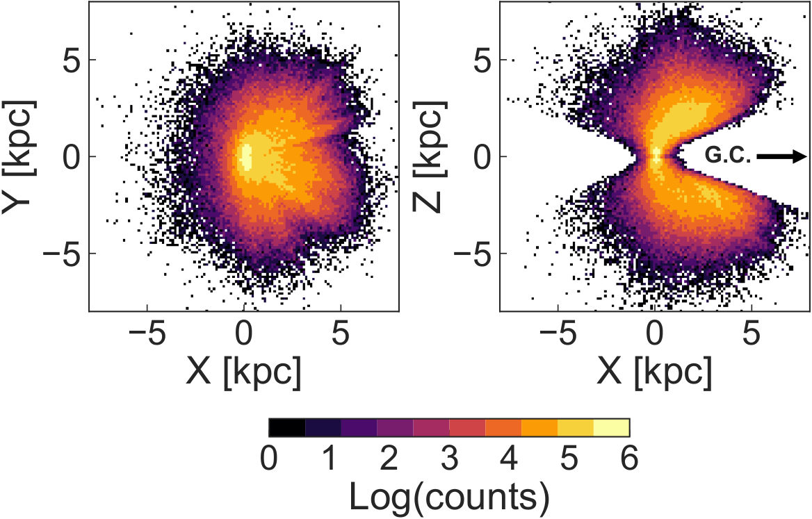
Figure 1 shows the spatial distribution of the stars in the sample. The maps are coloured by the logarithm of the counts per bin. The quality cuts described in the previous section affect the spatial distribution of the stars, most notably by removing low-latitude stars. The overdensity at the solar neighbourhood (centre of the figure) is caused by the addition of sources with accurate parallaxes. The median heliocentric distance of the sample is kpc.
In Fig. 2 we show the tail of the tangential velocity distribution as a function of galactocentric distance by slicing the sample in uniformly spaced overlapping bins, ranging from kpc, of kpc width, which is larger than the typical uncertainty in the distances. A visual inspection reveals only small variations in the distributions. These clearly resemble a power-law (as anticipated) but with a slight tendency to become more exponential with distance from the Galactic Centre.
We propagated the uncertainties in the tangential velocities, which we denote as , using the standard uncertainty propagation approximation. This approximation uses a Taylor expansion to linearize the coordinate transformations, which is a common practice in the literature. We start the propagation from the measurement uncertainties of Gaia DR2, where the uncertainty of the distance is derived from the parallax uncertainty for the trigonometric sample. For the RPM sample, we derive distance uncertainties separately since this sample contains photometric distances (see Sec. 3.3. of KH21 for more information). Typically, the photometric distance uncertainties are at the level.
The distribution of the relative uncertainties in the tangential velocity is shown in Fig. 3, separately for the photometric (in blue) and trigonometric distances (in green). On average, the tangential velocities derived from the trigonometric parallaxes are slightly more accurate than those based on the photometric distances. This is a selection effect since only sources with very accurate parallaxes are included in our sample. When propagating the uncertainties in the velocities, we find that the uncertainty distribution for sources with photometric distances peaks at and has a median of . For the trigonometric distances, the distribution in the velocity uncertainties peaks at . The distribution of has a tail towards higher uncertainties because of proper motions uncertainties and there is only is a small dependence with magnitude at the faint end (i.e. for .
3 Methods
3.1 Determining
As described earlier, we will use here the LT90 method to determine the escape velocity, denoted hereafter as . The motivation of this method is that the tail of the velocity distribution can be described by a power-law, and is the velocity at which the probability of finding a star goes to zero. Although we follow closely Sections IIa and IIc from LT90 and adopt their notation, the formalism we use reveals some differences.
As just stated, the probability of finding a star in a local volume with a velocity in the range is described close to the escape velocity as a power-law
| (7) |
where is the exponent, is the escape velocity, and is a threshold velocity below which the distribution is not well-represented by a power-law. It is important to set accordingly such that only the tail of the distribution is fit. The normalisation constant is defined as , which is obtained from .
The expression in Eq. (7) describes the distribution of velocities corrected for the solar motion (including peculiar and LSR), for example at the location of the Sun. Note that if is the probability of finding a star with velocity in the range , this implies that there exists some distribution such that under the assumption that the velocity distribution is isotropic.
We now wish to obtain the probability distribution for the tangential velocity (i.e. ). This can be derived from the joint distribution which gives the probability of finding a star with a given line-of-sight velocity and tangential velocity as . By performing a transformation of variables
| (8) |
where is a unit vector along the line-of-sight. To express the distribution function in terms of only we integrate over the line-of-sight component (and over angle)
| (9) |
The distribution gives the probability of finding a tangential velocity in the range .
Evaluating this integral in spherical coordinates, with aligned with the -axis (implicitly assuming the stars are distributed isotropically), we obtain
| (10) |
which, by changing the order of integration and the substitution of , reduces to
| (11) |
The resulting integral for given by Eq. (7) can be solved with Mathematica (and depends on the regularised hypergeometric function). When evaluating the Taylor series expansion of for the integral, we obtain
| (12) |
which the expression found by LT90. It can be normalised by multiplying with the constant , which is derived from the requirement that , and where we have replaced with for clarity. The reason for this is that only in the case of are the two power-law indices of Eq. (7) and Eq. (12) related, and . It is thus best to think of in Eq. (12) simply as a power-law description of the tangential velocity tail, an approximation which is supported by Fig. 2. We will see in Sec. 4.1 that it is in general not quite true that for the values that are typically considered in the literature. In what follows, we thus reserve the notation for the power-law exponent of , use for the exponent using the distribution from Eq. (7) and use to indicate the exponent for a sample using only line-of-sight velocities (e.g. when comparing to values in the literature).
So far we have assumed that the velocities ( and ) are the true velocities. However, in reality we are dealing with ‘observed’ velocities, which are a combination of the true velocity and some unknown uncertainty. In this section we will use to indicate the observed tangential velocity and reserve for the true value. To account for the uncertainty we smooth the velocities by convolving them with an error distribution , where is the uncertainty in . If we assume that and have Gaussian errors, then the distribution follows the Beckmann distribution11 1 The Beckmann distribution is the most general form of the distribution of parameter , where and drawn from a bivariate Gaussian distribution (see https://reference.wolfram.com/language/ref/BeckmannDistribution.html). The distribution generally can only be expressed in integral form (e.g. Eq. 31 of Beckmann 1962) but takes an explicit form for specific cases. For example, when and are independent and drawn from a standard normal distribution, takes the form of the Rice distribution. The more general case of , with and are drawn from an uncorrelated bivariate Gaussian distribution, is known as the non-central chi distribution. (i.e. it is non-Gaussian). However, if evaluated far away from the origin , this distribution is well-approximated by a Gaussian. This gives us another reason to choose a sufficiently large . Therefore, in what follows we approximate by a Gaussian . The convolution of the power-law from Eq. (12) and the Gaussian is given by
| (13) |
where .
We note that we have taken as the integration lower boundary and not zero as in Eq. (17) of LT90. Since the velocity distribution below is not well-described by a power-law, but by a different distribution function , the convolution over the range , would take the form
| (14) |
which does not depend on nor on . As we will see below, we may thus ignore this part of the velocity distribution. This also means that we also ignore stars that have an apparent below the cut, but with a finite probability of having a true above it. We will see in Sec. 4 that these assumptions do not affect the method’s ability to infer .
By normalising Eq. (13) we find , the probability of finding a star with in the range (
| (15) |
By definition, because both and are normalised, the integral in the denominator is unity, as the area under a convolution is . The resulting likelihood function is given by
| (16) |
The probability distribution of the model parameters and is found by using Bayes’ theorem
| (17) |
where and are priors for and . For numerical reasons the logarithm of the probability is evaluated, which also allows us to ignore the normalisation since that is constant and independent of the model parameters.
The procedure that is outlined above implicitly makes the following assumptions:
- 1.
The tail of the velocity distribution is populated up to the escape velocity.
- 2.
The tail of the velocity distribution is smooth.
- 3.
There are no unbound stars in our sample.
- 4.
And there is no contamination from a rotating (disc-like) population, which would break the isotropy on the sky.
Perhaps the most problematic assumption is the first one. There is no guarantee that the velocity distribution locally, or at any other location in the Milky Way, extends up to the escape velocity. Most likely it is truncated at some lower value. As a result, the LT90 method is prone to underestimate the true . For example, cosmological simulations show velocity distributions that are truncated at of (e.g. S07). The exact location of the truncation depends on the assembly history of the galaxy and quite possibly also on the resolution of the simulation. We will quantify the truncation of the velocity distribution using mock data in Sec. 4. We stress that, because of this truncation, whatever value we derive for it most likely is a lower limit.
The second assumption has recently been tested by Grand et al. 2019, who find that clustering in the velocity distribution biases the estimation of , and can result both in under and overestimates. Nonetheless, these authors show that the estimated is typically underestimated by . To emphasise the importance of this bias: a difference of in the escape velocity results in a bias in the estimated mass.
It seems unlikely that our sample contains many unbound stars, since hyper-velocity stars are typically young stars ejected from the Galactic Centre and not old stars in the halo (Brown 2015; Boubert et al. 2018, e.g.). Furthermore, the velocity distributions shown in Fig. 2 are relatively smooth, suggesting the presence of a single population dominated by main sequence halo stars. Nonetheless, it would be interesting to follow-up spectroscopically stars near the escape velocity. In Sec. 7.3 we will revisit possible outliers in the solar neighbourhood.
3.2 Adopting a prior on and
In line with the literature, we assume a simple prior on of the form . For (we will use the notation here, understanding that it only compares to and in the limiting case) there is some debate in the literature on what to assume, and since and are highly degenerate (see next section), the prior assumed might bias the resulting . For example, the M18 and D19 estimates of differ by mainly because of the different ranges considered for . Attempting to estimate and simultaneously is only possible with a large sample with very small uncertainties. For example, LT90 estimated that a sample of stars with high-quality radial-velocities above is necessary to estimate both values simultaneously.
LT90 argue that -values should be in the range , because this brackets , which is the value expected for a system that has undergone violent relaxation (Aguilar & White 1986; Jaffe 1987; Tremaine 1987). S07 have compared stellar halos in cosmological simulations of Milky Way-like galaxies and found a range of to be more appropriate. P14 building on more recent such simulations reduced this range to , which is also the range used by M18. D19 updated the criteria for finding Milky Way analogues based on recent discoveries regarding the merger history of the Milky Way (Belokurov et al. 2018; Helmi et al. 2018). When using cosmological simulations, the range was found to be more favoured. Using a sample of BHB stars, K-giants, and MSTO stars from SDSS with only line-of-sight velocities, W17 determine both and simultaneously. They report a value for of for the local stars.
The above paragraph shows that no consensus has been reached on the value of for the Milky Way. To complicate matters, the ranges mentioned above were determined for the stellar halo at the position of the Sun (in the simulations). It is not clear whether remains constant as a function of distance to the Galactic Centre. In this work, we will rely mainly on the estimate of at the location of the Sun. This is where our sample contains many stars with reliable parallax information and which are approximately isotropically distributed on the sky. For this local sample of stars, we calculate the marginalised posterior distribution for . We will apply this posterior as a prior to other distance bins in which we estimate . In doing so, we assume that does not vary (much) over the distance range that we probe, which is also justified by the analysis we carry out in Sec. 4.2.
4 Validating the method
Before applying the method to the data we will attempt to establish the accuracy of the method, the sample size required to estimate both and at the same time, and the effect of the cut-off parameter . We first look at mock data and then apply the method on cosmological simulations.
4.1 Tests with mock data
The mock data are drawn from an idealised power-law distribution. We sample velocities according to the distribution given by Eq. (12) assuming and . We convolve the resulting distribution with realistic uncertainties drawn from the distribution of uncertainties (i.e. that shown in Fig. 3), for the photometric distances sample.
The left panel of Fig. 4 shows the results of applying the formalism described in Sec. 3 to this dataset for three different sample sizes (see annotation) above . The contours mark the levels estimated by the level where the probability has dropped to , , and of the probability of the most likely parameter combination. The true and of the parent distribution are marked with a red marker. Decreasing the number of stars (from to ) results in higher uncertainties in the estimates of the and parameters. A sample with stars is sufficiently large to determine both and at the same time, given the amplitude of the velocity uncertainties.

We also tested a procedure drawing the mock distribution of starting from a parent distribution of full 3D velocities (e.g. starting from Eq. 7 rather than from Eq. 12). The 3D velocities were then transformed to velocities by artificially setting one component to zero, assuming that the velocities are distributed isotropically. Arguably, the resulting distribution of mock more closely describes the observed distribution of than the one drawn directly from Eq. (12). The right panel of Fig. 4 shows that the resulting values for are close to the input value. However, the values for are slightly overestimated. This overestimate arises from the difference between and for low and was already anticipated in Sec. 3.1.
To emphasise this behaviour, we show in Fig. 5 the behaviour of the artificial distribution (drawn without uncertainties) compared to, in red, the expected distribution of if (i.e. Eq. 12). The two distributions are only equivalent for cut-off velocities very close to the escape velocity.
Although this does not invalidate our approach at all since is robustly determined without any biases, we nonetheless have to be cautious when comparing the value of obtained using tangential velocities. Similar considerations are in order when applying the LT90 method to a sample of line-of-sight velocities only.
4.2 Tests on Aurigaia Milky Way-like halos
We now test the method on two halos from the Aurigaia suite of mock Gaia catalogues (Grand et al. 2019). We explore here whether the tail of the velocity distribution is well described by a power-law, the effect of velocity clumps, the behaviour of as a function of distance, and the power of the method given the typical uncertainties in the tangential velocity in our sample.
The Aurigaia catalogues have been generated from the Auriga suite of Milky Way-like galaxies (Grand et al. 2017) – which is a suite of high-resolution, zoom-in re-simulations based on galaxies extracted from the EAGLE simulations (Schaye et al. 2014). The mock catalogues that we analyse correspond to halos and , have the bar at degrees orientation, and were generated with the SNAPDRAGONS code (Hunt et al. 2015). We will refer to these simulations as Au-06 and Au-27. These specific halos are chosen somewhat at random, although Au-06 is ‘the closest example to the MW according to halo spin’ according to Grand et al. 2018. The halo of Au-06 has a similar mass as the Milky Way (i.e. ), whereas that of Au-27 is slightly more massive: (Grand et al. 2017). Both halos are mildly prograde ( km/s), as measured by the mean rotational velocity of accreted stars with ‘heliocentric’ distances smaller than 1 kpc.
Because the original Auriga simulations do not have the resolution of Gaia DR2 ( stars), the SNAPDRAGONS code has been used to artificially increase the number of objects, whereby simulated stellar particles are split into multiple ‘stars’. This leads to artificial enhancement of the clustering of stars in phase-space, which can lead to biases in the determination of the escape velocity. Therefore, here we only use unique stellar particles by filtering all duplicates using the true HCoordinates and HVelocities parameters in the Aurigaia catalogue.
4.2.1 The high-velocity tail in Aurigaia
Figure 6 shows the velocity of the fastest moving stars relative to the escape velocity and as a function of distance. We see that typically, the fastest star moves at of the true throughout the range of galactocentric distances probed. The escape velocity has been calculated here as the velocity needed to reach for the potential given in the Aurigaia catalogue (parameter: GravPotential), and using
| (18) |
In Fig. 6 the black markers correspond to the fastest star while the grey markers indicate the location of the 10th fastest star and provides an idea of the steepness of the velocity tail.
Interestingly, for the halo of Au-27 the velocity distribution is truncated close to the escape velocity around a galactocentric radius of . In the inner regions, particularly for Au-6 but also to some extent for Au-27, the difference between the fastest and the 10th fastest moving star shows typically less scatter, indicating that there are many stars near the truncation of the velocity distribution.
4.2.2 Determination of the escape velocity in Aurigaia
We follow a similar procedure as for the data to select stars with large tangential velocities from the Aurigaia halos. Firstly, the tangential velocities are convolved with uncertainties drawn from the ‘observed’ uncertainty distribution shown in Fig. 3 (and as in Sec. 4.1). We then select stars that have . Next, we artificially set the line-of-sight velocities to zero and select stars with (as in Sec. 2.3). Although the Aurigaia catalogues do not exactly represent the Milky Way, these velocity cuts serve to remove the thin disc and (most of) the thick disc present in the simulations.

We then determine and in concentric shells of 1 kpc in width centred on the galaxy’s centre, with radii ranging from kpc. For both Auriga halos the cut-off velocity is set at km/s. This is well below the escape velocity in all the distance bins we probe. We also test a heuristic procedure to determine by taking the maximum of 250 km/s and the velocity of the 10 000th fastest moving star (20 000th for Au-27). For bins with a large number of stars, this pushes the cut-off to higher values.
We noticed that for the Au-27 halo, the top 20 000 stars works better to determine than the top 10 000. Since this halo is more massive than that of Au-06, its escape velocity is higher and there are more stars with extreme velocities. However, because the Au-06 halo is more similar to the Milky Way, we expect that 10 000 is a realistic number of stars for the Milky Way.
Figure 7 shows the results of fitting the tangential velocity tail in the halos of Au-06 (left) and Au-27 (right). In yellow we show the mean that is calculated from Eq. (18) by using the pre-computed potential energies of every particle (i.e. the GravPotential parameter). The width of the yellow region indicates that there is a range of escape velocities at a fixed radius. This range exists because the potential is not spherically symmetric. Stars close to the disc experience a stronger potential than those slightly farther away.
The results obtained from a fixed are indicated with blue markers, while green markers are for the adaptive . The top panels of Fig. 7 show that the estimates are systematically too low compared to the expected for both halos. However they match well with the grey curve which has been obtained by lowering by 10% the yellow region. This is a reflection of a truncation in the tangential velocity distribution, in that it does not extend all the way to . Note that in both halos, the features in the curve are matched closely by the velocity features apparent for the 10th fastest stars shown in Fig. 6. An interesting result is that varies only weakly over distance as can be seen from the bottom panels of Fig. 7.
The above results mean that the determination of with the method described in Sec. 3 is sensitive to the behaviour of the tail of the velocity distribution. This is particularly clear for Au-27 which shows a bump in at . In fact there is an excess of stars (a clump) in the halo of Au-27 that is moving at a velocity close to as can be seen by comparing the panels of Fig. 8, which plot the velocity distributions for the distance ranges kpc and kpc.
In summary, the analysis of the Aurigaia experiments analysis shows that
- •
can be determined from the top 10 000 stars.
- •
We may assume that varies only weakly over the distance range probed by the RPM sample.
- •
On average the method underestimates by . This is slightly more than the 7% estimated by Grand et al. 2019, which might be related to differences in the method (e.g. the convolution with an uncertainty distribution and the typically large uncertainties on ).
- •
By determining over a range of galactocentric distances we can check for local ‘biases’.
5 Results: solar neighbourhood
We determine the escape velocity at the solar position using the two samples of stars described in Sec. 2, one with full 6D information and the other with only tangential velocities (5D). We consider only stars with a heliocentric distance of 2 kpc or less. We evaluate the probability (Eq. 17) on a grid of points ranging from and (both for the 5D and 6D cases). These ranges bracket the values that are presented in the literature. For the 5D sample the cut-off velocity is based on the 10 000th fastest star and set to km/s, and for the 6D sample it is km/s. Although the results for the 6D sample are consistent when is set to 317 km/s, in this case the inference on is less strong.
The confidence contours for the two samples are presented in Fig. 9. For the sample with full phase-space information we plot the results for the Gaia-only data (6D) and also including the additional data from ground-based spectroscopic surveys (6D+). The arrows in the figure indicate the maximum probability values for each sample. The contours correspond to estimates of the levels (see Sec. 4.1). The side-panels show the marginalised distributions and ( for the 5D sample). These distributions are the best constrained for the 5D sample (in blue) because of its large number of stars.
The marginal distributions of agree very well with each other for all samples. The slight tension in the 5D and 6D curves (the contours are however consistent within the level), is driven by the anticipated differences that are the result of using the full velocity modulus or tangential velocity information only (i.e. for far from , c.f. the contours and red marker in Fig. 4).
Marginalising over , we find a maximum probability value for the 5D sample, which we stress is most likely biased low compared to the actual . The quoted uncertainties correspond to the marginalised confidence levels (i.e. the level). Table 1 presents and (or ) derived for all the samples considered and curves shown in Fig. 9.
| Sample | (in km/s) | ||
|---|---|---|---|
| 5D | 10 000 | ||
| 6D+ | 2067 | ||
| 6D (Gaia only) | 495 |
6 Results: Beyond the solar neighbourhood
6.1 Determination of
We now proceed to determine as a function of galactocentric distance. As we have seen in the Aurigaia halos, the behaviour of as a function of distance can help in identifying local ‘biases’ or issues. We will here assume as prior for the marginalised distribution obtained for the solar neighbourhood , and shown in the right panel of Fig. 9 with the blue curve. Therefore, we implicitly assume that remains constant over the distance range probed. This assumption is justified by the Aurigaia simulations, as shown in Fig. 7.
We sliced the data in concentric shells of kpc width, with kpc and centred on the Galactic Centre (as in Fig. 2). The number of stars per bin, with velocities larger than , varies from to . In each shell, is determined adaptively by selecting the top 10 000 fastest stars. We do note that the results do not change significantly when the cut-off is fixed to km/s.
Figure 10 shows the trend of our estimate of with galactocentric distance. In each bin, the probability map is marginalised over the range , after applying . This range in corresponds to the interval of the posterior distribution of . We note that this is a very similar range to that assumed in S07. The use of the prior beyond the solar neighbourhood has helped in the determination of for all the distance bins considered, despite the sometimes relatively small number of stars used. With the size of the samples presently available we could not have constrained both and simultaneously for all radial bins.
The behaviour of the escape velocity in the inner halo ( kpc) matches well the expectation from several Milky Way models. This can be seen by comparison to the predicted escape velocity plotted in the background of Fig. 10 for the Piffl14, McMillan17, BT08 (model I), and MW14 potentials (Piffl et al. 2014a; McMillan 2017; Binney & Tremaine 2008; Bovy 2015, all computed using the implementation from AGAMA, Vasiliev 2019). The behaviour for the estimated shows small variations: a slight elevation at kpc and a dip at kpc, although it is fully consistent with a smooth increase towards the inner Galaxy. Furthermore, the amplitude of these variations is of a similar level as what we observed in the Aurigaia simulations. Curiously, our estimate of is higher outside of the solar radius (i.e. distance kpc). This cannot be driven by the mass profile of the Milky Way and can only mean that something is biasing the determination of , as we discuss in detail next.
6.2 The high outside of the solar radius
Several effects could lead to a higher outside the solar radius, namely biases in the data (e.g. in the distance estimate); biases in the method (e.g. sample size), and variations in the dynamical properties of the stars with distance. We already explored the biases introduced by the first two categories in Sec. 2 (see also KH21) and Sec. 4.1. Nevertheless, we also tested that when the sample is downsized to a random subset of stars and bins with fewer stars are excluded, the results do not change. We therefore now focus on the third possibility: could the velocity distribution be different outside of the solar radius?
Careful inspection of Fig. 2 shows that the velocity distribution is not contaminated by single outliers, even though in a relative sense (to the absolute number of objects) there seem to be more extreme velocity values in the outer radial bins. However, as mentioned earlier, the figure does show that the distributions seem to become more exponential with distance.
Curiously, we have seen a similar behaviour for Au-27 of the -profile as observed for the 5D sample, see Fig. 7. In that case, the increase in was tentatively attributed to the presence of tidal debris (or at least lumpiness) moving with speeds close to the true escape velocity.
With a two-point velocity correlation function, we test the statistical clustering of the stars in the tail of the velocity distribution of our 5D sample. An excess of pairs implies that the velocity distribution is not smooth. The two-point velocity correlation function is given by
| (19) |
where is the number of data-data pairs with a velocity separation of and similarly is the mean number of random-random pairs obtained by randomly shuffling the velocities times. To this end, and are shuffled and the pseudo Cartesian velocities are re-calculated from Eqs. (6) assuming . Both the data and re-shuffled samples are cut-off at the velocity of the th star, or 250 km/s if there are not enough stars per bin. Because of this re-sampling, most of the bins have an equal number of stars, except for those at large radii.
Figure 11 shows the results of the correlation function for the 5D sample for the same distance bins as used throughout this paper. The curves in Fig. 11 are coloured by the mean distance of the bin and the error bars show the uncertainty in estimated by the Poisson error in the number of counts per bin. A value indicates no excess correlation. We see that inside kpc, decreases with distance. Meanwhile, the bins just outside of this radius (light red) show the largest level of correlation over the full velocity range probed. The inner and outermost bins (dark colours) show the least correlation, although the uncertainties are large because of the low number of stars in these bins. There might also be an effect associated to the area of the shells increasing with distance squared, which results in the stars in the outer shells being physically more separated than those in the inner shells, and which could give rise to gradients in the trajectories of the stars and hence to lower correlation amplitudes.
The analysis of the velocity correlation function confirms that the properties of the velocity distribution change with distance. A hint of velocity clustering at kpc in our 5D sample, similar (although of lower amplitude) to that seen for Au-27, could thus be responsible for this change.
7 Discussion
7.1 Relating to the Milky Way’s potential
In Eq. (18) we defined the escape velocity as the velocity to reach . A more realistic definition is obtained by taking a different zero-point. No matter how one defines ‘escaping from the Milky Way’, stars do not have to travel to infinity to be considered as escapees. For example, stars escaping to M31 make a much shorter journey .
Therefore, we use here the definition of P14, who take the escape velocity to be the velocity required to reach
| (20) |
where is the radius within which the average halo density is 340 (which is equal to , and where we assume ). We note that this zero-point is set somewhat arbitrarily, the ‘true’ value is directional dependent and might be a few km/s higher or lower. D19 use a different definition, which is for the star to escape to . At the solar position, these two definitions result in a difference of .
Because the potential is axisymmetric, varies as a function of cylindrical and for a fixed spherical . In the plane of the disc, where the potential is the steepest, the escape velocity is the highest. Using the McMillan 2017 potential, we estimate that decreases by when moving away from the plane of the disc, whereas at the difference is about .
To develop some intuition on how properties such as the mass of the Milky Way are related to we use the following equations. For a spherical potential, the gradient is related to the mass, circular velocity, and potential as
| (21) |
Another insightful equation, given by Eq. (2-22) of Binney & Tremaine 1987 is
| (22) |
(see S07). The circular velocity at the solar position is a direct measure of the mass inside of the solar radius. On the other hand, the escape velocity is a measure of the total gravitational potential. The two are related through a factor of only if there is no mass outside of the radius where both are measured. In other words, the difference at the solar neighbourhood probes the potential, and with it the mass distribution beyond the solar radius.
7.2 Estimating the mass of the Milky Way’s halo
We will now use our estimate of at the position of the Sun to constrain the mass of the halo of the Milky Way. The escape velocity and the gravitational potential of the Milky Way are related through Eq. (20). A straightforward procedure to derive the mass of the Milky Way is to take an existing model and adjust the parameters of the halo such that it matches the measured for the solar neighbourhood. We follow closely the procedure outlined in Sec. 5 of D19, however here we will use the McMillan 2017 potential and vary only the parameters of its dark halo, which is represented by an NFW profile (Navarro et al. 1997).
The only issue with this procedure is that is mostly sensitive to the mass outside of the solar radius. As a result, fitting constrains only weakly the concentration of mass inside the solar radius. A solution is to use the circular velocity (), which is sensitive to the mass inside the solar radius, as an additional constraint. That is when fitting we force the model to have a certain .
The best-fitting potential is defined as the one that minimises
| (23) |
where we take to be the maximum probability value found in the solar neighbourhood for the 5D sample (see Table 1). The value for the circular velocity that we assume, , is the value that was used in the original McMillan 2017 potential. We note that there is no freedom in choosing because the data is only consistent with the value above, as it is used in the correction for the solar motion.
Figure 12 shows the values for Eq. (23) for the ranges of and that we explore, namely and . The solid line marks all models that have a correct and the dashed lines mark all models that have the correct . The best fitting potential lies at the intersection of the two lines. The curves illustrate the benefit of including the in the fit. As we expected, the dashed curve is only weakly sensitive to . The orange marker highlights the combination of and that best fits and . Therefore the best fitting estimate of the mass is and the corresponding concentration parameter is . The uncertainties are derived by calculating the best fitting and for the extreme cases of km/s and km/s, which are the limits given by the level (e.g. Table 1).
As we already mentioned, the LT90 method is likely to underestimate the . Therefore, the mass and concentration parameters quoted above should be seen as a lower limit. As such it is consistent with the original potential of McMillan 2017 in the sense that it is smaller and more concentrated. Moreover, this lower limit is also lower than most recent mass estimates (c.f. Fig. 7 Callingham et al. 2019, for a recent compilation). If we now use the results from the analysis of the Aurigaia simulations and adjust for the underestimation of (grey dashed curve in Fig. 12), we find that best-fit mass and concentration parameter are and .
7.3 Stars that might be unbound
A possibly interesting follow-up project is to measure the radial velocities of the stars in the 5D sample that lie near the truncation of the best-fit power-law. Using the maximum probability fit of the velocity distribution we can calculate which stars have a high probability of being unbound. Given the apparent and its uncertainty, we can calculate the probability of these stars having a true larger than . We note that strictly speaking the uncertainties are non-Gaussian, see also Sec. 3. However, we assume that they are small enough such that they may be approximated to be Gaussian.
For the set of stars that have apparent tangential velocities larger than the estimated we calculate the probability of the star being bound as
| (24) |
where is the posterior of marginalised over (i.e. the blue curve in the right panel of Fig. 9). The uncertainty distribution is defined such that it gives the probability of finding the star with a true velocity and uncertainty with an apparent velocity in the range . The probability of the star being unbound is simply .
The list of sources that fall outside of the maximum probability value of is given in Table 2. We stress that, very likely, the actual is higher than our best estimate. The values for given here should therefore be considered as upper-limits. To emphasise this we also calculate the probability of these stars being unbound after correcting for a offset, based on our analysis in Sec. 4.2. Only two sources remain unbound in this case, one of which just barely. The source with the largest probability of being unbound, with Gaia DR2 source_id 2655054950237153664, has been flagged in the faststars22 2 https://faststars.space/ database (Guillochon et al. 2017) as a potential hyper-velocity star. The source was first identified by Du et al. 2019 based on its large tangential velocity.
About half the sources in Table 2 have an inward-pointing velocity vector, based on the pseudo velocities in the galactocentric frame. This makes it likely that the majority of these stars are bound to the Milky Way. Of course, there remains a possibility that the stars’ velocity vectors point radially outwards when line-of-sight velocities are measured. However, for some stars the vectors will always point inwards even in the extreme case of . One of such stars is the one with the highest probability of being unbound (source_id 2655054950237153664), which has a outward pointing velocity vector even for adopted line-of-sight velocities of km/s - and therefore might truly be unbound.
| source_id | () | ||
|---|---|---|---|
| 5456509319663300096 | 499 (24) | 0.50 | 0.02 |
| 4966291540726119936 | 500 (48) | 0.50 | 0.13 |
| 1301068812277635968 | 500 (47) | 0.51 | 0.13 |
| 3176805236597893248 | 502 (39) | 0.53 | 0.10 |
| 600589157020469120 | 503 (50) | 0.53 | 0.15 |
| 1300879558838744832 | 506 (41) | 0.57 | 0.13 |
| 6669606511542374656 | 507 (61) | 0.55 | 0.22 |
| 1268796702891972864 | 513 (46) | 0.61 | 0.19 |
| 3289306720892701056 | 513 (64) | 0.58 | 0.26 |
| 6843814817473042176 | 514 (35) | 0.65 | 0.14 |
| 6587991790636824960 | 519 (36) | 0.70 | 0.17 |
| 1142600839930233216 | 521 (65) | 0.63 | 0.30 |
| 1948677828145591296 | 523 (57) | 0.66 | 0.29 |
| 1831456179092459264 | 537 (43) | 0.80 | 0.35 |
| 6085387089802067968 | 538 (63) | 0.73 | 0.40 |
| 5845412900328041856 | 543 (57) | 0.77 | 0.42 |
| 1981230244289202176 | 546 (48) | 0.83 | 0.43 |
| 3495222399548253440 | 553 (68) | 0.78 | 0.49 |
| 5175122643183339392 | 554 (30) | 0.96 | 0.49 |
| 6270738976140076928 | 560 (49) | 0.88 | 0.54 |
| 2655054950237153664 | 614 (62) | 0.96 | 0.82 |
7.4 as tracer of the mass distribution

The luminous components of the Milky Way are most definitely not spherically symmetric. Because the escape velocity traces the potential we should ultimately measure it in axisymmetric coordinates rather than as a function of spherical radius. By estimating as a function of we can perhaps constrain the flattening of the halo, although with the current sample we are more sensitive to the contribution of the disc to the total potential of the Milky Way. Therefore, such an analysis would benefit from a large sample of stars probing deeper into the Milky Way’s halo, such as what may become available with Gaia (e)DR3.
Because of the large number of sources in our 5D sample, it is for the first time possible to explore the escape velocity as a function of cylindrical and . We slice our 5D sample in overlapping bins of volumes of kpc and kpc, where and are the centres of the volumes. Assuming that the Milky Way is perfectly axisymmetric, we include sources independent of their azimuthal angles. Bins with less than 500 stars are discarded. We use the same method to determine the escape velocity as we used in Sec. 6 and presented in Fig. 10. That is, we again assume the posterior distribution of from the solar neighbourhood as prior on . For computational reasons, we have decreased the size of the grid on which the probability distribution is evaluated to points ranging from km/s km/s and (which corresponds to the levels in the solar neighbourhood).
Figure 13 shows the escape velocity in these volumes (coloured, large markers) with a colour map corresponding to the escape velocity predicted by the McMillan17 model, with the updated lower limit of the halo mass computed in Sec. 7.2. Therefore this model is based on the estimate for that is biased low and we use it to predict what this estimate would be at other locations for a spherical NFW halo. The large ‘+’ markers in Fig. 13 indicate volumes in which the levels of the include the expected value. The large ‘’ markers indicate volumes where the expected from the updated McMillan17 potential lies outside of the confidence level of the maximum probability determination of . Interestingly, the distribution is not fully symmetric in . The fact that does not match the expected value in many locations could potentially indicate a bias in the estimated at the solar neighbourhood. Another possibility is that the decrease in the strength of the potential with is less steep than expected for a spherical halo (e.g. pointing to a prolate halo or less strong influence from the disc).
8 Conclusions
We used a sample of halo stars with large tangential velocities to constrain the escape velocity in the vicinity of the Sun and as a function of galactocentric distance. We applied the well-known LT90 method, which fits the high-velocity tail (i.e. above some velocity ) of the velocity distribution with a power law of the form . In the process of applying the method, we identified a number of shortcomings.
The study presented here constitutes the first application of the method to a sample of stars using tangential velocities only. We have found that in practice, the estimated value for the parameter is not exactly what is predicted by LT90 (namely ), except really in the tail of the distribution, in the limit where differs by 10% from . Unfortunately, the value of typically chosen is farther away from because enough stars () with high velocity need to be present in the sample for a precise estimate of . A similar conclusion may be reached when applying the method to radial velocity samples. Therefore, care is necessary when comparing the values of for different studies in the literature. Fortunately, is unaffected.
In addition, and as previously discussed in the literature, the determined via the LT90 method is most likely a lower limit. To get a handle on this bias we have tested the method on two mock Gaia catalogues from the Aurigaia project (Grand et al. 2018). In these simulated galaxies the estimated are lower than the true values, close to the 7% bias found in a similar study by Grand et al. 2019. Based on this result, when reporting our estimates of the escape velocity, we also quote the value obtained by applying a 10% correction. However, we note that there is no guarantee that the Milky Way’s halo is truncated at a similar level as the Aurigaia halos. The truncation of the velocity distribution will be dependent on the (recent) assembly history of the Galaxy and for the simulations, it might depend on the numerical resolution.
In the solar neighbourhood, using a 5D sample, we determine a very precise estimate of the escape velocity, , and power-law exponent . The quoted uncertainties are given by the level where the probability has dropped to of the maximum value (i.e. the level). These values agree well with previous works, but this is the first time, we can determine (a lower limit to) the escape velocity with such high confidence. This value for agrees remarkably well that obtained when we use a local sample of halo stars with full phase-space information. Applying the 10% fix would mean that the true escape velocity is .
We also determine as a function of galactocentric distance. We find that the escape velocity is larger in the inner halo than at the solar radius. This matches well the behaviour expected from smooth Milky Way models. Unexpectedly, for radii beyond kpc, is also higher than at the solar radius (see Fig. 2). Hints of a similar trend were picked up by M18, but at a much lower significance level because of their limited sample size.
Interestingly, we find that the behaviour of outside of the solar radius is paired with a change of shape of the velocity distribution. For example, the tail of the velocity distribution becomes more exponential (and less power law-like) with galactocentric distance (see Fig. 2). Also, the velocities in the bins outside of kpc show a higher degree of correlation as measured by the velocity correlation function. Therefore, we conclude that the bump in in the outskirts is likely driven by a change in the kinematic properties of the sample as a function of galactocentric distance. Coincidentally, we found a similar effect in one of the Aurigaia halos analysed, where a velocity bump (presumably related to a clump or a non-phase-mixed structure in the halo) dominates the tail near the escape velocity.
The estimated can be used to provide a very precise estimate of the mass of the halo of the Milky Way. To this end, we have adjusted the halo component of the McMillan 2017 Milky Way potential (which is a spherical NFW profile), while keeping the other components fixed. The halo parameters that best fit the estimated are and , where we used as an additional constraint. When we apply the tentative -fix we find that the best fitting halo has and .
The method to determine consists in fitting the tail of the velocity distribution with a parametrised model. Using the best fitting model obtained, we can also establish if there are any unbound stars in the solar neighbourhood. That is, we may calculate which stars have a high probability of having a true velocity that is larger than the determined escape velocity. We list these stars in Table 2. Their pseudo velocities (without the line-of-sight velocity), however, suggest they are not all unbound: their velocity vectors point both inwards and outwards. If these high-velocity stars were truly escaping we would expect them to all be on radially outbound trajectories. Nonetheless, it might be interesting to follow-up these stars. When taking into account the tentative -fix only one candidate with a large probability of being unbound remains: Gaia DR2 source_id 2655054950237153664. This star was first flagged as being unbound by Du et al. 2019.
Finally, we discuss a tentative method to probe the mass distribution of the Milky Way by determining as a function of . We find that escape velocity values that are weakly asymmetric with respect to the galactic plane, and also tentative indication that the halo may be prolate. However, for more robust conclusions a larger sample with more accurate distances and that probes deeper into the Milky Way is necessary. We hope that such a sample will become available with Gaia (e)DR3.
Acknowledgements.
We gratefully acknowledge financial support from a VICI grant and a Spinoza Prize from the Netherlands Organisation for Scientific Research (NWO) and HHK is grateful for the support from the Martin A. and Helen Chooljian Membership at the Institute for Advanced Study. HHK thanks Daniel Foreman-Mackey, Scott Tremaine, and Rosemary Wyse for stimulating discussions on an early version of this work, that took place during the KITP Santa Barbara long-term program ‘Dynamical Models for Stars and Gas in Galaxies in the Gaia Era’, which was supported in part by the National Science Foundation under Grant No. NSF PHY-1748958. This work has made use of data from the European Space Agency (ESA) mission Gaia (http://www.cosmos.esa.int/gaia), processed by the Gaia Data Processing and Analysis Consortium (DPAC, http://www.cosmos.esa.int/web/gaia/dpac/consortium). Funding for the DPAC has been provided by national institutions, in particular the institutions participating in the Gaia Multilateral Agreement. For the analysis, the following software packages have been used: vaex (Breddels & Veljanoski 2018), scipy (Virtanen et al. 2020), numpy (Van Der Walt et al. 2011), matplotlib (Hunter 2007), jupyter notebooks (Kluyver et al. 2016), and Mathematica (Wolfram Research, Inc. 2020).References
- Abolfathi et al. (2018) Abolfathi, B., Aguado, D. S., Aguilar, G., et al. 2018, ApJS, 235, 42
- Aguilar & White (1986) Aguilar, L. A. & White, S. D. M. 1986, ApJ, 307, 97
- Beckmann (1962) Beckmann, P. 1962, Journal of Research of the National Bureau of Standards, Section D: Radio Propagation, 66D, 231
- Belokurov et al. (2018) Belokurov, V., Erkal, D., Evans, N. W., Koposov, S. E., & Deason, A. J. 2018, MNRAS, 478, 611
- Binney & Tremaine (1987) Binney, J. & Tremaine, S. 1987, Galactic dynamics, v1 edn. (Princeton University Press)
- Binney & Tremaine (2008) Binney, J. & Tremaine, S. 2008, Galactic dynamics (Princeton University Press), 885
- Boubert et al. (2018) Boubert, D., Guillochon, J., Hawkins, K., et al. 2018, MNRAS, 479, 2789
- Boubert et al. (2019) Boubert, D., Strader, J., Aguado, D., et al. 2019, MNRAS, 486, 2618
- Bovy (2015) Bovy, J. 2015, ApJS, 216, 29
- Breddels & Veljanoski (2018) Breddels, M. A. & Veljanoski, J. 2018, A&A, 618, 13
- Brown (2015) Brown, W. R. 2015, ARA&A, 53, 15
- Callingham et al. (2019) Callingham, T. M., Cautun, M., Deason, A. J., et al. 2019, MNRAS, 484, 5453
- Chan & Bovy (2020) Chan, V. C. & Bovy, J. 2020, MNRAS, 493, 4367
- Cui et al. (2012) Cui, X.-Q., Zhao, Y.-H., Chu, Y.-Q., et al. 2012, Research in Astronomy and Astrophysics, 12, 1197
- Deason et al. (2012) Deason, A. J., Belokurov, V., Evans, N. W., et al. 2012, MNRAS, 425, 2840
- Deason et al. (2019) Deason, A. J., Fattahi, A., Belokurov, V., et al. 2019, MNRAS, 485, 3514
- Dierickx & Loeb (2017) Dierickx, M. I. P. & Loeb, A. 2017, ApJ, 847, 42
- Du et al. (2019) Du, C., Li, H., Yan, Y., et al. 2019, ApJS, 244, 4
- Eilers et al. (2019) Eilers, A.-C., Hogg, D. W., Rix, H.-W., & Ness, M. K. 2019, ApJ, 871, 120
- Fragione & Loeb (2017) Fragione, G. & Loeb, A. 2017, New Astronomy, 55, 32
- Fritz et al. (2020) Fritz, T. K., Di Cintio, A., Battaglia, G., Brook, C., & Taibi, S. 2020, MNRAS, 494, 5178
- Gaia Collaboration et al. (2016) Gaia Collaboration, Prusti, T., J de Bruijne, J. H., et al. 2016, A&A, 595, A1
- Gaia Collaboration, Brown et al. (2018) Gaia Collaboration, Brown, A. G. A., Vallenari, A., Prusti, T., et al. 2018, A&A, 616, 21
- Grand et al. (2019) Grand, R. J. J., Deason, A. J., White, S. D. M., et al. 2019, MNRAS: Letters, 487, L72
- Grand et al. (2017) Grand, R. J. J., Gómez, F. A., Marinacci, F., et al. 2017, MNRAS, 467, 179
- Grand et al. (2018) Grand, R. J. J., Helly, J., Fattahi, A., et al. 2018, MNRAS, 481, 1726
- GRAVITY Collaboration et al. (2018) GRAVITY Collaboration, Abuter, R., Amorim, A., et al. 2018, A&A, 615, 15
- Guillochon et al. (2017) Guillochon, J., Parrent, J., Kelley, L. Z., & Margutti, R. 2017, ApJ, 835, 64
- Helmi et al. (2018) Helmi, A., Babusiaux, C., Koppelman, H. H., et al. 2018, Nature, 563, 85
- Hunt et al. (2015) Hunt, J. A. S., Kawata, D., Grand, R. J. J., et al. 2015, MNRAS, 450, 2132
- Hunter (2007) Hunter, J. D. 2007, Computing in Science & Engineering, 9, 90
- Jaffe (1987) Jaffe, W. 1987, Structure and Dynamics of Elliptical Galaxies, 127, 511
- Katz et al. (2019) Katz, D., Sartoretti, P., Cropper, M., et al. 2019, A&A, 622, 19
- Kluyver et al. (2016) Kluyver, T., Ragan-Kelley, B., Pérez, F., et al. 2016, Jupyter Notebooks-a publishing format for reproducible computational workflows (IOS Press)
- Kochanek (1996) Kochanek, C. S. 1996, ApJ, 457, 228
- Koppelman & Helmi (2021) Koppelman, H. H. & Helmi, A. 2021, A&A, 645, A69
- Koppelman et al. (2019) Koppelman, H. H., Helmi, A., Massari, D., Roelenga, S., & Bastian, U. 2019, A&A, 625, A5
- Kunder et al. (2017) Kunder, A., Kordopatis, G., Steinmetz, M., et al. 2017, AJ, 1, 12
- Leonard & Tremaine (1990) Leonard, P. J. T. & Tremaine, S. 1990, ApJ, 4, 486
- Leung & Bovy (2019) Leung, H. W. & Bovy, J. 2019, MNRAS, 489, 2079
- Lindegren et al. (2018) Lindegren, L., Hernandez, J., Bombrun, A., et al. 2018, A&A, 616, A2
- Marchetti et al. (2019) Marchetti, T., Rossi, E. M., & Brown, A. G. A. 2019, MNRAS, 490, 157
- Marrese et al. (2019) Marrese, P. M., Marinoni, S., Fabrizio, M., & Altavilla, G. 2019, A&A, 621, A144
- McMillan (2017) McMillan, P. J. 2017, MNRAS, 94, 76
- Monari et al. (2018) Monari, G., Famaey, B., Carrillo, I., et al. 2018, A&A, 616, 9
- Navarro et al. (1997) Navarro, J. F., Frenk, C. S., & White, S. D. M. 1997, ApJ, 490, 493
- Piffl et al. (2014a) Piffl, T., Binney, J., McMillan, P. J., et al. 2014a, MNRAS, 445, 3133
- Piffl et al. (2014b) Piffl, T., Scannapieco, C., Binney, J., et al. 2014b, A&A, 562, A91
- Posti & Helmi (2019) Posti, L. & Helmi, A. 2019, A&A, 621
- Schaye et al. (2014) Schaye, J., Crain, R. A., Bower, R. G., et al. 2014, MNRAS, 446, 521
- Schönrich et al. (2010) Schönrich, R., Binney, J., & Dehnen, W. 2010, MNRAS, 403, 1829
- Schönrich et al. (2019) Schönrich, R., Mcmillan, P., & Eyer, L. 2019, MNRAS, 487, 3568
- Smith et al. (2007) Smith, M. C., Ruchti, G. R., Helmi, A., et al. 2007, MNRAS, 772, 755
- Steinmetz et al. (2006) Steinmetz, M., Zwitter, T., Siebert, A., et al. 2006, AJ, 132, 1645
- Tremaine (1987) Tremaine, S. 1987, Structure and Dynamics of Elliptical Galaxies, 127, 367
- Van Der Walt et al. (2011) Van Der Walt, S., Colbert, S. C., & Varoquaux, G. 2011, Computing in Science and Engineering, 13, 22
- Vasiliev (2019) Vasiliev, E. 2019, MNRAS, 482, 1525
- Virtanen et al. (2020) Virtanen, P., Gommers, R., Oliphant, T. E., et al. 2020, Nature Methods, 17, 261
- Watkins et al. (2010) Watkins, L. L., Evans, N. W., & An, J. H. 2010, MNRAS, 406, 264
- Williams et al. (2017) Williams, A. A., Belokurov, V., Casey, A. R., & Evans, N. W. 2017, MNRAS, 468, 2359
- Wilson et al. (2010) Wilson, J. C., Hearty, F., Skrutskie, M. F., et al. 2010, in Ground-based and Airborne Instrumentation for Astronomy III, ed. I. S. McLean, S. K. Ramsay, & H. Takami, Vol. 7735 (International Society for Optics and Photonics), 77351C
- Wolfram Research, Inc. (2020) Wolfram Research, Inc. 2020, Mathematica, Version 12.1, champaign, IL, 2020
- Xue et al. (2008) Xue, X. X., Rix, H. W., Zhao, G., et al. 2008, ApJ, 684, 1143
- Zaritsky et al. (2020) Zaritsky, D., Conroy, C., Zhang, H., et al. 2020, ApJ, 888, 114
- Zinn et al. (2019) Zinn, J. C., Pinsonneault, M. H., Huber, D., & Stello, D. 2019, ApJ, 878, 136