跳到论文正文
W Papers独立论文阅读器 arXiv:2006.16217 论文正文 计算阅读时间 · 0%
引用这篇论文根据当前论文元数据生成,正式投稿前建议核对。


License: arXiv.org perpetual non-exclusive license
arXiv:2006.16217v1 [math.OC] 29 Jun 2020

∎

Extrapolated Sequential Constraint Method for Variational Inequality over the Intersection of Fixed-Point Sets

Mootta Prangprakhon    Nimit Nimana
Received: date / Accepted: date
Abstract

This paper deals with the solving of variational inequality problem where the constrained set is given as the intersection of a number of fixed-point sets. To this end, we present an extrapolated sequential constraint method. At each iteration, the proposed method is updated based on the ideas of a hybrid conjugate gradient method used to accelerate the well-known hybrid steepest descent method, and an extrapolated cyclic cutter method for solving a common fixed point problem. We prove strong convergence of the method under some suitable assumptions of step-size sequences. We finally show the numerical efficiency of the proposed method compared to some existing methods.

Keywords: 
Conjugate gradient direction Cutter Fixed point Hybrid steepest descent method Variational inequality

1 Introduction

In this paper, we consider the following variational inequality problem:

Problem 1

Let Ti:ℋ→ℋT_{i}:\mathcal{H}\to\mathcal{H}, i=1,2,…,mi=1,2,\ldots,m, be cutters with ⋂i=1mFixTi≠∅\bigcap\limits_{i=1}^{m}\fix{{T_{i}}}\neq\emptyset, and let F:ℋ→ℋF:\mathcal{H}\to\mathcal{H} be η\eta-strongly monotone and κ\kappa-Lipschitz continuous. Then, our objective is to find a point u¯∈⋂i=1mFixTi\bar{u}\in\bigcap\limits_{i=1}^{m}\fix{{T_{i}}} such that

⟨F⁡(u¯),z−u¯⟩≥0​ for all z∈⋂i=1mFixTi. \langle F({\bar{u}}),z-{\bar{u}}\rangle\geq 0\indent\text{ for all $z\in\bigcap\limits_{i=1}^{m}\fix{{T_{i}}}$. }

Attentively, Problem 1 has a bilevel structure, namely, its outer level given by the variational inequality govern by the operator FF, while the constrained set is the inner level problem, which is the common fixed point problem of cutter operators. We emphasize here the importance of Problem 1 is not only the allowing us a generalization of the constrained set, but also various applications for modelling real-world problems like network location problems I13; I15-2; IH14; I19-2, and machine learning I19-3, to name but a few.

For simplicity, we denote by VIP(F,CF,C) a variational inequality problem corresponding to an operator FF and a nonempty closed convex set CC. In the literature, the simplest iterative algorithm for solving VIP(F,CF,C) is the well-known projected gradient method (PGM) G64. The method essentially has the form:

{x1∈C​ is arbitrarily chosen, xn+1=projC​(xn−μ​F​(xn)),\left\{\begin{aligned} &x^{1}\in C\text{ is arbitrarily chosen, }\\ &x^{n+1}=\mathrm{proj}_{C}(x^{n}-\mu F(x^{n})),\end{aligned}\right. (1)

for every n∈ℕn\in\mathbb{N}, where projC:ℋ→C\mathrm{proj}_{C}:\mathcal{H}\to C is the metric projection onto CC, F:ℋ→CF:\mathcal{H}\to C is η\eta-strongly monotone and κ\kappa-Lipschitz continuous over CC and μ∈(0,2​η/κ2)\mu\in(0,2\eta/\kappa^{2}). It was proved that the sequence {xn}n=1∞\{x^{n}\}_{n=1}^{\infty} generated by (1) converges strongly to the unique solution of VIP(F,CF,C) in G64. As PGM requires the use of the metric projection projC\mathrm{proj}_{C}, it is perfectly suitable for the case when CC is simple enough in the sense that projC\mathrm{proj}_{C} has a closed-form expression. However, in many practical situations, the structure of CC can be highly intricate and, in consequence, projC\mathrm{proj}_{C} is difficult to evaluate. To overcome the above limitation, Yamada Y01 proposed the celebrated hybrid steepest descent method (HSDM) which essentially replaces the use of projC\mathrm{proj}_{C} in (1) with an appropriate nonexpansive operator TT. By intepreting CC as the fixed point set of TT, the method is defined by the following:

{x1∈ℋ​ is arbitrarily chosen, xn+1=T⁡(xn−μ​βn​F​(xn)),\left\{\begin{aligned} &x^{1}\in\mathcal{H}\text{ is arbitrarily chosen, }\\ &x^{n+1}=T(x^{n}-\mu\beta_{n}F(x^{n})),\end{aligned}\right. (2)

for every n∈ℕn\in\mathbb{N}, where F:ℋ→ℋF:\mathcal{H}\to\mathcal{H} is η\eta-strongly monotone and κ\kappa-Lipschitz continuous over ℋ\mathcal{H}, and μ∈(0,2​η/κ2)\mu\in(0,2\eta/\kappa^{2}). It is well-known that, under some certain conditions on {βn}n=1∞⊂(0,1]\{\beta_{n}\}_{n=1}^{\infty}\subset(0,1], the sequence {xn}n=1∞\{x^{n}\}_{n=1}^{\infty} generated by (2) converges strongly to the unique solution of VIP(F,FixTF,\fix T), where FixT:={x∈ℋ:T​x=x}\fix T:=\{x\in\mathcal{H}:Tx=x\}. Note that, in the context of (2), if F:=∇fF:=\nabla f where f:ℋ→ℝf:\mathcal{H}\to\mathbb{R} is a convex, continuously Fréchet differentiable functional, HSDM thus solves VIP(∇f,FixT\nabla f,\fix T), which is nothing else than the convex minimization problem over the fixed point set of a nonexpansive operator. On the other hand, it is well-known that the conjugate gradient method (CGM)NW99; DY99; FR64; GN92 and the three-term conjugate gradient method (TCGM)ZZLI06-1; ZZLI06-2; ZZLI06-3 have great efficacy in decreasing the function ff value rapidly. According to these underline motivations, several modifications among HSDM, CGM and TCGM are proposed in order to accelerate HSDM, namely, the hybrid conjugate gradient method (HCGM) IY09, the hybrid three-term conjugate gradient method (HTCGM)I11 and the accelerated hybrid conjugate gradient method (AHCGM) I15. As a matter of fact, HCGM and HTCGM are relatively similar in some basic structures and some additional conditions needed to ensure their convergences. In addressing such procedures, their common form is as follows:

{x1∈ℋ​ is arbitrarily chosen, d1=−∇f​(x1),xn+1=T⁡(xn+μ​βn​dn),\left\{\begin{aligned} &x^{1}\in\mathcal{H}\text{ is arbitrarily chosen, }\\ &d^{1}=-\nabla f(x^{1}),\\ &x^{n+1}=T(x^{n}+\mu\beta_{n}d^{n}),\\ \end{aligned}\right. (3)

for every n∈ℕn\in\mathbb{N}, where μ∈(0,2​η/κ2)\mu\in(0,2\eta/\kappa^{2}), {βn}n=1∞⊂(0,1]\{\beta_{n}\}_{n=1}^{\infty}\subset(0,1] is a step size and {dn}n=1∞∈ℋ\{d^{n}\}_{n=1}^{\infty}\in\mathcal{H} is a search direction. However, it is worth mentioning that the search directions of these methods are slightly different, that is, the search direction of HCGM is defined by

dn=−∇f​(xn)+φn(1)​dn−1,d^{n}=-\nabla f(x^{n})+\varphi_{n}^{(1)}d^{n-1}, (4)

meanwhile the search direction of HTCGM is defined by

dn=−∇f​(xn)+φn(1)​dn−1−φn(2)​wn,d^{n}=-\nabla f(x^{n})+\varphi_{n}^{(1)}d^{n-1}-\varphi_{n}^{(2)}w^{n}, (5)

for every n∈ℕn\in\mathbb{N}, where {φn(i)}n=1∞⊂[0,∞)​(i=1,2)\{\varphi_{n}^{(i)}\}_{n=1}^{\infty}\subset[0,\infty)(i=1,2) and {wn}n=1∞∈ℋ\{w^{n}\}_{n=1}^{\infty}\in\mathcal{H} is arbitrarily chosen. Then, it was proved in IY09 and I11 that, under some certain assumptions on {βn}n=1∞⊂(0,1]\{\beta_{n}\}_{n=1}^{\infty}\subset(0,1], each sequence generated by HCGM and HTCGM converges strongly to the unique solution of VIP(∇f,FixT\nabla f,\fix T) whenever limn→∞φn(i)=0​(i=1,2)\mathop{\lim}\limits_{n\to\infty}{\varphi_{n}^{(i)}}=0(i=1,2), and the sequences {∇f​(xn)}n=1∞\{\nabla f(x^{n})\}_{n=1}^{\infty} and {wn}n=1∞\{w^{n}\}_{n=1}^{\infty} are bounded.

Next, let us review some sequential methods used for solving the common fixed point problem (in short, CFPP). Namely, let Ti:ℋ→ℋT_{i}:\mathcal{H}\to\mathcal{H}, i=1,2,…,mi=1,2,\ldots,m, be nonlinear operators, the problem is to find

x∗∈⋂i=1mFixTi,x^{*}\in\bigcap\limits_{i=1}^{m}\fix{T_{i}},

provided that the intersection is nonempty. A classical sequential method for solving CFPP was developed from an iterative method introduced by Kaczmarz K37 who firstly aimed to solve a linear system in ℝn\mathbb{R}^{n}. The method was referred to the cyclic projection method (CPM) or Kaczmarz method (KM) which has the form:

{x1∈ℋ​ is arbitrarily chosen, xn+1=projCm⋯projC1xn,\left\{\begin{aligned} &x^{1}\in\mathcal{H}\text{ is arbitrarily chosen, }\\ &x^{n+1}=\mathrm{proj}_{C_{m}}\cdots\mathrm{proj}_{C_{1}}x^{n},\\ \end{aligned}\right. (6)

where projCi\mathrm{proj}_{C_{i}} are the metric projections onto the linear equations Ci⊂ℋC_{i}\subset\mathcal{H}, i=1,2,…,mi=1,2,\ldots,m. After that, the general case when Ci⊂ℋC_{i}\subset\mathcal{H}, i=1,2,…,mi=1,2,\ldots,m, are nonempty closed and convex subsets was considered by Bregman B65. It was proved that the sequence generated by (6) converges weakly to a solution of CFPP. As the interest in the aforementioned results continuously increase, it is well-known that, under some additional hypotheses, the convergence of CPM is true for a wider class of operators such as nonexpansive operators or cutter operators O67; C12; CC11; L95; C10. In particular, the latter is a key tool of a method called the cyclic cutter method (CCM) which its weak convergence was proved by Bauschke and Combettes BC01. In order to accelerate the convergence of CCM, Cegielski and Censor CC12 proposed the so-called extrapolated cyclic cutter method (ECCM) which essentially requires the use of an appropriate step-size function σ:ℋ→(0,∞)\sigma:\mathcal{H}\to(0,\infty) to speed up numerically the convergence behaviour. Indeed, let Ti:ℋ→ℋT_{i}:\mathcal{H}\to\mathcal{H}, i=1,2,…,mi=1,2,\ldots,m, be cutters with ⋂i=1mFixTi≠∅\bigcap\limits_{i=1}^{m}{\fix{T_{i}}\neq\emptyset}, define T:=TmTm−1⋯T1T:={T_{m}}{T_{m-1}}\cdots{T_{1}}, S0:=I​dS_{0}:=Id and Si:=TiTi−1⋯T1S_{i}:=T_{i}T_{i-1}\cdots T_{1}, then they defined the step-size function σ\sigma as

σ⁡(x):={∑i=1m⟨T​x−Si−1​x,Si​x−Si−1​x⟩‖T​x−x‖2,for ​x∉⋂i=1mFixTi,1,otherwise.\sigma(x):=\left\{\begin{array}[]{ll}\displaystyle\frac{\sum_{i=1}^{m}\langle Tx-S_{i-1}x,S_{i}x-S_{i-1}x\rangle}{\|Tx-x\|^{2}},&\text{for \ }x\notin\bigcap\limits_{i=1}^{m}\fix{T_{i}},\\ 1,&\text{otherwise.}\end{array}\right. (7)

Moreover, it was shown that ECCM converges weakly whenever the cutter operators TiT_{i}, i=1,2,…,mi=1,2,\ldots,m, satisfy the demi-closedness principle. Along the line of CC12, Cegielski and Nimana CN19 indicated that there are some practical situations in which the value of the extrapolation function σ\sigma can be enormously large, which consequently may produce some uncertainties in numerical experiments. In order to avoid these situations, they proposed an algorithm called the modified extrapolated cyclic subgradient projection method (MECSPM). The main idea of this method is to map each iterate obtaining from ECCM via the last subgradient projection. If the constrained sets are nonempty closed convex sets, the modification is nothing else than the projecting a sequence generated by ECCM into the last constraint set. To conclude, the aforementioned methods used for solving variational inequality problem and common fixed point problem are concisely summarized in Table 1.

Table 1: Summary of the corresponding iterative methods used for solving Problem 1.
Reference Problem Method Constrained Operator
Goldstein G64 VIP(F,C)(F,C) PGM metric projection
Yamada Y01 VIP(F,FixT)(F,\fix T) HSDM nonexpansive
Iiduka &\& Yamada IY09 VIP(∇f,FixT)(\nabla f,\fix T) HCGM nonexpansive
Iiduka I11 VIP(∇f,FixT)(\nabla f,\fix T) HTCGM nonexpansive
Bregman B65 CFPP CPM metric projection
Bauschke &\& Combettes BC01 CFPP CCM cutter
Cegielski &\& Censor CC12 CFPP ECCM cutter
Cegielski &\& Nimana CN19 CFPP MECSPM subgradient projection
This work VIP(F,⋂i=1mFixTi)\left(F,\bigcap\limits_{i=1}^{m}\fix{{T_{i}}}\right) ESCoM-CGD cutter

The main contribution of this paper is an iterative algorithm called the extrapolated sequential constraint method with conjugate gradient direction (ESCoM-CGD) used for solving the variational inequality problem over the intersection of the fixed-point sets. To construct the algorithm, we utilize some ideas of the aforementioned methods, namely, HCGM IY09 and MECSPMCN19. Under the context of cutter operators and some certain conditions, we establish strong convergence of the proposed algorithm. In order to demonstrate the effectiveness and the performance of the algorithm, we present numerical results and numerical comparisons of the algorithm with some existing methods such as HCGM and HTCGM.

The remainder of this paper is organized as follows. In Section 2, we collect some useful definitions and results needed in the paper. In Section 3, we introduce ESCoM-CGD used for solving Problem 1 and subsequently analyse its convergence result. In Section 4, we derive an important situation of the considered problem by means of the subgradient projection. In Section 5, the efficacy of ESCoM-CGD is illustrated by some numerical results. Finally, we give some concluding remarks in Section 6.

2 Preliminaries

Throughout the paper, ℋ\mathcal{H} is always a real Hilbert space with an inner product ⟨⋅,⋅⟩\langle\cdot,\cdot\rangle and with the norm ∥⋅∥\parallel\cdot\parallel. For a sequence {xn}n=1∞\{{x^{n}}\}_{n=1}^{\infty}, the expressions xn⇀x{x^{n}}\rightharpoonup x and xn→x{x^{n}}\to x denote {xn}n=1∞\{{x^{n}}\}_{n=1}^{\infty} converges to xx weakly and converges to xx in norm, respectively. I​dId represents the identity operator on ℋ.\mathcal{H}.

An operator F:ℋ→ℋF:\mathcal{H}\to\mathcal{H} is said to be η\eta-strongly monotone if there exits a constant η>0\eta>0 such that ⟨F​x−F​y,x−y⟩≥η​‖x−y‖2,\langle Fx-Fy,x-y\rangle\geq\eta\|x-y\|^{2}, for all x,y∈ℋx,y\in\mathcal{H}, and is said to be κ\kappa-Lipschitz continuous if there exits a constant κ>0\kappa>0 such that ‖F​x−F​y‖≤κ​‖x−y‖,\|Fx-Fy\|\leq\kappa\|x-y\|, for all x,y∈ℋx,y\in\mathcal{H}.

The following lemma found in (Y01, Lemma 3.1(b)) will be useful in the sequel.

Lemma 1

Suppose that F:ℋ→ℋF:\mathcal{H}\to\mathcal{H} is η\eta-strongly monotone and κ\kappa-Lipschitz continuous. For any μ∈(0,2​η/κ2)\mu\in(0,2\eta/{\kappa^{2}}) and β∈(0,1]\beta\in(0,1], define the operator Tβ:ℋ→ℋT^{\beta}:\mathcal{H}\to\mathcal{H} by Tβ:=I​d−μ​β​F{T^{\beta}}:=Id-\mu\beta F. Then

‖Tβ​x−Tβ​y‖≤(1−β​τ)​‖x−y‖,\|{T^{\beta}}x-{T^{\beta}}y\|\leq(1-\beta\tau)\|x-y\|,

for all x,y∈ℋx,y\in\mathcal{H}, where τ:=1−1+μ2​κ2−2​μ​η∈(0,1].\tau:=1-\sqrt{1+{\mu^{2}}{\kappa^{2}}-2\mu\eta}\in(0,1].

Remark 1

It is worth to notice that the well definedness of the parameter τ∈(0,1]\tau\in(0,1] is guaranteed by the assumption of FF. Indeed, the monotonicity of FF and the Cauchy-Schwarz inequality yield that η​‖x−y‖2≤⟨F⁡(x)−F⁡(y),x−y⟩≤‖F⁡(x)−F⁡(y)‖​‖x−y‖,\eta\|x-y{\|^{2}}\leq\langle F(x)-F(y),x-y\rangle\leq\|F(x)-F(y)\|\|x-y\|, and hence η​‖x−y‖≤‖F⁡(x)−F⁡(y)‖.\eta\|x-y\|\leq\|F(x)-F(y)\|. Due to the Lipschitz continuity of FF, we obtain ‖F⁡(x)−F⁡(y)‖≤κ​‖x−y‖,\|F(x)-F(y)\|\leq\kappa\|x-y\|, which implies that

0<η≤κ.0<\eta\leq\kappa.

Thus, we have 0<2​ηκ20<\frac{2\eta}{\kappa^{2}}. Setting μ∈(0,2​ηκ2)\mu\in(0,\frac{2\eta}{\kappa^{2}}), we obtain

0≤(1−μ​κ)2≤1+μ2​κ2−2​μ​η<1.0\leq{(1-\mu\kappa)^{2}}\leq 1+{\mu^{2}}{\kappa^{2}}-2\mu\eta<1.

Therefore

0<1−1+μ2​κ2−2​μ​η≤1,0<1-\sqrt{1+{\mu^{2}}{\kappa^{2}}-2\mu\eta}\leq 1,

which means that τ∈(0,1]\tau\in(0,1].

Below, some concepts of quasi-nonexpansivity of operators are presented for the sake of further use. More details can be found in (C12, Section 2.1.3).

An operator T:ℋ→ℋT:\mathcal{H}\to\mathcal{H} with FixT≠∅\fix T\neq\emptyset is said to be quasi-nonexpansive if ‖T​x−z‖≤‖x−z‖,\|Tx-z\|\leq\|x-z\|, for all x∈ℋx\in\mathcal{H} and for all z∈FixTz\in\fix T, is said to be ρ\rho-strongly quasi-nonexpansive, where ρ≥0\rho\geq 0, if ‖T​x−z‖2≤‖x−z‖2−ρ​‖T​x−x‖2,\|Tx-z{\|^{2}}\leq\|x-z{\|^{2}}-\rho\|Tx-x{\|^{2}}, for all x∈ℋx\in\mathcal{H} and for all z∈FixTz\in\fix T, and, is said to be a cutter if ⟨x−T​x,z−T​x⟩≤0,\langle x-Tx,z-Tx\rangle\leq 0, for all x∈ℋx\in\mathcal{H} and for all z∈FixTz\in\fix T.

Fact 2.1

If T:ℋ→ℋT:\mathcal{H}\to\mathcal{H} is quasi-nonexpansive, then FixT\fix T is closed and convex.

Fact 2.2

Let T:ℋ→ℋT:\mathcal{H}\to\mathcal{H} be a cutter. Then the following properties hold:

(i) ⟨T​x−x,z−x⟩≥‖T​x−x‖2\langle Tx-x,z-x\rangle\geq\|Tx-x{\|^{2}} for every x∈ℋx\in\mathcal{H} and z∈FixTz\in\fix T.

(ii) TT is 1-strongly quasi-nonexpansive.

We recall a notion of the demi-closedness principle in the following definition.

Definition 1

An operator T:ℋ→ℋT:\mathcal{H}\to\mathcal{H} is said to satisfy the demi-closedness (DC) principle if T−I​dT-Id is demi-closed at 00, that is, for any sequence {xn}n=1∞⊂ℋ\{x^{n}\}_{n=1}^{\infty}\subset\mathcal{H}, if xn⇀y∈ℋx^{n}\rightharpoonup y\in\mathcal{H} and ‖(T−I​d)​xn‖→0\|(T-Id)x^{n}\|\to 0, then T​y=yTy=y.

Further, we recall that an operator T:ℋ→ℋT:\mathcal{H}\to\mathcal{H} is said to be nonexpansive if ‖T​x−T​y‖≤‖x−y‖,\|Tx-Ty\|\leq\|x-y\|, for all x,y∈ℋx,y\in\mathcal{H}. It is worth mentioning that if T:ℋ→ℋT:\mathcal{H}\to\mathcal{H} is a nonexpansive operator with FixT≠∅\fix T\neq\emptyset, then the operator TT satisfies the DC principle (see (Z71, Lemma 2)).

For an operator T:ℋ→ℋT:\mathcal{H}\to\mathcal{H} and a real number λ∈[0,2]\lambda\in[0,2], the operator Tλ:=(1−λ)​I​d+λ​TT_{\lambda}:=(1-\lambda)Id+\lambda T is called a relaxation of TT and λ\lambda is called a relaxation parameter. Actually, in many situations, the relaxation parameter which is greater than 22 may yield a superiority of algorithmic convergence property. So, we are now in a position to recall a generalized relaxation of an operator. The generalized relaxation of an operator T:ℋ→ℋT:\mathcal{H}\to\mathcal{H} is defined by Tσ,λ​x:=x+λ​σ​(x)​(T​x−x),{T_{\sigma,\lambda}}x:=x+\lambda\sigma(x)(Tx-x), where σ:ℋ→(0,∞)\sigma:\mathcal{H}\to(0,\infty) is a step-size function. If σ⁡(x)≥1\sigma(x)\geq 1 for all x∈ℋx\in\mathcal{H}, then the operator Tσ,λ{T_{\sigma,\lambda}} is called an extrapolation of TT. In the case that σ⁡(x)=1\sigma(x)=1, for all x∈ℋx\in\mathcal{H}, the generalized relaxation of TT is reduced to the relaxation of TT, that is Tσ,λ=TλT_{\sigma,\lambda}=T_{\lambda}. We denote here that Tσ:=Tσ,1T_{\sigma}:=T_{\sigma,1}. For any x∈ℋx\in\mathcal{H}, it can be noted that

Tσ,λ​x−x=λ​σ​(x)​(T​x−x)=λ⁡(Tσ​x−x),T_{\sigma,\lambda}x-x=\lambda\sigma(x)(Tx-x)=\lambda(T_{\sigma}x-x),

i.e., Tσ,λ​x=x+λ⁡(Tσ​x−x),T_{\sigma,\lambda}x=x+\lambda(T_{\sigma}x-x), and

FixTσ,λ=FixTσ=FixT,\fix T_{\sigma,\lambda}=\fix T_{\sigma}=\fix T,

for any λ≠0\lambda\neq 0.

The following lemma plays an important role in proving our convergence result. The proof can be found in (C12, Section 4.10).

Lemma 2

Let Ti:ℋ→ℋ,i=1,2,…,m,{T_{i}}:\mathcal{H}\to\mathcal{H},i=1,2,\ldots,m, be cutters with ⋂i=1mFixTi≠∅\bigcap\limits_{i=1}^{m}{\fix{T_{i}}}\neq\emptyset, and denote T:=TmTm−1⋯T1T:=T_{m}T_{m-1}\cdots T_{1}. Let σ:ℋ→(0,∞)\sigma:\mathcal{H}\to(0,\infty) be defined by (7), then the following properties hold:

  • (i)

    For any x∉FixTx\notin\fix T, we have

    σ⁡(x)≥12​∑i=1m‖Si​x−Si−1​x‖2‖T​x−x‖2≥12​m,{\sigma}(x)\geq\frac{{\frac{1}{2}\sum\limits_{i=1}^{m}{\|{S_{i}}x-{S_{i-1}}x{\|^{2}}}}}{{\|Tx-x{\|^{2}}}}\geq\frac{1}{{2m}},

    where S0=I​dS_{0}=Id and Si=TiTi−1⋯T1S_{i}=T_{i}T_{i-1}\cdots T_{1}.

  • (ii)

    The operator TσT_{\sigma} is a cutter.

3 Algorithms and Convergence Results

In this section, we start with the introducing a new iterative algorithm for solving Problem 1 and subsequently study its convergence result. For the sake of convenience, we denote the following notations: the compositions T:=TmTm−1⋯T1,T:={T_{m}}{T_{m-1}}\cdots{T_{1}}, S0:=I​d,S_{0}:=Id, and Si:=TiTi−1⋯T1S_{i}:=T_{i}T_{i-1}\cdots T_{1}, i=1,2,…,m,i=1,2,\dots,m, where Ti:ℋ→ℋT_{i}:\mathcal{H}\to\mathcal{H}, i=1,2,…,mi=1,2,\ldots,m, are cutters with ⋂i=1mFixTi≠∅\bigcap\limits_{i=1}^{m}\fix{{T_{i}}}\neq\emptyset.

The iterative method for solving Problem 1 is presented as follows.

Initialization: Given μ∈(0,2​η/κ2)\mu\in(0,2\eta/{\kappa^{2}}), {βn}n=1∞⊂(0,1]\{\beta_{n}\}_{n=1}^{\infty}\subset(0,1], {φn}n=1∞⊂[0,∞)\{\varphi_{n}\}_{n=1}^{\infty}\subset[0,\infty) and a positive sequence {λn}n=1∞\{\lambda_{n}\}_{n=1}^{\infty}. Choose x1∈ℋx^{1}\in\mathcal{H} arbitrarily and set d1=−F⁡(x1){d^{1}}=-F({x^{1}}).
Iterative Steps: For a current iterate xn∈ℋx^{n}\in\mathcal{H} (n∈ℕn\in\mathbb{N}), calculate as follows:
Step 1. Compute yny^{n} and the step size as
yn:=xn+μ​βn​dny^{n}:=x^{n}+\mu\beta_{n}d^{n}
and
σ⁡(yn):={∑i=1m⟨T​yn−Si−1​yn,Si​yn−Si−1​yn⟩‖T​yn−yn‖2,for ​yn∉⋂i=1mFixTi,1,otherwise.\sigma(y^{n}):=\left\{\begin{array}[]{ll}\displaystyle\frac{\sum_{i=1}^{m}\langle Ty^{n}-S_{i-1}y^{n},S_{i}y^{n}-S_{i-1}y^{n}\rangle}{\|Ty^{n}-y^{n}\|^{2}},&\text{for \ }y^{n}\notin\bigcap\limits_{i=1}^{m}\fix{{T_{i}}},\\ 1,&\text{otherwise.}\end{array}\right.
Step 2. Compute the next iterate and the search direction as
xn+1\displaystyle{x^{n+1}} :⁣=\displaystyle:= Tm​(yn+λn​σ​(yn)​(T​yn−yn)),\displaystyle{T_{m}}({y^{n}}+{\lambda_{n}}\sigma({y^{n}})(Ty^{n}-y^{n})), (8)
dn+1\displaystyle{d^{n+1}} :⁣=\displaystyle:= −F⁡(xn+1)+φn+1​dn.\displaystyle-F({x^{n+1}})+{\varphi_{n+1}}{d^{n}}.
Update n:=n+1n:=n+1 and return to Step 1.
Algorithm 1 ESCoM-CGD
Remark 2
  • (i)

    In the case of m=1m=1, λn≡1\lambda_{n}\equiv 1, and σ⁡(yn)≡1\sigma(y^{n})\equiv 1, Algorithm 1 becomes HCGM considered in IY09. Furthermore, if φn≡0\varphi_{n}\equiv 0, Algorithm 1 is the same as HSDM investigated by Yamada Y01.

  • (ii)

    If F≡0F\equiv 0, Algorithm 1 forms a generalization of MECSPM CN19 in the sense of the operators Ti,i=1,…,mT_{i},i=1,\ldots,m, are assumed to be subgradient projections. Moreover, if the operator TmT_{m} in (8) is omitted from the method, Algorithm 1 coincides with ECCM CC12.

  • (iii)

    Note that Algorithm 1 is not feasible in the sense that the generated sequence {xn}n=1∞\{{x^{n}}\}_{n=1}^{\infty} need not belong to the constrained set. Moreover, the step size σ⁡(yn)\sigma(y^{n}) may have large values for some n∈ℕn\in\mathbb{N}. These situations may yield the instabilities of the method. To avoid this situation, let us observe that if the operator TmT_{m} is the metric projection onto a nonempty closed convex and bounded set CmC_{m}, and the initial point x1x^{1} is chosen from CmC_{m}, then the iterate xn∈Cm{x^{n}}\in C_{m} (n∈ℕ)(n\in\mathbb{N}), which subsequently yields the boundedness of {xn}n=1∞\{{x^{n}}\}_{n=1}^{\infty}. In this case, even if we can not gain the feasibility of the method, it is very worth to note that the presence of TmT_{m} in (8) ensure us that the generated sequence {xn}n=1∞⊂Cm\{{x^{n}}\}_{n=1}^{\infty}\subset C_{m}, which may yield the numerical stabilities of the method, see (CN19, Section 4) further discussion and some numerical illustrations.

It is worth noting that the existence and uniqueness of the solution to Problem 1 is guaranteed by the above conditions according to (FP03, Theorem 2.3.3). In order to analyze the main convergence theorem, we present a series of preliminary convergence results which is indicating some important properties of the sequences generated by Algorithm 1. To begin with, the boundedness of the sequences is investigated in the following lemma.

Lemma 3

Let the sequences {xn}n=1∞\{{x^{n}}\}_{n=1}^{\infty}, {yn}n=1∞\{{y^{n}}\}_{n=1}^{\infty} and {dn}n=1∞\{{d^{n}}\}_{n=1}^{\infty} be given by Algorithm 1. Suppose that limn→∞βn=0\mathop{\lim}\limits_{n\to\infty}{\beta_{n}}=0, limn→∞φn=0\mathop{\lim}\limits_{n\to\infty}{\varphi_{n}}=0, and {λn}n=1∞⊂[ε,2−ε]\{\lambda_{n}\}_{n=1}^{\infty}\subset[\varepsilon,2-\varepsilon] for some constant ε∈(0,1)\varepsilon\in(0,1). If {F⁡(xn)}n=1∞\{F({x^{n}})\}_{n=1}^{\infty} is bounded, then the sequences {xn}n=1∞\{{x^{n}}\}_{n=1}^{\infty}, {yn}n=1∞\{{y^{n}}\}_{n=1}^{\infty} and {dn}n=1∞\{{d^{n}}\}_{n=1}^{\infty} are bounded.

Proof

Assume that {F⁡(xn)}n=1∞\{F({x^{n}})\}_{n=1}^{\infty} is bounded. We first show that {dn}n=1∞\{d^{n}\}_{n=1}^{\infty} is bounded. Accordingly, the assumption limn→∞φn=0\mathop{\lim}\limits_{n\to\infty}\varphi_{n}=0 yields that there exists n0∈ℕn_{0}\in\mathbb{N} such that φn≤12\varphi_{n}\leq\frac{1}{2} for all n≥n0n\geq n_{0}. Due to the boundedness of {F⁡(xn)}\{F(x^{n})\}, we set M1:=supn≥1‖F⁡(xn)‖<∞M_{1}:=\mathop{\sup}\limits_{n\geq 1}\|F(x^{n})\|<\infty and M2:=max⁡{M1,‖dn0‖}M_{2}:=\max\{M_{1},\|d^{n_{0}}\|\}. It is obvious to see that ‖dn0‖≤2​M2\|d^{n_{0}}\|\leq 2M_{2}. By the definition of {dn}n=1∞\{d^{n}\}_{n=1}^{\infty}, for all n≥n0n\geq n_{0}, we have

‖dn+1‖≤‖−F⁡(xn+1)‖+φn+1​‖dn‖≤‖F⁡(xn+1)‖+12|dn|≤M2+12​‖dn‖.\displaystyle\|d^{n+1}\|\leq\|-F(x^{n+1})\|+\varphi_{n+1}\|d^{n}\|\leq\|F(x^{n+1})\|+\frac{1}{2}\|d^{n}\|\leq M_{2}+\frac{1}{2}\|d^{n}\|. (9)

Now, we claim that ‖dn‖≤2​M2\|d^{n}\|\leq 2M_{2} for all n≥n0n\geq n_{0}. For n=n0n=n_{0}, we immediately get ‖dn‖=‖dn0‖≤2​M2\|d^{n}\|=\|d^{n_{0}}\|\leq 2M_{2}. Let n≥n0n\geq n_{0} and ‖dn‖≤2​M2\|d^{n}\|\leq 2M_{2}. We shall prove that ‖dn+1‖≤2​M2.\|d^{n+1}\|\leq 2M_{2}. By (9), we have

‖dn+1‖≤M2+12​‖dn‖≤2​M2.\|d^{n+1}\|\leq M_{2}+\frac{1}{2}\|d^{n}\|\leq 2M_{2}.

Thus ‖dn‖≤2​M2\|d^{n}\|\leq 2M_{2} for all n≥n0n\geq n_{0}. Putting M∗:=max⁡{‖d1‖,‖d2‖,…,‖dn0−1‖,2​M2}M^{*}:=\max\{\|d^{1}\|,\|d^{2}\|,\ldots,\|d^{n_{0}-1}\|,2M_{2}\}, we obtain that ‖dn‖≤M∗,\|d^{n}\|\leq M^{*}, for all n∈ℕ.n\in\mathbb{N}. Therefore {dn}n=1∞\{d^{n}\}_{n=1}^{\infty} is bounded.

Next, we will show that {xn}n=1∞\{{x^{n}}\}_{n=1}^{\infty} is bounded. Let u¯∈⋂i=1mFixTi\bar{u}\in\bigcap\limits_{i=1}^{m}\fix{{T_{i}}} be given. According to Lemma 2(ii), it is worth noting here that TσT_{\sigma} is a cutter. By utilizing the quasi-nonexpansivity of TmT_{m} and the properties of TσT_{\sigma} in Fact 2.2, for all n∈ℕn\in\mathbb{N}, we have

‖xn+1−u¯‖2\displaystyle\|{x^{n+1}}-\bar{u}{\|^{2}} =\displaystyle= ‖Tm​(yn+λn​σ​(yn)​(T​yn−yn))−u¯‖2\displaystyle\|{T_{m}}({y^{n}}+{\lambda_{n}}\sigma({y^{n}})(T{y^{n}}-{y^{n}}))-\bar{u}{\|^{2}} (10)
≤\displaystyle\leq ‖yn+λn​σ​(yn)​(T​yn−yn)−u¯‖2\displaystyle\|{y^{n}}+{\lambda_{n}}\sigma({y^{n}})(T{y^{n}}-{y^{n}})-\bar{u}{\|^{2}}
=\displaystyle= ‖yn−u¯‖2+λn2​‖σ⁡(yn)​(T​yn−yn)‖2\displaystyle\|{y^{n}}-\bar{u}{\|^{2}}+\lambda_{n}^{2}\|\sigma({y^{n}})(T{y^{n}}-{y^{n}}){\|^{2}}
+2​λn​⟨yn−u¯,σ⁡(yn)​(T​yn−yn)⟩\displaystyle+2{\lambda_{n}}\langle{y^{n}}-\bar{u},\sigma({y^{n}})(T{y^{n}}-{y^{n}})\rangle
=\displaystyle= ‖yn−u¯‖2+λn2​‖Tσ​yn−yn‖2+2​λn​⟨yn−u¯,Tσ​yn−yn⟩\displaystyle\|{y^{n}}-\bar{u}{\|^{2}}+\lambda_{n}^{2}\|{T_{\sigma}}{y^{n}}-{y^{n}}{\|^{2}}+2{\lambda_{n}}\langle{y^{n}}-\bar{u},{T_{\sigma}}{y^{n}}-{y^{n}}\rangle
≤\displaystyle\leq ‖yn−u¯‖2+λn2​‖Tσ​yn−yn‖2−2​λn​‖Tσ​yn−yn‖2\displaystyle\|{y^{n}}-\bar{u}{\|^{2}}+\lambda_{n}^{2}\|{T_{\sigma}}{y^{n}}-{y^{n}}{\|^{2}}-2{\lambda_{n}}\|{T_{\sigma}}{y^{n}}-{y^{n}}{\|^{2}}
=\displaystyle= ‖yn−u¯‖2−λn​(2−λn)​‖Tσ​yn−yn‖2.\displaystyle\|{y^{n}}-\bar{u}{\|^{2}}-{\lambda_{n}}(2-{\lambda_{n}})\|{T_{\sigma}}{y^{n}}-{y^{n}}{\|^{2}}.

Since {λn}n=1∞⊂[ε,2−ε]\{\lambda_{n}\}_{n=1}^{\infty}\subset[\varepsilon,2-\varepsilon] for some constant ε∈(0,1)\varepsilon\in(0,1), we obtain that

‖xn+1−u¯‖≤‖yn−u¯‖.\|{x^{n+1}}-\bar{u}\|\leq\|{y^{n}}-\bar{u}\|. (11)

Then, for all n≥2n\geq 2, we have

‖yn−u¯‖\displaystyle\|{y^{n}}-\bar{u}\| =\displaystyle= ‖xn+μ​βn​dn−u¯‖\displaystyle\|{x^{n}}+\mu{\beta_{n}}{d^{n}}-\bar{u}\| (12)
=\displaystyle= ‖xn+μ​βn​(−F⁡(xn)+φn​dn−1)−u¯‖\displaystyle\|{x^{n}}+\mu{\beta_{n}}(-F({x^{n}})+{\varphi_{n}}{d^{n-1}})-\bar{u}\|
=\displaystyle= ‖(xn−μ​βn​F​(xn))−(u¯−μ​βn​F​(u¯))+μ​βn​(φn​dn−1−F⁡(u¯))‖\displaystyle\|({x^{n}}-\mu{\beta_{n}}F({x^{n}}))-(\bar{u}-\mu{\beta_{n}}F(\bar{u}))+\mu{\beta_{n}}({\varphi_{n}}{d^{n-1}}-F(\bar{u}))\|
≤\displaystyle\leq ‖(xn−μ​βn​F​(xn))−(u¯−μ​βn​F​(u¯))‖+μ​βn​‖φn​dn−1−F⁡(u¯)‖.\displaystyle\|({x^{n}}-\mu{\beta_{n}}F({x^{n}}))-(\bar{u}-\mu{\beta_{n}}F(\bar{u}))\|+\mu{\beta_{n}}\|{\varphi_{n}}{d^{n-1}}-F(\bar{u})\|.

By using the inequalities (11), (12) and Lemma 1, for all n≥2n\geq 2, we obtain

‖xn+1−u¯‖≤(1−βn​τ)​‖xn−u¯‖+μ​βn​‖φn​dn−1−F⁡(u¯)‖,\|{x^{n+1}}-\bar{u}\|\leq(1-{\beta_{n}}\tau)\|{x^{n}}-\bar{u}\|+\mu{\beta_{n}}\|{\varphi_{n}}{d^{n-1}}-F(\bar{u})\|,

where τ=1−1+μ2​κ2−2​μ​η∈(0,1].\tau=1-\sqrt{1+{\mu^{2}}{\kappa^{2}}-2\mu\eta}\in(0,1]. Accoding to the boundedness of {dn}n=1∞\{d^{n}\}_{n=1}^{\infty}, we set M3:=supn≥1‖φn​dn−1−F⁡(u¯)‖<∞{M_{3}}:=\mathop{\sup}\limits_{n\geq 1}\|{\varphi_{n}}{d^{n-1}}-F(\bar{u})\|<\infty and M:=max⁡{M3,‖F⁡(u¯)‖}M:=\max\{{M_{3}},\|F(\bar{u})\|\}. The inequality above becomes

‖xn+1−u¯‖≤(1−βn​τ)​‖xn−u¯‖+βn​τ​(μ​Mτ)​ for all n≥2. \|{x^{n+1}}-\bar{u}\|\leq(1-{\beta_{n}}\tau)\|{x^{n}}-\bar{u}\|+{\beta_{n}}\tau\left({\frac{{\mu M}}{\tau}}\right)\text{ for all $n\geq 2$. } (13)

However, one can easily check that the inequality (13) also holds true for n=1n=1. In the light of induction, we ensure that

‖xn−u¯‖≤max⁡{‖x1−u¯‖,μ​Mτ}​ for all n∈ℕ. \|{x^{n}}-\bar{u}\|\leq\max\{\|{x^{1}}-\bar{u}\|,\frac{{\mu M}}{\tau}\}\text{ for all $n\in\mathbb{N}$. }

Thus {xn}n=1∞\{x^{n}\}_{n=1}^{\infty} is bounded as desired. Consequently, {yn}n=1∞\{y^{n}\}_{n=1}^{\infty} is also bounded. ∎

Before continuing the analysis, for n∈ℕn\in\mathbb{N} and u¯∈⋂i=1mFixTi\bar{u}\in\bigcap\limits_{i=1}^{m}\fix{{T_{i}}}, let us denote the following terms:

ξn:=μ2​βn2​‖dn‖2+2​μ​βn​‖xn−u¯‖​‖dn‖​ and ​αn:=βn​τ.\xi_{n}:={\mu^{2}}\beta_{n}^{2}\|{d^{n}}{\|^{2}}+2\mu{\beta_{n}}\|{x^{n}}-\bar{u}\|\|{d^{n}}\|\indent\text{ and }\indent{\alpha_{n}}:={\beta_{n}}\tau.

In particular, for n≥2n\geq 2, we denote

δn:=2​μτ​(φn​⟨yn−u¯,dn−1⟩+⟨yn−u¯,−F⁡(u¯)⟩).{\delta_{n}}:=\frac{{2\mu}}{\tau}\left({{\varphi_{n}}\langle{y^{n}}-\bar{u},{d^{n-1}}\rangle+\langle{y^{n}}-\bar{u},-F(\bar{u})\rangle}\right).

The aforementioned notations give rise to the following lemmas which demonstate some crucial inequalities needed in proving our main convergence result.

Lemma 4

Let the sequences {xn}n=1∞\{{x^{n}}\}_{n=1}^{\infty}, {yn}n=1∞\{{y^{n}}\}_{n=1}^{\infty} and {dn}n=1∞\{{d^{n}}\}_{n=1}^{\infty} be given by Algorithm 1. Suppose that {λn}n=1∞⊂[ε,2−ε]\{\lambda_{n}\}_{n=1}^{\infty}\subset[\varepsilon,2-\varepsilon] for some constant ε∈(0,1)\varepsilon\in(0,1). Then, for all n∈ℕn\in\mathbb{N} and u¯∈⋂i=1mFixTi\bar{u}\in\bigcap\limits_{i=1}^{m}\fix{{T_{i}}}, there holds:

∥xn+1−u¯∥2≤∥xn−u¯∥2−λn​(2−λn)4​m∑i=1m∥Siyn−Si−1yn∥2+ξn.\displaystyle\|{x^{n+1}}-\bar{u}{\|^{2}}\leq\|{x^{n}}-\bar{u}{\|^{2}}-\frac{{{\lambda_{n}}(2-{\lambda_{n}})}}{{4m}}\sum\limits_{i=1}^{m}{\parallel{S_{i}}{y^{n}}-{S_{i-1}}{y^{n}}{\parallel^{2}}}+{\xi_{n}}.
Proof

By invoking the inequality (10) and the definition of TσT_{\sigma}, we have

‖xn+1−u¯‖2\displaystyle\|{x^{n+1}}-\bar{u}{\|^{2}} ≤\displaystyle\leq ‖yn−u¯‖2−λn​(2−λn)​‖Tσ​yn−yn‖2\displaystyle\|{y^{n}}-\bar{u}{\|^{2}}-{\lambda_{n}}(2-{\lambda_{n}})\|{T_{\sigma}}{y^{n}}-{y^{n}}{\|^{2}}
≤\displaystyle\leq ‖xn+μ​βn​dn−u¯‖2−λn​(2−λn)​‖Tσ​yn−yn‖2\displaystyle\|{x^{n}}+\mu{\beta_{n}}{d^{n}}-\bar{u}{\|^{2}}-{\lambda_{n}}(2-{\lambda_{n}})\|{T_{\sigma}}{y^{n}}-{y^{n}}{\|^{2}}
=\displaystyle= ‖xn−u¯‖2+μ2​βn2​‖dn‖2+2​μ​βn​⟨xn−u¯,dn⟩\displaystyle\|{x^{n}}-\bar{u}{\|^{2}}+{\mu^{2}}\beta_{n}^{2}\|{d^{n}}{\|^{2}}+2\mu{\beta_{n}}\langle{x^{n}}-\bar{u},{d^{n}}\rangle
−λn​(2−λn)​‖Tσ​yn−yn‖2\displaystyle-{\lambda_{n}}(2-{\lambda_{n}})\|{T_{\sigma}}{y^{n}}-{y^{n}}{\|^{2}}
≤\displaystyle\leq ‖xn−u¯‖2+μ2​βn2​‖dn‖2+2​μ​βn​‖xn−u¯‖​‖dn‖\displaystyle\|{x^{n}}-\bar{u}{\|^{2}}+{\mu^{2}}\beta_{n}^{2}\|{d^{n}}{\|^{2}}+2\mu\beta_{n}\|{x^{n}}-\bar{u}\|\|{d^{n}}\|
−λn​(2−λn)​‖Tσ​yn−yn‖2\displaystyle-{\lambda_{n}}(2-{\lambda_{n}})\|{T_{\sigma}}{y^{n}}-{y^{n}}{\|^{2}}
=\displaystyle= ‖xn−u¯‖2−λn​(2−λn)​‖Tσ​yn−yn‖2+ξn\displaystyle\|{x^{n}}-\bar{u}{\|^{2}}-{\lambda_{n}}(2-{\lambda_{n}})\|{T_{\sigma}}{y^{n}}-{y^{n}}{\|^{2}}+{\xi_{n}}
=\displaystyle= ‖xn−u¯‖2−λn​(2−λn)​σ2​(yn)​‖T​yn−yn‖2+ξn.\displaystyle\|{x^{n}}-\bar{u}{\|^{2}}-{\lambda_{n}}(2-{\lambda_{n}})\sigma^{2}({y^{n}})\|T{y^{n}}-{y^{n}}{\|^{2}}+{\xi_{n}}.

Thanks to Lemma 2(i), we finally have

‖xn+1−u¯‖2\displaystyle\|{x^{n+1}}-\bar{u}{\|^{2}} ≤\displaystyle\leq ‖xn−u¯‖2−λn​(2−λn)​14​(∑i=1m‖Si​yn−Si−1​yn‖2)2‖T​yn−yn‖4​‖T​yn−yn‖2+ξn\displaystyle\|{x^{n}}-\bar{u}{\|^{2}}-{\lambda_{n}}(2-{\lambda_{n}})\frac{{\frac{1}{4}{{\left({\sum\limits_{i=1}^{m}{\|{S_{i}}{y^{n}}-{S_{i-1}}{y^{n}}{\|^{2}}}}\right)}^{2}}}}{{\|T{y^{n}}-{y^{n}}{\|^{4}}}}\|T{y^{n}}-{y^{n}}{\|^{2}}+{\xi_{n}}
=\displaystyle= ‖xn−u¯‖2−λn​(2−λn)​14​(∑i=1m‖Si​yn−Si−1​yn‖2)2‖T​yn−yn‖2+ξn\displaystyle\|{x^{n}}-\bar{u}{\|^{2}}-{\lambda_{n}}(2-{\lambda_{n}})\frac{{\frac{1}{4}{{\left({\sum\limits_{i=1}^{m}{\|{S_{i}}{y^{n}}-{S_{i-1}}{y^{n}}{\|^{2}}}}\right)}^{2}}}}{{\|T{y^{n}}-{y^{n}}{\|^{2}}}}+{\xi_{n}}
=\displaystyle= ‖xn−u¯‖2−λn​(2−λn)4​m​∑i=1m‖Si​yn−Si−1​yn‖2+ξn,\displaystyle\|{x^{n}}-\bar{u}{\|^{2}}-\frac{{{\lambda_{n}}(2-{\lambda_{n}})}}{{4m}}\sum\limits_{i=1}^{m}{\|{S_{i}}{y^{n}}-{S_{i-1}}{y^{n}}{\|^{2}}}+{\xi_{n}},

which completes the proof. ∎

Lemma 5

Let the sequences {xn}n=1∞\{{x^{n}}\}_{n=1}^{\infty}, {yn}n=1∞\{{y^{n}}\}_{n=1}^{\infty} and {dn}n=1∞\{{d^{n}}\}_{n=1}^{\infty} be given by Algorithm 1. Suppose that {λn}n=1∞⊂[ε,2−ε]\{\lambda_{n}\}_{n=1}^{\infty}\subset[\varepsilon,2-\varepsilon] for some constant ε∈(0,1)\varepsilon\in(0,1). Then, for all n≥2n\geq 2 and u¯∈⋂i=1mFixTi\bar{u}\in\bigcap\limits_{i=1}^{m}\fix{{T_{i}}}, there holds:

‖xn+1−u¯‖2≤(1−αn)​‖xn−u¯‖2+αn​δn.\displaystyle\|{x^{n+1}}-\bar{u}{\|^{2}}\leq(1-{\alpha_{n}})\|{x^{n}}-\bar{u}{\|^{2}}+{\alpha_{n}}{\delta_{n}}.
Proof

By utilizing the inequalities (11), (12), the fact that ‖x+y‖2≤‖x‖2+2​⟨y,x+y⟩\|x+y\|^{2}\leq\|x\|^{2}+2\langle y,x+y\rangle, for all x,y∈ℋx,y\in\mathcal{H}, and Lemma 1, for all n≥2n\geq 2, we have

‖xn+1−u¯‖2\displaystyle\|{x^{n+1}}-\bar{u}{\|^{2}} ≤\displaystyle\leq ‖yn−u¯‖2\displaystyle\|{y^{n}}-\bar{u}{\|^{2}}
≤\displaystyle\leq ‖(xn−μ​βn​F​(xn))−(u¯−μ​βn​F​(u¯))+μ​βn​(φn​dn−1−F⁡(u¯))‖2\displaystyle\|({x^{n}}-\mu{\beta_{n}}F({x^{n}}))-(\bar{u}-\mu{\beta_{n}}F(\bar{u}))+\mu{\beta_{n}}({\varphi_{n}}{d^{n-1}}-F(\bar{u})){\|^{2}}
≤\displaystyle\leq ‖(xn−μ​βn​F​(xn))−(u¯−μ​βn​F​(u¯))‖2\displaystyle\|({x^{n}}-\mu{\beta_{n}}F({x^{n}}))-(\bar{u}-\mu{\beta_{n}}F(\bar{u})){\|^{2}}
+2​⟨xn−μ​βn​F​(xn)−u¯+μ​βn​φn​dn−1,μ​βn​(φn​dn−1−F⁡(u¯))⟩\displaystyle+2\langle{x^{n}}-\mu{\beta_{n}}F({x^{n}})-\bar{u}+\mu{\beta_{n}}{\varphi_{n}}{d^{n-1}},\mu{\beta_{n}}({\varphi_{n}}{d^{n-1}}-F(\bar{u}))\rangle
≤\displaystyle\leq (1−βn​τ)​‖xn−u¯‖2\displaystyle(1-{\beta_{n}}\tau)\|{x^{n}}-\bar{u}{\|^{2}}
+2​μ​βn​⟨xn+μ​βn​(−F⁡(xn)+φn​dn−1)−u¯,φn​dn−1−F⁡(u¯)⟩\displaystyle+2\mu{\beta_{n}}\langle{x^{n}}+\mu{\beta_{n}}(-F({x^{n}})+{\varphi_{n}}{d^{n-1}})-\bar{u},{\varphi_{n}}{d^{n-1}}-F(\bar{u})\rangle
=\displaystyle= (1−βn​τ)​‖xn−u¯‖2+2​μ​βn​⟨yn−u¯,φn​dn−1−F⁡(u¯)⟩\displaystyle(1-{\beta_{n}}\tau)\|{x^{n}}-\bar{u}{\|^{2}}+2\mu{\beta_{n}}\langle{y^{n}}-\bar{u},{\varphi_{n}}{d^{n-1}}-F(\bar{u})\rangle
=\displaystyle= (1−βn​τ)​‖xn−u¯‖2+2​μ​βn​φn​⟨yn−u¯,dn−1⟩+2​μ​βn​⟨yn−u¯,−F⁡(u¯)⟩\displaystyle(1-{\beta_{n}}\tau)\|{x^{n}}-\bar{u}{\|^{2}}+2\mu{\beta_{n}}{\varphi_{n}}\langle{y^{n}}-\bar{u},{d^{n-1}}\rangle+2\mu{\beta_{n}}\langle{y^{n}}-\bar{u},-F(\bar{u})\rangle
=\displaystyle= (1−βn​τ)​‖xn−u¯‖2+βn​τ​[2​μτ​(φn​⟨yn−u¯,dn−1⟩+⟨yn−u¯,−F⁡(u¯)⟩)]\displaystyle(1-{\beta_{n}}\tau)\|{x^{n}}-\bar{u}{\|^{2}}+{\beta_{n}}\tau\left[{\frac{{2\mu}}{\tau}\left({{\varphi_{n}}\langle{y^{n}}-\bar{u},{d^{n-1}}\rangle+\langle{y^{n}}-\bar{u},-F(\bar{u})\rangle}\right)}\right]
=\displaystyle= (1−αn)​‖xn−u¯‖2+αn​δn,\displaystyle(1-{\alpha_{n}})\|{x^{n}}-\bar{u}{\|^{2}}+{\alpha_{n}}{\delta_{n}},

which completes the proof. ∎

We present the following lemma which is an important tool for proving our main result. A proof of the lemma can be found in (X02, Lemma 2.5).

Lemma 6

Let {an}n=1∞\{{a_{n}}\}_{n=1}^{\infty} be a sequence of nonnegative real numbers such that an+1≤(1−αn)​an+αn​δn,{a_{n+1}}\leq(1-{\alpha_{n}}){a_{n}}+{\alpha_{n}}{\delta_{n}}, where the sequences {αn}n=1∞⊂[0,1]\{{\alpha_{n}}\}_{n=1}^{\infty}\subset[0,1] and {δn}n=1∞⊂ℝ\{{\delta_{n}}\}_{n=1}^{\infty}\subset\mathbb{R} satisfy ∑n=1∞αn=∞\sum\limits_{n=1}^{\infty}{{\alpha_{n}}}=\infty and lim supn→0δn≤0\limsup\limits_{n\rightarrow 0}\delta_{n}\leq 0. Then limn→∞an=0\mathop{\lim}\limits_{n\to\infty}{a_{n}}=0.

The following theorem is our main convergence result.

Theorem 3.1

Let the sequence {xn}n=1∞\{{x^{n}}\}_{n=1}^{\infty} be given by Algorithm 1. Suppose that limn→∞βn=0\mathop{\lim}\limits_{n\to\infty}{\beta_{n}}=0, ∑n=1∞βn=∞\sum\limits_{n=1}^{\infty}{{\beta_{n}}}=\infty, limn→∞φn=0\mathop{\lim}\limits_{n\to\infty}{\varphi_{n}}=0, and {λn}n=1∞⊂[ε,2−ε]\{\lambda_{n}\}_{n=1}^{\infty}\subset[\varepsilon,2-\varepsilon] for some constant ε∈(0,1)\varepsilon\in(0,1). If {F⁡(xn)}n=1∞\{F({x^{n}})\}_{n=1}^{\infty} is bounded and {Ti}i=1m\{{T_{i}}\}_{i=1}^{m} satisfies the DC principle, then the sequence {xn}n=1∞\{{x^{n}}\}_{n=1}^{\infty} converges strongly to u¯\bar{u}, the unique solution of Problem 1.

Proof

Assume that {F⁡(xn)}n=1∞\{F({x^{n}})\}_{n=1}^{\infty} is bounded and {Ti}i=1m\{{T_{i}}\}_{i=1}^{m} satisfies the DC principle. For simplicity, we denote an:=‖xn−u¯‖2{a_{n}}:=\|{x^{n}}-\bar{u}{\|^{2}}. Due to Lemma 3 and the assumption limn→∞βn=0\mathop{\lim}\limits_{n\to\infty}\beta_{n}=0, we obtain

limn→∞ξn=0.\mathop{\lim}\limits_{n\to\infty}\xi_{n}=0.

To prove the strong convergence of the theorem, we consider the following two cases of the sequence {an}n=1∞\{a_{n}\}_{n=1}^{\infty} according to its behavior.

Case 1. Suppose that there exists n0∈ℕ{n_{0}}\in\mathbb{N} such that an+1<an{a_{n+1}}<{a_{n}} for all n≥n0n\geq{n_{0}}. It is clear that {an}n=1∞\{a_{n}\}_{n=1}^{\infty} is convergent. By utilizing Lemma 4 and the assumption limn→∞ξn=0\mathop{\lim}\limits_{n\to\infty}\xi_{n}=0, we obtain

0\displaystyle 0 ≤\displaystyle\leq lim supn→∞λn​(2−λn)4​m​∑i=1m‖Si​yn−Si−1​yn‖2\displaystyle\limsup_{n\to\infty}\frac{{{\lambda_{n}}(2-{\lambda_{n}})}}{{4m}}\sum\limits_{i=1}^{m}{\|{S_{i}}{y^{n}}-{S_{i-1}}{y^{n}}{\|^{2}}}
≤\displaystyle\leq lim supn→∞(an−an+1+ξn)=limn→∞an−limn→∞an+1+limn→∞ξn=0.\displaystyle\limsup_{n\to\infty}\left({{a_{n}}-{a_{n+1}}}+\xi_{n}\right)=\lim_{n\to\infty}a_{n}-\lim_{n\to\infty}a_{n+1}+\lim_{n\to\infty}\xi_{n}=0.

Thus, we have

limn→∞λn​(2−λn)4​m​∑i=1m‖Si​yn−Si−1​yn‖2=0.\mathop{\lim}\limits_{n\to\infty}\frac{{{\lambda_{n}}(2-{\lambda_{n}})}}{{4m}}\sum\limits_{i=1}^{m}{\|{S_{i}}{y^{n}}-{S_{i-1}}{y^{n}}{\|^{2}}}=0.

Recalling that λn∈[ε,2−ε]{\lambda_{n}}\in[\varepsilon,2-\varepsilon] for an arbitrary constant ε∈(0,1),\varepsilon\in(0,1), we then have

λn≤2−ε⇒ε≤2−λn⇒λn​ε≤λn​(2−λn)⇒ε2≤λn​(2−λn),{\lambda_{n}}\leq 2-\varepsilon\Rightarrow\varepsilon\leq 2-{\lambda_{n}}\Rightarrow{\lambda_{n}}\varepsilon\leq{\lambda_{n}}(2-{\lambda_{n}})\Rightarrow{\varepsilon^{2}}\leq{\lambda_{n}}(2-{\lambda_{n}}),

and hence

limn→∞∑i=1m‖Si​yn−Si−1​yn‖2=0,\mathop{\lim}\limits_{n\to\infty}\sum\limits_{i=1}^{m}{\|{S_{i}}{y^{n}}-{S_{i-1}}{y^{n}}{\|^{2}}}=0,

which implies that, for all i=1,2,…,m,i=1,2,...,m,

limn→∞‖Si​yn−Si−1​yn‖=0.\mathop{\lim}\limits_{n\to\infty}\|{S_{i}}{y^{n}}-{S_{i-1}}{y^{n}}\|=0. (14)

On the other hand, since {yn}n=1∞\{{y^{n}}\}_{n=1}^{\infty} is a bounded sequence, so is the sequence {⟨yn−u¯,−F⁡(u¯)⟩}n=1∞\{\langle{y^{n}}-\bar{u},-F(\bar{u})\rangle\}_{n=1}^{\infty}. Now, let {ynk}k=1∞\{{y^{n_{k}}}\}_{k=1}^{\infty} be a subsequence of {yn}n=1∞\{{y^{n}}\}_{n=1}^{\infty} such that

lim supn→∞⟨yn−u¯,−F⁡(u¯)⟩=limk→∞⟨ynk−u¯,−F⁡(u¯)⟩.\limsup\limits_{n\rightarrow\infty}\langle{y^{n}}-\bar{u},-F(\bar{u})\rangle=\mathop{\lim}\limits_{k\to\infty}\langle{y^{n_{k}}}-\bar{u},-F(\bar{u})\rangle.

Due to the boundedness of the sequence {ynk}k=1∞\{{y^{n_{k}}}\}_{k=1}^{\infty}, there exists a weakly cluster point z∈ℋz\in\mathcal{H} and a subsequence {ynkj}j=1∞\{{y^{{n_{{k_{j}}}}}}\}_{j=1}^{\infty} of {ynk}k=1∞\{{y^{n_{k}}}\}_{k=1}^{\infty} such that ynkj⇀z∈ℋ{y^{{n_{{k_{j}}}}}}\rightharpoonup z\in\mathcal{H}. According to (14), let us note that

limj→∞‖(T1−I​d)​ynkj‖=limj→∞‖S1​ynkj−S0​ynkj‖=0.\mathop{\lim}\limits_{j\to\infty}\|({T_{1}}-Id){y^{{n_{{k_{j}}}}}}\|=\mathop{\lim}\limits_{j\to\infty}\|{S_{1}}{y^{{n_{{k_{j}}}}}}-{S_{0}}{y^{{n_{{k_{j}}}}}}\|=0.

Then the DC principle of T1T_{1} yields that z∈FixT1.z\in\fix T_{1}. Further, we note that the assumption ynkj⇀z{y^{{n_{{k_{j}}}}}}\rightharpoonup z and the fact that limj→∞‖T1​ynkj−ynkj‖=0\mathop{\lim}\limits_{j\to\infty}\|{T_{1}}{y^{{n_{{k_{j}}}}}}-{y^{{n_{{k_{j}}}}}}\|=0 lead to T1​ynkj⇀z.{T_{1}}{y^{{n_{{k_{j}}}}}}\rightharpoonup z. Furthermore, we observe that

limj→∞‖(T2−I​d)​T1​ynkj‖=limj→∞‖S2​ynkj−S1​ynkj‖=0.\mathop{\lim}\limits_{j\to\infty}\|({T_{2}}-Id){T_{1}}{y^{{n_{{k_{j}}}}}}\|=\mathop{\lim}\limits_{j\to\infty}\|{S_{2}}{y^{{n_{{k_{j}}}}}}-{S_{1}}{y^{{n_{{k_{j}}}}}}\|=0.

By invoking the DC principle of T2T_{2}, we then obtain z∈FixT2.z\in\fix T_{2}. By continuing the same argument used in the above proving lines, we obtain that z∈FixTiz\in\fix T_{i} for all i=1,2,…,m,i=1,2,\ldots,m, that is z∈⋂i=1mFixTiz\in\bigcap_{i=1}^{m}\fix T_{i}. As u¯\bar{u} is the unique solution to Problem 1, we have

lim supn→∞⟨yn−u¯,−F⁡(u¯)⟩\displaystyle\limsup_{n\rightarrow\infty}\langle{y^{n}}-\bar{u},-F(\bar{u})\rangle =\displaystyle= limk→∞⟨ynk−u¯,−F⁡(u¯)⟩\displaystyle\lim_{k\to\infty}\langle{y^{n_{k}}}-\bar{u},-F(\bar{u})\rangle (15)
=\displaystyle= limj→∞⟨ynkj−u¯,−F⁡(u¯)⟩=⟨z−u¯,−F⁡(u¯)⟩≤0.\displaystyle\lim_{j\to\infty}\langle{y^{{n_{{k_{j}}}}}}-\bar{u},-F(\bar{u})\rangle=\langle z-\bar{u},-F(\bar{u})\rangle\leq 0.

In view of δn\delta_{n}, we note that

δn≤2​μ​Kτ​φn+2​μτ​⟨yn−u¯,−F⁡(u¯)⟩,\displaystyle{\delta_{n}}\leq\frac{{2\mu K}}{\tau}{\varphi_{n}}+\frac{{2\mu}}{\tau}\langle{y^{n}}-\bar{u},-F(\bar{u})\rangle,

where K:=supn≥2⟨yn−u¯,dn−1⟩<+∞K:=\mathop{\sup}\limits_{n\geq 2}\langle{y^{n}}-\bar{u},{d^{n-1}}\rangle<+\infty. Therefore, limn→∞φn=0\mathop{\lim}\limits_{n\to\infty}{\varphi_{n}}=0 and the inequality (15) lead to

lim supn→∞δn\displaystyle\limsup\limits_{n\rightarrow\infty}{\delta_{n}} ≤\displaystyle\leq 2​μ​Kτ​limn→∞φn+2​μτ​lim supn→∞⟨yn−u¯,−F⁡(u¯)⟩≤0.\displaystyle\frac{{2\mu K}}{\tau}\mathop{\lim}\limits_{n\to\infty}{\varphi_{n}}+\frac{{2\mu}}{\tau}\limsup\limits_{n\rightarrow\infty}\langle{y^{n}}-\bar{u},-F(\bar{u})\rangle\leq 0. (16)

According to Lemma 5, we have, for all n≥2n\geq 2, that

an+1≤(1−αn)​an+αn​δn.a_{n+1}\leq(1-{\alpha_{n}})a_{n}+{\alpha_{n}}{\delta_{n}}.

To reach the conclusion of this case, we observe that {αn}n=1∞⊂[0,1]\{\alpha_{n}\}_{n=1}^{\infty}\subset[0,1] and ∑n=1∞αn=∞\sum\limits_{n=1}^{\infty}{{\alpha_{n}}}=\infty which are following the assumptions of βn\beta_{n} and the property of τ\tau. Therefore, by applying this and the relation (16), Lemma 6 yields that limn→∞‖xn−u¯‖=0\mathop{\lim}\limits_{n\to\infty}\|{x^{n}}-\bar{u}\|=0.

Case 2. Suppose that for any n0n_{0}, there exists an integer k≥n0k\geq n_{0} such that ak≤ak+1{a_{{k}}}\leq{a_{{k}+1}}. For nn large enough, we define a set of indexes by

Jn:={k∈[n0,n]:ak≤ak+1}.{J_{n}}:=\left\{{k\in[{n_{0}},n]:{a_{k}}\leq{a_{k+1}}}\right\}.

Also, for each n≥n0n\geq n_{0}, we denote

ν⁡(n):=max⁡Jn.\nu(n):=\max J_{n}.

From the above definitions, we observe that JnJ_{n} is nonempty as there is an n0∈Jnn_{0}\in J_{n}. Due to Jn⊂Jn+1{J_{n}}\subset{J_{n+1}}, we get that {ν⁡(n)}n≥n0\{\nu(n)\}_{n\geq n_{0}} is nondecreasing and ν⁡(n)→∞\nu(n)\to\infty as n→∞n\to\infty. Furthermore, it is clear that, for all n≥n0n\geq n_{0},

aν⁡(n)≤aν⁡(n)+1.a_{\nu(n)}\leq a_{\nu(n)+1}. (17)

Now, let us notice from the definition of JnJ_{n} that, for all n≥n0n\geq n_{0}, we have ν⁡(n)≤n\nu(n)\leq n which can be considered in the following cases: If ν⁡(n)=n\nu(n)=n, we have an=aν⁡(n)≤aν⁡(n)+1a_{n}=a_{\nu(n)}\leq a_{\nu(n)+1}. If ν⁡(n)=n−1\nu(n)=n-1, we have an=aν⁡(n)+1a_{n}=a_{\nu(n)+1}. If ν⁡(n)<n−1\nu(n)<n-1, we have aν⁡(n)+1>aν⁡(n)+2>⋯>an−1>an{a_{\nu(n)+1}}>{a_{\nu(n)+2}}>\cdots>{a_{n-1}}>{a_{n}} which is followed by the fact that whenever we set aν⁡(n)+1≤aν⁡(n)+2{a_{\nu(n)+1}}\leq{a_{\nu(n)+2}}, the definition of SnS_{n} yields that ν⁡(n)+1∈Sn\nu(n)+1\in S_{n}. However, we know that ν⁡(n)=max⁡Jn\nu(n)=\max{J_{n}}. Thus the assumption aν⁡(n)+1≤aν⁡(n)+2{a_{\nu(n)+1}}\leq{a_{\nu(n)+2}} leads to a contradiction. This similar argument happens to the other terms as well. Therefore, by the aforementioned cases, we obtain, for all n≥n0n\geq n_{0}, that

an≤aν⁡(n)+1.a_{n}\leq a_{\nu(n)+1}. (18)

Next, utilizing Lemma 4 and the inequality (17) lead to

0≤aν⁡(n)+1−aν⁡(n)≤−λν⁡(n)​(2−λν⁡(n))4​m∑i=1m∥Siyν⁡(n)−Si−1yν⁡(n)∥2+ξν⁡(n),0\leq{a_{\nu(n)+1}}-{a_{\nu(n)}}\leq-\frac{{{\lambda_{\nu(n)}}\left(2-{\lambda_{\nu(n)}}\right)}}{{4m}}\sum\limits_{i=1}^{m}{\|{S_{i}}{y^{\nu(n)}}-{S_{i-1}}{{y^{\nu(n)}}}{\|^{2}}}+{\xi_{\nu(n)}},

and hence

λν⁡(n)​(2−λν⁡(n))4​m​∑i=1m‖Si​yν⁡(n)−Si−1​yν⁡(n)‖2≤ξν⁡(n),\frac{{{\lambda_{\nu(n)}}\left(2-{\lambda_{\nu(n)}}\right)}}{{4m}}\sum\limits_{i=1}^{m}{\|{S_{i}}{y^{\nu(n)}}-{S_{i-1}}{{y^{\nu(n)}}}{\|^{2}}}\leq{\xi_{\nu(n)}},

for all n≥n0n\geq n_{0}. According to the assumption limn→∞ξν⁡(n)=0\mathop{\lim}\limits_{n\to\infty}\xi_{\nu(n)}=0 and the fact that ε2≤λν⁡(n)​(2−λν⁡(n))\varepsilon^{2}\leq{\lambda_{\nu(n)}}(2-{\lambda_{\nu(n)}}), we obtain

limn→∞‖Si​yν⁡(n)−Si−1​yν⁡(n)‖=0.\mathop{\lim}\limits_{n\to\infty}\|{S_{i}}{y^{\nu(n)}}-{S_{i-1}}{y^{\nu(n)}}\|=0. (19)

Now, let {yν⁡(nk)}k=1∞⊂{yν⁡(n)}n=1∞\{{y^{{\nu(n_{k})}}}\}_{k=1}^{\infty}\subset\{{y^{\nu(n)}}\}_{n=1}^{\infty} be a subsequence such that

lim supn→∞⟨yν⁡(n)−u¯,−F⁡(u¯)⟩=limk→∞⟨yν⁡(nk)−u¯,−F⁡(u¯)⟩.\limsup\limits_{n\rightarrow\infty}\langle{y^{\nu(n)}}-\bar{u},-F(\bar{u})\rangle=\mathop{\lim}\limits_{k\to\infty}\langle{y^{{\nu(n_{k})}}}-\bar{u},-F(\bar{u})\rangle.

By proceeding the similar argument to those used in Case 1, the relation (19) and the DC principle of each TiT_{i} yields that, for any subsequence {yν⁡(nkj)}j=1∞\{{y^{{\nu(n_{{k_{j}}})}}}\}_{j=1}^{\infty} of {yν⁡(nk)}k=1∞\{{y^{{\nu{(n_{k})}}}}\}_{k=1}^{\infty}, we get that yν⁡(nkj)⇀z∈⋂i=1mFixTi{y^{{\nu(n_{{k_{j}}})}}}\rightharpoonup z\in\bigcap_{i=1}^{m}\fix T_{i}. Furthermore, we have

lim supn→∞⟨yν⁡(n)−u¯,−F⁡(u¯)⟩\displaystyle\limsup\limits_{n\rightarrow\infty}\langle{y^{\nu(n)}}-\bar{u},-F(\bar{u})\rangle =\displaystyle= limk→∞⟨yν⁡(nk)−u¯,−F⁡(u¯)⟩\displaystyle\mathop{\lim}\limits_{k\to\infty}\langle{y^{\nu({n_{k}})}}-\bar{u},-F(\bar{u})\rangle
=\displaystyle= limj→∞⟨yν⁡(nkj)−u¯,−F⁡(u¯)⟩=⟨z−u¯,−F⁡(u¯)⟩≤0.\displaystyle\mathop{\lim}\limits_{j\to\infty}\langle{y^{\nu({n_{{k_{j}}}})}}-\bar{u},-F(\bar{u})\rangle=\langle z-\bar{u},-F(\bar{u})\rangle\leq 0.

As a result, we simultaneously obtain

lim supn→∞δν⁡(n)≤0.\limsup\limits_{n\rightarrow\infty}\delta_{\nu(n)}\leq 0. (20)

In the light of Lemma 5, we have

aν⁡(n)+1≤(1−αν⁡(n))​aν⁡(n)+αν⁡(n)​δν⁡(n),{a_{\nu(n)+1}}\leq\left({1-{\alpha_{\nu(n)}}}\right){a_{\nu(n)}}+{\alpha_{\nu(n)}}{\delta_{\nu(n)}},

and hence

aν⁡(n)+1−aν⁡(n)\displaystyle{a_{\nu(n)+1}}-{a_{\nu(n)}} ≤\displaystyle\leq αν⁡(n)​(δν⁡(n)−aν⁡(n)).\displaystyle{\alpha_{\nu(n)}}\left({{\delta_{\nu(n)}}-{a_{\nu(n)}}}\right).

Since αν⁡(n)>0\alpha_{\nu(n)}>0, we obtain

aν⁡(n)≤δν⁡(n).{a_{\nu(n)}}\leq{\delta_{\nu(n)}}.

Thanks to (20), we have

lim supn→∞aν⁡(n)≤lim supn→∞δν⁡(n)≤0,\limsup\limits_{n\rightarrow\infty}{a_{\nu(n)}}\leq\limsup\limits_{n\rightarrow\infty}{\delta_{\nu(n)}}\leq 0,

which leads to

limn→∞aν⁡(n)=0.\mathop{\lim}\limits_{n\to\infty}{a_{\nu(n)}}=0.

By utilizing the inequality (18) together with this, we have

0≤lim supn→∞an≤lim supn→∞aν⁡(n)+1=0.0\leq\limsup\limits_{n\rightarrow\infty}{a_{n}}\leq\limsup\limits_{n\rightarrow\infty}{a_{\nu(n)+1}}=0.

Hence, we finally obtain that limn→∞an=0\mathop{\lim}\limits_{n\to\infty}{a_{n}}=0 as desired. ∎

Remark 3
  • (i)

    The step-size sequences {φn}n=1∞\{\varphi_{n}\}_{n=1}^{\infty} and {βn}n=1∞\{\beta_{n}\}_{n=1}^{\infty} in Theorem 3.1 are, for instance, φn=1(n+1)a\varphi_{n}=\frac{1}{(n+1)^{a}} with a>0a>0 and βn=1(n+1)b\beta_{n}=\frac{1}{(n+1)^{b}} with 0<b≤10<b\leq 1 for all n∈ℕn\in\mathbb{N}.

  • (ii)

    It can be noted that the DC principle assumed in Theorem 3.1 will be satisfying in many cases, for instance, the operators Ti,i=1,…,mT_{i},i=1,\ldots,m, are nonexpansive, or, in particular, the metric projections onto closed convex sets. Moreover, this still holds true when the operators Ti,i=1,…,mT_{i},i=1,\ldots,m, are subgradient projections of continuous convex functions which are Lipschitz continuous on bounded subsets which is further discussed in the next section.

4 Variational Inequality Problem with Functional Constraints

In this section, we will consider the solving of the variational inequality problem over the finite family of continuous convex functional constraints and a simple closed convex and bounded constraint by applying the results obtained in the previous section.

Let Ci:={x∈ℋ:ci​(x)≤0}C_{i}:=\{x\in\mathcal{H}:c_{i}(x)\leq 0\} be a sublevel set of a continuous and convex function ci:ℋ→ℝc_{i}:\mathcal{H}\to\mathbb{R}, i=1,…,m−1i=1,\ldots,m-1, and Cm⊂ℋC_{m}\subset\mathcal{H} be a simple closed convex and bounded set. Let F:ℋ→ℋF:\mathcal{H}\to\mathcal{H} be η\eta-strongly monotone and κ\kappa-Lipschitz continuous, we consider the variational inequality of finding a point u¯∈⋂i=1mCi\bar{u}\in\bigcap\limits_{i=1}^{m}C_{i} such that

⟨F⁡(u¯),z−u¯⟩≥0​ for all ​z∈⋂i=1mCi.\displaystyle\langle F({\bar{u}}),z-{\bar{u}}\rangle\geq 0\indent\text{ for all }z\in\bigcap\limits_{i=1}^{m}C_{i}. (21)

Assume that ⋂i=1mCi≠∅\bigcap\limits_{i=1}^{m}C_{i}\neq\emptyset. Let us consider, for each i=1,…,m−1i=1,\ldots,m-1, since each CiC_{i} is the sublevel set of the function cic_{i}, we define the operator Ti:ℋ→ℋT_{i}:\mathcal{H}\to\mathcal{H} to be a subgradient projection relative to cic_{i}, Pci:ℋ→ℋP_{c_{i}}:\mathcal{H}\to\mathcal{H}, namely, for every x∈ℋx\in\mathcal{H},

Pci(x):={x−ci​(x)‖gi​(x)‖2​gi​(x)​if ​ci​(x)>0,x otherwise,P_{c_{i}}(x):=\left\{\begin{aligned} &x-\frac{c_{i}(x)}{\|g_{i}(x)\|^{2}}g_{i}(x)\indent\textrm{if }c_{i}(x)>0,\\ &x\hskip 86.78099pt\textrm{ otherwise,}\end{aligned}\right.

where gi(x)∈∂ci(x):={g∈ℋ:⟨g,y−x⟩≤ci(y)−ci(x),∀y∈ℋ}g_{i}(x)\in\partial c_{i}(x):=\{g\in\mathcal{H}:\left\langle g,y-x\right\rangle\leq c_{i}(y)-c_{i}(x),\forall y\in\mathcal{H}\}, is a subgradient of the function cic_{i} at the point xx. Since ci,i=1,…,m−1c_{i},i=1,\ldots,m-1, are continuous and convex, we ensure that the subdifferential sets ∂ci​(x),i=1,…,m−1\partial c_{i}(x),i=1,\ldots,m-1, are nonempty, for every x∈ℋx\in\mathcal{H}, see (BC17, Proposition 16.17). Note that the subgradient projection PciP_{c_{i}} is a cutter and FixPci=Ci\fix P_{c_{i}}=C_{i}, for all i=1,…,m−1i=1,\ldots,m-1, see (C12, Lemma 4.2.5 and Corollary 2.4.6)

Moreover, since CmC_{m} is the nonempty closed convex and bounded, we define the operator Tm:ℋ→ℋT_{m}:\mathcal{H}\to\mathcal{H} to be a metric projection onto CmC_{m} written by projCm:ℋ→ℋ\mathrm{proj}_{C_{m}}:\mathcal{H}\to\mathcal{H}, i.e., for every x∈ℋx\in\mathcal{H}, we have

‖x−projCm​x‖=infy∈Cm‖x−y‖.\|x-\mathrm{proj}_{C_{m}}x\|=\inf_{y\in C_{m}}\|x-y\|.

Note that the metric projection projCm\mathrm{proj}_{C_{m}} is also a cutter and FixprojCm=Cm\fix\mathrm{proj}_{C_{m}}=C_{m}, see (C12, Theorem 2.2.21). These mean that the operators Ti,i=1,…,mT_{i},i=1,\ldots,m, are cutters and ⋂i=1mFixTi≠∅\bigcap\limits_{i=1}^{m}\fix T_{i}\neq\emptyset.

Now, in order to construct an iterative method for solving the problem (21), we recall the notations T:=Tm​Tm−1​…​T1,T:={T_{m}}{T_{m-1}}\dots{T_{1}}, S0:=I​dS_{0}:=Id, and Si:=TiTi−1…T1,i=1,2,…,mS_{i}:=T_{i}T_{i-1}\dots T_{1},i=1,2,\dots,m. Furthermore, for every x∈ℋx\in\mathcal{H}, we denote ui:=Si​xu_{i}:=S_{i}x, and vi:=ui−ui−1v_{i}:=u_{i}-u_{i-1}. Thus, we have u0=xu_{0}=x and ui=Tiui−1,i=1,2,…,mu_{i}=T_{i}u_{i-1},i=1,2,\dots,m. Firstly, let us note from (CC12, Remark 10) that

∑i=1m⟨vi+vi+1+⋯+vm,vi⟩=∑i=1m⟨v1+v2+⋯+vi,vi⟩.\sum_{i=1}^{m}\left\langle v_{i}+v_{i+1}+\cdots+v_{m},v_{i}\right\rangle=\sum_{i=1}^{m}\left\langle v_{1}+v_{2}+\cdots+v_{i},v_{i}\right\rangle.

It follows that, for every x∈ℋx\in\mathcal{H},

∑i=1m⟨T​x−Si−1​x,Si​x−Si−1​x⟩\displaystyle\sum_{i=1}^{m}\left\langle Tx-S_{i-1}x,S_{i}x-S_{i-1}x\right\rangle =\displaystyle= ∑i=1m⟨um−ui−1,ui−ui−1⟩\displaystyle\sum_{i=1}^{m}\left\langle u_{m}-u_{i-1},u_{i}-u_{i-1}\right\rangle
=\displaystyle= ∑i=1m⟨vi+vi+1+⋯+vm,vi⟩\displaystyle\sum_{i=1}^{m}\left\langle v_{i}+v_{i+1}+\cdots+v_{m},v_{i}\right\rangle
=\displaystyle= ∑i=1m⟨v1+v2+⋯+vi,vi⟩\displaystyle\sum_{i=1}^{m}\left\langle v_{1}+v_{2}+\cdots+v_{i},v_{i}\right\rangle
=\displaystyle= ∑i=1m⟨ui−u0,ui−ui−1⟩\displaystyle\sum_{i=1}^{m}\left\langle u_{i}-u_{0},u_{i}-u_{i-1}\right\rangle
=\displaystyle= ∑i=1m⟨Ti​ui−1−x,Ti​ui−1−ui−1⟩\displaystyle\sum_{i=1}^{m}\left\langle T_{i}u_{i-1}-x,T_{i}u_{i-1}-u_{i-1}\right\rangle

Now, for every i=1,…,m−1i=1,\ldots,m-1, and x∉⋂i=1mFixTix\notin\bigcap\limits_{i=1}^{m}\fix T_{i}, we note that

ui=Ti​ui−1=ui−1−max⁡{ci​(ui−1),0}‖gi​(ui−1)‖2​gi​(ui−1),u_{i}=T_{i}u_{i-1}=u_{i-1}-\frac{\max\{c_{i}(u_{i-1}),0\}}{\|g_{i}(u_{i-1})\|^{2}}g_{i}(u_{i-1}),

where gi​(ui−1)g_{i}(u_{i-1}) is a subgradient of the function cic_{i} at the point ui−1u_{i-1}. For simplicity, we use throughout the convention that max⁡{ci​(ui−1),0}‖gi​(ui−1)‖=0\frac{\max\{c_{i}(u_{i-1}),0\}}{\|g_{i}(u_{i-1})\|}=0 whenever max⁡{ci​(ui−1),0}=0\max\{c_{i}(u_{i-1}),0\}=0. Subsequently, we have

⟨Ti​ui−1−x,Ti​ui−1−ui−1⟩\displaystyle\left\langle T_{i}u_{i-1}-x,T_{i}u_{i-1}-u_{i-1}\right\rangle =\displaystyle= ⟨Ti​ui−1−x,ui−1−max⁡{ci​(ui−1),0}‖gi​(ui−1)‖2​gi​(ui−1)−ui−1⟩\displaystyle\left\langle T_{i}u_{i-1}-x,u_{i-1}-\frac{\max\{c_{i}(u_{i-1}),0\}}{\|g_{i}(u_{i-1})\|^{2}}g_{i}(u_{i-1})-u_{i-1}\right\rangle
=\displaystyle= −max⁡{ci​(ui−1),0}‖gi​(ui−1)‖2​⟨Ti​ui−1−x,gi​(ui−1)⟩\displaystyle-\frac{\max\{c_{i}(u_{i-1}),0\}}{\|g_{i}(u_{i-1})\|^{2}}\left\langle T_{i}u_{i-1}-x,g_{i}(u_{i-1})\right\rangle
=\displaystyle= −max⁡{ci​(ui−1),0}‖gi​(ui−1)‖2​⟨ui−1−max⁡{ci​(ui−1),0}‖gi​(ui−1)‖2​gi​(ui−1)−x,gi​(ui−1)⟩\displaystyle-\frac{\max\{c_{i}(u_{i-1}),0\}}{\|g_{i}(u_{i-1})\|^{2}}\left\langle u_{i-1}-\frac{\max\{c_{i}(u_{i-1}),0\}}{\|g_{i}(u_{i-1})\|^{2}}g_{i}(u_{i-1})-x,g_{i}(u_{i-1})\right\rangle
=\displaystyle= −max⁡{ci​(ui−1),0}‖gi​(ui−1)‖2​⟨ui−1−x,gi​(ui−1)⟩\displaystyle-\frac{\max\{c_{i}(u_{i-1}),0\}}{\|g_{i}(u_{i-1})\|^{2}}\left\langle u_{i-1}-x,g_{i}(u_{i-1})\right\rangle
+(max⁡{ci​(ui−1),0}‖gi​(ui−1)‖2)2​⟨gi​(ui−1),gi​(ui−1)⟩\displaystyle+\left(\frac{\max\{c_{i}(u_{i-1}),0\}}{\|g_{i}(u_{i-1})\|^{2}}\right)^{2}\left\langle g_{i}(u_{i-1}),g_{i}(u_{i-1})\right\rangle
=\displaystyle= −max⁡{ci​(ui−1),0}‖gi​(ui−1)‖2​⟨ui−1−x,gi​(ui−1)⟩+(max⁡{ci​(ui−1),0}‖gi​(ui−1)‖)2\displaystyle-\frac{\max\{c_{i}(u_{i-1}),0\}}{\|g_{i}(u_{i-1})\|^{2}}\left\langle u_{i-1}-x,g_{i}(u_{i-1})\right\rangle+\left(\frac{\max\{c_{i}(u_{i-1}),0\}}{\|g_{i}(u_{i-1})\|}\right)^{2}

On the other hand, for every x∉FixTmx\notin\fix T_{m}, we note that

⟨projCm​um−1−x,projCm​um−1−um−1⟩.\left\langle\mathrm{proj}_{C_{m}}u_{m-1}-x,\mathrm{proj}_{C_{m}}u_{m-1}-u_{m-1}\right\rangle.

Therefore, the step-size function σ:ℋ→[0,+∞)\sigma:\mathcal{H}\to[0,+\infty) which is defined in (7) can be written as

σ⁡(x):={⟨projCm​um−1−x,projCm​um−1−um−1⟩−∑i=1m−1max⁡{ci​(ui−1),0}‖gi​(ui−1)‖2⟨ui−1−x,gi(ui−1)⟩+∑i=1m−1(max⁡{ci​(ui−1),0}‖gi​(ui−1)‖)2,for ​x∉C,1,otherwise.\sigma(x):=\left\{\begin{array}[]{ll}\left\langle\mathrm{proj}_{C_{m}}u_{m-1}-x,\mathrm{proj}_{C_{m}}u_{m-1}-u_{m-1}\right\rangle\\ -\sum_{i=1}^{m-1}\frac{\max\{c_{i}(u_{i-1}),0\}}{\|g_{i}(u_{i-1})\|^{2}}\left\langle u_{i-1}-x,g_{i}(u_{i-1})\right\rangle\\ +\sum_{i=1}^{m-1}\left(\frac{\max\{c_{i}(u_{i-1}),0\}}{\|g_{i}(u_{i-1})\|}\right)^{2},&\text{for \ }x\notin C,\\ 1,&\text{otherwise.}\end{array}\right.

According to the above convention and Lemma 2(i), we can ensure that the step-size function σ⁡(x)\sigma(x) is well-defined and nonnegative which is bounded from below by 12​m\frac{1}{2m}, for every x∈ℋx\in\mathcal{H}.

Now, we are in position to propose the method for solving the problem (21) as the following algorithm.

Initialization: Given μ∈(0,2​η/κ2)\mu\in(0,2\eta/{\kappa^{2}}), {βn}n=1∞⊂(0,1]\{\beta_{n}\}_{n=1}^{\infty}\subset(0,1], {φn}n=1∞⊂[0,∞)\{\varphi_{n}\}_{n=1}^{\infty}\subset[0,\infty) and a positive sequence {λn}n=1∞\{\lambda_{n}\}_{n=1}^{\infty}. Choose x1∈Cmx^{1}\in C_{m} arbitrarily and set d1=−F⁡(x1){d^{1}}=-F({x^{1}}).
Iterative Steps: For a given current iterate xn∈Cmx^{n}\in C_{m} (n∈ℕn\in\mathbb{N}), calculate as follows:
Step 1. Compute yny^{n} as
yn:=xn+μ​βn​dn.y^{n}:=x^{n}+\mu\beta_{n}d^{n}.
Step 2. Set u0n:=ynu^{n}_{0}:=y^{n} and compute the estimates
uin=ui−1n−max⁡{ci​(ui−1n),0}‖gi​(ui−1n)‖2gi(ui−1n),i=1,…,m−1,u^{n}_{i}=u^{n}_{i-1}-\frac{\max\{c_{i}(u^{n}_{i-1}),0\}}{\|g_{i}(u^{n}_{i-1})\|^{2}}g_{i}(u^{n}_{i-1}),\hskip 14.22636pt\indent i=1,\ldots,m-1,
where gi​(ui−1n)g_{i}(u^{n}_{i-1}) is a subgradient of the function cic_{i} at the point ui−1nu^{n}_{i-1}, and subsequently compute
umn:=projCm​um−1n.u^{n}_{m}:=\mathrm{proj}_{C_{m}}u^{n}_{m-1}.
Step 3. Compute a step size as
σ⁡(yn):={⟨projCm​um−1n−yn,projCm​um−1n−um−1n⟩−∑i=1m−1max⁡{ci​(ui−1n),0}‖gi​(ui−1n)‖2⟨uni−1−x,gi(uni−1)⟩+∑i=1m−1(max⁡{ci​(ui−1n),0}‖gi​(ui−1n)‖)2,for ​yn∉C,1,otherwise.\sigma(y^{n}):=\left\{\begin{array}[]{ll}\left\langle\mathrm{proj}_{C_{m}}u^{n}_{m-1}-y^{n},\mathrm{proj}_{C_{m}}u^{n}_{m-1}-u^{n}_{m-1}\right\rangle\\ -\sum_{i=1}^{m-1}\frac{\max\{c_{i}(u^{n}_{i-1}),0\}}{\|g_{i}(u^{n}_{i-1})\|^{2}}\left\langle u^{n}_{i-1}-x,g_{i}(u^{n}_{i-1})\right\rangle\\ +\sum_{i=1}^{m-1}\left(\frac{\max\{c_{i}(u^{n}_{i-1}),0\}}{\|g_{i}(u^{n}_{i-1})\|}\right)^{2},&\text{for \ }y^{n}\notin C,\\ 1,&\text{otherwise.}\end{array}\right.
Step 4. Compute a next iterate and a search direction as
{xn+1:=projCm​(yn+λn​σ​(yn)​(umn−yn)),dn+1:=−F⁡(xn+1)+φn+1​dn.\left\{\begin{aligned} &{x^{n+1}}:={\mathrm{proj}_{C_{m}}}({y^{n}}+{\lambda_{n}}\sigma({y^{n}})(u^{n}_{m}-y^{n})),\\ &{d^{n+1}}:=-F({x^{n+1}})+{\varphi_{n+1}}{d^{n}}.\\ \end{aligned}\right.
Update n:=n+1n:=n+1 and return to Step 1.
Algorithm 2 ESCoM-CGD for VIP with functional constraints
Remark 4

Observe that Algorithm 2 is nothing else than a particular case of ESCoM-CGD (Algorithm 1). Moreover, as we have mentioned in Remark 2 (iii), we underline here again that the initial point x1x^{1} in Algorithm 2 is particularly chosen in the nonempty closed convex and bounded subset CmC_{m} rather than in the whole space ℋ\mathcal{H}, and the generated iterates xn,n≥2x^{n},n\geq 2, are projected into the subset CmC_{m}. These are done in order to ensure the boundedness of the generated sequence {xn}n=1∞\{{x^{n}}\}_{n=1}^{\infty}.

The following corollary is a consequence of Theorem 3.1.

Corollary 1

Let the sequence {xn}n=1∞\{{x^{n}}\}_{n=1}^{\infty} be given by Algorithm 2. Suppose that limn→∞βn=0\mathop{\lim}\limits_{n\to\infty}{\beta_{n}}=0, ∑n=1∞βn=∞\sum\limits_{n=1}^{\infty}{{\beta_{n}}}=\infty, limn→∞φn=0\mathop{\lim}\limits_{n\to\infty}{\varphi_{n}}=0, and {λn}n=1∞⊂[ε,2−ε]\{\lambda_{n}\}_{n=1}^{\infty}\subset[\varepsilon,2-\varepsilon] for some constant ε∈(0,1)\varepsilon\in(0,1). If one of the following conditions hold:

  • (i)

    The functions ci,i=1,…,m−1c_{i},i=1,\ldots,m-1, are Lipschitz continuous relative to every bounded subset of ℋ\mathcal{H};

  • (ii)

    The functions ci,i=1,…,m−1c_{i},i=1,\ldots,m-1, are bounded on every bounded subset of ℋ\mathcal{H};

  • (iii)

    The subdifferentials ∂ci,i=1,…,m−1\partial c_{i},i=1,\ldots,m-1, map every bounded subset of ℋ\mathcal{H} to a bounded set,

then the sequence {xn}n=1∞\{{x^{n}}\}_{n=1}^{\infty} converges strongly to u¯\bar{u}, the unique solution of the problem (21).

Proof

Observe that the convergence Theorem 3.1 is depended on the assumptions that the sequence {F⁡(xn)}n=1∞\{F({x^{n}})\}_{n=1}^{\infty} is bounded and the operators Ti,i=1,…,mT_{i},i=1,\ldots,m, satisfy the DC principle. If we verify that these two mentioned assumptions are true, the convergence is a consequence of Theorem 3.1.

Now, since the operator FF is Lipschitz continuous and the generated sequence {xn}n=1∞\{{x^{n}}\}_{n=1}^{\infty} is bounded, it follows that the sequence {F⁡(xn)}n=1∞\{F({x^{n}})\}_{n=1}^{\infty} is also bounded. On the other hand, it is noted from (C12, Theorem 4.2.7) that for a continuous convex function which is satisfying (i), we have that its corresponding subgradient projection will be satisfying the DC principle. Consequently, this means that the operators Ti,i=1,…,m−1T_{i},i=1,\ldots,m-1, are satisfying the DC principle. Moreover, we know from (BC17, Proposition 16.20) that for a continuous convex function, the assumptions (i) - (iii) are equivalent. This gives us that these three assumptions are the sufficient conditions for the fact that operators Ti,i=1,…,m−1T_{i},i=1,\ldots,m-1, are satisfying the DC principle. Furthermore, since the metric projection projCm\mathrm{proj}_{C_{m}} is a nonexpansive operator (see, (C12, Theorem 2.2.21)), it follows that TmT_{m} is also satisfying the DC principle. Hence, the assumptions of Theorem 3.1 are satisfied, and we therefore conclude that the sequence {xn}n=1∞\{{x^{n}}\}_{n=1}^{\infty} converges strongly to the unique solution of the problem (21) as desired. ∎

Remark 5
  • (i)

    It is very important to note that the continuity of ci,i=1,…,mc_{i},i=1,\ldots,m, and the assumptions (i) - (iii) used in Corollary 1 can be dropped whenever the whole Hilbert space ℋ\mathcal{H} is finite dimensional, see (BC17, Corollary 8.40 and Proposition 16.20) for further details.

  • (ii)

    An example of the simple closed convex and bounded set CmC_{m} in a general Hilbert space is nothing else than a closed ball Cm:={x∈ℋ:‖x−z‖≤r}C_{m}:=\{x\in\mathcal{H}:\|x-z\|\leq r\}, where z∈ℋz\in\mathcal{H} is the center, and r>0r>0 is the radius. In particular, if ℋ=ℝn\mathcal{H}=\mathbb{R}^{n}, the finite-dimensional Euclidean space, an additional example is a box constraint Cm:=[a1,b1]×[a2,b2]×⋯×[an,bn]C_{m}:=[a_{1},b_{1}]\times[a_{2},b_{2}]\times\cdots\times[a_{n},b_{n}], where ai,bi∈ℝa_{i},b_{i}\in\mathbb{R} with ai≤bi,i=1,…,na_{i}\leq b_{i},i=1,\ldots,n. For the closed-form formulae of these simple sets, the reader may consult (C12, Subsections 4.1.6 and 4.1.7).

5 Numerical Result

In this section we report the convergence of ESCoM-CGD by the minimum-norm problem to a system of homogeneous linear inequalities with box constraint. Suppose that we are given a matrix 𝐀=[𝐚1​|⋯|​𝐚m]⊤∈ℝm×k\mathbf{A}=[\mathbf{a}_{1}|\cdots|\mathbf{a}_{m}]^{\top}\in\mathbb{R}^{m\times k} of predictors 𝐚i=(a1​i,…,ak​i)∈ℝk\mathbf{a}_{i}=(a_{1i},\ldots,a_{ki})\in\mathbb{R}^{k}, for all i=1​…,mi=1\ldots,m. The approach of the considered problem with a box constraint is to find the vector x∈ℝkx\in\mathbb{R}^{k} that solves the problem

minimize ​12​‖x‖2subject to𝐀x≤ℝm𝟎ℝm,x∈[u,v]k,\displaystyle\begin{array}[]{ll}\textrm{minimize }\indent\frac{1}{2}\|x\|^{2}\\ \textrm{subject to}\indent\mathbf{A}x\leq_{\mathbb{R}^{m}}\mathbf{0}_{\mathbb{R}^{m}},\\ \indent\indent\indent\indent x\in[u,v]^{k},\end{array}

or equivalently, in the explicit form,

minimize ​12​‖x‖2subject to⟨𝐚i,x⟩≤0,i=1…,m,x∈[u,v]k,\displaystyle\begin{array}[]{ll}\textrm{minimize }\indent\frac{1}{2}\|x\|^{2}\\ \textrm{subject to}\indent\left\langle\mathbf{a}_{i},x\right\rangle\leq 0,i=1\ldots,m,x\in[u,v]^{k},\end{array}

where u,v∈ℝu,v\in\mathbb{R} with u≤vu\leq v.

Of course, this minimum-norm problem can be written in the form of Problem 1 as: finding x∗∈⋂i=1m+1Fix(projCi)x^{*}\in\bigcap\limits_{i=1}^{m+1}\fix{(\mathrm{proj}_{C_{i}})} such that

⟨x∗,x−x∗⟩≥0​ for all x∈⋂i=1m+1Fix(projCi). \langle{x^{*}},x-{x^{*}}\rangle\geq 0\indent\text{ for all $x\in\bigcap\limits_{i=1}^{m+1}\fix{(\mathrm{proj}_{C_{i}})}$. }

where the constrained sets Ci:={x∈ℝk:⟨𝐚i,x⟩≤0},i=1,…,m,C_{i}:=\{x\in\mathbb{R}^{k}:\left\langle\mathbf{a}_{i},x\right\rangle\leq 0\},i=1,\ldots,m, are half-spaces and Cm+1:={x∈ℝk:x∈[u,v]k}C_{m+1}:=\{x\in\mathbb{R}^{k}:x\in[u,v]^{k}\} is a box constraint. It is clear that this variational inequality problem satisfies all assumptions of Problem 1 by setting F:=I​dF:=Id, the identity operator, which is 11-strongly monotone and 11-Lipschitz continuous, and Ti:=projCi,i=1,…,m+1,T_{i}:=\mathrm{proj}_{C_{i}},i=1,\ldots,m+1, the metric projections onto CiC_{i} which are cutters with Fix(Ti)=Ci\fix{(T_{i})}=C_{i} and satisfying the demi-closed principle. Moreover, since the box constrained set Cm+1C_{m+1} is bounded, we have that the generated sequence {xn}n=1∞\{{x^{n}}\}_{n=1}^{\infty} is a bounded sequence which subsequently yields the boundedness of {F⁡(xn)}n=1∞\{{F(x^{n})}\}_{n=1}^{\infty}. This means that the assumptions of Theorem 3.1 are satisfying. All the experiments were performed under MATLAB 9.6 (R2019a) running on a MacBook Air 13-inch, Early 2015 with a 1.6GHz Intel Core i5 processor and 4GB 1600MHz DDR3 memory. All CPU times are given in seconds.

We generate the matrix 𝐀\mathbf{A} in ℝm×k\mathbb{R}^{m\times k} where m=1000m=1000 and k=200k=200 by uniformly distributed random generating between (−5,5)(-5,5) and choose the box constraint with boundaries u=−1u=-1 and v=1v=1. The initial point is a vector whose all coordinates are normally distributed randomly chosen in (0,1)(0,1). In order to justify the advantages of the proposed Algoritgm 1, we thus choose the hybrid conjugate gradient method (HCGM) IY09 and hybrid three term conjugate gradient method (HTCGM) (I11, Algorithm 6) as the benchmarks for the numerical comparisons. In this situation, we set the operator considered in IY09; I11 by T:=projCm+1projCm⋯projC1T:=\mathrm{proj}_{C_{m+1}}\mathrm{proj}_{C_{m}}\cdots\mathrm{proj}_{C_{1}}, which is a nonexpansive operator. Since the minimum-norm solution has the unique solution, in all following numerical experiments, we terminate the experimented methods when the norm become small, i.e., ‖xn‖≤10−6\|x^{n}\|\leq 10^{-6}. We use 10 samplings for different randomly chosen matrix 𝐀\mathbf{A} and the initial point when performing each combination, and the presented results are averaged. We manually select the involved parameters of each compared algorithm and show some results when it achieves the fairly best performance.

Firstly, we demonstrate the effectiveness of step-size sequence φn:=1(n+1)a\varphi_{n}:=\frac{1}{(n+1)^{a}}; where a>0a>0, when ESCoM-CGD, HCGM, and HTCGM are applied for solving the above minimum-norm problem. We choose different values a=0.005,0.01,0.05a=0.005,0.01,0.05, and 0.10.1, and fix the corresponding paramter μ=1\mu=1, the step-size sequence βn=1(n+1)0.5\beta_{n}=\frac{1}{(n+1)^{0.5}}, and additionally set λn=0.7\lambda_{n}=0.7 for ESCoM-CGD. We plot the number of iterations and computational time in seconds with respect to different choices of aa in Figure 1.

Refer to caption
Refer to caption
Figure 1: Influences of the step sizes φn=1/(n+1)a\varphi_{n}=1/(n+1)^{a} for several paramters a>0a>0 when performing ESCoM-CGD, HCGM IY09 and HTCGM I11.

According to the plots in Figure 1, we see that the larger the value of aa yields the faster convergence in the senses of it need the smaller number of iterations and less computational time. We also see that the proposed ESCoM-CGD is really faster than other methods, where the best result is observed for a=0.1a=0.1. Notice that HCGM and HTCGM are very sensitive to the value of aa, while ESCoM-CGD seems not. In fact, for a=0.005a=0.005, HCGM and HTCGM require more than 550 ierations, whereas for a=0.1a=0.1, it require approximately 50 iterations.

Next, we testify the influence of step-size sequence βn:=1(n+1)b\beta_{n}:=\frac{1}{(n+1)^{b}}; where 0<b≤10<b\leq 1, for the tested methods. We fix μ=1\mu=1, λn=0.7\lambda_{n}=0.7, and φn=1(n+1)0.1\varphi_{n}=\frac{1}{(n+1)^{0.1}}. We choose different value of bb in the interval (0,1](0,1], namely, b=0.01,0.05,0.1b=0.01,0.05,0.1, and 0.50.5. The number of iterations and computational time in seconds for each choice of bb are plotted in Figure 2.

Refer to caption
Refer to caption
Figure 2: Influences of the step sizes βn=1/(n+1)b\beta_{n}=1/(n+1)^{b} for several paramters 0<b≤10<b\leq 1 when performing ESCoM-CGD, HCGM IY09 and HTCGM I11.

It can be seen from Figure 2 that ESCoM-CGD gives the best results for all values bb. Moreover, their number of iterations and computational time seem indifferent to the different choices of bb. For HCGM and HTCGM, we observe the the number of iterations as well as computational time decrease when the values bb grow up. For the exact results, the value b=0.01b=0.01 is the best choice for ESCoM-CGD, however, the value b=0.5b=0.5 is the best choice for both HCGM and HTCGM, which is coherent with the assertions in IY09; I11.

In Figure 3, we illustrate behaviour of the methods with respect to parameter μ∈(0,2)\mu\in(0,2). We fix φn=1(n+1)0.1\varphi_{n}=\frac{1}{(n+1)^{0.1}} and λn=0.7\lambda_{n}=0.7. Moreover, we fix the best choices βn=1(n+1)0.01\beta_{n}=\frac{1}{(n+1)^{0.01}} for ESCoM-CGD and βn=1(n+1)0.5\beta_{n}=\frac{1}{(n+1)^{0.5}} for both HCGM and HTCGM. We choose different value μ=10−4,10−3,0.01,0.1,0.5,1.0,1.5\mu=10^{-4},10^{-3},0.01,0.1,0.5,1.0,1.5, and 1.91.9. According to the plots, we observe that the very small value of μ=10−4\mu=10^{-4} yields the best results for all methods. As a matter of fact, even if the best result for ESCoM-CGD is obtained for very small value μ\mu, we see that the method with large value μ>1\mu>1 also perform well. The overall best result is observed for HTCGM, this means that the assertion in I11 is confirmed again.

Refer to caption
Refer to caption
Figure 3: Influences of parameter μ\mu when performing ESCoM-CGD, HCGM IY09 and HTCGM I11.

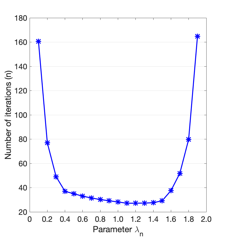
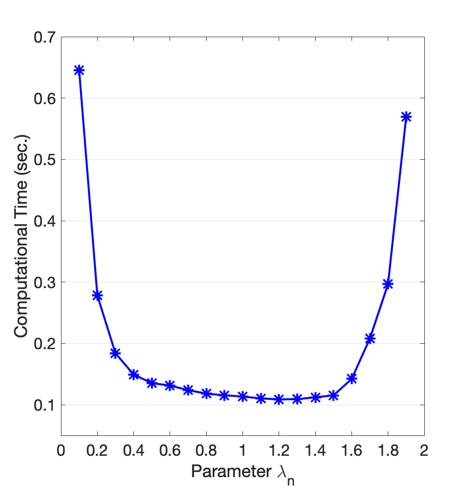
As it is well-known the the presence of an appropriate relaxation parameter λn∈(0,2)\lambda_{n}\in(0,2) in MECSPM, or even the state-of-the-art relaxation methods can make the methods converge faster. Now, we demonstrate the influence of the relaxation paramter λn\lambda_{n} when ESCoM-CGD is performed for solving the considered problem. We fix μ=10−4,φn=1(n+1)0.1\mu=10^{-4},\varphi_{n}=\frac{1}{(n+1)^{0.1}}, and βn=1(n+1)0.01\beta_{n}=\frac{1}{(n+1)^{0.01}}. We test a set of parameter λn∈{0.1,0.2,…,1.9}\lambda_{n}\in\{0.1,0.2,\ldots,1.9\}, and plot the number of iterations and computational time with respect to different choices of λn\lambda_{n} in Figure 4.

Refer to caption
Refer to caption
Figure 4: Influences of relaxation parameter λ\lambda when performing ESCoM-CGD.

According to the curves in Figure 4, we see that the relaxation paramter λn\lambda_{n} behaves significantly well convergence for a wide range of choices. In fact, we observe the the faster convergence is obtained for some intermediate choices of λn∈[0.8,1.5]\lambda_{n}\in[0.8,1.5], and the exactly best result is observed for λn=1.2\lambda_{n}=1.2. This observation relatively conforms to the numerical experiments in CN19.

Finally, to showcase the superiority of our ESCoM-CGD, we compare the methods for various size (m,k)(m,k) of randomly matrix 𝐀\mathbf{A}. We fix the corresponding parameters as in Table 2. To show performance of the methods, the number of iterations with respect to the size of 𝐀\mathbf{A} are plotted in Figure 5. Moreover, we also present computational time in seconds with respect to the sizes (m,k)(m,k) in Table 3.

Table 2: Best choice of parameters used for performing ESCoM-CGD, HCGM IY09 and HTCGM I11.
Parameter φn\varphi_{n} βn\beta_{n} μ\mu λn\lambda_{n}
ESCoM-CGD 1(n+1)0.1\frac{1}{(n+1)^{0.1}} 1(n+1)0.01\frac{1}{(n+1)^{0.01}} 10−410^{-4} 1.2
HCGM IY09 1(n+1)0.1\frac{1}{(n+1)^{0.1}} 1(n+1)0.5\frac{1}{(n+1)^{0.5}} 10−410^{-4} -
HTCGM I11 1(n+1)0.1\frac{1}{(n+1)^{0.1}} 1(n+1)0.5\frac{1}{(n+1)^{0.5}} 10−410^{-4} -
Refer to caption
Figure 5: Number of iterations when performing ESCoM-CGD, HCGM IY09 and HTCGM I11 for different choices of number of constraints (mm) and dimensions (kk).
Table 3: Computational time in seconds when performing ESCoM-CGD, HCGM IY09 and HTCGM I11 for different choices of number of constraints (mm) and dimensions (kk).
(m,k)(m,k) ESCoM-CGD HCGM IY09 HTCGM I11
(100,25) 0.0316 0.0375 0.0391
(300,75) 0.0621 0.0757 0.0699
(500,125) 0.1029 0.1370 0.1302
(700,175) 0.1499 0.1874 0.1758
(1000,250) 0.2045 0.2717 0.2557
(3000,750) 0.9660 1.2123 1.1694
(5000,1250) 2.2990 3.0666 3.0382
(7000,1750) 6.9761 9.2777 9.2878
(10000,2500) 25.3301 35.7751 35.4769
(20000,5000) 105.7223 143.8273 144.0225

The plots in Figure 5 show that ESCoM-CGD gives the best convergence results for all choices of (m,k)(m,k). Moreover, we see that HCGM and HTCGM reach the optimal tolerance at most the same number of iterations. Likewise, the results given in Table 3 reveal that ESCoM-CGD reaches the optimal tolerance faster than both HCGM and HTCGM. It is worth noting that when the size (20000,5000)(20000,5000), ESCoM-CGD requires computational time less than other two methods approximately 40 seconds. This underlines the essential superiority of the proposed ESCoM-CGD.

6 Conclusion

The object of this work was the solving of a variational inequality problem governed by a strongly monotone and Lipschitz continuous operator over the intersection of fixed-point sets of cutter operators. We associated to it the so-called extrapolated sequential constraint method with conjugate gradient direction. We proved strong convergence of the generated sequence of iterates to the unique solution to the considered problem. Our numerical experiments show that the proposed method has a better convergence behaviour compared to other two methods. For future work, one may consider and analyze a variant of the proposed method by using some constrained selections, e.g. the so-called dynamic string averaging procedure, for dealing with the constrained operators.

Acknowledgements.
Mootta Prangprakhon is partially supported by Science Achievement Scholarship of Thailand (SAST), and Faculty of Science, Khon Kaen University. Nimit Nimana is supported by Khon Kaen University.

References

  • (1) Bauschke, H.H., Combettes, P.L.: A weak-to-strong convergence principle for Fejér-monotone methods in Hilbert spaces. Math. Oper. Res. 26, 248–264 (2001)
  • (2) Bauschke, H.H., Combettes, P.L.: Convex analysis and monotone operator theory in Hilbert Spaces (2nd ed.) CMS Books in Mathematics, Springer, New York (2017)
  • (3) Bregman, L.M.: Finding the common point of convex sets by the method of successive projection. Dokl. Akad. Nauk SSSR. 162(3), 487–490 (1965)
  • (4) Cegielski, A.: Generalized relaxations of nonexpansive operators and convex feasibility problems. Contemp. Math. 513, 111–123 (2010)
  • (5) Cegielski, A.: Iterative methods for fixed point problems in Hilbert spaces. Lecture Notes in Mathematics 2057, Springer-Verlag, Berlin, Heidelberg, Germany (2012)
  • (6) Cegielski A., Censor, Y.: Opial-Type Theorems and the Common Fixed Point Problem. In: Bauschke H., Burachik R., Combettes P., Elser V., Luke D., Wolkowicz H. (eds.) Fixed-Point Algorithms for Inverse Problems in Science and Engineering. Springer Optimization and Its Applications, vol 49. Springer, New York, NY (2011)
  • (7) Cegielski, A., Censor, Y.: Extrapolation and local acceleration of an iterative process for common fixed point problems. J. Math. Anal. Appl. 394, 809–818 (2012)
  • (8) Cegielski, A., Nimana, N.: Extrapolated cyclic subgradient projection methods for the convex feasibility problems and their numerical behaviour. Optimization. 68, 145-161 (2019)
  • (9) Dai, Y.H., Yuan, Y.: A nonlinear conjugate gradient method with a strong global convergence property. SIAM J. Optim. 10, 177–182 (1999)
  • (10) Facchinei, F., Pang, J.-S.: Finite-dimensional variational inequalities and complementarity problems, volume I, Springer, New York (2003)
  • (11) Fletcher, R., Reeves, C. M.: Function minimization by conjugate gradients. Comput. J. 7, 149–154 (1964)
  • (12) Gilbert, J.C., Nocedal, J.: Global convergence properties of conjugate gradient methods for optimization. SIAM J. Optim. 2, 21–42 (1992)
  • (13) Goldstein, A.A.: Convex programming in Hilbert space. Bull. Amer. Math. Soc. 70, 709–710 (1964)
  • (14) Iiduka, H.: Three-term conjugate gradient method for the convex optimization problem over the fixed point set of a nonexpansive mapping. Appl. Math. Comput. 217, 6315–6327 (2011)
  • (15) Iiduka, H.: Fixed point optimization algorithms for distributed optimization in networked systems. SIAM J. Optim. 23, 1–26 (2013).
  • (16) Iiduka, H.: Convex optimization over fixed point sets of quasi-nonexpansive and nonexpansive mappings in utility-based bandwidth allocation problems with operational constraints. J. Comput. Appl. Math. 282, 225–236 (2015)
  • (17) Iiduka, H.: Acceleration method for convex optimization over the fixed point set of a nonexpansive mapping. Math. Program. 149, 131–165 (2015)
  • (18) Iiduka, H.: Distributed Optimization for Network Resource Allocation With Nonsmooth Utility Functions. IEEE Trans. Control. Netw. Syst. 6, 1354–1365 (2019)
  • (19) Iiduka, H.: Stochastic fixed point optimization algorithm for classifier ensemble. IEEE Trans Cyber. (Early Access). DOI: 10.1109/TCYB.2019.2921369.
  • (20) Iiduka, H., Hishinuma, K.: Acceleration method combining broadcast and incremental distributed optimization algorithms. SIAM J. Optim. 24, 840–1863 (2014)
  • (21) Iiduka, H., Yamada, I.: A use of conjugate gradient direction for the convex optimization problem over the fixed point set of a nonexpansive mapping. SIAM J. Optim. 19, 1881–1893 (2009)
  • (22) Kaczmarz, S.: Angenäherte Auflösung von Systemen linearer Gleichungen, Bull. inter. A35, 355–357 (1937); English translation: Kaczmarz, S.: Approximate solution of systems of linear equations. Int. J. Contr. 57, 1269–1271 (1993)
  • (23) Liu, C.: An acceleration scheme for row projection methods. J. Comput. Appl. 57, 363–391 (1995)
  • (24) Nocedal, J., Wright, S.J.: Numerical Optimization. Springer, Springer Series in Operations Research and Financial Engineering, Berlin (1999)
  • (25) Opial, Z.: Weak convergence of the sequence of successive approximations for nonexpansive mappings. Bull. Amer. Math. Soc. 73, 591-597 (1967)
  • (26) Xu, H.K.: Iterative algorithm for nonlinear operators. J. London Math. Soc. 66, 240–256 (2002)
  • (27) Yamada, I.: The hybrid steepest descent method for the variational inequality problem over the intersection of fixed point sets of nonexpansive mappings. In: Butnariu, D., Censor, Y., Reich S. (eds.) Inherently Parallel Algorithms in Feasibility and Optimization and their Applications. Elsevier, Amsterdam, 473–504 (2001)
  • (28) Zarantonello, E.H.: Projections on convex sets in Hilbert space and spectral theory. in: Zarantonello, E.H. (Ed.) Contributions to Nonlinear Functional Analysis. Academic Press, NewYork, NY, USA, 237–424 (1971)
  • (29) Zhang, L., Zhou, W., Li, D.H.: A descent modified polak-ribiere-polyak conjugate gradient method and its global convergence. IMA J. Numer. Anal. 26, 629–640 (2006)
  • (30) Zhang, L., Zhou, W., Li, D.H.: Global convergence of a modified fletcher-reeves conjugate gradient method with Armijo-type line search. Numer. Math. 104, 561–572 (2006)
  • (31) Zhang, L., Zhou, W., Li, D.H.: Some descent three-term conjugate gradient methods and their global convergence. Optim. Methods Softw. 22, 697–711 (2007)