Improved phase-field models of melting and dissolution in multi-component flows
Abstract
We develop and analyse the first second-order phase-field model to combine melting and dissolution in multi-component flows. This provides a simple and accurate way to simulate challenging phase-change problems in existing codes. Phase-field models simplify computation by describing separate regions using a smoothed phase field. The phase field eliminates the need for complicated discretisations that track the moving phase boundary. However standard phase-field models are only first-order accurate. They often incur an error proportional to the thickness of the diffuse interface. We eliminate this dominant error by developing a general framework for asymptotic analysis of diffuse-interface methods in arbitrary geometries. With this framework we can consistently unify previous second-order phase-field models of melting and dissolution and the volume-penalty method for fluid-solid interaction. We finally validate second-order convergence of our model in two comprehensive benchmark problems using the open-source spectral code Dedalus.
1 Introduction
Many scientific and industrial questions involve fluid flows coupled with phase changes; including sea-ice formation [19], semiconductor crystal manufacture [26], binary alloy solidification [14], and geophysical mantle dynamics [30]. Multi-phase interaction combines the challenges of nonlinear multi-component convection [56] and evolution of phase boundaries [35], creating entirely new effects. Quantifying this complexity demands appropriate mathematical tools.
Moving boundary problems are the standard method to model phase change phenomena. Separate partial differential equations (PDEs) exist in the liquid and solid regions and moving boundary conditions are applied at the interface (see fig. 1 ). A dynamically shifting interface means that the boundary conditions form an essential (often nonlinear) part of the solution [63]. Moving boundaries present many challenges, complicating numerical algorithms [18] and mathematical proofs [27].
As a possible remedy, it is useful to recall that boundary conditions are a mathematical abstraction; they result from limiting cases of rapid transitions in material properties. There is a long history of reinterpreting discontinuous boundary conditions as smoothed phenomena. Where Gibbs treated capillarity with infinitesimal surfaces [25], Van der Waals understood the importance of smoothness at phase boundaries [58]. Where Stefan treated solid-liquid phase boundaries as discontinuous [51], Cahn and Hilliard modelled phase separation as smoothed [14]. Readopting a physics-based viewpoint of boundary conditions allows new possible techniques for addressing complex multi-phase problems. As well as providing a firmer mathematical and physical foundation, smoothed models also simplify numerical implementations by removing the need to track the infinitesimal boundary.
This paper focusses on phase-field models, one of the foremost examples of this smoothed approach. Phase-field models represent distinct phases using a single smoothed phase field , illustrated in fig. 1 [6, 52]. The evolution of the phases is then determined by a single set of equations that apply over the entire domain. Many other methods also model phase changes, such as enthalpy methods [59, 57], level set methods [47, 15], diffuse-domain approaches [39, 1], or some immersed-boundary methods [42]. Yet phase-field models stand out for combining several key benefits:
- •
- •
- •
- •
- •
- •
We emphasise this last point. The simulation of moving boundary problems requires specialised algorithms designed to track and apply boundary conditions at the interface. These algorithms can be difficult or impossible to implement in existing codes. For example, spectral methods are popular for their efficiency, but cannot easily handle non-trivial geometries or topologies. Phase-field models (and other diffuse-interface methods) alleviate these difficulties by removing boundary conditions from the problem formulation. By replacing boundary conditions with simple source terms, they can be implemented in general codes for little effort. More general effects can be modelled by changing source terms, as opposed to developing and integrating new algorithms into the codebase. Phase-field models extend the range of phenomena that existing codes can simulate, and accelerate the development of codes to study new scientific problems.
However, phase-field models possess one important drawback for simulation: they must resolve the diffuse interface. For small-scale simulations this is feasible. But there is a vast disparity between the microscopic scale of the smoothed interface and the macroscopic scale of interest in most problems. This disparity is what makes discontinuous boundary conditions appropriate models in most circumstances. Throughout this paper, we denote this ratio by
| (1) |
Numerically feasible values of are orders of magnitude larger than reality. Straightforward analysis implies a commensurate error with respect to the limiting boundary conditions.
The only way to perform accurate phase-field simulations with achievable values of is to accelerate the convergence of the model itself. This can be done through second-order asymptotic analysis in the limit . While the first order is sufficient to determine the limiting behaviour, it is the second order that reveals the dominant error of the model. It is then possible to find optimal prescriptions that cancel the dominant error and boost convergence from to .
This strategy leads to various ‘quantitative’ (i.e. second-order) phase-field models, beginning with a correction for arbitrary interface-kinetics in pure materials [33, 34], and since extended to unequal diffusivities [2, 43], multiple components [32], and the combination thereof [24, 45]. An introduction to this asymptotic procedure can be found in [22]. Despite much success, progress is difficult. Second-order asymptotic analysis has not yet ascertained a quantitative phase-field model of multi-component convection11 1 Shortly before submission we became aware of the work [53]. In it, Subhedar et al. perform second-order analysis of a phase-field model combining melting and advection. Our work is more general as we also account for dissolution, give a more comprehensive analytical treatment, and use more challenging computational benchmarks..
This paper presents the first second-order phase-field model of buoyancy-forced convecting binary mixtures. The model, given in section 2, builds on first-order models of multicomponent convection [4], second-order models of pure melts [16], the diffuse domain method for Robin boundary conditions [36], and the smooth volume-penalty method for no-slip boundary conditions [28]. We verify second-order convergence in section 3 by developing a straightforward asymptotic procedure suitable for general equations and geometries in three dimensions. This procedure allows us to consistently analyse and unify previous second-order phase-field and diffuse-interface methods. We also implement this procedure in the symbolic computing language Mathematica. For brevity we assume somewhat simplified thermodynamical properties in our model, such as uniform temperature diffusivity, negligible solute within the solid, and Boussinesq buoyancy. Each assumption could be relaxed and analysed using the framework of section 3. We finally validate the improved convergence in two comprehensive benchmark problems implemented in the Dedalus numerical code [9] in section 4.
2 Models of melting in binary mixtures
2.1 Conventional moving boundary formulation
Melting in binary mixtures, such as ice in sea water, is often modelled as a moving boundary problem. We partition the domain into fluid and solid regions, pose separate PDEs on each subdomain, and apply boundary conditions at the evolving interface (as in fig. 1 (a)).
In the fluid, the temperature and dissolved solute concentration satisfy advection-diffusion equations, and the fluid velocity and pressure satisfy incompressible Navier-Stokes equations with Boussinesq buoyancy forcing ,
| (2) |
where and are the thermal, solutal, and momentum diffusivity (each assumed constant), and , , and are the gravitational acceleration, the density of the fluid, and a reference density. In the solid only the temperature is defined, which follows a diffusive equation,
| (3) |
We require several boundary conditions at the moving interface [63]. The Gibbs-Thompson relation relates departure of thermosolutal equilibrium (, where is the liquidus slope) to a mean-curvature dependent surface energy, and kinetic undercooling proportional to the interfacial normal velocity . The Stefan condition expresses heat conservation, equating latent heat release with a discontinuity in temperature flux. The Robin concentration condition ensures total solute conservation. Zero velocity boundary conditions maintain mass conservation,
| (4) |
This model involves several idealisations, namely Boussinesq buoyancy forcing, constant diffusivities and densities that are phase, temperature, and concentration invariant, and a linear liquidus relation. We can include more general thermodynamic properties into our framework, but we continue with the current model as it captures many aspects of melting and dissolution in multi-component flows. Kinetic undercooling is only relevant for rapidly solidifying supercooled liquids so we set . Note that the neglect of density change during melting means the fluid velocity is equal to zero at the moving interface.

2.2 Phase-field model
Phase-field models represent an alternative approach that is physically motivated and simple to simulate. They represent distinct phases with a smoothed phase field . This field obeys an Allen-Cahn type equation which forces the phase to in the solid and in the fluid [4]. The interface is represented implicitly by the level set . The new equations augment are,
| (5) |
The new source terms of section 2.2 can be understood heuristically. At leading order, the phase-field equation develops a tanh-like profile around the interface with thickness . Beyond this distance the phase tends to its limiting values of zero in the fluid and one in the solid. In the fluid section 2.2 reproduces section 2.1. in the solid the advective and diffusive solute flux tend to zero (with regularising the concentration equation for numerical stability), and the velocity is damped by Darcy drag terms for porous media. At next order thermosolutal forcing perturbs the interface to generate latent heat. For a clear derivation of a similar first-order model see [4].
Our goal is to surpass this approximate understanding and demonstrate improved convergence of this optimised phase-field model to the original moving boundary formulation. We achieve this with an asymptotic analysis of section 2.2 as the interface length-scale tends to zero. Proving these equations converge to the moving boundary formulation at in general geometries is nontrivial, but builds on second-order models of each individual boundary condition; a phase-field model which optimises the mobility term for zero interface kinetics [16], a concentration equation similar to [4] and the diffuse domain method for Robin boundary conditions [36], and the smooth volume penalty method (which gives ) [28].
3 Analysis of the phase-field model
In order to understand the phase-field model and demonstrate second-order accuracy we use a multiple-scales matched-asymptotics framework, which we break into several modular steps:
- 1.
Partition the solid , fluid , and size boundary regions (fig. 1 ).
- 2.
Adopt signed distance coordinates in the boundary region (section 3.1.1, fig. 1 ).
- 3.
Rescale normal coordinate and operators by near the interface (section 3.1.2, fig. 1 ).
- 4.
Expand the variables in an asymptotic power series in in each region (section 3.1.3).
- 5.
Connect regions with asymptotic matching conditions in the limit (section 3.1.4).
- 6.
Iterate to solve the zeroth, first, and second order problems (sections 3.2, 3.3 and 3.4).
This procedure follows our previous analysis of the volume-penalty method [28]. The philosophy of our approach is to determine the evolution of the phase-field model up to and including in each region. We show that the variables in the fluid and solid regions, as well as the location of the interface itself, evolve with only divergence from the moving boundary formulation. Errors of in the temperature and tangential velocity do occur in the boundary region . But this deviation is a necessary consequence of smoothly approximating discontinuous gradients across the interface, and is localised to the boundary region. We thereby derive a second-order accurate phase-field model. We now summarise the key components of this procedure22 2 We also provide a Mathematica script that automates each step of this analysis at github.com/ericwhester/phase-field-code..
3.1 Summary of asymptotic procedure
3.1.1 Signed-distance coordinate system
We build a simple orthogonal coordinate system in the boundary region using the signed-distance function from the level set. The signed distance is the minimum distance of a point to the interface. It follows that the point must lie in the direction of the unit normal vector from the nearest point on the interface , which we label with surface coordinates ,
| (6) |
The surface coordinates induce a tangent vector basis . Given orthogonal surface coordinates, we also derive the dual vector basis and a unique orthonormal tangent basis ,
| (7) |
We can then write the surface area measure and surface gradient ,
It is not difficult to show the normal is everywhere equal to the gradient of the signed distance. The gradient of the normal is therefore symmetric and diagonalisable. The eigenvectors are the principal directions of curvature (which must align with orthogonal surface coordinates), and the eigenvalues are the principal curvatures ,
| (8) |
We use this orthonormal frame to describe all geometric quantities near the interface. We can then express the gradient using the surface and normal derivatives and the scale tensor
| (9) |
It is straightforward to derive the remaining vector calculus operators from the gradient, which we list in appendix A. Finally, the Cartesian partial time derivative can be rewritten in a moving coordinate system using the signed-distance partial time derivative ,
| (10) |
3.1.2 Rescaling interfacial coordinates
We analyse the size interfacial region using the rescaled coordinate and derivative ,
| (11) |
This rescales vector calculus operators (listed in appendix A) through scale factors of the gradient
| (12) |
3.1.3 Variable expansions with formal power series
After splitting the domain into the fluid , solid , and interfacial regions, each variable in each region (fluid , solid , and interfacial ) is expressed as a power series in ,
| (13) |
We do so for the temperature , solute concentration , fluid velocity , pressure , phase field , and interface velocity (which does not depend on ). We substitute these series into the hierarchy of equations generated by section 3.1.2 to derive a system of equations at each order of . Solving each order requires a matching procedure between adjacent regions.
3.1.4 Asymptotic matching
To ensure agreement between different regions we specify asymptotic matching boundary conditions. This subtle notion requires asymptotic agreement in intermediate zones in the limit that . We can then let approach infinity for the inner problem without encountering coordinate singularities (provided ), and let approach zero for the outer problem without entering the interfacial region. That is, for any variable , we require
| (14) |
Each variable is already expressed as an asymptotic series. Each series term in the outer variables can be further expanded as a Taylor series about the interface at using the signed distance . The matching conditions at each order of then simplify to
| (15) |
| Equipped with our multiple-scales matched-asymptotics procedure, we can now verify second-order convergence of our phase-field model in general smooth geometries. |
3.2 Zeroth order
At leading order the phase-field equation reduces to the condition . We define the solid by , the liquid by , with the boundary region separating them.
Fluid problem — Noting that the phase is zero in the fluid, we recover the desired sharp interface equations for the remaining leading order variables,
For brevity we approximate the buoyancy relationship as being linear in temperature and concentration, with proportionality constants and respectively. This simplification does not affect the convergence results. The solutions may also require external boundary conditions to complete the system.
Solid problem — Within the solid, we reproduce the diffusion equation for the temperature, and zero velocity in the solid. The divergence of the momentum equation reveals a Poisson equation for the pressure. The concentration equation depends sensitively on the decay of the phase to zero, but in the region the concentration forcing terms vanish, giving
Similarly, internal ice boundary conditions may be necessary.
Boundary problem — The boundary region is defined relative to the interface . To hold true for all when expanded into its power series, this implies that
In this region the phase-field equation balances the diffusion and reaction terms. The limiting boundary conditions and imply a tanh profile for ,
Matching the inner heat equation to the outer temperature requires to be constant in ,
The identity simplifies the concentration equation. The limiting behaviour of the operator implies exponential growth of the kernel into the solid. This is unphysical, implying that the operand is zero. Matching to the outer variables requires a constant concentration,
The divergence constraint and matching to the solid implies zero normal velocity,
The tangential momentum equation balances diffusion with damping. The kernel is spanned by an unphysical solution that grows exponentially into the solid, and a physical solution that decays exponentially into the solid and is affine in the fluid. Calibrating [28] allows linear (rather than affine) behaviour in the fluid. Matching to the fluid implies is zero,
In summary, the zeroth order asymptotics shows that the phase field has a tanh profile near the boundary, and that the leading order outer velocities satisfy no-slip boundary conditions. The next order problem reproduces the remaining boundary conditions.
3.3 First order
The first-order perturbation of the phase-field equation away from the interface takes the form
At subsequent orders the leading order operator pairs with the highest order . The forcing terms contain lower order factors. As the first inhomogeneity is zero all remaining forcing terms, and therefore all outer phase-field expansions , are zero.
Fluid problem — The remaining fluid equations are linear and homogeneous,
The external boundary conditions are satisfied by the zeroth order outer solutions. The first-order corrections therefore have homogeneous external boundaries. They are only perturbed at the melting interface. We show this interfacial perturbation is zero at first order.
Solid problem — The solid equations are the same at first order,
Boundary problem — The differential operator of the first-order phase-filed equation has a two dimensional kernel spanned by and . The inhomogeneity must be orthogonal to the kernel, implying the Gibbs-Thomson condition,
Matching implies . Integrating the temperature equation recovers energy conservation,
Solving the homogeneous concentration equation and matching gives the solute conservation condition,
The divergence condition when matched with the solid again implies zero normal velocity,
The tangential velocity is proportional to the physical solution . We choose [28] to ensure linear behaviour in the fluid,
We finally use the normal momentum equation to show the pressure is constant at leading order
The first-order asymptotics have reproduced the Gibbs-Thomson condition with zero interface kinetics and the solute and energy conservation boundary conditions. Hence the phase-field equations will tend to the sharp interface equations in the limit. Calibrating ensures the first-order outer fluid velocity satisfies homogeneous boundary conditions . We now solve the second-order asymptotics to show that the mobility coefficient ensures homogeneous boundary conditions for the first-order outer temperature and concentration, and that the first-order interfacial velocity error is zero — allowing second-order convergence.
3.4 Second order
Fluid problem — At second order the fluid equations are sourced by the first-order errors,
Solid problem — The solid velocity is now non-zero from interior pressure and forces,
Boundary problem — The phase-field equation now has a more complex inhomogeneous term.
We again apply a solvability condition. The odd terms drop out, and integration shows and . The interfacial velocity term thus vanishes, giving a constraint between first-order concentration and temperature.
An explicit formula for (using variation of parameters) is non-trivial but it decays exponentially to zero in either direction. The temperature equation is then integrated. If initially , then matching prevents linear asymptotic behaviour of , implying ,
The concentration equation is similarly integrated. The inhomogeneity is constant in , and explicitly solvable. Using previous solutions and , we find ,
The divergence equation implies the second-order normal velocity is now no longer zero,
The second-order tangential velocity can then be solved using variation of parameters
where is a constant of integration that cancels the linear part of the solution into the fluid. The normal momentum equation can then be integrated to determine . Matching requires no constant term in the limiting behaviour of the pressure into the fluid,
The second-order asymptotic analysis shows that calibrating the mobility and damping parameters ensures homogeneous boundary conditions of the first-order outer solutions at the interface. Combined with homogeneous external boundary conditions and homogeneous linear evolution equations at first order, this implies that if the outer solutions are initialised correct to , then the fields and interfacial velocity will evolve accurate to over time. In reality the chaotic nature of many fluid dynamics problems prevents convergence beyond the Lyapunov timescale of the flow, but at each point in time the system behaves correctly to within second-order accuracy.
4 Numerical validation of the model
We now validate the asymptotic arguments of section 3 in two benchmark problems. In each problem we calculate a numerical reference solution corresponding to the “sharp interface” equations of section 2.1. We then show the optimal phase-field equations of section 2.2 achieve convergence of to these reference solutions. Both the reference and phase-field problems are simulated using the flexible and efficient spectral code Dedalus [9]33 3 The full simulation code, saved data, and analysis scripts are freely available at github.com/ericwhester/phase-field-code.. This allows us to probe equation-level model error in the absence of numerical discretisation errors.
4.1 Melting and dissolution at a stagnation point
The first benchmark problem examines warm liquid with dissolved solute flowing toward a melting interface at a stagnation point, (similar to section 5 of [38] and 5.6 of [28]). We compare the sharp interface and phase-field approximations to this problem, as illustrated in fig. 2. The symmetries of the system allow us to significantly simplify section 2.1, revealing a steady travelling wave similarity solution for the moving boundary and phase-field formulations. We do this by transforming to a frame moving leftward at the steady interface melting speed . We solve the system as a nonlinear boundary value problem in Dedalus.
Sharp interface model — We solve a diffusion equation for the solid temperature , advection-diffusion equations for the liquid temperature and solute concentration , and a nonlinear third order equation for the horizontal fluid velocity ,
| (17) |
Note that though we solve in the moving frame, we do not apply a Galilean boost to the fluid velocity. These equations must also satisfy energy conservation, solute conservation, temperature continuity and Gibbs-Thomson relations at the liquid-solid interface, and Dirichlet conditions at . We can then solve for each variable and the unknown melting speed .
| (18) |
Phase-field model — The phase field instead implicitly models the interfacial boundary conditions through various equation terms, which reduce section 2.2 to,
| (19) |
We now only require the Dirichlet outer boundary conditions of before to solve the problem
| (20) |
Requiring is necessary to fix the problem in the moving frame to determine .

Results — We solve each problem as a nonlinear boundary value problem in Dedalus. We discretise each variable on the solid () and fluid () domains using Chebyshev polynomials. Newton-Kantorovich iteration then converges on a solution with a tolerance of (see [8] appendix C). We reproduce example phase field and reference snapshots in fig. 2 for , , and , using 64 grid points for each subdomain. We set to regularise the solute equation within the solid. The disagreement (though small) is visible by eye for the temperature, concentration, and normal velocity.
We then perform a quantitative analysis of convergence in fig. 3. We test seven logarithmically spaced values of from to , for the previous control parameters, and using 256 grid points in each subdomain. We quantify the difference between the reference and phase-field solutions with the and error norms of each variable as a function of . We find clear convergence in the error norm of each field variable, as well as for the error norm of the , and variables. The convergence demonstrates the quantitative accuracy of the phase-field model. The reason for the apparently restricted convergence of the temperature fields is the jump in temperature gradient of the reference solution at the interface. The smooth phase-field model cannot follow this kink leading to an disagreement that is localised to the boundary. Tangential velocities also suffer from this reduced continuity in general.
4.2 Double diffusive melting
In our second benchmark we examine buoyancy driven flow of warm liquid with dissolved solute underneath a melting solid layer. This problem develops nontrivial geometries from the evolution of the flow. To simulate the reference formulation in Dedalus, we use an evolving coordinate system that maps the fluid and solid regions to a stationary rectangular domain. This transformation allows an efficient spectral discretisation using Dedalus, and is used in similar spectral solvers [54]. We repeat this remapping for the phase-field formulation as it concentrates resolution near the level set. This allows us to efficiently and accurately simulate much smaller . By comparing the phase-field simulation to the reference problem as we decrease , we demonstrate second-order accuracy of the model.
Sharp differential equations — The full domain exists between and . It is partitioned by the interface at height . Above the interface we solve the heat equation for the solid temperature field with diffusivity . Below the interface we solve incompressible Boussinesq hydrodynamics (using a first-order formulation in terms of velocity , vorticity , and augmented pressure ), with advection and diffusion of temperature and solute concentration ,
| (21) |
where and are the momentum, temperature, and solute diffusivity. This first-order reformulation is required in the Dedalus solver, and has the added benefit of simplifying the mathematical details of the coordinate transformation. We set the buoyancy parameter .
Boundary conditions — At the top we specify conservative temperature boundary conditions. At the bottom, we specify no-slip boundaries with no-flux temperature and solute conditions. The zeroth mode for the vertical velocity is replaced by a choice of pressure gauge,
At the interface , we have a Gibbs-Thomson boundary condition, matching temperature boundary conditions, energy and solute conservation boundary conditions, and zero velocity boundary conditions required for mass conservation,
| (22) |
Initial conditions — We initialise the problem with and zero velocity and pressure, and a decreasing concentration profile with height. We apply a large perturbation to the linearly decreasing temperature field to initiate convection,
Phase-field equations — The phase-field equations are a similar reformulation of section 2.2.
We use the optimal damping prescription [28] and choose . We specify the same insulating no-slip boundary conditions at and . The boundary conditions at require continuity of each field and its derivatives. We initialise using the same initial conditions as for the remapped simulation, plus the initial conditions for the phase field
Remapped coordinates — To solve the melting problem we remap our evolving domain in Cartesian space to a fixed rectangular domain with the new coordinates and ,
for which we plot equally spaced level set contours in fig. 4. The differential geometry of the new coordinates is presented in appendix B. We solve the phase field equations on the remapped domains of the reference problem to concentrate resolution near the phase-field interface and speed up comparison of quantities between simulations.
Model and numerical parameters — We simulate these equations using model parameter values from table 1. We simulate the reference equations using 64 Chebyshev polynomials in the vertical direction and 128 Fourier modes in the periodic horizontal direction. After determining the reference solution, we discretise the phase-field equations on the same evolving domain of the reference simulation for several values of . To interpolate the reference geometries into the phase-field simulations between the saved time and grid points we use third order interpolating splines. The phase-field simulations discretise the vertical basis using three compound Chebyshev bases , with resolutions of 32, 64, and 32 modes respectively. This greatly reduces the simulation cost. We use a time step size of for decreasing choice of , and integrate in time using a second-order multistep semi-implicit backwards difference formula (SBDF2).
| 1 | 0.2 | 0 |
Results — A time series of the temperature and concentration fields of the reference solution is given in fig. 6, which illustrates a rising buoyant plume from the initial temperature anomaly in the fluid. The warm solute-laden liquid melts the interface in the middle more rapidly than the ambient liquid at the sides, causing a trough to develop.
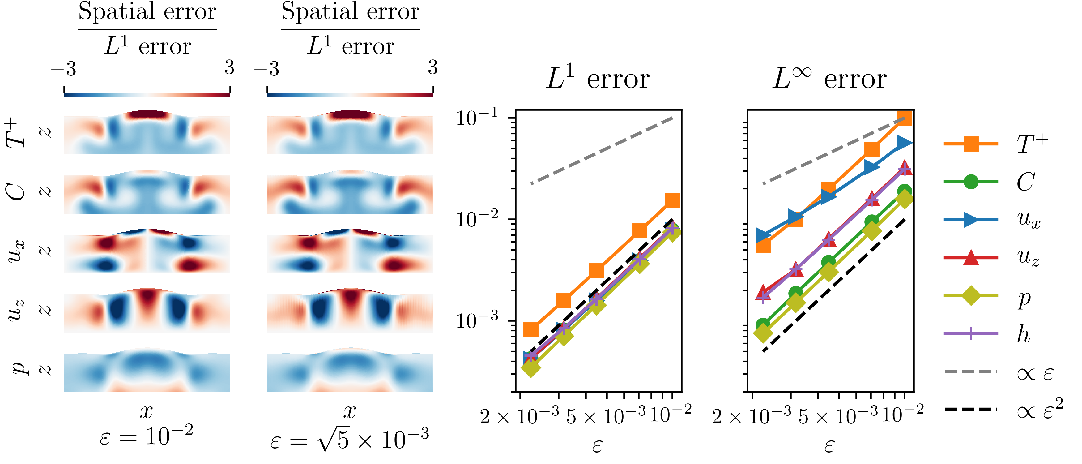
In fig. 6 we plot several error metrics of the phase-field simulations. In the first two columns we plot the spatial error normalised by the error for the liquid temperature , solute concentration , Cartesian velocity components and , and true pressure . We plot these normalised spatial errors for the smoothest () and sharpest () phase-field simulations at the final time . These plots reveal a consistent spatial error profile between simulations. To understand the amplitude of the spatial error, we plot the and error norms of each variable as a function of in the third and fourth columns of fig. 6. We see clear second-order convergence of all variables in norm. We note that the structure of the boundary layer of the tangential velocity and temperature affects error norm. The phase-field model causes a kink in the temperature and tangential velocity near the interface, which leads to an error of these variables in the interfacial region. However, this error is localised to the boundary, and does not propagate outward. (This trend is difficult to notice in the temperature plot as the error within the fluid still dominates the boundary error for the moderate choices of chosen.) We therefore achieve second-order convergence in the fluid and solid regions due to our optimal calibration of the phase-field model parameters.

5 Conclusions
In this paper we provide a general framework for analysing the convergence of phase-field models. We use this procedure to develop a second-order phase-field model of melting and dissolution in multi-component flows. This is a concrete advancement that showcases second-order accurate approximations of many common boundary conditions; no-slip Dirichlet boundaries, Neumann boundaries, Robin boundaries, and Stefan boundaries. We also verify these prescriptions in two thorough benchmark problems with accurate reference solutions. By developing a framework to validate this model, we now possess the machinery requied to create second-order accurate extensions to more general thermodynamic properties. We can also consider yet higher order analyses of this and other models. An automated approach of Richardson sequence extrapolation could also be considered to generate higher order accurate models, as was done by the authors for the volume-penalty method [28]. To be clear, phase-field models are not necessarily the most appropriate choice for any problem. Remapping was also shown to be an effective strategy for sufficiently simple geometries in section 4.2. However our second-order phase-field model is simple to implement, is more accurate than standard phase-field models, and is applicable in much more challenging geometries than remapping approaches.
Appendix A Signed-distance coordinates
The signed distance of the point is the minimum distance to the surface. Labelling surface points and unit normals with orthogonal surface coordinates , we have
This gives a tangent vector basis , dual basis , and orthonormal tangent basis .
These give the surface gradient , area measure , and surface divergence,
The normal is everywhere equal to the gradient of the signed distance, and is therefore its gradient is symmetric and diagonalisable. The eigenvectors are the principal directions of curvature (which align with orthogonal surface coordinates), and the eigenvalues are the principal curvatures ,
We express the gradient using the orthonormal frame and the scale tensor
We now give the remaining geometric quantities needed for all vector calculus operations. The determinant relates mean curvature , Gaussian curvature , and volume measure ,
We define the adjugate tensors and ,
We also define the cross product with the unit normal, which admits simple identities,
We next find the gradient of the basis vectors, and define Ricci rotation coefficients,
These relations allow us to calculate all relevant vector calculus operators,
Rescaling — Rescaling the normal coordinate by gives the following operators:
Appendix B Differential geometry of remapped coordinates
We solve section 4.2 by remapping to a fixed rectangular domain with coordinates and ,
where is the interface height in the new coordinates. We now develop the differential geometry required to write section 2.1 and section 2.2 in the new coordinates. We give explicit formulae for the remapping. The remapping is analogous and straightforward to derive. We use a tangent vector basis derived from the Jacobian of our transformation and its inverse ,
The tangent vector components are the rows of the spatial component of the inverse Jacobian . We use Einstein notation to sum over the spatial indices . These tangent vectors induce dual vectors which satisfy , with components from the column vectors of the spatial component of the Jacobian. We record the length of the vectors using the metric, with co/contravariant components , ,
These give “Jacobian” determinants of . The completely antisymmetric tensor can be transformed from Cartesian coordinates,
where is the antisymmetric symbol. We project the gradient to the tangent basis with the covariant derivative . We measure spatial variation of the basis with the connection coefficients . For the tangent basis, the connection coefficients take a particularly simple and symmetric form
We note the connection coefficients for the dual vectors are related to those for the tangent basis by . The partial time derivative changes as defined in zeroth row of the Jacobian, and the basis vectors also evolve in time,
These geometric quantities allow us to calculate all the relevant vector calculus quantities,
The normal vector at the interface is proportional to the dual vector. This gives us the normal gradient and normal velocity at the interface,
We finally write the interfacial curvature as . This completes the relations used to simulate the sharp interface and phase-field equations in remapped geometries.
References
- [1] S. Aland, J. Lowengrub, and A. Voigt, Two-phase flow in complex geometries: A diffuse domain approach, Computer modeling in engineering & sciences : CMES, 57 (2010), pp. 77–106.
- [2] R. F. Almgren, Second-Order Phase Field Asymptotics for Unequal Conductivities, SIAM Journal on Applied Mathematics, 59 (1999), pp. 2086–2107.
- [3] D. M. Anderson, G. B. McFadden, and A. A. Wheeler, A phase-field model of solidification with convection, Physica D: Nonlinear Phenomena, 135 (2000), pp. 175–194.
- [4] C. Beckermann, H. J. Diepers, I. Steinbach, A. Karma, and X. Tong, Modeling Melt Convection in Phase-Field Simulations of Solidification, Journal of Computational Physics, 154 (1999), pp. 468–496.
- [5] Z. Bi and R. F. Sekerka, Phase field model of solidification of a binary alloy, Physica A, (1998), p. 12.
- [6] W. J. Boettinger, J. A. Warren, C. Beckermann, and A. Karma, Phase-Field Simulation of Solidification, Annual Review of Materials Research, 32 (2002), pp. 163–194.
- [7] P. Bollada, P. Jimack, and A. Mullis, Bracket formalism applied to phase field models of alloy solidification, Computational Materials Science, 126 (2017), pp. 426–437.
- [8] J. P. Boyd, Chebyshev and Fourier Spectral Methods: Second Revised Edition, Courier Corporation, Dec. 2001.
- [9] K. J. Burns, G. M. Vasil, J. S. Oishi, D. Lecoanet, and B. P. Brown, Dedalus: A flexible framework for numerical simulations with spectral methods, Physical Review Research, 2 (2020), p. 023068.
- [10] G. Caginalp, An analysis of a phase field model of a free boundary, Archive for Rational Mechanics and Analysis, 92 (1986), pp. 205–245.
- [11] G. Caginalp, Stefan and Hele-Shaw type models as asymptotic limits of the phase-field equations, Physical Review A, 39 (1989), pp. 5887–5896.
- [12] G. Caginalp and X. Chen, Convergence of the phase field model to its sharp interface limits, European Journal of Applied Mathematics, 9 (1998), pp. 417–445.
- [13] G. Caginalp and P. Fife, Dynamics of Layered Interfaces Arising from Phase Boundaries, SIAM Journal on Applied Mathematics, 48 (1988), pp. 506–518.
- [14] J. W. Cahn and J. E. Hilliard, Free Energy of a Nonuniform System. I. Interfacial Free Energy, The Journal of Chemical Physics, 28 (1958), pp. 258–267.
- [15] S. Chen, B. Merriman, S. Osher, and P. Smereka, A Simple Level Set Method for Solving Stefan Problems, Journal of Computational Physics, 135 (1997), pp. 8–29.
- [16] X. Chen, G. Caginalp, and C. Eck, A rapidly converging phase field model, Discrete and Continuous Dynamical Systems, 15 (2006), pp. 1017–1034.
- [17] L.-A. Couston, E. Hester, B. Favier, J. R. Taylor, P. R. Holland, and A. Jenkins, Ice melting in a turbulent stratified shear flow, arXiv:2004.09879 [physics], (2020).
- [18] J. Donea, A. Huerta, J.-P. Ponthot, and A. Rodríguez-Ferran, Arbitrary Lagrangian–Eulerian Methods, in Encyclopedia of Computational Mechanics, American Cancer Society, 2004, ch. 14.
- [19] M. Epstein and F. B. Cheung, Complex Freezing-Melting Interfaces in Fluid Flow, Annual Review of Fluid Mechanics, 15 (1983), pp. 293–319.
- [20] M. Fabbri and V. R. Voller, The Phase-Field Method in the Sharp-Interface Limit: A Comparison between Model Potentials, Journal of Computational Physics, 130 (1997), pp. 256–265.
- [21] B. Favier, J. Purseed, and L. Duchemin, Rayleigh–Bénard convection with a melting boundary, Journal of Fluid Mechanics, 858 (2019), pp. 437–473.
- [22] P. C. Fife, Dynamics of Internal Layers and Diffusive Interfaces, no. 53 in CBMS-NSF Regional Conference Series in Applied Mathematics, Society for Industrial and Applied Mathematics, Philadelphia, Pa, 1988.
- [23] G. J. Fix, Phase field methods for free boundary problems, (1982).
- [24] H. Garcke and B. Stinner, Second order phase field asymptotics for multi-component systems, Interfaces and Free Boundaries, (2006), pp. 131–157.
- [25] J. W. Gibbs, On the equilibrium of heterogeneous substances, American Journal of Science, s3-16 (1878), pp. 441–458.
- [26] M. E. Glicksman, S. R. Coriell, and G. B. McFadden, Interaction of Flows with the Crystal-Melt Interface, Annual Review of Fluid Mechanics, 18 (1986), pp. 307–335.
- [27] M. Hadžić and S. Shkoller, Well-posedness for the Classical Stefan Problem and the Zero Surface Tension Limit, Archive for Rational Mechanics and Analysis, 223 (2017), pp. 213–264.
- [28] E. W. Hester, G. M. Vasil, and K. J. Burns, Improving convergence of volume penalized fluid-solid interactions, arXiv:1903.11914 [math], (2019).
- [29] P. C. Hohenberg and B. I. Halperin, Theory of dynamic critical phenomena, Reviews of Modern Physics, 49 (1977), pp. 435–479.
- [30] H. E. Huppert, Geological Fluid Mechanics, in Perspectives in Fluid Dynamics: A Collective Introduction to Current Research, G. K. Batchelor, ed., Cambridge University Press, Nov. 2002.
- [31] A. M. Jokisaari, P. W. Voorhees, J. E. Guyer, J. Warren, and O. G. Heinonen, Benchmark problems for numerical implementations of phase field models, Computational Materials Science, 126 (2017), pp. 139–151.
- [32] A. Karma, Phase-Field Formulation for Quantitative Modeling of Alloy Solidification, Physical Review Letters, 87 (2001).
- [33] A. Karma and W.-J. Rappel, Phase-field method for computationally efficient modeling of solidification with arbitrary interface kinetics, Physical Review E, 53 (1996), pp. R3017–R3020.
- [34] , Quantitative phase-field modeling of dendritic growth in two and three dimensions, Physical Review E, 57 (1998), pp. 4323–4349.
- [35] E. Knobloch and R. Krechetnikov, Problems on Time-Varying Domains: Formulation, Dynamics, and Challenges, Acta Applicandae Mathematicae, 137 (2015), pp. 123–157.
- [36] J. Kockelkoren, H. Levine, and W.-J. Rappel, Computational approach for modeling intra- and extracellular dynamics, Physical Review E, 68 (2003).
- [37] J. S. Langer, Models of Pattern Formation in First-Order Phase Transitions, in Directions in Condensed Matter Physics, 1986, pp. 165–186.
- [38] M. Le Bars and M. G. Worster, Interfacial conditions between a pure fluid and a porous medium: Implications for binary alloy solidification, Journal of Fluid Mechanics; Cambridge, 550 (2006), pp. 149–173.
- [39] X. Li, J. Lowengrub, A. Ratz, and A. Voigt, Solving PDEs in complex geometries: A diffuse domain approach, Communications in mathematical sciences, 7 (2009), pp. 81–107.
- [40] J. T. Lin, The Numerical Analysis of a Phase Field Model in Moving Boundary Problems, SIAM Journal on Numerical Analysis, 25 (1988), pp. 1015–1031.
- [41] Y. Lu, C. Beckermann, and J. Ramirez, Three-dimensional phase-field simulations of the effect of convection on free dendritic growth, Journal of Crystal Growth, 280 (2005), pp. 320–334.
- [42] J. Mac Huang, M. J. Shelley, and D. B. Stein, A stable and accurate scheme for solving the Stefan problem coupled with natural convection using the Immersed Boundary Smooth Extension method, arXiv:2006.04736 [physics], (2020).
- [43] G. B. McFadden, A. A. Wheeler, and D. M. Anderson, Thin interface asymptotics for an energy/entropy approach to phase-field models with unequal conductivities, Physica D, (2000), p. 15.
- [44] D. Mokbel, H. Abels, and S. Aland, A phase-field model for fluid–structure interaction, Journal of Computational Physics, 372 (2018), pp. 823–840.
- [45] M. Ohno and K. Matsuura, Quantitative phase-field modeling for dilute alloy solidification involving diffusion in the solid, Physical Review E, 79 (2009), p. 031603.
- [46] M. Ohno, T. Takaki, and Y. Shibuta, Variational formulation and numerical accuracy of a quantitative phase-field model for binary alloy solidification with two-sided diffusion, Physical Review E, 93 (2016), p. 012802.
- [47] S. Osher and R. P. Fedkiw, Level Set Methods: An Overview and Some Recent Results, Journal of Computational Physics, 169 (2001), pp. 463–502.
- [48] O. Penrose and P. C. Fife, Thermodynamically consistent models of phase-field type for the kinetic of phase transitions, Physica D: Nonlinear Phenomena, 43 (1990), pp. 44–62.
- [49] J. Purseed, B. Favier, L. Duchemin, and E. W. Hester, Bistability in Rayleigh-Benard convection with a melting boundary, Physical Review Fluids, 5 (2020), p. 023501.
- [50] J. C. Ramirez, C. Beckermann, A. Karma, and H.-J. Diepers, Phase-field modeling of binary alloy solidification with coupled heat and solute diffusion, Physical Review E, 69 (2004).
- [51] J. Stefan, Ueber die Theorie der Eisbildung, insbesondere über die Eisbildung im Polarmeere, Annalen der Physik, 278 (1891), pp. 269–286.
- [52] I. Steinbach, Phase-field models in materials science, Modelling and Simulation in Materials Science and Engineering, 17 (2009), p. 073001.
- [53] A. Subhedar, P. K. Galenko, and F. Varnik, Diffuse interface models of solidification with convection: The choice of a finite interface thickness, The European Physical Journal Special Topics, 229 (2020), pp. 447–452.
- [54] C. J. Subich, K. G. Lamb, and M. Stastna, Simulation of the Navier–Stokes equations in three dimensions with a spectral collocation method, International Journal for Numerical Methods in Fluids, 73 (2013), pp. 103–129.
- [55] X. Tong, C. Beckermann, A. Karma, and Q. Li, Phase-field simulations of dendritic crystal growth in a forced flow, Physical Review E, 63 (2001), p. 061601.
- [56] J. S. Turner, Multicomponent Convection, Annual Review of Fluid Mechanics, 17 (1985), pp. 11–44.
- [57] M. Ulvrová, S. Labrosse, N. Coltice, P. Råback, and P. J. Tackley, Numerical modelling of convection interacting with a melting and solidification front: Application to the thermal evolution of the basal magma ocean, Physics of the Earth and Planetary Interiors, 206-207 (2012), pp. 51–66.
- [58] J. D. van der Waals, The thermodynamic theory of capillarity under the hypothesis of a continuous variation of density, Journal of Statistical Physics, 20 (1979), pp. 200–244.
- [59] V. R. Voller, C. R. Swaminathan, and B. G. Thomas, Fixed grid techniques for phase change problems: A review, International Journal for Numerical Methods in Engineering, 30 (1990), pp. 875–898.
- [60] S.-L. Wang, R. F. Sekerka, A. A. Wheeler, B. T. Murray, S. R. Coriell, R. J. Braun, and G. B. McFadden, Thermodynamically-consistent phase-field models for solidification, Physica D: Nonlinear Phenomena, 69 (1993), pp. 189–200.
- [61] A. A. Wheeler, W. J. Boettinger, and G. B. McFadden, Phase-field model for isothermal phase transitions in binary alloys, Physical Review A, 45 (1992), pp. 7424–7439.
- [62] A. A. Wheeler, B. T. Murray, and R. J. Schaefer, Computation of dendrites using a phase field model, Physica D: Nonlinear Phenomena, 66 (1993), pp. 243–262.
- [63] M. G. Worster, Solidification of Fluids, in Perspectives in Fluid Dynamics: A Collective Introduction to Current Research, G. K. Batchelor, ed., Cambridge University Press, Nov. 2002.