Random Access in Persistent Strings and Segment SelectionAn extended abstract appeared at the 31st International Symposium on Algorithms and Computation [9]

The random access problem is to preprocess a data set into a compressed representation that supports fast retrieval of any part of the data without decompressing the entire data set. The random access problem is a well-studied problem for many types of data and compression schemes [11, 60, 4, 25, 55, 37, 47, 2, 10, 6, 41] and random access queries is a basic primitive in several algorithms and data structures on compressed data, see e.g., [11, 29, 30, 8, 31]

In this paper, we initiate the study of the random access problem on collections of strings where each string is the result of an edit operation, i.e., insert, delete, or replace a single character, from another string in the collection. Specifically, our collection is given by a rooted tree, called a version tree, where edges are labeled by an edit operation, the root represents the empty string, and a node represents the string obtained by applying the sequence of edit operation on the path from the root to the node (see Figure 1(a)). We call such a collection a persistent string since we can naturally view it as persistent versions of a single string. Given a node $v$ and an index $j$, a random access query returns the character at position $j$ in the string represented by $v$.

Random access in persistent strings captures natural scenarios for collections of similar strings. For instance, consider the problem storing and accessing the past history of edits in a document. Instead of explicitly storing all versions of the document, we can represent the entire history compactly as a path of updates. Random access in a past version of the document then corresponds to a random access query on the corresponding node on the path. In our setup we can even support branching in the history of the document, as in version control systems, to form a tree of document histories. As another example, consider storing and accessing a collection of related genome sequences. If we know (a good approximation of) the edit distance between the pairs of genome sequences, we can construct a small version tree representing the collection from the minimum spanning tree of the pairs of distance. Again, random access in a sequence in the collection corresponds to a random access query on the corresponding node.

To the best our knowledge, no previous work has explicitly considered random access on persistent strings, but several well-known techniques and results can be combined to provide non-trivial bounds on the problem (we review these solutions in Section 1.4). However, all of these solutions lead to suboptimal bounds. In this paper, we introduce a new representation of persistent strings that supports random access. Our representation uses $O(n)$ space and supports random access queries in $O(\log n/\log\log n)$ time, where $n$ is the number of nodes in the version tree (or equivalently the number of strings in the collection). This improves the best known combinations of time and space among all previous solutions. Furthermore, we prove that any solution using near linear space needs $\Omega(\log n/\log\log n)$ query time, thus showing that our query time is optimal.

To achieve our bounds for random access in persistent strings we show how to reduce the problem to the following natural geometric selection problem on line segments. Consider a set of horizontal line segments in the plane. Given parameters $i$ and $j$, a segment selection query returns the $j$th smallest segment (the segment with the $j$th smallest $y$-coordinate) among the segments crossing the vertical line through $x$-coordinate $i$. The segment selection problem is to preprocess a set of horizontal line segments into a compact data structure that supports fast segment selection queries. To the best of our knowledge no previous results are known for segment selection. In this paper, we present a solution that uses $O(n)$ space and support segment selection queries in $O(\log n/\log\log n)$ time, where $n$ is the number of segments. Furthermore, by combining the lower for random access in persistent strings and our reduction we show that our query time for segment selection is also optimal for any solution using near linear space.

In this section we show how to reduce the random access problem to the following natural geometric selection problem on line segments. Let $L$ be a set of $n$ horizontal line segments in the plane. The segment selection problem is to preprocess $L$ to support the operation:

• •

  $\operatorname{\mathsf{segment-select}}(i,j)$: return the $j$th smallest segment (the segment with the $j$th smallest $y$-coordinate) among the segments crossing the vertical line through $x$-coordinate $i$.

We will view the $x$-axis as a timeline and often refer to an $x$-coordinate $i$ as time $i$. We will show how to efficiently solve the segment selection problem in the following sections. Our reduction from the random access problem works as follows. Let $T$ be an instance of the random access problem with $n$ nodes and assume wlog. that $T$ contains no edges labeled by $\operatorname{\mathsf{replace}}$. We can do so since we can always convert edges labeled by $\operatorname{\mathsf{replace}}$ into two edges labeled by a $\operatorname{\mathsf{delete}}$ and $\operatorname{\mathsf{insert}}$, thus at most doubling the size of the instance. We construct an instance $L$ of segment selection as follows.

We first perform an Euler tour [59] of $T$ to construct a sequence $\overline{S}_{0},\ldots,\overline{S}_{2n-2}$ of strings corresponding to each time we meet a node in the Euler tour. We call these strings marked strings since each character in them will be either marked or unmarked. The marked strings are defined as follows. String $\overline{S}_{0}$ is the empty string. Suppose we have constructed $\overline{S}_{0},\ldots,\overline{S}_{\ell-1}$ and let $e$ be the edge visited at time $\ell$ in the Euler tour. We construct $\overline{S}_{\ell}$ from $\overline{S}_{\ell-1}$ according to the following cases (see Figure 1(b) for an example).

Case 1: Insertions

Suppose that $e$ is labeled $\operatorname{\mathsf{insert}}(i,\alpha)$. If we traverse $e$ in the downward direction, we insert character $\alpha$ as an unmarked character in $\overline{S}_{\ell-1}$ immediately to the right of the $i$th unmarked character to get $\overline{S}_{\ell}$. If we traverse $e$ in the upwards direction we mark the same character that was inserted as an unmarked character in the earlier downwards traversal of $e$.

Case 2: Deletions

Suppose that $e$ is labeled $\operatorname{\mathsf{delete}}(i)$. If we traverse $e$ in the downward direction, we mark the $i$th unmarked character in $\overline{S}_{\ell-1}$ to get $\overline{S}_{\ell}$. If we traverse $e$ in the upward direction, we unmark the same character that was marked in the downward traversal of $e$.

Note that an insertion edge $e$ traversed in the downward direction at time $\ell$ results in an insertion of a character, denoted $\mathrm{char}(e)$, in $\overline{S}_{\ell}$. Since $\mathrm{char}(e)$ is never removed from subsequent marked strings it appears in all subsequent strings $\overline{S}_{\ell},\ldots,\overline{S}_{2n-2}$, but changes between being marked and unmarked. If a deletion edge $e^{\prime}$ changes $\mathrm{char}(e)$ from unmarked to marked we say that $e^{\prime}$ deletes $\mathrm{char}(e)$.

For an edge $e$ in $T$, let $\mathrm{first}(e)$ and $\mathrm{last}(e)$ denote the first and last time, respectively, we visit $v$ in the Euler tour of $T$, and let $I(e)=[\mathrm{first}(e),\mathrm{last}(e)-1]$ denote the interval of $e$.

For instance, consider $e=(v_{0},v_{1})$ in Figure 1(a) that inserts an a which is then deleted by $e_{1}=(v_{3},v_{2})$ and $e_{2}=(v_{7},v_{6})$. Thus, a appears in the interval $[1,13]$ and is unmarked in $I(e)\setminus(I(e_{1})\cup I(e_{2}))=[1,13]\setminus([3,5]\cup[10,10])=[1,2]\cup[6,9]\cup[11,13]$.

For a node $v$ in $T$, let $\mathrm{start}(v)=\mathrm{first}((\mathsf{parent}(v),v))$ denote the first time we meet $v$ in the Euler tour of $T$. For the root $r$ we define $\mathrm{start}(r)=0$.

Next, we construct a set of labeled line segments $L$ from $\overline{S}_{2n-2}$ as follows. Note that $\overline{S}_{2n-2}$ consists of all of the (marked) characters appearing at insertion edges in $T$. For each insertion edge $e$, define $\mathrm{pos}(e)$ to be the position of $\mathrm{char}(e)$ is $\overline{S}_{2n-2}$. For instance, in Figure 1(a) $\mathrm{pos}((v_{1},v_{0}))=1$ since a is at position $1$ in $\overline{S}_{14}$. For each insertion edge $e$ in $T$ that is deleted by edges $e_{1},\ldots,e_{m}$, we construct $m+1$ horizontal line segments corresponding to the $m+1$ time intervals where $\mathrm{char}(e)$ is unmarked. These $m+1$ segments are all labeled by $\mathrm{char}(e)$ and all have $y$-coordinate $\mathrm{pos}(e)$. For an interval $[i,j]$ the corresponding segment has $x$-coordinates $2i-1$ and $2j$. We use $2i-1$ and $2j$ to ensure that all segments have length at least one and that no two segments share an endpoint. See Figure 1(b). For instance, the insertion edge $e=(v_{0},v_{1})$ has position $1$ and two deletion edges producing the $3$ segments in Figure 1(b) labeled a. We have the following correspondence between $T$ and $L$.

Each edge in $T$ increases the number of segments in $L$ by at most $1$ and hence $L$ contains at most $n-1$ segments. To answer $\operatorname{\mathsf{access}}(v,j)$ on $T$ we compute $\operatorname{\mathsf{segment-select}}(2\cdot\mathrm{start}(v),j)$ on $L$ and return the corresponding label. By Lemma 7 this correctly returns $S(v)[j]$. In summary, we have the following result.

In this section, we introduce the slab selection problem and present an efficient solution. Our data structure will be a key component in our full solution to the segment selection problem that we present in the next section. As before we will view the $x$-axis as a timeline and often refer to an $x$-coordinate $i$ as time $i$.

Let $L$ be a set of $n$ segments given in the following ”rank reduced” coordinates. The $x$-coordinates of the segment endpoints are unique integers from the set $\{1,\ldots,4n\}$ and the $y$-coordinates are unique integers in $\{1,\ldots,n\}$. In particular, at every time at most one segment starts or ends. Note that the condition on the $x$-axis is satisfied in the reduction from Section 2. To satisfy the condition on the $y$-axis, we sort the segments according to their $y$-coordinate breaking ties according to their starting point on the $x$-axis, and use their rank in this ordering as $y$-coordinate. Note that this maintains the ordering among segments crossing the vertical at any time $i$.

We partition the segments $L$ into $\Delta=O(\log^{\varepsilon}n)$, where $0<\varepsilon<1$, infinite horizontal bands $s_{1},\ldots,s_{\Delta}$, called slabs. Each slab consists of $\left\lceil{n/\Delta}\right\rceil$ segments, except possibly $s_{\Delta}$ which may be smaller. The slab selection problem is to compactly represent $L$ to support the following queries:

• •

  $\operatorname{\mathsf{slab-sum}}(i,j)$: return the total number of segments in slabs $s_{1},\ldots,s_{j}$ crossing the vertical line through $x$-coordinate $i$.

• •

  $\operatorname{\mathsf{slab-select}}(i,j)$: return the smallest $k$ such that $\operatorname{\mathsf{slab-sum}}(i,k)\geq j$.

The goal of this section is to construct a data structure for the slab selection problem that uses $O(n\log\log n)$ bits of space and answers $\operatorname{\mathsf{slab-sum}}$ and $\operatorname{\mathsf{slab-select}}$ queries in constant time. Note that if we explicitly represent each of the $n$ segments, e.g., by their two $x$-coordinate endpoints and their $y$-coordinate, we need $\Omega(n\log n)$ bits even if we ignore how to support queries. We present a compact representation of the collection of segments that improves the space to $O(n\log\log n)$ bits and simultaneously achieves constant time queries.

Before presenting our data structure, we first convert the problem to a problem on a grid of prefix sums, define a decomposition on the grid, and show some key properties that we will need in our solution. We define a grid $P$ of integers arranged in $4n$ columns and $\Delta$ rows such that the entries in column $i$ represent the prefix sums of the number segments crossing at time $i$. We use $P(i,j)$ to denote the entry in column $i$ and row $j$ in $P$. More precisely, $P(i,j)$ contains the number of segments crossing $i$ in slab $s_{1}$ to $s_{j}$. We have that $\operatorname{\mathsf{slab-sum}}(i,j)=P(i,j)$ and $\operatorname{\mathsf{slab-select}}(i,j)$ corresponds to a predecessor query on column $i$, that is, computing the smallest $k$ such that $P(i,k)\geq j$.

We decompose $P$ as follows. Let $b=\Delta\log n$. We partition $P$ into blocks $B_{1},\ldots,B_{\left\lceil{4n/b}\right\rceil}$ of $b$ consecutive columns. We further partition each block $B$ into groups of consecutive columns and rows called column groups and row groups, respectively (see Figure 2). The column groups are groups of $\Delta$ consecutive columns and the row groups are defined such that two adjacent rows are in the same row group if their leftmost entries differ by at most $b$. Each rectangular subgrid in $B$ given by the entries that are in the same column group and row group is called a cell of $B$. The representative of a row group in $B$ is the bottom and leftmost position in the row group. The representative of a cell $C$ in $B$ is the representative of the row group of $C$. For any cell $C$ in $B$, we define the normalized cell, denoted $\hat{C}$, to be $C$ where all entries have been subtracted by the representative of $C$. We have the following properties of the construction.

We now show how to solve segment selection in $O(n)$ space and $O(\log n/\log\log n)$ query time. In addition to our slab selection data structure from Section 3, we will also need a compact representation of strings that supports rank and select queries on polylogarithmic sized alphabets. Let $A$ be a string of length $n$ over an alphabet $[1,\sigma]$, and define the following queries:

• •

  $\operatorname{\mathsf{rank}}(A,i,j)$: return the number of occurrences of $j$ in $X[1,i]$,

• •

  $\operatorname{\mathsf{select}}(A,i,j)$: return the position of the $i$th occurrence of character $j$.

Supporting $\operatorname{\mathsf{rank}}$ and $\operatorname{\mathsf{select}}$ on polylogarithmic sized alphabets is a well-studied problem, see e.g., [24, 36, 5, 35, 34, 3, 2]. Most of this work focuses on achieving constant time using succinct or compressed space. For our purposes we only need the following standard result which follows immediately from the above mentioned results.

Next, we describe our data structure. Let $L$ be a set of $n$ segments. We assume that $L$ is given in ”rank space” as in the previous section. Otherwise, we can always convert $L$ into this representation by standard rank reduction techniques. Let $\Delta=\log^{\varepsilon}n$, where $0<\varepsilon<1$. We construct a balanced tree $R$ with degree $\Delta$ that stores the segments in $L$ in the leaves in sorted $y$-order. The height of $R$ is $O(\log_{\Delta}n)=O(\log n/\log\log n)$.

We introduce some helpful notation. Let $v$ be an internal node with children $v_{1},\ldots,v_{\Delta}$. The subtree rooted at $v$ is denoted $R_{v}$, and the set of segments below $v$ is denoted $L_{v}$. We let $n_{v}=|L_{v}|$. The endpoints in $L_{v}$ are ”rank reduced” to a grid of size $4n_{v}\times n_{v}$ in the following way. For an endpoint $p=(x,y)$ let $r_{x}$ and $r_{y}$ denote the rank of $p$ when the endpoints are sorted by $x$-order and $y$-order, respectively. Then $p^{\prime}=(2r_{x}-1,r_{y})$. Let $L_{v}^{\prime}$ denote the set of rank reduced segments. The slab of $v$, denoted $\mathrm{slab}(v)$, is the narrowest infinite horizontal band containing $L_{v}^{\prime}$. We number the slabs in increasing $y$-order. We partition the segments of $L_{v}^{\prime}$ into $\mathrm{slab}(v_{1}),\ldots,\mathrm{slab}(v_{\Delta})$. At each internal node $v$ we store the following:

• •

  A string $E_{v}$ of length $4n_{v}$ that, for each endpoint in $L_{v}^{\prime}$ in $x$-order, stores the slab containing it interleaved with $0$’s. More precisely, $E_{v}[i]$ is the number of the slab that contains the endpoint with $x$-coordinate $i$ if $i$ is odd, and $0$ if $i$ is even.

  We represent $E_{v}$ as a rank/select structure according to Lemma 11. Since $E_{v}$ is a string of length $4n_{v}$ over an alphabet of size $\Delta$ we use $O(n_{v}\log\Delta)=O(n_{v}\log\log n)$ bits of space and support $\operatorname{\mathsf{rank}}$ and $\operatorname{\mathsf{select}}$ queries in constant time.

• •

  A slab selection structure according to Lemma 10 on $L_{v}^{\prime}$ with slabs $\mathrm{slab}(v_{1}),\ldots,\mathrm{slab}(v_{\Delta})$.

  The slab selection structure uses $O(n_{v}\log\log n)$ bits of space and supports queries in constant time.

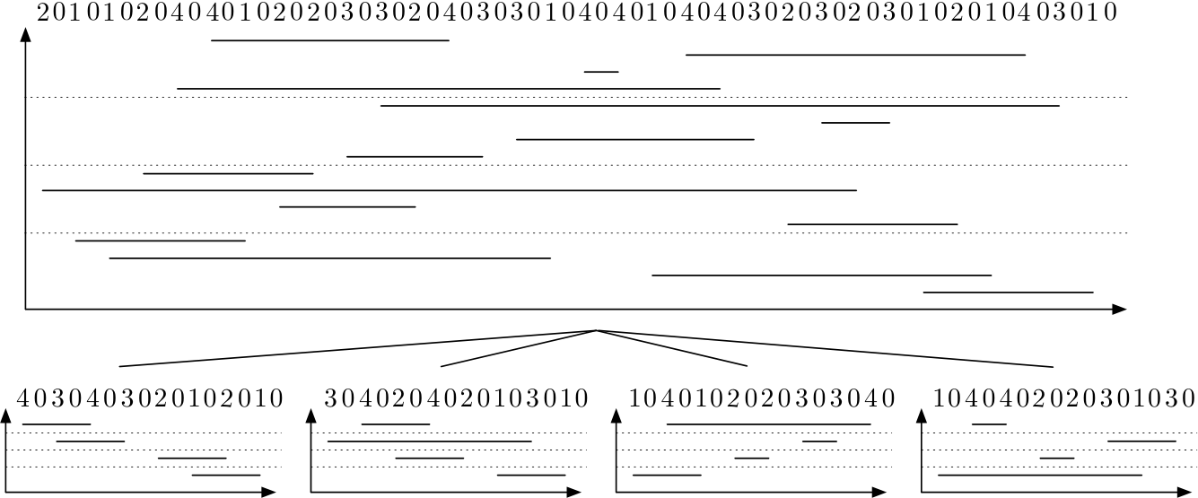
See Figure 3. At node $v$ we use $O(n_{v}\log\log n)$ bits. Since each segment appears in $O(\log n/\log\log n)$ structures the total space is $O(n\frac{\log n}{\log\log n}\log\log n)=O(n\log n)$ bits.

To answer a $\operatorname{\mathsf{segment-select}}(i,j)$ query we perform a top-down search in $R$ starting at the root and ending at the leaf containing the $j$th segment that intersects the vertical line at time $i$. To guide the navigation, we compute local parameters $i_{v}$ and $j_{v}$ at each node $v$, such that $i_{v}$ is the time in $L_{v}$ that corresponds to time $i$ in $E$, and $j_{v}$ is the segment in $L_{v}$ that corresponds to segment $j$ in $L$. At the root $r$, we have $i_{r}=i$ and $j_{r}=j$. Consider an internal node $v$ with children $v_{1},\ldots,v_{\Delta}$ during the traversal. Given the local parameters $i_{v}$ and $j_{v}$ we compute the child to continue the search in and new local parameters. We first compute the slab containing the $j$th segment as

Thus, the search should continue in child $v_{k}$, and we subtract the number of segments in the previous slabs from $j_{v}$ to get $j_{v_{k}}$. To compute $i_{v_{k}}$ we first compute $r_{k}=\operatorname{\mathsf{rank}}(E_{v},i_{v},k)$. Since $i_{v}$ might not be a point in $L_{v_{k}}$ we then set

By Lemma 10 and Lemma 11 each of the above steps takes constant time and hence the total time is $O(\log n/\log\log n)$. We have the following property of $i_{v_{k}}$.

First assume $s\in I_{v}$. Then $x_{1}\leq i_{v}\leq x_{2}$, which implies that $\operatorname{\mathsf{rank}}(E_{v},x_{1},k)\leq\operatorname{\mathsf{rank}}(E_{v},i_{v},k)\leq\operatorname{\mathsf{rank}}(E_{v},x_{2},k)$, that is $r_{1}\leq r_{k}\leq r_{2}$. We need to prove that $x_{1}^{\prime}\leq i_{v_{k}}\leq x_{2}^{\prime}$. If $E_{v}[i_{v}]=k$, i.e., $i_{v}$ is an endpoint of a segment in slab $k$ then it immediately follows that $x_{i}^{\prime}=2r_{1}-1\leq 2r_{k}-1=i_{v_{k}}$ and similarly that $i_{v_{k}}\leq x_{2}^{\prime}$. If $E_{v}[i_{v}]\neq k$ then $i_{v_{k}}$ is not an endpoint in $L_{v_{k}}$ and thus $x_{1}<i_{v}<x_{2}$. This implies that $r_{1}\leq r_{k}<r_{2}$. We have $r_{1}=r_{k}$ in the case where $x_{1}$ is the rightmost endpoint in slab $k$ smaller than $i_{v}$. It follows immediately that $2r_{1}-1\leq 2r_{k}-1<2r_{k}<2r_{2}$, and therefore $x_{1}^{\prime}<i_{v_{k}}<x_{2}^{\prime}$.

Assume $s\in I_{v_{k}}$. Then $x_{1}^{\prime}\leq i_{v_{k}}\leq x_{2}^{\prime}$ and we want to prove that $x_{1}\leq i_{v}\leq x_{2}$. We have $2r_{1}-1\leq i_{v_{k}}\leq 2r_{2}-1$. We will first show that $r_{1}\leq r_{k}\leq r_{2}$. There are two cases. If $E[i_{v}]=k$ then $i_{v_{k}}=2r_{k}-1$ and it follows immediately that $r_{1}\leq r_{k}\leq r_{2}$. If $E[i_{v}]\neq k$ then $i_{v_{k}}=2r_{k}$ and thus $2r_{1}-1\leq i_{v_{k}}\leq 2r_{2}-1$ implies $2r_{1}-1<2r_{k}<2r_{2}-1$ which again implies that $r_{1}\leq r_{k}\leq r_{2}$. By definition of $\operatorname{\mathsf{rank}}$ we have that $\operatorname{\mathsf{rank}}(E_{v},x_{1},k)\leq\operatorname{\mathsf{rank}}(E_{v},i_{v},k)\leq\operatorname{\mathsf{rank}}(E_{v},x_{2},k)$ implies $x_{1}\leq i_{v}\leq x_{2}$. $\blacksquare$

In summary, this proves Theorem 3.

Combined with the reduction in Lemma 8 we obtain a linear space and $O(\log n/\log\log n)$ time solution for the random access problem. To show Theorem 1 it only remains to show how to report a substring of length $\ell$ in $O(\log n/\log\log n+\ell)$ time. To do so we build the hive graph of Chazelle [16] on the segments. This uses $O(n)$ space and allows us to traverse the segments through the vertical line at time $i$ above a given segment in sorted order in constant time per reported segment. To report a substring of length $\ell$ we simply perform the corresponding segment selection and traverse the $\ell$ segments above. By Lemma 7 this gives us the correct substring. This uses $O(\log n/\log\log n+\ell)$ time. This completes the proof of Theorem 1.

Finally, we show how to construct the random access data structure of Theorem 1 in $O(n\log n)$ time. Given a version tree $T$ with $n$ nodes it is straightforward to construct the corresponding instance of the segment selection problem $L$ as described in Section 2 in $O(n)$ time in a single traversal of $T$. We then construct tree $R$ over the segments in $L$ recursively. At each node $v$ we build the slab selection data structure from Section 3 consisting of $n_{v}$ segments. To do so, we construct the grid, the predecessor data structure, and the compact encoding in $O(n_{v})$ time. The global tables for the normalized cells need only be constructed once in $O(n)$ total time. Furthermore, we also need to build the rank/select data structure from Lemma 11. This can also be done in $O(n_{v})$ time, and hence constructing these data structures on all nodes in $R$ takes $O(n\log_{\Delta}n)=O(n\log n/\log\log n)$ time. Finally, constructing the hive graph can be done in $O(n\log n)$ time [16].

We now prove the lower bounds in Theorems 2 and 4 for random access and segment selection, respectively. For the random access problem we show a reduction from the following problem: Let $A$ be an array of $n$ unique integers. The prefix selection problem is to preprocess $A$ to support prefix selection queries, that is, given integers $i$ and $j$ report the $j$th smallest integer in the subarray $A[1..i]$.

Given an input array $A$ to the prefix selection problem, we construct an instance $T$ of the random access problem. Our reduction allows any prefix selection query on $A$ to be answered by a single random access query on $T$. The reduction works even when $T$ is a path without any deletions.

Let $A$ be an array of length $n$ consisting of unique integers in $\{1,\ldots,n\}$. Our instance $T$ is a path of $n+1$ nodes $v_{0},\ldots,v_{n}$ rooted at $v_{0}$. See Figure 4. Edge $(v_{i-1},v_{i})$ is labeled by $\operatorname{\mathsf{insert}}(r_{i},i)$, where $r_{i}$ is the number of entries in $A[1..i]$ that are smaller $A[i]$. We have that $S(v_{i})$ is permutation of indices in $\{1,..,i\}$ corresponding to the sorted order of $A[1..i]$, that is, $A[S(v_{i})[1]]<\cdots<A[S(v_{i})[i]]$. In particular, $S(v_{i})[j]$ is the index of the $j$th smallest integer in $A[1..i]$. Hence, we can answer a prefix selection query $\operatorname{\mathsf{prefix-select}}(i,j)$ by computing $\operatorname{\mathsf{access}}(v_{i},j)$. This completes the proof of Theorem 2.

References

- [1] Pankaj K Agarwal, Lars Arge, Haim Kaplan, Eyal Molad, Robert E Tarjan, and Ke Yi. An optimal dynamic data structure for stabbing-semigroup queries. SIAM J. Comput., 41(1):104–127, 2012.
- [2] Jérémy Barbay, Francisco Claude, Travis Gagie, Gonzalo Navarro, and Yakov Nekrich. Efficient fully-compressed sequence representations. Algorithmica, 69(1):232–268, 2014.
- [3] Jérémy Barbay, Meng He, J Ian Munro, and S Srinivasa Rao. Succinct indexes for strings, binary relations and multi-labeled trees. In Proc. 18th SODA, pages 680–689, 2007.
- [4] Djamal Belazzougui, Patrick Hagge Cording, Simon J. Puglisi, and Yasuo Tabei. Access, rank, and select in grammar-compressed strings. In Proc. 23rd ESA, pages 142–154, 2015.
- [5] Djamal Belazzougui and Gonzalo Navarro. Optimal lower and upper bounds for representing sequences. ACM Trans. Algorithms, 11(4):1–21, 2015.
- [6] Philip Bille, Anders Roy Christiansen, Patrick Hagge Cording, Inge Li Gørtz, Frederik Rye Skjoldjensen, Hjalte Wedel Vildhøj, and Søren Vind. Dynamic relative compression, dynamic partial sums, and substring concatenation. Algorithmica, 80(11):3207–3224, 2018. Announced at ISAAC 2016.
- [7] Philip Bille, Anders Roy Christiansen, Nicola Prezza, and Frederik Rye Skjoldjensen. Succinct partial sums and Fenwick trees. In Proc. 24th SPIRE, pages 91–96, 2017.
- [8] Philip Bille, Mikko Berggren Ettienne, Inge Li Gørtz, and Hjalte Wedel Vildhøj. Time–space trade-offs for lempel–ziv compressed indexing. Theoret. Comput. Sci., 713:66–77, 2018.
- [9] Philip Bille and Inge Li Gørtz. Random access in persistent strings. In Proc. 31st ISAAC, 2020.
- [10] Philip Bille, Inge Li Gørtz, Gad M Landau, and Oren Weimann. Tree compression with top trees. Inform. and Comput., 243:166–177, 2015.
- [11] Philip Bille, Gad M. Landau, Rajeev Raman, Kunihiko Sadakane, Srinivasa Rao Satti, and Oren Weimann. Random access to grammar-compressed strings and trees. SIAM J. Comput., 44(3):513–539, 2015. Announced at SODA 2011.
- [12] Timothy M Chan. Persistent predecessor search and orthogonal point location on the word RAM. ACM Trans. Algorithms, 9(3):1–22, 2013.
- [13] Timothy M Chan and Mihai Pǎtraşcu. Transdichotomous results in computational geometry, i: Point location in sublogarithmic time. SIAM J. Comput., 39(2):703–729, 2009.
- [14] Timothy M Chan and Konstantinos Tsakalidis. Dynamic planar orthogonal point location in sublogarithmic time. In Proc 34th SoCG 2018, 2018.
- [15] M. Charikar, E. Lehman, D. Liu, R. Panigrahy, M. Prabhakaran, A. Sahai, and A. Shelat. The smallest grammar problem. IEEE Trans. Inform. Theory, 51(7):2554–2576, 2005.
- [16] Bernard Chazelle. Filtering search: A new approach to query-answering. SIAM J. Comput., 15(3):703–724, 1986.
- [17] BG Chern, Idoia Ochoa, Alexandros Manolakos, Albert No, Kartik Venkat, and Tsachy Weissman. Reference based genome compression. In Proc. 12th ITW, pages 427–431, 2012.
- [18] Mark De Berg, Marc Vankreveld, and Jack Snoeyink. Two-dimensional and three-dimensional point location in rectangular subdivisions. J. Algorithms, 18(2):256–277, 1995.
- [19] P. F. Dietz. Fully persistent arrays (extended array). In Proceedings of the Workshop on Algorithms and Data Structures, Lecture Notes in Computer Science, volume 382, pages 67–74, 1989.
- [20] Paul F Dietz. Optimal algorithms for list indexing and subset rank. In Proc. 1st WADS, pages 39–46, 1989.
- [21] Huy Hoang Do, Jesper Jansson, Kunihiko Sadakane, and Wing-Kin Sung. Fast relative Lempel–Ziv self-index for similar sequences. Theoret. Comput. Sci., 532:14–30, 2014.
- [22] J. Driscoll, N. Sarnak, D. Sleator, and R. Tarjan. Making data structures persistent. J. Comput. System Sci., 38:86–124, 1989.
- [23] Peter M Fenwick. A new data structure for cumulative frequency tables. Software: Pract. Exper., 24(3):327–336, 1994.
- [24] Paolo Ferragina, Giovanni Manzini, Veli Mäkinen, and Gonzalo Navarro. Compressed representations of sequences and full-text indexes. ACM Trans. Algorithms, 3(2):20, 2007.
- [25] Paolo Ferragina and Rossano Venturini. A simple storage scheme for strings achieving entropy bounds. Theoret. Comput. Sci., 372(1):115 – 121, 2007.
- [26] Michael Fredman and Michael Saks. The cell probe complexity of dynamic data structures. In Proc. 21st STOC, pages 345–354, 1989.
- [27] Michael L. Fredman and Dan E. Willard. Surpassing the information theoretic bound with fusion trees. J. Comput. System Sci., 47(3):424–436, 1993.
- [28] Michael L. Fredman and Dan E. Willard. Trans-dichotomous algorithms for minimum spanning trees and shortest paths. J. Comput. System Sci., 48(3):533–551, 1994.
- [29] Travis Gagie, Paweł Gawrychowski, Juha Kärkkäinen, Yakov Nekrich, and Simon J Puglisi. A faster grammar-based self-index. In Proc. 6th LATA, pages 240–251, 2012.
- [30] Travis Gagie, Paweł Gawrychowski, Juha Kärkkäinen, Yakov Nekrich, and Simon J Puglisi. LZ77-based self-indexing with faster pattern matching. In Proc. 14th LATIN, pages 731–742, 2014.
- [31] Travis Gagie, Paweł Gawrychowski, and Simon J Puglisi. Approximate pattern matching in lz77-compressed texts. J. Discrete Algorithms, 32:64–68, 2015.
- [32] Travis Gagie, Kalle Karhu, Gonzalo Navarro, Simon J Puglisi, and Jouni Sirén. Document listing on repetitive collections. In Proc. 24th CPM, pages 107–119, 2013.
- [33] Moses Ganardi, Artur Jez, and Markus Lohrey. Balancing straight-line programs. In Proc. 60th FOCS, pages 1169–1183, 2019.
- [34] Alexander Golynski, J Ian Munro, and S Srinivasa Rao. Rank/select operations on large alphabets: a tool for text indexing. In Proc. 17th SODA, pages 368–373, 2006.
- [35] Alexander Golynski, Rajeev Raman, and S Srinivasa Rao. On the redundancy of succinct data structures. In Proc. 11th SWAT, pages 148–159, 2008.
- [36] Roberto Grossi, Ankur Gupta, and Jeffrey Scott Vitter. High-order entropy-compressed text indexes. In Proc. 14th SODA, pages 841–850, 2003.
- [37] Roberto Grossi, Rajeev Raman, Satti Srinivasa Rao, and Rossano Venturini. Dynamic compressed strings with random access. In Proc. 40th ICALP, pages 504–515. 2013.
- [38] Wing-Kai Hon, Kunihiko Sadakane, and Wing-Kin Sung. Succinct data structures for searchable partial sums with optimal worst-case performance. Theoret. Comput. Sci., 412(39):5176–5186, 2011.
- [39] Christopher Hoobin, Simon J Puglisi, and Justin Zobel. Relative Lempel-Ziv factorization for efficient storage and retrieval of web collections. Proc. VLDB Endowment, 5(3):265–273, 2011.
- [40] Allan Grønlund Jørgensen and Kasper Green Larsen. Range selection and median: Tight cell probe lower bounds and adaptive data structures. In Proc. 22nd SODA, pages 805–813, 2011.
- [41] Dominik Kempa and Nicola Prezza. At the roots of dictionary compression: String attractors. In Proc. 50th STOC, pages 827–840, 2018.
- [42] Shanika Kuruppu, Simon J Puglisi, and Justin Zobel. Relative Lempel-Ziv compression of genomes for large-scale storage and retrieval. In Proc. 17th SPIRE, pages 201–206, 2010.
- [43] Shanika Kuruppu, Simon J Puglisi, and Justin Zobel. Optimized relative Lempel-Ziv compression of genomes. In Proc. 34th ACSC, pages 91–98, 2011.
- [44] Stan Y. Liao, Srinivas Devadas, and Kurt Keutzer. A text-compression-based method for code size minimization in embedded systems. Trans. Design Autom. Electr. Syst., 4(1):12–38, 1999.
- [45] Stan Y. Liao, Srinivas Devadas, Kurt Keutzer, Steven W. K. Tjiang, and Albert Wang. Code optimization techniques in embedded DSP microprocessors. Design Autom. Emb. Sys., 3(1):59–73, 1998.
- [46] Veli Mäkinen, Gonzalo Navarro, Jouni Sirén, and Niko Välimäki. Storage and retrieval of highly repetitive sequence collections. J. Comput. Biol., 17(3):281–308, 2010.
- [47] J Ian Munro and Yakov Nekrich. Compressed data structures for dynamic sequences. In Proc. 23rd ESA, pages 891–902. 2015.
- [48] Gonzalo Navarro. Indexing highly repetitive collections. In Proc. 23rd IWOCA, pages 274–279, 2012.
- [49] Gonzalo Navarro. Document listing on repetitive collections with guaranteed performance. Theoret. Comput. Sci., 772:58–72, 2019.
- [50] Yakov Nekrich. A dynamic stabbing-max data structure with sub-logarithmic query time. In Proc. 22nd ISAAC, pages 170–179, 2011.
- [51] Mihai Pătraşcu and Mikkel Thorup. Dynamic integer sets with optimal rank, select, and predecessor search. In Proc. 55th FOCS, pages 166–175, 2014.
- [52] Mihai Pǎtraşcu and Erik D. Demaine. Logarithmic lower bounds in the cell-probe model. SIAM J. Comput., 35(4):932–963, 2006. Announced at SODA 2004.
- [53] Rajeev Raman, Venkatesh Raman, and S Srinivasa Rao. Succinct dynamic data structures. In Proc. 7th WADS, pages 426–437, 2001.
- [54] Wojciech Rytter. Application of Lempel-Ziv factorization to the approximation of grammar-based compression. Theoret. Comput. Sci., 302(1-3):211–222, 2003.
- [55] Kunihiko Sadakane and Roberto Grossi. Squeezing succinct data structures into entropy bounds. In Proc. 17th SODA, pages 1230–1239, 2006.
- [56] Neil Sarnak and Robert Endre Tarjan. Planar point location using persistent search trees. Commun. ACM, 29(7):669–679, 1986.
- [57] James A. Storer and Thomas G. Szymanski. The macro model for data compression. In Proc. 10th STOC, pages 30–39, 1978.
- [58] James A Storer and Thomas G Szymanski. Data compression via textual substitution. J. ACM, 29(4):928–951, 1982.
- [59] Robert Endre Tarjan and Uzi Vishkin. Finding biconnected componemts and computing tree functions in logarithmic parallel time. In Proc. 25th FOCS, pages 12–20, 1984.
- [60] Elad Verbin and Wei Yu. Data structure lower bounds on random access to grammar-compressed strings. In Proc. 24th CPM, pages 247–258, 2013.
- [61] Jacob Ziv and Abraham Lempel. A universal algorithm for sequential data compression. IEEE Trans. Inform. Theory, 23(3):337–343, 1977.