Reliable Categorical Variational Inference
with Mixture of Discrete Normalizing Flows
Abstract
Variational approximations are increasingly based on gradient-based optimization of expectations estimated by sampling. Handling discrete latent variables is then challenging because the sampling process is not differentiable. Continuous relaxations, such as the Gumbel-Softmax for categorical distribution, enable gradient-based optimization, but do not define a valid probability mass for discrete observations. In practice, selecting the amount of relaxation is difficult and one needs to optimize an objective that does not align with the desired one, causing problems especially with models having strong meaningful priors. We provide an alternative differentiable reparameterization for categorical distribution by composing it as a mixture of discrete normalizing flows. It defines a proper discrete distribution, allows directly optimizing the evidence lower bound, and is less sensitive to the hyperparameter controlling relaxation.
1 INTRODUCTION
Efficient gradient-based algorithms for variational inference (VI) are nowadays routinely used for model-independent Bayesian inference. VI learns an approximation of some latent variables conditional on observed data . We express the distribution using a differentiable reparameterization , so that it is characterized by a base distribution and a non-linear transformation parameterized by . The parameters are optimized with stochastic gradients of the evidence lower bound (ELBO)
| (1) | ||||
but other variational objectives could also be used.
Handling discrete variables within this framework is challenging as the gradient does not exist. However, most discrete distributions can be expressed in terms of continuous random variables by suitable auxiliary variable augmentation, for example, the binomial and negative binomial distributions using the Polya-Gamma distribution [Polson et al. 2013], and the categorical distribution using the Gumbel distribution [Gumbel 1954]. For categorical distribution this reparameterization is not yet sufficient for gradient-based learning because the required argmax in where , is not differentiable. For learning we hence need to use an approximation replacing the argmax with a continuous relaxation in form of the softmax function. Both Maddison et al. 2017 and Jang et al. 2017 presented simultaneously near-identical treatment of a relaxation scheme (called Gumbel-Softmax (GS) relaxation in this work) for categorical distribution, today routinely used in various learning tasks.
GS relaxation has serious limitations as a variational approximation. It does not define a valid discrete distribution , preventing evaluation of the entropy, and hence one needs to optimize adjusted approximate objectives. Often these objectives do not match well with the true one, and the relaxation is highly sensitive to its hyperparameters with no obvious criteria for selecting them in pure inference tasks. These issues have remained somewhat undisclosed in the literature thanks to highly flexible decoders used in VAEs. However, for models with fixed likelihoods and strong priors GS relaxation is unreliable and burdensome.
We propose a new differentiable parameterization for categorical distributions that builds on discrete normalizing flows (DNF) [Tran et al. 2019]. DNFs model a distribution as flexible transformation of a base distribution, but are not applicable for VI due to dependence on already expressive base distributions. Our newly proposed Mixture of DNFs (MDNF), however, can express any categorical distribution arbitrarily accurately (assuming sufficiently many mixture components) already with delta base distributions (simplistic categorical distributions with all probability mass on one value). MDNF can be trained by gradient optimization, provide discrete samples following the true distribution, and – in contrast to GS relaxation that fallaciously employs continuous probability density – enables estimation of probability mass necessary for calculation of the variational objective. Compared to GS relaxation, MDNF is more reliable for variational approximation since it allows directly optimizing the true objective and does not have hyperparameters that are difficult to select. We demonstrate the first point in Figure 1, and the latter later in Figure 3 (left).
We proceed by first discussing differentiable parameterizations for categorical distributions in general, and then cover their use for variational approximations. Before going to details, we summarize the main contributions: We (a) propose MDNF, new reliable differentiable parameterization for categorical distributions; (b) provide practical learning algorithms for fitting MDNF as variational approximation, including one building on boosting VI [Miller et al. 2017]; (c) show that MDNF is robust to its hyperparameters and provides unbiased estimate of the variational objective (in contrast to GS); (d) show that MDNF outperforms GS relaxation for inference of ordinary graphical models, and is more reliable also for VAEs and (e) introduce partial flows – an extension to discrete flows by Tran et al. 2019 exhibiting better theoretical properties and empirical performance.
2 GRADIENTS OF CATEGORICAL SAMPLES
Without loss of generality, we focus here on a one-dimensional categorical distribution, but in Section 4.2 explain how a set of distributions can be parameterized jointly while avoiding the naive storage cost of . A single categorical distribution is natively parameterized by the probabilities of possible outcomes, with . For the direct parameterization gradients of expectations like (1) are undefined, but next we explain differentiable alternatives: GS relaxation and DNF (both having other limitations).
2.1 Gumbel-Softmax Relaxation
The Gumbel-Softmax (or Concrete) relaxation [Jang et al. 2017, Maddison et al. 2017] consists of three parts: (1) Gumbel augmentation; (2) approximating argmax with softmax; (3) discretizing samples by pushing them through straight-through (ST) operation [Bengio et al. 2013]. The third operation is often omitted since using ’relaxed one-hot’ encodings allows for smoother optimization, though at the cost of needing to adapt the model for continuous samples. We use GS to refer to the latter approach, denoting the discretized one by ST-GS or ST-Gumbel.
The value for the th category of a sample is
The distribution is typically specified via logits for unconstrained optimization, and the temperature hyperparameter controls ‘magnitude’ of gradient so that larger typically makes optimization easier while introducing more bias and for the bias (but also the gradient) disappears.
The (unbounded) density of the GS distribution
| (2) |
is specified for continuous samples , so that for any valid discrete sample (including ) it is . Hence discrete entropy – and variational objective – is not defined (however, see Section 6.1 for discussion on how it can be estimated), and to use GS relaxation for VI one needs to either (a) relax the prior itself using (2) with some arbitrarily chosen temperature or (b) use alternative learning objectives that are not valid bounds for the evidence (but may work in practice). The first choice introduces a second hyperameter and both approaches disconnect the internal learning objective from the desired one (Figure 1). These properties make GS relaxations unreliable for VI.
2.2 Discrete Normalizing Flows
An alternative parameterization for categorical distributions can be built using normalizing flows (NF) [Tabak et al. 2010, Tabak and Turner 2013]. NFs transform some (typically simple) base distribution into the desired one via some invertible transformation with tractable Jacobian retaining the density. With discrete normalizing flows [Tran et al. 2019], the Jacobian is not needed and the probability is simply , but the choice of is considerably more limited – we need an invertible discrete transtormation that can be trained w.r.t. the parameters . Tran et al. 2019 proposed
| (3) |
where denotes a number of possible categories and and need to be coprime. The parameters and are modeled with neural networks with outputs, scaled with a temperature and passed through softmax and the ST operation to obtain discrete one-hot encoded values. That is, we have for a suitable network.
Unfortunately, as also noted by Papamakarios et al. 2019, the expressive power of DNF is seriously limited unless using already powerful base distributions. Since is invertible and the samples and have the same shape, we have one-to-one mapping between and . This implies that the possible values for target probabilities are determined by the values of the base distribution; for each unique with for some , we need for some unique . In other words, DNF can only move probability mass around without changing the values; see Figure 2 for an illustration. For specific constructions there can also be other limitations – for example (3) cannot achieve all permutations – but these can usually be alleviated by stacking multiple flows. Stacking, however, does not help with the more fundamental limitation of inability to change the probability values.
For generative tasks Tran et al. 2019 overcame the problem by first training strong autoregressive or factorized models and showed consistent but somewhat small improvement for DNF fine-tuning the distribution. Training such flexible base distributions is not, however, possible in VI. We are not aware of any attempts of using DNFs for this purpose, even though continuous normalizing flows are frequently used as approximations [Kingma et al. 2016].
3 MIXTURE OF DNF
We present a novel composite parameterization for categorical distributions that combines multiple component distributions using a mixture formulation
| (4) |
where the mixing weights s.t. delegate partial responsibility of the total probability mass to individual component distributions . The set of distributions that can be expressed using (4) naturally depends on and the choice of component distributions, with some obvious special cases: With but arbitrary we retain the direct parameterization, whereas with and we can express any distribution with delta distributions.
We use (4) for representation of arbitrary distributions by using DNFs as flexible and trainable component distributions. The resulting mixture of discrete normalizing flows (MDNF) for parameterization of a categorical distribution defines the probability
| (5) |
where we call component flows. For we get standard DNF, whereas for both sampling and probability evaluation are algorithmically more involved but remain tractable, as described next.
3.1 Operations
Forward sampling for MDNF consists of three stages: (1) choosing a flow , (2) sampling from the base distribution of the th flow (which may be the same for all flows), and (3) passing the sample through the flow to obtain the final sample: . We assume that only the last step is differentiable, and hence the particular sample is a function of associated only with the particular . Direct implementation of this scheme, however, requires a separate dynamic computation graph associated with every sample . For a more efficient implementation using only a single graph, we can mask the outputs, conceptually similar to how masking is used in transformers or masked autoencoders. First, a whole batch consisting of samples is passed through all flows . Then, flow outputs are multiplied with masks responsible for choosing which flow each individual sample is assigned to ( appears exactly for one of the positions). Finally, the masked outputs are summed up using .
Backward evaluation of probability follows the general formulation in (5), i.e., probability of a one-hot encoded sample is obtained by passing the sample through all flows in reverse mode to obtain one-hot encoded samples for which probabilities can be evaluated by using the base distribution associated with the th flow.
3.2 Design
MDNF is compatible with (a) any choice of flows and (b) any base distributions . Next, we discuss practical choices for these.
Flows constructed with (3) are not able to model all possible permutations without stacking multiple transformations and even then we still lack guarantees. Therefore, in Supplement we introduce the alternative of partial flows that allow achieving all permutations by stacking transformations and perform better than (3). However, with the delta base distributions explained below, already one layer of (3) is sufficient, and hence we used it in our experiments.
For ordinary DNFs it is crucial to use expressive base distributions, as explained in Section 2.2, but for MDNF we can use simple base distributions. In fact, already delta distributions that allocate all probability for a single category (that is, ) are sufficient, offering both computational advantage and easy theoretical analysis. Already a single flow of the form (3) (with fixed ) can move the probability to the desired location by shifting with suitable , and with sufficiently large this is enough for modeling arbitrary distributions. Some other base distributions could be more efficient by requiring smaller , but we will show in Section 6 that delta distributions are also a good practical choice.
In more detail, already with uniform weights there exist flows such that the absolute error for any target distribution and any outcome can be bounded by and hence the approximation converges when . This follows directly from approximating each with a subset of the flows, chosen independently so that the proportion of the flows best matches it (see Supplement for details). Note that for single DNF () the bound is trivial, and if allowing for free then is enough for zero error.
4 MDNF FOR VI
We use MDNF for variational approximation of a model with categorical latent variables and observed data . To specify the distribution (for given ), we need to fix the weights and the flows , controlled by the parameters of the network outputting the parameters and .
4.1 Learning Algorithms
The forward sampling of MDNF is differentiable w.r.t , and hence we can optimize the Monte Carlo estimate of a variational objective using reparametrized gradients, e.g., using (1). Below we explain two ways of how it can be done. The first assumes fixed weights, whereas the latter trains individual components one by one in a boosting fashion. Both methods can be generalized for models with also continuous variables, for example, by plugging in also continuous NFs.
VI on Flows (VIF)
The mixture is highly expressive already for fixed . By fixing them to , we can jointly train for all flows with ordinary gradient ascent. One optimization step consists of sampling as explained in Section 3.1 and estimating gradients of the objective following (1), where the Monte Carlo estimate of entropy relies on (5). This algorithm is easy to implement, but simultaneous training of multiple flows is poorly identified - any two flows can be swapped without effect and the mixture has equivalent solutions what may cause problems with direct gradient-based learning.
Boosting VI on Flows (BVIF)
To avoid simultaneous training of competing flows, we turn the attention to existing literature on variational boosting, originally developed for iteratively increasing flexibility of approximations (in context of continuous variables). Variational boosting algorithms construct posterior approximation of the form where we intentionally match notation with (5), so that in our case . We adapt the algorithm of Miller et al. 2017, which proceeds by iteratively training the and by keeping flows and weights up to fixed, using the objective
where denotes a mixture composed from components . The optimization consists of steps, each using a number of gradient ascent iterations. Note, however, that the method can be further extended to automatically find , similar to Giaquinto and Banerjee 2020, for example if combined with a suitable decreasing prior (e.g., stick-breaking process) for the mixing weights .
Boosting Baseline (BVI)
Boosting can, in principle, be used to learn a flexible approximation also without training the individual flows. For completeness, we explain a baseline algorithm doing this, to illustrate the importance of training the individual flows. For fixed component distributions , each of which is a delta distribution (other choices could be used as well), we merely train the weights iteratively as above. This naturally requires large to work well.
4.2 Multivariate Distributions
Until now we have focused on individual 1D categorical distributions, but all the derivations so far are as well valid for multivariate . Multivariate posteriors can be decomposed into 1D distributions as , where each of the distributions is modeled as a DNF with parameters and expressed via neural networks. Those networks model dependencies between the dimensions , typically either using autoregressive or bipartite design. In autoregressive networks, the transformation of the th dimension depends on outputs of the preceding dimensions , i.e., , implemented using a recurrent network such as LSTM [Hochreiter and Schmidhuber 1997] or a masked autoencoder [Germain et al. 2015]. We use the latter. Bipartite networks [Dinh et al. 2015] divide the dimensions into two disjoint sets so that the second set depends only on the outputs for the first set. This simplifies computation (no iterating over is required) but does not allow for modeling arbitrary dependencies (although stacking multiple flows with different subsets helps). Regardless if autoregressive or bipartite, the methods can be used on the level of individual flows or between multiple MDNFs, each being responsible for modeling a 1D distribution. We used the former approach.
Whenever comparing against GS, to be fair, we carry out experiments with factorized approximations . Then, it is sufficient to treat the parameters directly as outputs (logits) of the network, e.g., . Finally, let us also note that arbitrary design of the neural networks and allows to extend their inputs, for example, by including also observed data as or simply , to achieve amortized inference, e.g., with VAEs.
4.3 Bias and Variance
As illustrated in Figure 1, evaluation and monitoring of convergence is difficult for GS relaxations, due to discrepancy between the internal learning objective and the true variational bound. For MDNF, however, the internal learning objective is unbiased estimate of the true objective, and hence can be used for monitoring optimization and convergence, as well as for comparing models. Since (5) defines the probability , similarly as for the joint probability term , we can directly use an unbiased MC estimator also for entropy . This holds for both factorized and non-factorized approximations. For the latter, transforms , where may be (and in our case is) a factorized distribution for which .
The variance of the estimate depends on the number of samples in (1), but is in practice very low. In Supplement we empirically show that even for extreme cases (, large ) the variance is well below 1% of the mean value. We also note that for the VIF algorithm we can reach zero variance with , by deterministically allocating individual samples to component flows in order, instead of sampling .
4.4 Hyperparameters
MDNF has two main hyperparameters, the number of flows and the temperature . We will show in Section 6.2 that selecting is considerably easier than selecting the corresponding pair of and for GS relaxation (Section 2.1). In practice, following Jang et al. 2017, we recommend annealing with for the th iteration, where e.g. and seem to work well in most cases.
Accuracy typically improves roughly monotonically with until saturating. The variational objective is comparable across , and hence we can simply select the best choice after trying a few alternatives; in our case was deemed sufficient. also increases computation time. The detailed complexity depends on type of used and the dimensionality . For example, for an autoregressive flow a forward pass takes and a backward evaluation assuming cost of one dimensional transformation .
5 RELATED WORK
Discrete Latent Variables
Besides the approaches considered here, inference for categorical latent variables can be carried out by specialized model-specific algorithms (e.g., Rolfe 2016, Vahdat et al. 2018 for discrete VAE) or marginalization. For model-independent scenarios an alternative to reparameterization is the REINFORCE algorithm, with recent focus in reducing its variance [Mnih and Gregor 2014, Mnih and Rezende 2016, Tucker et al. 2017]. Besides VI, methods based on relaxation have also been used to enable Hamiltonian dynamics for MCMC [Zhang et al. 2012, Nishimura et al. 2020]. Finally, the quantization-based methods for VAEs by van den Oord et al. 2017, Razavi et al. 2019 can be viewed as kind of relaxation, but with modified objectives. Since they neglect the prior altogether, they do not generalize to general approximations beyond VAE.
Normalizing Flows
Normalizing flows [Van Den Berg et al. 2018, Rezende and Mohamed 2015, Kingma et al. 2016] used for learning flexible posterior approximations and generative distributions for continuous variables have been recently generalized for discrete ordinal [Hoogeboom et al. 2019] and categorical [Tran et al. 2019] variables, but only for generative tasks. Our approach, building on the latter, extends the scope for VI. MDNF resembles also some constructs for continuous normalizing flows, briefly described here even though both the motivation and details differ notably. Papamakarios et al. 2019 proposed a mixture of flows and use an expression similar to (5), but they rely on flows with restricted and non-overlapping (continuous) support in the -space, and hence the mixture actually corresponds to piece-wise application of separate flows. Our approach is also related to the recent mixture formulation, developed independently and in parallel by Giaquinto and Banerjee 2020. Their goal, however, was to improve normalizing flows for posterior inference of continuous models and they did not address discrete latent variables in any way. Similarly, the RAD architecture by Dinh et al. 2019 partitions the domain and uses a mixture model with piecewise invertible maps to learn better continuous distributions. Finally, MDNF shares also certain ideas with Stochastic Normalizing Flows [Hodgkinson et al. 2020] in how sampling consists of a stochastic step (in our case selection of a flow) and a deterministic step with normalizing flows, and with Continuously Indexed Flows [Cornish et al. 2019] in challenging the bijection assumption.
Variational Inference
Compared to the recent alternative of (semi-)implicit approximations that can also be applied for discrete variables [Yin and Zhou 2018, Titsias and Ruiz 2019], MDNF has the advantage of fitting the standard reparameterization framework and that it is directly applicable also with alternative objectives that rely on access to , such as Dieng et al. 2017, Domke and Sheldon 2018. Finally, advances in boosting VI [Locatello et al. 2018a, Guo et al. 2016, Locatello et al. 2018b, Campbell and Li 2019] could be incorporated to improve the BVIF algorithm now based on Miller et al. 2017.
6 EXPERIMENTS
We validate our claims with experiments on Bayesian networks and VAEs that (a) show MDNF is more reliable than GS relaxation, due to unbiased internal objective and easier hyperparameter selection, (b) compare different learning algorithms for MDNF, and (c) verify that delta base distributions are a suitable choice. All details of the experiments (including complete code and data used to produce the results and plots) are provided in Supplement, along with additional experiments on hyperparameters selection, variance of the gradients, partial flows, and a third model (Gaussian mixture model).

6.1 Evaluation
For evaluating the methods we use stochastic estimates for a variational learning objective, in practice ELBO, as well as the KL divergence to the true posterior that can be evaluated for sufficiently small models by exact inference. For MDNF the internal learning objective is unbiased estimate of ELBO, but for GS relaxation this is not the case. Instead, there can be a dramatic discrepancy between the two; Figure 1 compares the internal objective against the estimate described next.
We evaluate the ELBO for GS using empirical estimates obtained for large number of discretized () samples – this is an accurate, but computationally heavy, way of evaluating the approximation. The log-likelihood and log-prior terms of the objective can then be estimated using MC with , but the entropy requires estimating . For factorized posteriors the entropy factorizes as , where each of the factors can be estimated as , and for large asymptotically . Archer et al. 2014 discuss alternative estimators for entropy.
6.2 Reliability of Approximation
Hyperparameters
Using GS for variational approximation requires relaxing both the approximation and the prior [Maddison et al. 2017] and hence GS has two tunable hyperparameters, and , whereas MDNF uses discrete priors and only requires setting . To illustrate the practical difficulty of using GS, we compare MDNF and GS relaxation in ideal conditions where an oracle evaluating the final quality against ground truth is available.
We apply the methods for posterior inference of discrete Bayes networks (BN) with multiple latent nodes (but fixed structure), so that for sufficiently small networks we can evaluate the true posterior by explicit enumeration (with exponential complexity). We use four networks from https://www.bnlearn.com/bnrepository/, so that always 1-2 variables are observed and others are latent, presenting the results for two choices for observed values for each BN. We use Asia (8 binary nodes) Sachs (11 variables with 3 categories), Earthquake (5 binary nodes) and Cancer (5 binary nodes). Optimization details for both MDNF and GS relaxation are provided in Supplement.
Figure 3 (left) illustrates the hyperparameter surfaces for two BNs. For MDNF all temperatures above (we used here fixed temperatures, without annealing) have near identical performance, whereas for both GS variants there is a narrow range of configurations that work well and the optimal choices are different for the two BNs. In summary, selecting good hyperparameters for GS is difficult even when having access to information that could never be available in practice. Note that for MDNF the choice can be based on the internal objective but for GS not – the values across the rows would not be comparable due to different .
Figure 3 (right) shows that even if one was able to select optimal hyperparameters by accessing an oracle, GS relaxation still does not work reliably in this task. The ST variant is uniformly bad, whereas the continuous variant is comparable with MDNF when using the optimal parameters selected specifically for this BN and task (strong oracle). If allowed to access the true posterior but forced to use the same temperature parameters for all BNs and tasks (weak oracle), it already starts performing poorly in many cases. For MDNF there is no notable difference, since constant large is always near optimal.
Internal vs External Objective
We already demonstrated in Figure 1 the difference between the internal objectives and the true quality, carried out with good temperature choices. For example, without ST on Sachs network the variational objective starts growing when internal objective is still clearly improving. The illustrations here are selected examples observed during our experiments, and we note that in some cases the two objectives align a lot better. However, there is no way of identifying when this is the case, which means the method is in general fragile.
6.3 Variational Autoencoder
Gumbel-Softmax relaxation is typically used for training Variational Autoencoders (VAEs) with discrete latent codes, since the flexibility of the decoder can mask issues with the approximation and the choice of temperatures is less critical. We compare MDNF (, VIF algorithm, factorized approximation) against GS in this task. We omit the more computationally demanding BVIF from the experiment (even though it could perform superior to VIF) to avoid an unfair comparison where our method could spend more resources than the baselines.
Besides Gumbel, the only GS method optimizing a valid lower bound, we also compare against three heuristic alternatives often used for VAEs: Jang refers to the objective of Jang et al. 2017 as implemented in https://github.com/ericjang/gumbel-softmax, and Madison Eq. X, refer to two alternatives provided by the corresponding equations in Maddison et al. 2017. For all methods we provide the results with and without ST, use hyperparameters suggested by the authors, and provide optimization details and visual illustrations in Supplement.
Figure 4 presents values of the sample-based variational objective (Section 6.1) for all methods trained on MNIST digits for latent space configurations with increasing total cardinality (number of dimensions times the number of categories ). All methods except ST Gumbel are in general competitive; they work well for at least some configurations. Gumbel is the best for low total cardinality but performs poorly for high cardinality, whereas the opposite holds for Jang and Maddison Eq. 22. MDNF is the only method that works reliably and is close to the best method in all cases. That is, it is consistent and competitive in the tasks GS relaxation is most commonly used.
6.4 Algorithms and Base Distributions
Section 4.1 presented different algorithms for fitting MDNF. Figure 5 (left three subplots) compares them on three BNs, including one larger example of Hepar II (70 nodes with up to 6 categories). BVIF outperforms the baseline of standard DNF (=1) for all three BNs, and increasing improves the result roughly monotonically. For the two smaller networks VIF performs roughly as well, but breaks down for the larger Hepar II network. BVI is clearly inferior, showing that training the component flows is necessary.
Throughout the paper we have used delta base distributions allocating all probability mass for one outcome. To study this choice in practice, we consider an alternative of sampling them from a symmetric Dirichlet . For all realizations are delta distributions and for they are uniform, and by varying we can create base distributions between these extremes. Note that is a worst-case baseline, since re-arranging identical values does not help. For both models very small is optimal (Figure 5 (right)), supporting use of delta distributions.
Supplement replicates the above results for Gaussian mixture models (GMM) on three data sets to illustrate the method can also be used with continuous variables and with more latent variables. MDNF still outperforms DNF, but with marginal gain as the posterior is simpler: for GMMs all probability mass of a data point is often allocated to a single cluster.
7 CONCLUSION
Learning posterior approximations for high-dimensional categorical latent variables is fundamentally more difficult compared to continuous ones. Even though Gumbel Softmax relaxations are widely used for this in the context of VAEs, we showed that they are in practice fragile due to optimization objectives that can be severely biased compared to the true variational objective and because of high sensitivity to hyperparameters. For VAEs these problems are not very severe because using a flexible decoder makes them insensitive to the prior [Zhao et al. 2019], but we demonstrated that even for VAEs our new alternative may be beneficial in terms of reliability (Figure 4). MDNF consistently achieves competitive performance, while being more reliable and easier to tune, offering a practical alternative for future applications.
Our main interest was in posterior inference of proper probabilistic models, such as a discrete Bayes networks, for which Gumbel Softmax is poorly suited. We proposed an alternative reparameterization for categorical distributions – MDNF, that (in practice) does not require fine-tuning of hyperparameters and provides better approximations. Unlike previous approaches, it enables direct probability evaluation and access to the true optimization objective. MDNF builds on discrete normalizing flows, but can express arbitrary categorical distributions without pre-training the base distributions and hence allows plug-and-play use for arbitrary models. We here used MDNF only for variational inference, but it can be used also for generative modeling tasks and has potential for improving on DNF. More generally, even though our work does not directly consider any application domain or task, it helps developing reliable models with discrete structures, which may better match intuition and reality.
Acknowledgements.
This work was supported by the Academy of Finland Flagship program: Finnish Center for Artificial Intelligence, FCAI, and by the Technology Industries Finland and Erkko Foundation: Interactive Artificial Intelligence for Driving R&D.References
- Archer et al. [2014] Evan Archer, Il Memming Park, and Jonathan W Pillow. Bayesian entropy estimation for countable discrete distributions. The Journal of Machine Learning Research, 15(1):2833–2868, 2014.
- Batcher [1968] Kenneth E Batcher. Sorting networks and their applications. In Proceedings of the April 30–May 2, 1968, spring joint computer conference, pages 307–314, 1968.
- Bengio et al. [2013] Yoshua Bengio, Nicholas Léonard, and Aaron Courville. Estimating or propagating gradients through stochastic neurons for conditional computation. arXiv:1308.3432, 2013.
- Bishop [2006] Christopher M Bishop. Pattern recognition and machine learning. Springer, 2006.
- Campbell and Li [2019] Trevor Campbell and Xinglong Li. Universal boosting variational inference. In Advances in Neural Information Processing Systems 32:, pages 3479–3490, 2019.
- Cornish et al. [2019] Rob Cornish, Anthony L. Caterini, George Deligiannidis, and Arnaud Doucet. Relaxing bijectivity constraints with continuously indexed normalising flows. arXiv:1909.13833, 2019.
- Dieng et al. [2017] Adji Bousso Dieng, Dustin Tran, Rajesh Ranganath, John Paisley, and David Blei. Variational inference via chi upper bound minimization. In Advances in Neural Information Processing Systems, pages 2732–2741, 2017.
- Dinh et al. [2015] Laurent Dinh, David Krueger, and Yoshua Bengio. NICE: Non-linear independent components estimation. In 3rd International Conference on Learning Representations, ICLR 2015, Workshop Track Proceedings, 2015.
- Dinh et al. [2019] Laurent Dinh, Jascha Sohl-Dickstein, Razvan Pascanu, and Hugo Larochelle. A RAD approach to deep mixture models. arXiv preprint arXiv:1903.07714, 2019.
- Domke and Sheldon [2018] Justin Domke and Daniel R Sheldon. Importance weighting and variational inference. In Advances in neural information processing systems, pages 4470–4479, 2018.
- Germain et al. [2015] Mathieu Germain, Karol Gregor, Iain Murray, and Hugo Larochelle. MADE: Masked autoencoder for distribution estimation. In International Conference on Machine Learning, pages 881–889, 2015.
- Giaquinto and Banerjee [2020] Robert Giaquinto and Arindam Banerjee. Gradient boosted normalizing flows. Advances in Neural Information Processing Systems, 33, 2020.
- Gumbel [1954] Emil Julius Gumbel. Statistical theory of extreme values and some practical applications: a series of lectures. Technical Report Number 33, US Govt. Print. Office, 1954.
- Guo et al. [2016] Fangjian Guo, Xiangyu Wang, Kai Fan, Tamara Broderick, and David B. Dunson. Boosting variational inference. ArXiv:1611.05559, 2016.
- Hochreiter and Schmidhuber [1997] Sepp Hochreiter and Jürgen Schmidhuber. Long short-term memory. Neural computation, 9(8):1735–1780, 1997.
- Hodgkinson et al. [2020] Liam Hodgkinson, Chris van der Heide, Fred Roosta, and Michael W Mahoney. Stochastic normalizing flows. arXiv preprint arXiv:2002.09547, 2020.
- Hoogeboom et al. [2019] Emiel Hoogeboom, Jorn Peters, Rianne van den Berg, and Max Welling. Integer discrete flows and lossless compression. In Advances in Neural Information Processing Systems, pages 12134–12144, 2019.
- Jang et al. [2017] Eric Jang, Shixiang Gu, and Ben Poole. Categorical reparameterization with Gumbel-Softmax. In International Conference on Learning Representations, 2017.
- Kingma et al. [2016] Durk P Kingma, Tim Salimans, Rafal Jozefowicz, Xi Chen, Ilya Sutskever, and Max Welling. Improved variational inference with inverse autoregressive flow. In Advances in neural information processing systems, pages 4743–4751, 2016.
- Locatello et al. [2018a] Francesco Locatello, Gideon Dresdner, Rajiv Khanna, Isabel Valera, and Gunnar Rätsch. Boosting black box variational inference. In Advances in Neural Information Processing Systems 31, pages 3405–3415, 2018a.
- Locatello et al. [2018b] Francesco Locatello, Rajiv Khanna, Joydeep Ghosh, and Gunnar Rätsch. Boosting variational inference: an optimization perspective. In International Conference on Artificial Intelligence and Statistics, volume 84 of Proceedings of Machine Learning Research, pages 464–472. PMLR, 2018b.
- Maddison et al. [2017] Chris J. Maddison, Andriy Mnih, and Yee Whye Teh. The concrete distribution: A continuous relaxation of discrete random variables. In International Conference on Learning Representations, 2017.
- Miller et al. [2017] Andrew C Miller, Nicholas J Foti, and Ryan P Adams. Variational boosting: Iteratively refining posterior approximations. In International Conference on Machine Learning, pages 2420–2429, 2017.
- Mnih and Gregor [2014] Andriy Mnih and Karol Gregor. Neural variational inference and learning in belief networks. In International Conference on Machine Learning, page II–1791–II–1799, 2014.
- Mnih and Rezende [2016] Andriy Mnih and Danilo J. Rezende. Variational inference for Monte Carlo objectives. In International Conference on Machine Learning, page 2188–2196, 2016.
- Nishimura et al. [2020] Akihiko Nishimura, David B Dunson, and Jianfeng Lu. Discontinuous Hamiltonian Monte Carlo for discrete parameters and discontinuous likelihoods. Biometrika, 107(2):365–380, 2020.
- Papamakarios et al. [2019] George Papamakarios, Eric Nalisnick, Danilo Jimenez Rezende, Shakir Mohamed, and Balaji Lakshminarayanan. Normalizing flows for probabilistic modeling and inference. arXiv:1912.02762, 2019.
- Polson et al. [2013] Nicholas G. Polson, James G. Scott, and Jesse Windle. Bayesian inference for logistic models using Pólya-Gamma latent variables. Journal of the American Statistical Association, 108(504):1339–1349, 2013.
- Razavi et al. [2019] Ali Razavi, Aaron van den Oord, and Oriol Vinyals. Generating diverse high-fidelity images with VQ-VAE-2. In Advances in Neural Information Processing Systems, pages 14837–14847, 2019.
- Renjith et al. [2018] Shini Renjith, A Sreekumar, and M Jathavedan. Evaluation of partitioning clustering algorithms for processing social media data in tourism domain. In 2018 IEEE Recent Advances in Intelligent Computational Systems, pages 127–131. IEEE, 2018.
- Rezende and Mohamed [2015] Danilo Rezende and Shakir Mohamed. Variational inference with normalizing flows. In International Conference on Machine Learning, pages 1530–1538, 2015.
- Rolfe [2016] Jason Tyler Rolfe. Discrete variational autoencoders. In International Conference on Learning Representations, 2016.
- Tabak and Turner [2013] Esteban G Tabak and Cristina V Turner. A family of nonparametric density estimation algorithms. Communications on Pure and Applied Mathematics, 66(2):145–164, 2013.
- Tabak et al. [2010] Esteban G Tabak, Eric Vanden-Eijnden, et al. Density estimation by dual ascent of the log-likelihood. Communications in Mathematical Sciences, 8(1):217–233, 2010.
- Titsias and Ruiz [2019] Michalis K Titsias and Francisco Ruiz. Unbiased implicit variational inference. In The 22nd International Conference on Artificial Intelligence and Statistics, pages 167–176, 2019.
- Tran et al. [2019] Dustin Tran, Keyon Vafa, Kumar Agrawal, Laurent Dinh, and Ben Poole. Discrete flows: Invertible generative models of discrete data. In Advances in Neural Information Processing Systems, pages 14692–14701, 2019.
- Tucker et al. [2017] George Tucker, Andriy Mnih, Chris J Maddison, John Lawson, and Jascha Sohl-Dickstein. Rebar: Low-variance, unbiased gradient estimates for discrete latent variable models. In Advances in Neural Information Processing Systems, pages 2627–2636, 2017.
- Vahdat et al. [2018] Arash Vahdat, William G Macready, Zhengbing Bian, Amir Khoshaman, and Evgeny Andriyash. DVAE++: Discrete variational autoencoders with overlapping transformations. In International Conference on Machine Learning, 2018.
- Van Den Berg et al. [2018] Rianne Van Den Berg, Leonard Hasenclever, Jakub M Tomczak, and Max Welling. Sylvester normalizing flows for variational inference. In 34th Conference on Uncertainty in Artificial Intelligence, pages 393–402, 2018.
- van den Oord et al. [2017] Aaron van den Oord, Oriol Vinyals, and koray kavukcuoglu. Neural discrete representation learning. In Advances in Neural Information Processing Systems 30, pages 6306–6315, 2017.
- Yin and Zhou [2018] Mingzhang Yin and Mingyuan Zhou. Semi-implicit variational inference. In International Conference on Machine Learning, pages 5660–5669, 2018.
- Zhang et al. [2012] Yichuan Zhang, Zoubin Ghahramani, Amos J Storkey, and Charles A. Sutton. Continuous relaxations for discrete Hamiltonian Monte Carlo. In Advances in Neural Information Processing Systems 25, pages 3194–3202, 2012.
- Zhao et al. [2019] Shengjia Zhao, Jiaming Song, and Stefano Ermon. InfoVAE: Balancing learning and inference in variational autoencoders. In AAAI Conference on Artificial Intelligence, volume 33, pages 5885–5892, 2019.
Reliable Categorical Variational Inference
with Mixture of Discrete Normalizing Flows: Supplementary Materials
In the Supplementary Materials, we first provide additional illustrations and details of behavior of MDNF in Section 8, including demonstration of the newly proposed partial flows that are useful also outside variational approximations. Then, in Section 9 we provide both the details of the experimental setup omitted from the main manuscript required for reproducing the experiments, and additional experimental results to complement the ones presented in the main paper.
8 DISCRETE FLOWS AND MIXTURES
Here we illustrate in more detail how the DNF transformation proposed by Tran et al. 2019 works with delta base distributions (Section 8.1), verify the approximation bound in Section 3.2 (Section 8.2), and explain and empirically validate the concept of partial flows (Section 8.3).
8.1 Delta Distributions and Shift Transformations
Even though MDNF can be used with any valid base distributions, delta distributions have two concrete advantages: they do not require complex transformations and are easy to analyse. They allocate all probability mass for one entry, for some , but any delta distribution can be transformed into another one by renaming to some in samples drawn from the distribution. This can be achieved already with a single shift transformation – by a simplified (3) with as
In particular, for any choice of and , we can always find some such that for any delta base distribution using . In practice, we use trainable , and multiple flows in a mixture () to be able to allocate separately (but not independently) fractions of the total probability mass. Figure 6 recreates Figure 1 but for delta base distributions with shift-only transformations.
8.2 Error Bound for Delta Base Distributions
As stated in Section 3.2, for any target distribution over categories, there exist component flows with mixture weights such that
for all . As explained above, a single flow using delta base distribution can allocate all probability mass of that flow for any given category. To verify the bound, it hence remains to show that by combining component flows with uniform weights we can represent any categorical distribution sufficiently accurately. We do this in a constructive manner, and note that the reasoning does not directly say anything about how MDNFs trained with practical learning algorithms would behave.
Let us first assume . We approximate (for each ) using flows, each carrying a probability mass of . Let us first allocate component flows for modeling each category, so that is approximated by . For this it already holds that . However, we have , and hence is not a distribution and there are some unallocated component flows, unless the right inequality is equality (in which case for all ). However, since the number of unallocated flows is at most , we can allocate the remaining ones on arbitrary categories, one for each, so that for these categories. This makes a valid distribution, while retaining the maximum approximation error of .
If we simply set for the smallest probabilities , all of which are guaranteed to be at most , and apply the above procedure to approximate for the remaining categories.
8.3 Partial Flows
MDNF is in principle compatible with any choice of flows . In practice, the location-scale transformation of Tran et al. 2019 in (3) of the main manuscript works fairly well in approximation tasks and is used in the main paper, despite not being able to model all possible transformations without stacking multiple flows (and even then, we still lack guarantees).
For more general uses-cases, we propose an alternative of partial flows that apply the transformation in (3) (usually with ) but only on a subset of positions of a one-hot encoded vector . Instead of acting on vector of length the transformation acts on vector of length . The remaining category positions are passed untouched. Note that the ‘subset’ vectors do need to be valid one-hot encodings anymore and may consist of only in all positions. Such partial flows make, e.g., swapping elements considerably easier; in the extreme case of two elements can be swapped by shifting them by one position, without influencing any of the other probabilities (that would happen when doing the same swap with (3)). By simply stacking partial flows with appropriately chosen subsets of size , we can construct a flow that could perform any reordering (=relabeling) of categories by swapping individual pairs, analogous to bitonic sorter [Batcher 1968]. Partial flows can be implemented with a slight modification of code for ordinary location-scale flows, e.g., by passing only the correct subset for an ordinary discrete flow transformation. Note however that transformation parameters need to receive full vectors when learning dependencies between dimensions.
| Flow | #Layers | #iters | #iters | ||
|---|---|---|---|---|---|
| Loc-scale | 3 | 0.38 | 268 | 0.08 | 1502 |
| 5 | 0.33 | 90 | 0.03 | 886 | |
| 10 | 0.29 | 35 | 0.03 | 376 | |
| 15 | 0.25 | 32 | 0.03 | 595 | |
| 20 | 0.33 | 39 | 0.03 | 687 | |
| 25 | 0.28 | 10 | 0.03 | 163 | |
|
Partial |
10/21 | 1.00 | 78 | 0.78 | 512 |
- fraction of successes
#iters - median of number of iterations
Experimental validation.
To compare partial flows against location-scale flows of (3), we run a controlled experiment with a 1-dimensional variable with categories distributed according to some . We used with categories and with categories. From the distribution , we draw ‘features’ (samples) . Likelihood of the samples is evaluated by passing them in a reverse direction () through a stack consisting of a number of either partial of location-scale flows to get samples for which base probabilities are known. For partial flows we always used and organized them in a way resembling a bubble-sort sorting network (Figure 7) so we used 10 flows for and 21 flows for . For location-scale flows we experimented with stacks of 3-25 identical layers. In each of the repeated runs, we created a new base distribution by randomly shuffling and optimized the stacked flows to maximize the likelihood by using Adam optimizer with learning rate 0.1 and . The optimal solution is reached only when categories of are correctly reordered back, so that samples , follow . This happens only for one of permutations.
Table 1 presents results estimated with repeated runs, where as a success we count only the perfect recovery of the original probability distribution within at most iterations. Partial flows are superior with both and categories, but require more iterations for convergence. Additionally, for stacked location-scale flows, we observe that increasing the number of layers makes learning harder, i.e., the success is achieved in fewer cases (but also in fewer iterations).
9 EXPERIMENTS
In this section, we provide additional details of the main experiments presented in Section 6, including specification of models and networks used for transformations in MDNF. For most experiments we also present additional result figures and tables. Furthermore, we extend the experiment of Section 6.4 for another model family, namely mixture of Gaussians.
In all of the experiments, we used delta base distributions, and therefore it was sufficient to use single-layer flows with shift-only transformation. The shifts we found using standard gradient-based optimizers (RMSprop and Adam). In all cases, following the common practice for Gumbel Softmax relaxations (see for example, Jang et al. 2017), we also performed annealing of the temperature hyperparameter controlling bias of gradients of the straight-through estimator, by slowly decreasing its value in each iteration with , where controls the rate of annealing. An exception to this rule are the experiments on hyperparameter sensitivity, where we used constant temperatures to streamline the experiment and the presentation of the results. We replicated those experiments with annealing but decided not to duplicate the result plots as the results are highly similar and all of the main conclusions hold also when using annealing.
| Sachs [akt=L] | Sachs [akt=H] | Asia [asia=y] | Asia [asia=y, xray=y] | Earthquake [marycalls=T] | Earthquake [marycalls=F] | Cancer [cancer=T] | Cancer [cancer=F] | ||
|---|---|---|---|---|---|---|---|---|---|
| weak | ST Gumbel | 3.70 | 9.30 | 6.51 | 9.75 | 2.55 | 6.07 | 2.64 | 0.68 |
| Gumbel | 2.76 | 8.18 | 0.59 | 4.30 | 0.83 | 0.07 | 1.38 | 1.03 | |
| MDNF | 1.90 | 0.68 | 1.29 | 0.15 | 0.86 | 0.01 | 0.03 | 0.01 | |
| strong | ST Gumbel | 2.49 | 8.11 | 6.51 | 4.15 | 0.80 | 0.05 | 0.87 | 0.11 |
| Gumbel | 0.97 | 1.70 | 0.55 | 2.41 | 0.81 | 0.02 | 0.35 | 0.00 | |
| MDNF | 1.90 | 0.68 | 1.24 | 0.13 | 0.86 | 0.01 | 0.02 | 0.01 |
9.1 Reliability of Approximation (Complements Section 6.2)
Details
For this experiment we used factorized posteriors with constant temperature for both MDNF and GS. MDNFs were trained with VIF and the flows’ shifts were represented directly as . Monte-carlo estimate (with samples) of ELBO we optimized w.r.t. the parameters of a MDNF using RMSprop with learning rate , until convergence or for up to 10000 iterations. In this experiment we used constant temperatures for all methods, simply to make the experiment easier to read. For completeness, we also repeated the experiment with temperature annealing. For MDNF annealing always helps, whereas for GS the behavior is inconsistent – it may as well deteriorate results, but the differences are not significant.
Additional Results
Table 2 presents the numerical results for the graphical summary presented in Figure 3 (right) of the main manuscript. For each of the four Bayesian networks, we fixed one or two of the variables to two alternative observed values (indicated in the table) and considered all other variables as unobserved.
Figure 8 extends the hyperparameter selection illustrations in Figure 3 (left), by providing the corresponding plots for all eight cases, replicating also the two cases provided in the main paper for ease of comparison. The main observations hold in all cases: Selecting the temperature for MDNF is always easy, whereas for Gumbel Softmax the surface is more complicated.

9.2 Variational Autoencoders (Complements Section 6.3)
Gumbel

ST Gumbel Softmax

MDNF (our)
Details
For the VAE experiment we used MDNF as illustrated in Figure 9. The encoder’s output is passed to each of the component flows and parameterizes the flows’ transformation (the transformations factorize over latent dimensions ). For the base distributions we used delta distributions, making it sufficient to use a single shift transformation with each of the used flows.
The encoder and decoder architectures match the ones used by Jang et al. 201711 1 https://github.com/ericjang/gumbel-softmax. The encoder has two dense layers with 512 and 256 nodes and ReLU activations, outputting (for variables of categories each) logits . The decoder has the same layers in reverse order, taking inputs of size and outputting 768 logits for Bernoulli distributions for the pixels. The flow transformations are obtained by passing the encoder’s output through a network with a hidden layer consisting of nodes with ReLU activations and outputting tensors of the same shape.
Our implementation of training follows closely the one by Jang et al. 20171: We used Adam with learning rate , minibatches of size and uniform priors , that for some of the Gumbel Softmax variants needed to be relaxed with . For MDNF we used , for GS we kept , and the annealing was set to . Training of the VAE-MDNF we performed with VIF.
Additional Results
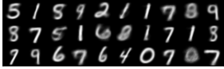
To complement the numerical comparison in Figure 4, we present examples of digits sampled from the models for one of the latent variable configurations in Figure 10. We here illustrate the samples generated from MDNF and the primary competing method of Gumbel Softmax with relaxed priors; the samples for other variants are also very similar.
9.3 Algorithms and Base Distributions (Complements Section 6.4)
Details
In this experiment we used four small-to-medium sized publicly available22 2 https://www.bnlearn.com/bnrepository/ networks for which the true posterior can be evaluated by direct enumeration (apart from Hepar), observing values for 1-2 variables and leaving all others latent. We used Asia (8 binary nodes; we fix asia:=yes and xray:=yes), Sachs (11 variables with 3 categories; we fix Akt:=LOW) and Hepar II (70 nodes with up to 6 categories; we fix carcinoma:=present). To approximate the posteriors, we used masked autoencoders [Germain et al. 2015] (MADE) representing flows’ shifts as , where we set the initial temperature and annealing rate . Monte-carlo estimate (with samples) of ELBO we optimized w.r.t. the parameters of a MDNF using RMSprop with learning rate .
The Asia and Sachs have the same cardinality for all variables, but for Hepar II the cardinality depends on the variable and ranges from 2 to 6. To handle the varying dimensionality in an environment designed for processing fixed-size tensors (in our case TensorFlow), to represent -dimensional samples, we use tensors of size with , and map excess positions in one-hot encoded vectors (category positions with numbers larger than ) down to positions representing valid categories (by summing up zeros and ones from respective positions) only at the end – when evaluating joint probability of observed and latent variables for a model. Entropy term can not be handled this way, but entropy for variables with categories bounds the entropy for the original set of variables, , and with Hepar II we used the approximation.
Additional Results
To complement the analysis of BNs, we replicated the whole experiment on another model family. In particular, we provide an example of a model with both discrete and continuous latent variables, a Gaussian mixture model (GMM) [Bishop 2006]. GMM allocates observed data points to one of clusters with latent -dimensional categorical variables (one per data point; the assignments are assumed to be conditionally independent). Note that we here denote – somewhat unconventionally – by the number of samples to emphasize that in our context the modeling task concerns learning the -dimensional distribution of the latent allocations.
The model with multivariate normal component distributions is
with priors
where we used , , , , and .
The model was trained using closed form Variational EM [Bishop 2006] by alternating updates of the allocations (E-step) and the cluster parameters (M-step). Our implementation and choice of the hyperparameters follow a publicly available implementation33 3 \smallerhttps://github.com/ctgk/PRML/blob/master/prml/rv/variational_gaussian_mixture.py, where we replaced the closed-form E-step with stochastic gradient-based optimization of ELBO w.r.t. parameters of a MDNF modeling the distribution of latent allocations . The optimization we performed using RMSprop optimizer (learning rate ) with samples used for MC estimate of the objective. The posterior for factorizes and therefore we also used factorized flows with . That is, we passed the trainable parameters directly through softmax and the straight-through (ST) operation. In variational EM with gradient-based E-step, stochastic optimization is performed multiple times, each time for slightly different clusters’ found in M-step. The temperature annealing was adapted to this so that we anneal slightly in each step and then in each iteration of the step, e.g., in our schedule with initial temperature and rate .
Figure 11 compares BVIF and VIF for three data sets: 2-dimensional simulated data with 3 partially overlapping clusters (100 points each) with centers in (0,2),(1.7,-1),(-1.7,-1) and diagonal unit covariances; and for Google44 4 https://archive.ics.uci.edu/ml/datasets/Tarvel+Review+Ratings (5456 data points with 24 features) and TripAdivsor55 5 https://archive.ics.uci.edu/ml/datasets/Travel+Reviews (980 points with 10 features) travel reviews [Renjith et al. 2018]. In all our experiments we used – the same number of clusters that was used to generate the simulated data, and that was suggested for the Google set by the authors [Renjith et al. 2018] who provided the data. They also indicated is good, though not necessarily optimal, for TripAdivsor. We dropped BVI that performed very poorly for BNs, and again demonstrate that MDNF works as intended and sometimes improves on top of DNF (B=1), but for these simpler posteriors the difference is marginal because in non-overlapping case all probability mass of a data point posterior is allocated to a single cluster. Nevertheless, we see that MDNF can be used as plug-and-play approximation and works even when modeling a relatively large number of variables.
Finally, Figure 12 presents additional illustrations regarding the choice of the base distribution and temperature hyperparameters, for both BNs and GMMs. We already showed in Figure 5 (right) how delta distributions are ideal for BNs (repeated for convenience here; top left), and here we show that this is the case also for GMMs (top right). In addition, we show that the main result of MDNF being robust for the temperature choice (Section 6.2) holds also in these experiments (bottom row); for both models and optimization algorithms large is good and there is no need to fine-tune the hyperparameter.
9.4 Variance of the MDNF-based ELBO Estimator (Complements Section 4.3)
In Section 4.3 we stated that the variance of the variational objective estimate for MDNF is small. Figure 13 verifies this empirically for a VAE model as used in Section 6.3. We ran VIF with MDNF (B=40) for one full epoch, and then we sample the ELBO 100 times (always using only sample) and evaluate the empirical mean and variance of the estimate; the plot reports the variation as standard deviation normalized by the mean value. For all considered latent variable cardinalities, the deviation is less than 0.35% (ratio of ) of the mean estimate, despite using only a single sample to estimate the objective.