跳到论文正文
W Papers独立论文阅读器 arXiv:2006.15513 论文正文 计算阅读时间 · 0%
引用这篇论文根据当前论文元数据生成,正式投稿前建议核对。


License: arXiv.org perpetual non-exclusive license
arXiv:2006.15513v2 [hep-ph] 13 Sep 2020

Probing new physics effects in 𝚲b→𝚲(→pπ−)ℓ+ℓ−\Lambda_{b}\to\Lambda(\to p\pi^{-})\ell^{+}\ell^{-} decay via model independent approach
Aqsa Nasrullah1, 11 1 aqsanasrullah54@gmail.com, Ishtiaq Ahmed2, M. Jamil Aslam1, Z. Asghar3,4, Saba Shafaq5
 1Department of Physics, Quaid-i-Azam University, Islamabad 45320, Pakistan.
2National Centre for Physics, Quaid-i-Azam University, Islamabad 45320, Pakistan.
3 Center for Mathematical Sciences, Pakistan Institute of Engineering and Applied Sciences, Nilore, Islamabad 45650, Pakistan
4 Department of Physics and applied sciences, Pakistan Institute of Engineering and Applied Sciences, Nilore, Islamabad 45650, Pakistan
5 Department of Physics, International Islamic University, Islamabad 44000, Pakistan.

Abstract

The New Physics (NP) effects are studied in the rare baryonic decay Λb→Λ(→pπ−)ℓ+ℓ−\Lambda_{b}\to\Lambda(\to p\pi^{-})\ell^{+}\ell^{-}, with unpolarized Λb\Lambda_{b} using most general model independent approach by introducing new axial(vector), (pseudo)scalar and tensor operators in the weak effective Hamiltonian corresponding to b→sb\to s transitions. Recently, for Λb→Λ(→pπ−)μ+μ−\Lambda_{b}\to\Lambda(\to p\pi^{-})\mu^{+}\mu^{-} decay the LHCb collaboration has measured the branching ratio (d​ℬ/d​s)(d\mathcal{B}/ds), lepton- and hadron-side forward-backward asymmetries, denoted by AF​BℓA_{FB}^{\ell} and AF​BΛA_{FB}^{\Lambda}, respectively, and the longitudinal polarization fraction FLF_{L} both in the low- and high-recoil regions. To see whether the new V​AVA, S​PSP and TT couplings can accommodate the available experimental data of these observables, first we have examined their influence on these observables and later we have checked the imprints of these new couplings on a number of interesting but yet not measured observables; namely the combined lepton-hadron forward-backward asymmetry (AF​Bℓ​Λ)(A_{FB}^{\ell\Lambda}), transverse polarization fraction (FT)(F_{T}), asymmetry parameters αi′​s\alpha_{i}^{\prime}s and some other angular observables, extracted from certain foldings. It is found that compared to the V​AVA the S​PSP couplings favor experimental data for all the four observables but still no individual coupling is able to accommodate all of the available data simultaneously. To achieve this goal, the pairs of new WCs are taken to check their range that simultaneously satisfy constraints of BB-Physics and available LHCb data on d​ℬ/d​sd\mathcal{B}/ds, FLF_{L}, AF​BℓA_{FB}^{\ell} and AF​BΛA_{FB}^{\Lambda} in several bins for the decay channel under consideration. We find that most of the available data could be accommodated by the different pairs of V​AVA and S​PSP WCs giving more severe constraints on the parametric space of these WCs that is still satisfied with the BB-physics data.

1 Introduction

The rare exclusive B→K∗,ϕ⁡(ρ)​ℓ+​ℓ−B\to K^{*},\phi(\rho)\ell^{+}\ell^{-} decays, governed by the quark level transitions b→s⁡(d)​γb\rightarrow s(d)\gamma or b→s⁡(d)​ℓ+​ℓ−b\rightarrow s(d)\ell^{+}\ell^{-}, have been the focus of the theoretical and experimental studies for some time. The prime reason for them to be at the spotlight is due to their potential to test the predictions of Standard Model (SM) for different observables such as branching fractions, angular distributions and the lepton flavor universality. Though the interest in such decays dates back to the era of B-factories, the recent triggering point was the measurements at the LHCb, most prominently the P5′P_{5}^{\prime} anomaly DescotesGenon:2012zf; Descotes-Genon:2013vna in B→K∗​μ+​μ−B\rightarrow K^{*}\mu^{+}\mu^{-} decay Aaij:2013qta; Aaij:2015oid. Later, the interest in these rare decays was enhanced when the deviations from the SM predictions were observed in the measurements of the lepton flavor universality RKR_{K} and RK∗R_{K^{*}}(RK(∗)=d​ℬ/d​s​(B→K(∗)​μ+​μ−)/d​ℬ/d​s​(B→K(∗)​e+​e−)R_{K^{(*)}}=d\mathcal{B}/ds(B\rightarrow K^{(*)}\mu^{+}\mu^{-})/d\mathcal{B}/ds(B\rightarrow K^{(*)}e^{+}e^{-})) Aaij:2014ora; Bordone:2016gaq; Aaij:2017vbb. Similarly, the deviations are also observed in the differential decay rate of Bs→ϕ​μ+​μ−B_{s}\rightarrow\phi\mu^{+}\mu^{-} Aaij:2013aln; Horgan:2013pva; Aaij:2015esa, the branching ratios of B→D∗​τ​νB\rightarrow D^{*}\tau\nu Fajfer:2012vx and B→K(∗)​μ+​μ−B\rightarrow K^{(*)}\mu^{+}\mu^{-} Aaij:2014pli. Moreover, the BaBar Collaboration measured the lepton flavor universality violation Huschle:2015rga; Aaij:2017uff in RDR_{D} and RD∗R_{D^{*}} (RD(∗)=d​ℬ/d​s​(B→D(∗)​τ​ντ)/d​ℬ/d​s​(B→D(∗)​ℓ​νℓ)R_{D^{(*)}}=d\mathcal{B}/ds(B\rightarrow D^{(*)}\tau\nu_{\tau})/d\mathcal{B}/ds(B\rightarrow D^{(*)}\ell\nu_{\ell}) where ℓ=e,μ\ell=e,\mu). These mismatch between the SM predictions and experimental measurements are rather significant (2​σ−3.4​σ2\sigma-3.4\sigma) Lees:2012xj, providing clear hints of the presence of some new couplings along with that of the SM ones. Due to these facts, the four-body decay B→K∗(→Kπ)ℓ+ℓ−B\rightarrow K^{*}(\to K\pi)\ell^{+}\ell^{-} has been extensively studied in literature Kruger:1997jk; Aliev:1999gp; Aliev:1999re; Kruger:2005ep; Altmannshofer:2008dz; Becirevic:2011bp; Bobeth:2010wg; Faessler:2002ut; Matias:2012qz; Mahmoudi:2014mja. More precise experimental studies are already part of the programs for the LHC upgrade LHCb-19 and Belle-II Belle-II, and there is no doubt that these decays will help us to to see if these anomalies are due to physics beyond the SM or it involve some QCD physics. Supposing that these anomalies persist in future data, similar kind of deviations would also expected to be seen in the baryonic partners of these rare B−B-meson decays, especially in Λb→Λ(→pπ−)ℓ+ℓ−\Lambda_{b}\to\Lambda\left(\to p\pi^{-}\right)\ell^{+}\ell^{-} decays.

The advantage of the baryon decay Λb→Λ(→pπ−)ℓ+ℓ−\Lambda_{b}\to\Lambda\left(\to p\pi^{-}\right)\ell^{+}\ell^{-} over B→K∗(→Kπ)ℓ+ℓ−B\rightarrow K^{*}(\to K\pi)\ell^{+}\ell^{-} is that even the initial state baryons Λb\Lambda_{b} are unpolarized, the final state baryon Λ\Lambda spin can be used to understand the helicity structure of weak effective Hamiltonian Mannel:1997xy; Hiller:2007ur; Wang:2008sm; Chen:2001ki; Faessler:2002ut; Gutsche:2013pp; Gutsche:2013oea. Furthermore, similar to the B→K∗(→Kπ)ℓ+ℓ−B\rightarrow K^{*}(\to K\pi)\ell^{+}\ell^{-} decay, it also provides a large number of angular observables and is sensitive to all the Dirac structures present in the weak Hamiltonian. As the number of angular observables increases due to the polarization of Λb\Lambda_{b} baryon, it makes this decay to be more prolific to test new physics (NP) Bhattacharya:2019der. Due to these distinctive features, the radiative and semileptonic Λb\Lambda_{b} decays have been well studied in the literature Korner:1994nh; Huang:1998ek; Hiller:2001zj; Mott:2011cx; Gutsche:2013pp; Gutsche:2013oea; Detmold:2016pkz; Roy:2017dum; Das:2018iap. To look for the imprints of NP in Λb\Lambda_{b} decays, there are some dedicated studies of this decay in different NP models, namely in 2HDM Aliev:1999ap, Z′Z^{\prime} model Nasrullah:2018puc, Randall-Sundrum model with custodial protection Nasrullah:2018vky, Left-right models Chen:2001zc, Supersymmetric theories Aslam:2008hp and using a most general model independent weak effective Hamiltonian Aliev:2002ww; Aliev:2002tr. In model independent approach the study of Λb→Λ​ℓ+​ℓ−\Lambda_{b}\rightarrow\Lambda\ell^{+}\ell^{-} decay is confined to the analysis of branching ratio (d​ℬ/d​sd\mathcal{B}/ds) and lepton-side forward-backward asymmetry (AF​BℓA_{FB}^{\ell}). However, an analysis of full set of angular observables for this decay have already in other approaches, see e.g., Chen:2001zc; Nasrullah:2018puc; Hu:2017qxj showing that these are quite sensitive to the parameters of different NP models. Motivated by these studies, the present work focuses the analysis of Λb→Λ​ℓ+​ℓ−\Lambda_{b}\rightarrow\Lambda\ell^{+}\ell^{-} decay in the model independent approach. Particularly, we study the Λb→Λ(→pπ)ℓ+ℓ−\Lambda_{b}\rightarrow\Lambda(\to p\pi)\ell^{+}\ell^{-} decay, with unpolarized Λb\Lambda_{b}, using a most general effective Hamiltonian involving new (axial)vector (V​A)(VA) with combination V+AV+A, pseudo(scalar) (S​P)(SP) and the tensor (T)(T) operators. Being an exclusive decay process, some of the physical observables are not clean due to the uncertainties arsing from the form factors (FF). However, some high level precision lattice QCD calculations of FFs are available for Λb→Λ\Lambda_{b}\to\Lambda Detmold:2016pkz transition and by using the Bourrely-Caprini-Lellouch parametrization their profile in the full momentum transfer square (q2=s)(q^{2}=s) is obtained in Bourrely:2008za. The lattice results are not only consistent with the recent QCD light- cone sum rule calculations Wang:2015ndk but also have much smaller uncertainty in most of the kinematic range.

It is a well established fact that in contrast to the BB-decays, the QCD factorization is not fully developed for the bb-baryon decays, therefore, we will not include the non-factorizable contributions in the present study. It is also important to emphasis that a similar study is performed for the few observables, namely, d​ℬ/d​sd\mathcal{B}/ds, AF​BℓA_{FB}^{\ell} and FLF_{L} in ref. Das:2018sms. However, in comparison to this the present study is quite extensive, especially in two ways: the first and the most important is that we have taken the four-folded decay rate distribution which helps us to explore some more interesting physical observables which depend both on the angle of cascade decay θΛ\theta_{\Lambda} and on the angle ϕ\phi. The second is to see the lepton mass effects on the observables, we keep the terms involving the mass of the final state lepton which are previously ignored in Das:2018sms and hence helping us to extend our analysis to the case when we have τ\tau’s in the final state. As a first step, by using the constraints on the NP Wilson coefficients (WCs) given in Das:2018sms, we reproduced their results of d​ℬ/d​sd\mathcal{B}/ds, AF​BℓA_{FB}^{\ell} and FLF_{L} in Λb→Λ(→pπ)μ+μ−\Lambda_{b}\rightarrow\Lambda(\to p\pi)\mu^{+}\mu^{-} decay. Later, we see the imprints of these new operators on the longitudinal asymmetry αL\alpha_{L}, the transverse asymmetry αU\alpha_{U} and the observables named as 𝒫i′\mathcal{P}_{i}^{\prime}’s that are derived from different foldings and hence have minimal dependence on the form factor. We have already mentioned that non-factorizable contributions which are quite challenging to calculate in Λb→Λ​ℓ+​ℓ−\Lambda_{b}\to\Lambda\ell^{+}\ell^{-} decay might question the analysis of different observables in the large-recoil region; i.e., for dilepton invariant masses s<mJ/ψ2s<m^{2}_{J/\psi}, therefore, to see the imprints of NP we have discussed these observables separately in the low-recoil bin too.

The study performed here is organized as follows: Sect. 2 discusses the effective Hamiltonian of the SM and its extension to take care of the NP operators arising due to the model independent approach. In the same section, the matrix elements of Λb→Λ\Lambda_{b}\to\Lambda for different possible currents are expressed in terms of the FFs. Also, a brief discussion on the formalism of cascade decay Λ→p​π−\Lambda\rightarrow p\pi^{-} is given at the end of this section. The four folded angular distribution and the expressions of physical observables for different NP operators are given in Sect. 3. The discussion of the impact of new V​AVA, S​PSP and TT couplings on different physical observables has been done in section 4, where we also discuss the lepton mass effects in Λb→Λ(→pπ)ℓ+ℓ−\Lambda_{b}\rightarrow\Lambda(\to p\pi)\ell^{+}\ell^{-} decay. In the same section, we present the simultaneous plots of observables for which experimental data is available to see if we could find the values of the pairs of NP WCs that can satisfy the experimental data for more than one physical observables. At the end of Sect. 4, impact of lepton mass effects on different observables is briefly explored for Λ(→pπ)τ+τ−\Lambda(\to p\pi)\tau^{+}\tau^{-}. Finally, the main findings of this study are concluded in Sect. 5. At the end, the Appendix provides the details of the calculation of different helicity fractions for hadron and leptons for all possible operators.

2 Effective Hamiltonian

In the SM the exclusive Λb​(PΛb)→Λ⁡(PΛ)​ℓ+​(q1)​ℓ−​(q2)\Lambda_{b}(P_{\Lambda_{b}})\rightarrow\Lambda(P_{\Lambda})\ell^{+}(q_{1})\ell^{-}(q_{2}) decay is governed by the the four fermion operators build out of V−AV-A currents for the quark level b→sb\to s transitions and the vector/axial vector leptonic currents. In the most general model independent approach extend the operator basis to new (pseudo)scalar and tensor operators, and the V+AV+A combination for the b→sb\to s transitions. The relevant Hamiltonian in this case is Das:2018sms:

ℋe​f​f\displaystyle\mathcal{H}_{eff} =\displaystyle= −GF​αe2​πVt​bVt​s∗[(C9e​f​fs¯γμPLb−2​mbsC7e​f​fs¯iqνσμ​νPRb+CVs¯γμPLb+CV′s¯γμPRb)ℓ¯γμℓ\displaystyle-\frac{G_{F}\alpha_{e}}{\sqrt{2}\pi}V_{tb}V_{ts}^{*}\bigg[\left(C_{9}^{eff}\bar{s}\gamma^{\mu}P_{L}b-\frac{2m_{b}}{s}C_{7}^{eff}\bar{s}iq_{\nu}\sigma^{\mu\nu}P_{R}b+C_{V}\bar{s}\gamma^{\mu}P_{L}b+C_{V}^{\prime}\bar{s}\gamma^{\mu}P_{R}b\right)\bar{\ell}\gamma_{\mu}\ell (1)
+(C10​s¯​γμ​PL​b+CA​s¯​γμ​PL​b+CA′​s¯​γμ​PR​b)​ℓ¯​γμ​γ5​ℓ+(CS′​s¯​PL​b+CS​P¯R​b)​ℓ¯​ℓ\displaystyle+\left(C_{10}\bar{s}\gamma^{\mu}P_{L}b+C_{A}\bar{s}\gamma^{\mu}P_{L}b+C_{A}^{\prime}\bar{s}\gamma^{\mu}P_{R}b\right)\bar{\ell}\gamma_{\mu}\gamma_{5}\ell+\left(C_{S}^{\prime}\bar{s}P_{L}b+C_{S}\bar{P}_{R}b\right)\bar{\ell}\ell
+(CP′s¯PLb+CPs¯PRb)ℓ¯γ5ℓ+CT(s¯σμ​νb)ℓ¯σμ​νℓ+CT5(s¯σμ​νb)ℓ¯σμ​νγ5ℓ]\displaystyle+\left(C_{P}^{\prime}\bar{s}P_{L}b+C_{P}\bar{s}P_{R}b\right)\bar{\ell}\gamma_{5}\ell+C_{T}\left(\bar{s}\sigma^{\mu\nu}b\right)\bar{\ell}\sigma_{\mu\nu}\ell+C_{T_{5}}\left(\bar{s}\sigma^{\mu\nu}b\right)\bar{\ell}\sigma_{\mu\nu}\gamma_{5}\ell\bigg]

where GFG_{F} is Fermi-constant, αe\alpha_{e} is fine structure constant, Vt​b​Vt​s∗V_{tb}V_{ts}^{*} are the corresponding elements of CKM matrix, s≡q2s\equiv q^{2} is dilepton mass squared Faessler:2002ut; Gutsche:2013pp; Gutsche:2013oea and PR,L=1±γ52P_{R,L}=\frac{1\pm\gamma_{5}}{2}. In SM, the WCs C(′)V,C(′)A,C(′)S,C(′)P,CTC^{(\prime)}_{V},\;C^{(\prime)}_{A},\;C^{(\prime)}_{S},\;C^{(\prime)}_{P},\;C_{T}\; and CT5C_{T_{5}} are equal to zero and the explicit form of the SM WCs C7,9e​f​fC_{7,9}^{eff} that has been used in this study are given in Nasrullah:2018vky.

Collecting the vector and axial-vector operators from Eq. (1), the relevant V​AVA part of the Hamiltonian is

ℋV​A=−GF​αe2​π​Vt​b​Vt​s∗​[(HVμ​C~9+−HAμ​C~9−−2​mbs​C7e​f​f​(HTμ+HT5μ))​ℓ¯​γμ​ℓ+(HVμ​C~10+−HAμ​C~10−)​ℓ¯​γμ​γ5​ℓ].\mathcal{H}_{VA}=-\frac{G_{F}\alpha_{e}}{\sqrt{2}\pi}V_{tb}V_{ts}^{*}\bigg[\left(H_{V}^{\mu}\widetilde{C}_{9}^{+}-H_{A}^{\mu}\widetilde{C}_{9}^{-}-\frac{2m_{b}}{s}C_{7}^{eff}(H_{T}^{\mu}+H_{T_{5}}^{\mu})\right)\bar{\ell}\gamma_{\mu}\ell+\left(H_{V}^{\mu}\widetilde{C}_{10}^{+}-H_{A}^{\mu}\widetilde{C}_{10}^{-}\right)\bar{\ell}\gamma_{\mu}\gamma_{5}\ell\bigg]. (2)

where HVμ=12​(s¯​γμ​b)H_{V}^{\mu}=\frac{1}{2}\left(\bar{s}\gamma^{\mu}b\right) and HAμ=12​(s¯​γμ​γ5​b)H_{A}^{\mu}=\frac{1}{2}\left(\bar{s}\gamma^{\mu}\gamma_{5}b\right) with C~9+=C9e​f​f+CV+CV′\widetilde{C}_{9}^{+}=C_{9}^{eff}+C_{V}+C_{V}^{\prime}, C~9−=C9e​f​f+CV−CV′\widetilde{C}_{9}^{-}=C_{9}^{eff}+C_{V}-C_{V}^{\prime}, C~10+=C10e​f​f+CA+CA′\widetilde{C}_{10}^{+}=C_{10}^{eff}+C_{A}+C_{A}^{\prime} and C~10−=C10e​f​f+CA−CA′\widetilde{C}_{10}^{-}=C_{10}^{eff}+C_{A}-C_{A}^{\prime}.

Writing CS,P±=CS,P±CS,P′C_{S,P}^{\pm}=C_{S,P}\pm C_{S,P}^{\prime}, the scalar-pseudoscalar (S​P)(SP) part of weak effective Hamiltonian is

ℋS​P=[CS+​HS+CS−​HP]​ℓ¯​ℓ+[CP+​HS+CP−​HP]​ℓ¯​γ5​ℓ\mathcal{H}_{SP}=[C_{S}^{+}H_{S}+C_{S}^{-}H_{P}]\overline{\ell}\ell+[C_{P}^{+}H_{S}+C_{P}^{-}H_{P}]\overline{\ell}\gamma_{5}\ell (3)

with HS=s¯​bH_{S}=\bar{s}b and HP=s¯​γ5​bH_{P}=\bar{s}\gamma_{5}b. Likewise, we can write the tensor (T)(T) part from Eq. (1) as

ℋT′=−GF​αe2​π​Vt​b​Vt​s∗​[(s¯​σμ​ν​b)​ℓ¯​σμ​ν​(CT+CT5​γ5)​ℓ].\mathcal{H}_{T^{\prime}}=-\frac{G_{F}\alpha_{e}}{\sqrt{2}\pi}V_{tb}V_{ts}^{*}\bigg[\left(\bar{s}\sigma^{\mu\nu}b\right)\bar{\ell}\sigma_{\mu\nu}\left(C_{T}+C_{T_{5}}\gamma_{5}\right)\ell\bigg]. (4)

2.1 Matrix Elements

As an exclusive process, the matrix elements for Λb→Λ\Lambda_{b}\to\Lambda transition for different possible currents can be parameterized in terms of FFs, ft,0,⟂V,ft,0,⟂A,f0,⟂Tf^{V}_{t,0,\perp},\;f^{A}_{t,0,\perp},\;f^{T}_{0,\perp} and f0,⟂T5f^{T_{5}}_{0,\perp} Feldmann:2011xf. In case of vector-currents the corresponding matrix elements for Λb→Λ\Lambda_{b}\to\Lambda become

⟨Λ⁡(PΛ,sΛ)​|s¯​γμ​b|​Λb​(PΛb,sΛb)⟩\displaystyle\langle\Lambda\left(P_{\Lambda},\;s_{\Lambda}\right)\left|\bar{s}\gamma^{\mu}b\right|\Lambda_{b}\left(P_{\Lambda_{b}},\;s_{\Lambda_{b}}\right)\rangle =\displaystyle= u¯(PΛb,sΛb)[ftV(s)(mΛb−mΛ)qμs+f0V(s)mΛb+mΛs+\displaystyle\bar{u}\left(P_{\Lambda_{b}},\;s_{\Lambda_{b}}\right)\bigg[f^{V}_{t}\left(s\right)\left(m_{\Lambda_{b}}-m_{\Lambda}\right)\frac{q^{\mu}}{s}+f_{0}^{V}\left(s\right)\frac{m_{\Lambda_{b}}+m_{\Lambda}}{s_{+}} (5)
×(PΛbμ+PΛμ−qμs​(mΛb2−mΛ2))\displaystyle\times\left(P^{\mu}_{\Lambda_{b}}+P^{\mu}_{\Lambda}-\frac{q^{\mu}}{s}\left(m^{2}_{\Lambda_{b}}-m^{2}_{\Lambda}\right)\right)
+f⟂V(s)(γμ−2​mΛs+PΛbμ−2​mΛbs+PΛμ)]u(PΛ,sΛ),\displaystyle+f_{\perp}^{V}\left(s\right)\left(\gamma^{\mu}-\frac{2m_{\Lambda}}{s_{+}}P^{\mu}_{\Lambda_{b}}-\frac{2m_{\Lambda_{b}}}{s_{+}}P^{\mu}_{\Lambda}\right)\bigg]u\left(P_{\Lambda},\;s_{\Lambda}\right),

with s+=(mΛb+mΛ)2−ss_{+}=(m_{\Lambda_{b}}+m_{\Lambda})^{2}-s and q=PΛb−PΛq=P_{\Lambda_{b}}-P_{\Lambda}. Similarly, by sandwiching the axial-vector currents between Λb\Lambda_{b} and Λ\Lambda, the corresponding matrix elements can be written as

⟨Λ⁡(PΛ,sΛ)​|s¯​γμ​γ5​b|​Λb​(PΛb,sΛb)⟩\displaystyle\langle\Lambda\left(P_{\Lambda},\;s_{\Lambda}\right)\left|\bar{s}\gamma^{\mu}\gamma_{5}b\right|\Lambda_{b}\left(P_{\Lambda_{b}},\;s_{\Lambda_{b}}\right)\rangle =\displaystyle= −u¯(PΛb,sΛb)[ftA(s)(mΛb+mΛ)qμs+f0A(s)mΛb−mΛs−\displaystyle-\bar{u}\left(P_{\Lambda_{b}},\;s_{\Lambda_{b}}\right)\bigg[f^{A}_{t}\left(s\right)\left(m_{\Lambda_{b}}+m_{\Lambda}\right)\frac{q^{\mu}}{s}+f_{0}^{A}\left(s\right)\frac{m_{\Lambda_{b}}-m_{\Lambda}}{s_{-}} (6)
×(PΛbμ+PΛμ−qμs​(mΛb2−mΛ2))\displaystyle\times\left(P^{\mu}_{\Lambda_{b}}+P^{\mu}_{\Lambda}-\frac{q^{\mu}}{s}\left(m^{2}_{\Lambda_{b}}-m^{2}_{\Lambda}\right)\right)
+f⟂V(s)(γμ+2​mΛs+PΛbμ−2​mΛbs−PΛμ)]u(PΛ,sΛ).\displaystyle+f_{\perp}^{V}\left(s\right)\left(\gamma^{\mu}+\frac{2m_{\Lambda}}{s_{+}}P^{\mu}_{\Lambda_{b}}-\frac{2m_{\Lambda_{b}}}{s_{-}}P^{\mu}_{\Lambda}\right)\bigg]u\left(P_{\Lambda},\;s_{\Lambda}\right).

For the dipole operators i​s¯​qν​σμ​ν​bi\bar{s}q_{\nu}\sigma^{\mu\nu}b and i​s¯​qν​σμ​ν​γ5​bi\bar{s}q_{\nu}\sigma^{\mu\nu}\gamma_{5}b, the respective transition matrix elements are

⟨Λ⁡(PΛ,sΛ)​|s¯​i​σμ​ν​qν​b|​Λb​(PΛb,sΛb)⟩\displaystyle\langle\Lambda\left(P_{\Lambda},\;s_{\Lambda}\right)\left|\bar{s}i\sigma^{\mu\nu}q_{\nu}b\right|\Lambda_{b}\left(P_{\Lambda_{b}},\;s_{\Lambda_{b}}\right)\rangle =\displaystyle= −u¯(PΛb,sΛb)[f0Tss+(PΛbμ+PΛμ−qμs(mΛb2−mΛ2))\displaystyle-\bar{u}\left(P_{\Lambda_{b}},\;s_{\Lambda_{b}}\right)\bigg[f_{0}^{T}\frac{s}{s_{+}}\left(P^{\mu}_{\Lambda_{b}}+P^{\mu}_{\Lambda}-\frac{q^{\mu}}{s}\left(m^{2}_{\Lambda_{b}}-m^{2}_{\Lambda}\right)\right) (7)
+f⟂T(mΛb+mΛ)(γμ−2​mΛs+PΛbμ−2​mΛbs+PΛμ)]u(PΛ,sΛ),\displaystyle+f_{\perp}^{T}\left(m_{\Lambda_{b}}+m_{\Lambda}\right)\left(\gamma^{\mu}-\frac{2m_{\Lambda}}{s_{+}}P^{\mu}_{\Lambda_{b}}-\frac{2m_{\Lambda_{b}}}{s_{+}}P^{\mu}_{\Lambda}\right)\bigg]u\left(P_{\Lambda},\;s_{\Lambda}\right),

and

⟨Λ⁡(PΛ,sΛ)​|s¯​i​σμ​ν​qν​γ5​b|​Λb​(PΛb,sΛb)⟩\displaystyle\langle\Lambda\left(P_{\Lambda},\;s_{\Lambda}\right)\left|\bar{s}i\sigma^{\mu\nu}q_{\nu}\gamma_{5}b\right|\Lambda_{b}\left(P_{\Lambda_{b}},\;s_{\Lambda_{b}}\right)\rangle =\displaystyle= −u¯(PΛb,sΛb)γ5[f0T5ss−(PΛbμ+PΛμ−qμs(mΛb2−mΛ2))\displaystyle-\bar{u}\left(P_{\Lambda_{b}},\;s_{\Lambda_{b}}\right)\gamma_{5}\bigg[f_{0}^{T_{5}}\frac{s}{s_{-}}\left(P^{\mu}_{\Lambda_{b}}+P^{\mu}_{\Lambda}-\frac{q^{\mu}}{s}\left(m^{2}_{\Lambda_{b}}-m^{2}_{\Lambda}\right)\right) (8)
+f⟂T5(mΛb−mΛ)(γμ+2​mΛs−PΛbμ−2​mΛbs−PΛμ)]u(PΛ,sΛ).\displaystyle+f_{\perp}^{T_{5}}\left(m_{\Lambda_{b}}-m_{\Lambda}\right)\left(\gamma^{\mu}+\frac{2m_{\Lambda}}{s_{-}}P^{\mu}_{\Lambda_{b}}-\frac{2m_{\Lambda_{b}}}{s_{-}}P^{\mu}_{\Lambda}\right)\bigg]u\left(P_{\Lambda},\;s_{\Lambda}\right).

The matrix elements for the scalar and pseudo-scalar currents can be obtained from Eq. (5) and Eq. (6) after contracting with the di-lepton momentum transfer qμq_{\mu} and invoking the Dirac equation. This gives

⟨Λ⁡(PΛ,sΛ)​|s¯​b|​Λb​(PΛb,sΛb)⟩\displaystyle\langle\Lambda\left(P_{\Lambda},\;s_{\Lambda}\right)\left|\bar{s}b\right|\Lambda_{b}\left(P_{\Lambda_{b}},\;s_{\Lambda_{b}}\right)\rangle =\displaystyle= ftV​(s)​mΛb−mΛmb​u¯​(PΛb,sΛb)​u​(PΛ,sΛ)\displaystyle f^{V}_{t}\left(s\right)\frac{m_{\Lambda_{b}}-m_{\Lambda}}{m_{b}}\bar{u}\left(P_{\Lambda_{b}},\;s_{\Lambda_{b}}\right)u\left(P_{\Lambda},\;s_{\Lambda}\right) (9)
⟨Λ⁡(PΛ,sΛ)​|s¯​γ5​b|​Λb​(PΛb,sΛb)⟩\displaystyle\langle\Lambda\left(P_{\Lambda},\;s_{\Lambda}\right)\left|\bar{s}\gamma_{5}b\right|\Lambda_{b}\left(P_{\Lambda_{b}},\;s_{\Lambda_{b}}\right)\rangle =\displaystyle= ftA​(s)​mΛb+mΛmb​u¯​(PΛb,sΛb)​γ5​u​(PΛ,sΛ).\displaystyle f^{A}_{t}\left(s\right)\frac{m_{\Lambda_{b}}+m_{\Lambda}}{m_{b}}\bar{u}\left(P_{\Lambda_{b}},\;s_{\Lambda_{b}}\right)\gamma_{5}u\left(P_{\Lambda},\;s_{\Lambda}\right). (10)

where we have ignored the strange quark mass. One can see from above equation that these currents do not contribute any new FFs.

In the theoretical study of the exclusive decays, FFs being the non-perturbative quantities are the major source of uncertainties and hence having a good control on their precise calculation is always a need of time. To address this, several approaches have been opted to compute them, e.g., the quark models Cheng:1995fe; Mohanta:1999id; Mott:2011cx, the Lattice QCD Detmold:2016pkz, light cone sum rules (LCSR) Aliev:2010uy; Khodjamirian:2011jp and the perturbative QCD approach He:2006ud. In order to reduce the number of independent FFs, some effective theories are used, e.g., the Heavy quark effective theory (HQET) Hussain:1990uu; Hussain:1992rb helps to reduce the number of independent FFs from ten to two i.e., the Isuger-wise relations ξ1\xi_{1} and ξ2\xi_{2}. Similarly, in soft-collinear effective theory (SCET) the evaluation of the FFs Feldmann:2011xf reduces this number to one. In our analysis, we use the FFs calculated by using Lattice QCD for full dilepton mass square range and these can be expressed as Detmold:2016pkz:

f⁡(s)=a0f+a1f​z​(s)1−s/(mp​o​l​ef)2f(s)=\frac{a^{f}_{0}+a^{f}_{1}z(s)}{1-s/(m^{f}_{pole})^{2}} (11)

The inputs a0fa^{f}_{0} and a1fa^{f}_{1} are given in table V and mp​o​l​efm^{f}_{pole} in Table III of Detmold:2016pkz and these are summarized in Tables I and II of Nasrullah:2018puc with the replacement of f0,+,⟂V→ft, 0,⟂Vf^{V}_{0,\;+,\;\perp}\to f^{V}_{t,\;0,\;\perp}, g0,+,⟂→ft, 0,⟂Ag_{0,\;+,\;\perp}\to f^{A}_{t,\;0,\;\perp}, h+,⟂→f0,⟂Th_{+,\;\perp}\to f^{T}_{0,\;\perp} and h+,⟂→f0,⟂T5h_{+,\;\perp}\to f^{T_{5}}_{0,\;\perp}. The parameter zz is defined as Detmold:2016pkz

z⁡(s)=t+−s−t+−t0t+−s+t+−t0,z(s)=\frac{\sqrt{t_{+}-s}-\sqrt{t_{+}-t_{0}}}{\sqrt{t_{+}-s}+\sqrt{t_{+}-t_{0}}}, (12)

where t0=(mΛb−mΛ)2t_{0}=(m_{\Lambda_{b}}-m_{\Lambda})^{2} and t+=(mB−mK)2t_{+}=(m_{B}-m_{K})^{2}.

2.2 Cascade Decay Λ→p​π−\Lambda\rightarrow p\pi^{-}

The SM effective Hamiltonian for the cascade decay Λ→p​π\Lambda\rightarrow p\pi is given as

HΛe​f​f=4​GF2​Vu​s​Vu​d∗​(d¯​γμ​PL​u)​(u¯​γμ​PL​s).\displaystyle H_{\Lambda}^{eff}=\frac{4G_{F}}{\sqrt{2}}V_{us}V_{ud}^{*}(\bar{d}\gamma^{\mu}P_{L}u)(\bar{u}\gamma^{\mu}P_{L}s). (13)

Again, by using the Hamiltonian (13) between initial state Λ\Lambda and final state pp, the matrix elements can be expressed in term of the QCD parameters (see ref. Boer:2014kda for details). The non-zero helicity contributions to the total decay width for this decay are

Γ′(+1/2,+1/2)\displaystyle\Gamma^{\prime}(+1/2,+1/2) =\displaystyle= (1+αcosθΛ)ΓΛΓ′(+1/2,−1/2)=−αsinθΛei​ϕΓΛ\displaystyle(1+\alpha\cos{\theta_{\Lambda}})\Gamma_{\Lambda}\hskip 56.9055pt\Gamma^{\prime}(+1/2,-1/2)=-\alpha\sin{\theta_{\Lambda}}e^{i\phi}\Gamma_{\Lambda}
Γ′(−1/2,−1/2)\displaystyle\Gamma^{\prime}(-1/2,-1/2) =\displaystyle= (1−αcosθΛ)ΓΛΓ′(−1/2,+1/2)=−αsinθΛe−i​ϕΓΛ\displaystyle(1-\alpha\cos{\theta_{\Lambda}})\Gamma_{\Lambda}\hskip 56.9055pt\Gamma^{\prime}(-1/2,+1/2)=-\alpha\sin{\theta_{\Lambda}}e^{-i\phi}\Gamma_{\Lambda} (14)

where ΓΛ\Gamma_{\Lambda} is the decay width of Λ→p​π\Lambda\to p\pi.

3 Four Fold Angular Distribution and Physical Observables

The four fold differential decay width for the four-body decay process Λb→Λ(→pπ)ℓ+ℓ−\Lambda_{b}\rightarrow\Lambda(\rightarrow p\pi)\ell^{+}\ell^{-} is

d4​ΓdsdcosθℓdcosθΛdϕ=d​ΓV​A+d​ΓS​P+d​ΓT′+d​ΓV​A−S​P+d​ΓV​A−T′+d​ΓS​P−T′,\displaystyle\frac{d^{4}\Gamma}{ds\;d\cos{\theta_{\ell}}d\cos{\theta_{\Lambda}}d\phi}=d\Gamma_{VA}+d\Gamma_{SP}+d\Gamma_{T^{\prime}}+d\Gamma_{VA-SP}+d\Gamma_{VA-T^{\prime}}+d\Gamma_{SP-T^{\prime}},

denoting

d​Γi=d4​ΓidsdcosθℓdcosθΛdϕ\displaystyle d\Gamma_{i}=\frac{d^{4}\Gamma_{i}}{dsd\cos{\theta_{\ell}}d\cos{\theta_{\Lambda}}d\phi}

with i=V​A,S​P,T′,V​A−S​P,V​A−T′i=VA,\;SP,\;T^{\prime},\;VA-SP,\;VA-T^{\prime} and S​P−T′SP-T^{\prime}. Eq. (3) can be written in the form of different matrix elements as

d4​ΓdsdcosθℓdcosθΛdϕ=𝒩[|MV​A|2+|MS​P|2+|MT′|2+(MV​AMS​P∗+MV​AMT′∗+MS​PMT′∗+h.c.)],\displaystyle\frac{d^{4}\Gamma}{dsd\cos{\theta_{\ell}}d\cos{\theta_{\Lambda}}d\phi}=\mathcal{N}\left[|M_{VA}|^{2}+|M_{SP}|^{2}+|M_{T^{\prime}}|^{2}+\left(M_{VA}M^{*}_{SP}+M_{VA}M^{*}_{T^{\prime}}+M_{SP}M^{*}_{T^{\prime}}+h.c.\right)\right], (15)

where the normalization constant 𝒩\mathcal{N} is given by

𝒩=(GF​αe​Vt​b​Vt​s∗)2​λ​v3×211​mΛb3​π5,\displaystyle\mathcal{N}=\frac{(G_{F}\alpha_{e}V_{tb}V_{ts}^{*})^{2}\lambda v}{3\times 2^{11}m_{\Lambda_{b}}^{3}\pi^{5}},

with v=1−4​mℓ2sv=\sqrt{1-\frac{4m_{\ell}^{2}}{s}} and λ=(mΛb2−mΛ2−s)2+4​s​mΛ2\lambda=(m_{\Lambda_{b}}^{2}-m_{\Lambda}^{2}-s)^{2}+4sm_{\Lambda}^{2}. The non-zero helicity components of hadron and lepton current are given in the Appendix. Here, we would like to mention that our expressions of the lepton helicity components corresponding to different currents include the lepton mass term and by setting it equal to zero, these are reduced to the simple ones given in Das:2018sms.

As in the SM, the currents corresponding to Λb→Λ​ℓ+​ℓ−\Lambda_{b}\to\Lambda\ell^{+}\ell^{-} is vector and axial-vector with combination V−AV-A, therefore, the contribution of V​AVA operators will only modify some of the angular coefficients appearing in the SM. However, contributions from the scalar and pseudo-scalar operators which are absent in the SM will introduce the new angular coefficients. Putting everything together the four-fold angular decay distribution for Λb→Λ(→pπ)ℓ+ℓ−\Lambda_{b}\to\Lambda(\to p\pi)\ell^{+}\ell^{-} becomes

d4​ΓdsdcosθℓdcosθΛdϕ\displaystyle\frac{d^{4}\Gamma}{ds\ d\cos{\theta}_{\ell}\ d\cos{\theta_{\Lambda}}\ d\phi} =\displaystyle= 38​π[K1​s​ssin2θℓ+K1​c​ccos2θℓ+K1​ccosθℓ+(K2​s​ssin2θℓ+K2​c​ccos2θℓ+K2​ccosθℓ)cosθΛ\displaystyle\frac{3}{8\pi}\bigg[K_{1ss}\sin^{2}{\theta_{\ell}}+K_{1cc}\cos^{2}{\theta_{\ell}}+K_{1c}\cos{\theta_{\ell}}+(K_{2ss}\sin^{2}{\theta_{\ell}}+K_{2cc}\cos^{2}{\theta_{\ell}}+K_{2c}\cos{\theta_{\ell}})\cos{\theta_{\Lambda}} (16)
+((K3​s​ccosθℓ+K3​s)sinθℓ)sinθΛsinϕ+((K4​s​ccosθℓ+K4​s)sinθℓ)sinθΛcosϕ].\displaystyle+\left((K_{3sc}\cos{\theta_{\ell}}+K_{3s})\sin{\theta_{\ell}}\right)\sin{\theta_{\Lambda}}\sin{\phi}+((K_{4sc}\cos{\theta_{\ell}}+K_{4s})\sin{\theta_{\ell}})\sin{\theta_{\Lambda}}\cos{\phi}\bigg].

In order to extract the different angular observables, we will follow the approach adopted in Refs. Nasrullah:2018puc and Hu:2017qxj, the explicit expressions of the physical observables of interest in our model independent approach are

d​Γd​s\displaystyle\frac{d\Gamma}{ds} =\displaystyle= K1​s​s+K1​c​c,AF​Bℓ=3​K1​c4​K1​s​s+2​K1​c​c,AF​BΛ=2​K2​s​s+K2​c​c4​K1​s​s+2​K1​c​c,\displaystyle K_{1ss}+K_{1cc},\hskip 42.67912ptA_{FB}^{\ell}=\frac{3K_{1c}}{4K_{1ss}+2K_{1cc}},\hskip 42.67912ptA_{FB}^{\Lambda}=\frac{2K_{2ss}+K_{2cc}}{4K_{1ss}+2K_{1cc}},
AF​Bℓ​Λ\displaystyle A_{FB}^{\ell\Lambda} =\displaystyle= 3​K2​c8​K1​s​s+4​K1​c​c,αU=K~2​c​cK1​c​c,αL=K~2​s​sK1​s​s,\displaystyle\frac{3K_{2c}}{8K_{1ss}+4K_{1cc}},\hskip 42.67912pt\alpha_{U}=\frac{\widetilde{K}_{2cc}}{K_{1cc}},\hskip 93.89418pt\alpha_{L}=\frac{\widetilde{K}_{2ss}}{K_{1ss}},\hskip 68.28644pt
αθΛ\displaystyle\alpha_{\theta_{\Lambda}} =\displaystyle= K~2​c​c+2​K~2​s​sK1​c​c+2​K1​s​s,αθℓ=K1​c​c−K1​s​sK1​s​s,αθℓ′=K1​cK1​s​s,\displaystyle\frac{\widetilde{K}_{2cc}+2\widetilde{K}_{2ss}}{{K}_{1cc}+2{K}_{1ss}},\hskip 45.52458pt\alpha_{\theta_{\ell}}=\frac{K_{1cc}-K_{1ss}}{K_{1ss}},\hskip 59.75095pt\alpha^{\prime}_{\theta_{\ell}}=\frac{{K}_{1c}}{K_{1ss}},
αϕ\displaystyle\alpha_{\phi} =\displaystyle= 3​π2​K~4​s16​(K1​c​c+2​K1​s​s),αϕ′=3​π2​K~3​s16​(K1​c​c+2​K1​s​s),𝒫3=2​K2​cΓ^,\displaystyle\frac{3\pi^{2}\widetilde{K}_{4s}}{16(K_{1cc}+2K_{1ss})},\hskip 31.2982pt\alpha^{\prime}_{\phi}=\frac{3\pi^{2}\widetilde{K}_{3s}}{16(K_{1cc}+2K_{1ss})},\hskip 39.83368pt\mathcal{P}_{3}=\frac{2K_{2c}}{\widehat{\Gamma}},
𝒫8\displaystyle\mathcal{P}_{8} =\displaystyle= 4​K1​cΓ^,𝒫9=4​K2​c​cΓ^,Y2=3​(K2​c​c−K2​s​s)8​Γ^,\displaystyle\frac{4K_{1c}}{\widehat{\Gamma}},\hskip 85.35826pt\mathcal{P}_{9}=\frac{4K_{2cc}}{\widehat{\Gamma}},\hskip 91.04872ptY_{2}=\frac{3(K_{2cc}-K_{2ss})}{8\widehat{\Gamma}},
Y3​s​c\displaystyle Y_{3sc} =\displaystyle= K3​s​c2​Γ^,Y4​s​c=K4​s​c2​Γ^,\displaystyle\frac{K_{3sc}}{2\widehat{\Gamma}},\hskip 85.35826ptY_{4sc}=\frac{K_{4sc}}{2\widehat{\Gamma}}, (17)

where K~i,j=Ki,jαΛ\widetilde{K}_{i,j}=\frac{K_{i,j}}{\alpha_{\Lambda}} and Γ^=d​Γd​s\widehat{\Gamma}=\frac{d\Gamma}{ds}. The detailed expressions of Ki,jK_{i,j} in terms of helicity amplitudes are given in the Appendix. In Eq. (17), αΛ\alpha_{\Lambda} is the asymmetry parameter corresponding to the parity violating Λ→p​π−\Lambda\to p\pi^{-} decay and its experimentally measured value is 0.642±0.0130.642\pm 0.013 Patrignani:2016xqp.

4 Impact of New Couplings on Physical Observables

In this section, we will discuss the impact of the NP couplings corresponding to V​AVA, S​PSP and TT operators on the different physical observables discussed above. First we start with d​ℬ/d​sd\mathcal{B}/ds, FLF_{L}, AF​BℓA_{FB}^{\ell} and AF​BΛA_{FB}^{\Lambda} for which the experimental data is available. By using the most recent constraints on NP couplings from Altmannshofer:2017fio, the idea behind this approach is to see whether these NP couplings accommodate the currently available data Aaij:2015xza or not. To accomplish this task, first of all we discuss the impact of individual NP couplings on the above mentioned observables and later we analyze their simultaneous impact. In doing so, we will explore all the available range of new couplings constrained by B−B-meson decays in different bins of ss. After this, we will discuss the observables Y2, 3​s​c, 4​s​cY_{2,\;3sc,\;4sc}, 𝒫3, 8, 9\mathcal{P}_{3,\;8,\;9} and α(′)i\alpha^{(\prime)}_{i} where, i=θℓ,θΛ,ξ,L,Ui=\theta_{\ell},\;\theta_{\Lambda},\;\xi,\;L,\;U which show minimum dependence on the FFs and hence are the potential candidates to search for NP in some on going and future experiments. In order to present our results of different physical observables, we plot them against the square of the momentum transfer ss in the SM as well as in the presence of NP couplings. In these plots, we have presented our results both for the zero and non-zero lepton (μ\mu) mass. Therefore, our formalism is more general from the previous study of the same decay presented in ref. Das:2018sms. Just to distinguish the lepton mass effects Gutsche:2015mxa, we have also discussed the different physical observables for Λb→Λ(→pπ)τ+τ−\Lambda_{b}\to\Lambda(\to p\pi)\tau^{+}\tau^{-} decay where the mass of final state τ′\tau^{\prime}s is significantly large compared to the μ′​s\mu^{\prime}s case. Here, we would like to emphasis that all the plots are drawn for the central values of the FFs however, in order to quantify the uncertainties arising due to the FFs and other input parameters we have calculated these observables in different bins of ss and tabulated them in Tables 1, 2 and 3. Furthermore, to see whether the NP couplings, V​AVA, S​PSP and TT could simultaneously accommodate all available data for the observables d​ℬ/d​sd\mathcal{B}/ds, FLF_{L}, AF​BℓA_{FB}^{\ell} and AF​BΛA_{FB}^{\Lambda} of Λb→Λ(→pπ−)μ+μ−\Lambda_{b}\to\Lambda(\to p\pi^{-})\mu^{+}\mu^{-} decay, we have plotted these observables against the new WCs.


Figure 1: Observables in the SM and in the presence of new VA couplings. The SM curves are denoted by black color. The orange curve is obtained with CV=−1.61C_{V}=-1.61 and CV′=CA=CA′=0C_{V}^{\prime}=C_{A}=C_{A}^{\prime}=0. The blue line is for CV=−CA=−1C_{V}=-C_{A}=-1 and CV′=CA′=0C_{V}^{\prime}=C_{A}^{\prime}=0 and green color is for CV=−1.34C_{V}=-1.34, CA′=−0.4C_{A}^{\prime}=-0.4 and CV′=CA=0C_{V}^{\prime}=C_{A}=0. The solid and dashed lines are for the massive and massless μ−\mu- cases respectively.

4.1 Vector and Axial-Vector Part (V​A)(VA)

It is a well established fact that in order to accommodate the discrepancies between the SM predictions and the experimental measurements in different B−B-meson decays, some models with new V​AVA couplings have been proposed Dutta:2019wxo; Bernlochner:2017jxt. As these couplings are already present in the SM, therefore, they will only modify the SM WCs leaving the operator bases to be the same. Hence, no new angular coefficient arise in this particular case. In case of the massless lepton and varying the V​AVA couplings in the range CV=[−1.61,−1]C_{V}=[-1.61,-1], CV′=0C_{V}^{\prime}=0, CA=1C_{A}=1 and CA′=−0.4C_{A}^{\prime}=-0.4 which take care of the global fit sign, the observables d​ℬ/d​sd\mathcal{B}/ds, AF​BℓA^{\ell}_{FB} and FLF_{L} have already been discussed in Das:2018sms. As a first step, we have repeated their analysis for the massless lepton case (dashed lines in all plots) in our formalism and obtained the same results. Later, the same analysis has been done by setting the non-zero mass for our final state muons (solid lines of all colors). Fig. 1(a) shows that by using available range of C(′)V,AC^{(\prime)}_{V,A} couplings mentioned above, the available data of the branching ratio could be accommodated only in three low ss bins (s∈[0.1,2]s\in[0.1,2] GeV2, s∈[2,4]s\in[2,4] GeV2 and s∈[6,8]s\in[6,8] GeV2) for which SM also satisfy LHCb results. In case of high ss region, no combination of new VA couplings satisfy experimental results as LHCb values in this region are greater than the SM results. However, due to the negative value of CVC_{V}, the numerical value of the branching ratio in the presence of these couplings is smaller than the corresponding SM value in the whole ss region. This can also be noticed quantitatively from Table 1 (c.f. column 1) where we can see that in the high ss bins the results are suppressed significantly from the SM predictions and even further from the experimental measurements. In addition, the μ\mu-mass does not add any visible deviation for this observable.

In Table 1 we can observe that the uncertainties due to FFs are quite significant in the calculation of the branching ratio in the SM as well as in any of the NP scenarios. Hence, we can look for the observables which show minimal dependence on the FFs and AF​BℓA_{FB}^{\ell} is one of them. In case of AF​BℓA_{FB}^{\ell} though, the NP couplings enhanced its average value but still it is small enough to accommodate the data (c.f. second column in Table 2). As the zero position of this asymmetry is proportional to the vector-current coefficients C7eff/C9effC^{\text{eff}}_{7}/C_{9}^{\text{eff}} therefore, the shift in the zero-position is expected after addition of any new vector type couplings and it can be seen in Fig. 1(c). We hope that the future data of the zero-position of AF​BℓA^{\ell}_{FB} in Λb→Λ​μ+​μ−\Lambda_{b}\to\Lambda\mu^{+}\mu^{-} decay will further improve the constraints on V​AVA couplings. Like the branching ratio, the μ\mu-mass effects are also invisible in this case too.


Figure 2: Observables in the SM and in the presence of new VA couplings. The description of different curves is similar to the Fig. 1 .
  
Figure 3: 𝒫3\mathcal{P}_{3}, 𝒫8\mathcal{P}_{8} and 𝒫9\mathcal{P}_{9} in the SM and in the presence of new VA couplings. The description of different curves is similar to the Fig. 1.

The situation is slightly different for FLF_{L} (Fig. 1(b)) and AF​BΛA_{FB}^{\Lambda} (Fig. 1(d)) where the above constraints on V​AVA couplings satisfy the data within errors in the measurements especially for FLF_{L} in the s∈[1,3]s\in[1,3] GeV2 and s∈[15,16]s\in[15,16] GeV2 bins. Again, going from massless to massive μ−\mu-case did not lead to any significant change. It is also worth mentioning that just like AF​BℓA^{\ell}_{FB} the hadronic uncertainties due to FFs in FLF_{L} and AF​BΛA_{FB}^{\Lambda} are negligible for all low-recoil bins both for the SM and when the new V​AVA couplings are considered (c.f. Table 1). This can provide a clean way to test the SM and NP models with additional V​AVA couplings.

Besides the above mentioned observables we show that there are some other interesting physical observables; e.g., the combined lepton-baryon forward-backward asymmetry AF​Bℓ​ΛA^{\ell\;\Lambda}_{FB}, the fractions of transverse (FT)(F_{T}) polarized dimuons, the asymmetry parameters α(′)θℓ,αθΛ,αξ,αL,αU\alpha^{(\prime)}_{\theta_{\ell}},\;\alpha_{\theta_{\Lambda}},\;\alpha_{\xi},\;\alpha_{L},\;\alpha_{U} and angular coefficients Y2, 3​s​c, 4​s​cY_{2,\;3sc,\;4sc} and 𝒫3, 8, 9\mathcal{P}_{3,\;8,\;9} which are influenced by these new couplings. These observables are also interesting from the experimental point of view as they have minimum dependence on the FFs and hence these are not significantly prone by the uncertainties. Therefore, these observables will provide an optimal ground to test the SM as well as to explore the possible NP. The values of these observables are plotted against ss in Figs. 1, 2 and 3 for the SM and in the presence of C(′)V,AC^{(\prime)}_{V,A} couplings. Quantitatively, by considering different V​AVA scenarios their values are compared with the SM predictions which are collected in Tables 1, 2 and 3. The main effects of C(′)V,AC^{(\prime)}_{V,A} on these observables can be summarized as:

  • •

    Fig. 1(e) depicts that the value of AF​Bℓ​ΛA_{FB}^{\ell\Lambda} is an order of magnitude smaller than the experimentally measured AF​BℓA^{\ell}_{FB} and AF​BΛA^{\Lambda}_{FB}. After including the new V​AVA operators, we can see that its value decreases compared to its SM predictions in almost all the ss range. Just like AF​BℓA^{\ell}_{FB} its zero position also shifts to the right which increases when CVC_{V} becomes more negative. The value of this observable is changed throughout the ss region due to the change in the values of V​AVA couplings but it is insensitive to the mass of the final state μ\mu. From Table 2 one can find that in the low-recoil bin the numerical value of AF​Bℓ​ΛA_{FB}^{\ell\Lambda} is almost free from the hadronic uncertainties.

  • •

    In case of FTF_{T} which is plotted in Fig. 1(f), the impact of new V​AVA couplings along with the final state μ−\mu-mass effects are visible only in low ss region. Like FLF_{L}, this observable has minimal dependence on the FFs especially in the bin [15,20][15,20] GeV2 and this can be seen clearly from the Table 2. As we know that FL+FT≈1F_{L}+F_{T}\approx 1 therefore, the behavior of FTF_{T} and FLF_{L} are expected to be opposite to each other in the presence of V​AVA couplings and it can be noticed from Fig. 1.

  • •

    The observables αθℓ\alpha_{\theta_{\ell}} and αθℓ′\alpha^{\prime}_{\theta_{\ell}} are plotted in Figs. 1(g) and 1(h), respectively. From these plots, one can see that the μ\mu-mass effects are visible in low ss region for αθℓ\alpha_{\theta_{\ell}} but not for the αθℓ′\alpha^{\prime}_{\theta_{\ell}}. However, both observables are sensitive to the V​AVA couplings and to extract the imprints of NP both are significant to be measured precisely at LHCb and Belle-II experiments. Furthermore, the behavior of αθℓ′\alpha^{\prime}_{\theta_{\ell}} is similar to the AF​BℓA^{\ell}_{FB} and it also passes from the zero-position at a specific value of ss in the SM. Also this zero-position is shifted towards the higher value of ss when CVC_{V} is set to higher negative value. In order to quantify the impact of new V​AVA couplings their numerical values along with the SM predictions are given in Table 2.

  • •

    For the observables αθΛ,αξ,αL\alpha_{\theta_{\Lambda}},\;\alpha_{\xi},\;\alpha_{L} and αU\alpha_{U} the maximum deviations from the SM predictions come only when we set CV=−1.34C_{V}=-1.34, CA′=−0.4C_{A}^{\prime}=-0.4 and CV′=CA=0C_{V}^{\prime}=C_{A}=0 as shown by the green curves in Fig. 2(a,b,c,d). However, in Y2Y_{2} this is the case for CV=−1.61C_{V}=-1.61 and CV′=CA=CA′=0C_{V}^{\prime}=C_{A}=C_{A}^{\prime}=0 which is drawn as an orange curve in Fig. 2(e). It can also be noticed from Table 2 that Y2Y_{2} has negligible uncertainties due to FFs. While the value of Y4​s​cY_{4sc} is suppressed in the SM and even after adding the new V​AVA couplings still it is not in a reasonable range to be measured experimentally. The μ\mu-mass effect is also insignificant for all these observables at large-recoil.

  • •

    The four-folded decay distribution defined in Eq. (16) gives us a chance to single out the different physical observables by studying different foldings. In semileptonic B−B-meson decays, such foldings have been studied in detail, especially the penguin asymmetries (Pi)(P_{i}) where the P5(′)P_{5}^{(\prime)} is the most important one. However, in the current study of the Λb\Lambda_{b} baryon, we consider only 𝒫3,𝒫8\mathcal{P}_{3},\;\mathcal{P}_{8} and 𝒫9\mathcal{P}_{9} which are the coefficients of cosθℓcosθΛ\cos\theta_{\ell}\cos\theta_{\Lambda}, cos⁡θℓ\cos\theta_{\ell} and cos⁡θΛ\cos\theta_{\Lambda}, respectively. We can see from Eq. (17) together with the expressions given in Appendix, that these observables heavily depend on the V​AVA couplings. We find that the values of 𝒫3\mathcal{P}_{3} and 𝒫8\mathcal{P}_{8} maximally change from their SM predictions when we set CV=−1.61C_{V}=-1.61 and CV′=CA=CA′=0C_{V}^{\prime}=C_{A}=C_{A}^{\prime}=0 in almost all the ss region (orange curve in Fig. 3) and numerically it can be seen in Table 3. Similar to the case of AF​BℓA^{\ell}_{FB} and αθℓ′\alpha^{\prime}_{\theta_{\ell}}, the zero-positions of 𝒫3\mathcal{P}_{3} and 𝒫8\mathcal{P}_{8} move to the right from their SM zero-positions. But the effects of V​AVA couplings on 𝒫9\mathcal{P}_{9} are prominent only for low values of ss and for this particular observable the μ−\mu-mass term contribution is also quite visible in this region. In addition, from Table 3, it is clear that the uncertainties in P3,P8P_{3},\;P_{8} and P9P_{9} are comparatively large in the large-recoil region.

4.2 Scalar and Pseudo-scalar Part

In order to constraint the S​PSP couplings the golden channel is the Bs→μ+​μ−B_{s}\to\mu^{+}\mu^{-}. In this decay we do not have any contributions from CV′C^{\prime}_{V} and the one proportional to CA′C_{A}^{\prime} is helicity suppressed (𝒪⁡(mℓ2/mB2))(\mathcal{O}(m^{2}_{\ell}/m_{B}^{2})). Therefore; by using the available experimental data of Bs→μ+​μ−B_{s}\to\mu^{+}\mu^{-} and B→Xs​μ+​μ−B\to X_{s}\mu^{+}\mu^{-} decay channels, the constraints on S​PSP couplings CS,P(′)=[−4.0,4.0]C_{S,P}^{(\prime)}=\big[-4.0,4.0\big] are already obtained in Das:2018sms. In the present study, we use these constraints to see the dependence of different physical observables on S​PSP couplings.


Figure 4: Observables in the SM and in the presence of new SP couplings. The SM curves are denoted by black color. The orange color is obtained with CS=CP=−3C_{S}=C_{P}=-3 and CS′=CP′=−3.1C_{S}^{\prime}=C_{P}^{\prime}=-3.1 (for d​ℬ/d​sd\mathcal{B}/ds orange color is for CS=CP=−1C_{S}=C_{P}=-1 and CS′=CP′=−1.1C_{S}^{\prime}=C_{P}^{\prime}=-1.1) and the green line is drawn when CS=3C_{S}=3 and CS′=2.9C_{S}^{\prime}=2.9. The solid and dashed lines are for the massive and massless μ−\mu- cases respectively.


Figure 5: Observables in the SM along with SP couplings. The description of different curves is similar to the Fig. 4
  
Figure 6: 𝒫3\mathcal{P}_{3}, 𝒫8\mathcal{P}_{8} and 𝒫9\mathcal{P}_{9} in the SM and in the presence of SP couplings. The description of different curves is similar to the Fig. 4.

As the S​PSP couplings are absent in the SM therefore, in contrast to the new V​AVA couplings mentioned in previous section, a new angular coefficient arises which corresponds to cos⁡θΛ\cos{\theta_{\Lambda}}. In addition to this coefficient, all the SM angular coefficients are modified except K3​s​cK_{3sc} and K4​s​cK_{4sc} and hence we expect that most of the physical observables show strong dependence on these S​PSP couplings. Hence, by taking CS,P(′)=[−3.1,3]C_{S,P}^{(\prime)}=[-3.1,3] with the condition |CS,P−CS,P′|≲0.1|C_{S,P}-C_{S,P}^{\prime}|\lesssim 0.1 Das:2018sms due to having a large pull in global fits to B−B-Physics data the corresponding results are plotted in Figs. 4, 5 and Fig. 6. We have considered two scenarios of S​PSP couplings and their results for all observables are presented in Tables 1, 2 and 3 along with uncertainties. The important observations can be summarized as:

  • •

    In the massless μ−\mu- limit, we can see that our results of the d​ℬ/d​sd\mathcal{B}/ds,  AF​BℓA^{\ell}_{FB} and FLF_{L} for the S​PSP couplings are in agreement with the trend shown in Das:2018sms and the values of these observables mainly change in the high ss region. It is clear from Fig. 4(a) that the results of d​ℬ/d​sd\mathcal{B}/ds are SM like in the low ss region but get closer to LHCb data for the bins s∈[15,16]s\in[15,16] GeV2 and s∈[16,18]s\in[16,18] GeV2 when S​PSP couplings are introduced. This can also be noticed from the numerical values of d​ℬ/d​sd\mathcal{B}/ds appended in the first column of Table 1. From Fig. 4(c), it can be seen that for AF​BℓA_{FB}^{\ell} a good agreement to the data is achieved when we set CS=3.0C_{S}=3.0 and CS′=2.9C_{S}^{\prime}=2.9 and it is displayed by the green curve. Just to mention, in contrast to the S​PSP couplings, the V​AVA couplings do not accommodate the data of AF​BℓA_{FB}^{\ell} in high ss bins. However, the zero-position is not affected because the contributions from the S​PSP couplings do not contain any odd power term in cos⁡θℓ\cos\theta_{\ell}. On the other hand, after inclusion of S​PSP couplings, FLF_{L} agrees with the data only in s∈[0.1,2]s\in[0.1,2] GeV2 bin (c.f. Fig. 4(b)) and for this particular observable the SM predictions show better trend with the data as can be read from Table 1. However, the more data of these observable will reveal the future status of S​PSP couplings. For the AF​BΛA_{FB}^{\Lambda}, in contrast to the V​AVA coupling, this observable is sensitive to the S​PSP operators and it can be observed from Fig. 4(d). It is important to emphasis that the changed values are still within the errors in the measurements except in one high ss bin; i.e., [16,18][16,18] GeV2.

    Similar to the FLF_{L}, in the high ss bins, the SM AF​BΛA_{FB}^{\Lambda} curve has shown better agreement with the data than the one with S​PSP couplings. It is found that these observables are also insensitive to the mass of final state μ\mu.

  • •

    Compared to the V​AVA couplings, the profile of AF​Bℓ​ΛA_{FB}^{\ell\Lambda} is quite sensitive to the S​PSP couplings and it can be observed in Fig. 4(e). Particularly, in the high ss region, we can notice from Table 2 that its value is approximately decreased by an order of magnitude from the corresponding SM predictions. However, similar to the AF​BℓA^{\ell}_{FB}, it zero-position is not changed because it is also proportional to the V​AVA and not to the S​PSP couplings. Also the massless or massive μ\mu considerations do not lead to any visible change in this particular observable.

  • •

    In the presence of S​PSP couplings, the behavior of FTF_{T} is opposite to that of FLF_{L} as it is expected due to FL+FT=1F_{L}+F_{T}=1 for every value of ss. This can be noticed in Fig. 4(f) and from the second column of Tables 1 and 2.

  • •

    In contrast to the V​AVA couplings, one can see from Fig. 4(g) and the Fig. 5(a, c, d) that αθℓ\alpha_{\theta_{\ell}}, αθΛ\alpha_{\theta_{\Lambda}}, αL\alpha_{L} and αU\alpha_{U} are quite sensitive to the S​PSP couplings. These plots show that due to the S​PSP couplings, the values of these observables are significantly suppressed from that of the SM predictions in almost all the ss region. For αθℓ′\alpha^{\prime}_{\theta_{\ell}}, similar to the AF​BℓA^{\ell}_{FB} and AF​Bℓ​ΛA^{\ell\Lambda}_{FB}, the zero-position depends only on V​AVA couplings and hence is not expected to be changed due to consideration of the S​PSP couplings and it can be seen in Fig. 4(h). However, αθℓ′\alpha^{\prime}_{\theta_{\ell}} is looking more sensitive to the S​PSP coupling as compared to the V​AVA couplings. Particularly, in s∈[15,20]s\in[15,20] GeV2 bin the value of αθℓ′\alpha^{\prime}_{\theta_{\ell}} is almost 80%80\% suppressed from its SM predictions and it can also be read from Table 2. In line with this, Fig. 5(b) shows that in the high ss region, αξ\alpha_{\xi} is also quite sensitive to the S​PSP couplings. From Table 3, one can see that for the S​PSP couplings the uncertainties in the value of αξ\alpha_{\xi} are even larger than the actual value at the large-recoil. Just like other observables, these are also insensitive to the μ\mu mass.

  • •

    For the angular observables YY’s only the value of Y2Y_{2} is significant to be measured at the LHCb and the future experiments, therefore, we have only plotted it in Fig. 5(e). From Table 2, one can observe that similar to the α\alpha’s the value of Y2Y_{2} is significantly reduced from its numbers calculated using the SM operators. Here, we can also see that in-spite Y4​s​cY_{4sc} is sensitive to S​PSP couplings at low-recoil its value is still too small to be measured experimentally.

  • •

    Similar to α\alpha’s, 𝒫3, 8, 9\mathcal{P}_{3,\;8,\;9} are also very sensitive to the S​PSP couplings as compared to that of the V​AVA couplings and it can be found from Fig. (6). We can see that the values of 𝒫\mathcal{P}’s are changed from their SM predictions by a factor of 4−64-6 (c.f. Table 3). Again, the position of the zero-crossing in 𝒫3\mathcal{P}_{3} and 𝒫8\mathcal{P}_{8} are unchanged after inclusion of S​PSP couplings and the numerical results presented in Table 3 stay the same even if we take the non-zero mass for the final state μ\mu.

Thus, together with the B−B-meson decays, we hope that it will be interesting to look for the angular asymmetries of Λb\Lambda_{b} baryon decay at the LHCb which help us to get better constraints on the S​PSP couplings. Also, when experimental data of these angular observables will be available for Λb\Lambda_{b} baryon, we would be in better position to draw a conclusion about the future status of these couplings.

4.3 Tensor Part

Just like S​PSP couplings, the one corresponding to the tensor currents are also absent in the SM and hence they will also modify the SM angular coefficients except K3​s​cK_{3sc} and K4​s​cK_{4sc}. In Das:2018sms, it has been discussed in detail that Bs→Xs​μ+​μ−B_{s}\rightarrow X_{s}\mu^{+}\mu^{-} along with B→Xc​ℓ​νℓB\to X_{c}\ell\nu_{\ell} are the most important channels to find the constraints on these NP couplings and by using these channels the equation of constraints is obtained to be CT2+CT52=0.55C_{T}^{2}+C_{T_{5}}^{2}=0.55 Das:2018sms. As the constraints on these couplings are quite stringent, therefore, to see their impact on physical observables we vary the values CTC_{T}

Table 1: Observables for the decay Λb→Λ(→pπ)μ+μ−\Lambda_{b}\to\Lambda(\to p\pi)\mu^{+}\mu^{-} in the SM and in different scenarios of NP couplings along with LHCb results in respective bins. Scenario V​A−1VA-1 corresponds to CV=−1.61C_{V}=-1.61, CV′=CA=CA′=0C_{V}^{\prime}=C_{A}=C_{A}^{\prime}=0, V​A−2VA-2 is for CV=−CA=−1C_{V}=-C_{A}=-1, CV′=CA′=0C_{V}^{\prime}=C_{A}^{\prime}=0 and V​A−3VA-3 represents the scenario when CV=−1.34C_{V}=-1.34, CV′=CA=0C_{V}^{\prime}=C_{A}=0, CA′=−0.4C_{A}^{\prime}=-0.4. Similarly, in S​P−1SP-1 case we have taken CS=CP=−3C_{S}=C_{P}=-3, CS′=CP′=−3.1C_{S}^{\prime}=C_{P}^{\prime}=-3.1 whereas S​P−2SP-2 corresponds to CS=3C_{S}=3, CS′=2.9C_{S}^{\prime}=2.9 and CP=CP′=0C_{P}=C_{P}^{\prime}=0. The tensor couplings correspond to CT=0.72C_{T}=0.72 and CT​5=0.2C_{T5}=0.2. The experimental results are taken from Aaij:2015xza.
⟨d​βd​s×10−7⟩\ \left\langle\frac{d\beta}{ds}\times 10^{-7}\right\rangle ⟨FL⟩\ \ \ \ \ \ \left\langle F_{L}\right\rangle ⟨AF​Bℓ⟩\ \ \ \ \ \ \left\langle A_{FB}^{\ell}\right\rangle ⟨AF​BΛ⟩\ \ \ \ \left\langle A_{FB}^{\Lambda}\right\rangle
[0.1,2][0.1,2]
S​MSM
V​A−1VA-1
V​A−2VA-2
V​A−3VA-3
S​P−1SP-1
S​P−2SP-2
T′T^{\prime}
L​H​C​bLHCb
0.238−0.131+0.1850.238_{-0.131}^{+0.185}
0.214−0.116+0.1630.214_{-0.116}^{+0.163}
0.187−0.100+0.1360.187_{-0.100}^{+0.136}
0.222−0.120+0.1680.222_{-0.120}^{+0.168}
0.280−0.167+0.2550.280_{-0.167}^{+0.255}
0.268−0.157+0.2360.268_{-0.157}^{+0.236}
0.434−0.232+0.3180.434_{-0.232}^{+0.318}
0.36−0.13+0.140.36_{-0.13}^{+0.14}
0.535−0.051+0.0250.535_{-0.051}^{+0.025}
0.453−0.048+0.0240.453_{-0.048}^{+0.024}
0.398−0.046+0.0250.398_{-0.046}^{+0.025}
0.459−0.042+0.0220.459_{-0.042}^{+0.022}
0.335−0.045+0.0840.335_{-0.045}^{+0.084}
0.241−0.044+0.1160.241_{-0.044}^{+0.116}
0.293−0.039+0.0200.293_{-0.039}^{+0.020}
0.56−0.57+0.240.56_{-0.57}^{+0.24}
0.097−0.003+0.006\ \ 0.097_{-0.003}^{+0.006}
0.122−0.010+0.003\ \ 0.122_{-0.010}^{+0.003}
0.101−0.009+0.003\ \ 0.101_{-0.009}^{+0.003}
0.117−0.007+0.002\ \ 0.117_{-0.007}^{+0.002}
0.060−0.010+0.020\ \ 0.060_{-0.010}^{+0.020}
0.043−0.009+0.025\ \ 0.043_{-0.009}^{+0.025}
0.053−0.003+0.002\ \ 0.053_{-0.003}^{+0.002}
0.37−0.48+0.37\ \ 0.37_{-0.48}^{+0.37}
−0.310−0.004+0.011-0.310_{-0.004}^{+0.011}
−0.312−0.003+0.008-0.312_{-0.003}^{+0.008}
−0.312−0.003+0.008-0.312_{-0.003}^{+0.008}
−0.303−0.004+0.010-0.303_{-0.004}^{+0.010}
−0.194−0.064+0.031-0.194_{-0.064}^{+0.031}
−0.139−0.081+0.029-0.139_{-0.081}^{+0.029}
−0.167−0.002+0.016-0.167_{-0.002}^{+0.016}
−0.12−0.32+0.34-0.12_{-0.32}^{+0.34}
[15,16][15,16]
S​MSM
V​A−1VA-1
V​A−2VA-2
V​A−3VA-3
S​P−1SP-1
S​P−2SP-2
T′T^{\prime}
L​H​C​bLHCb
0.797−0.155+0.1720.797_{-0.155}^{+0.172}
0.558−0.108+0.1200.558_{-0.108}^{+0.120}
0.439−0.086+0.0870.439_{-0.086}^{+0.087}
0.568−0.110+0.1680.568_{-0.110}^{+0.168}
0.960−0.208+0.2360.960_{-0.208}^{+0.236}
0.917−0.195+0.2200.917_{-0.195}^{+0.220}
0.837−0.167+0.1720.837_{-0.167}^{+0.172}
1.12−0.30+0.301.12_{-0.30}^{+0.30}
0.454−0.004+0.0050.454_{-0.004}^{+0.005}
0.450−0.004+0.0040.450_{-0.004}^{+0.004}
0.460−0.004+0.0050.460_{-0.004}^{+0.005}
0.458−0.004+0.0040.458_{-0.004}^{+0.004}
0.261−0.019+0.0250.261_{-0.019}^{+0.025}
0.187−0.017+0.0230.187_{-0.017}^{+0.023}
0.432−0.000+0.0070.432_{-0.000}^{+0.007}
0.49−0.30+0.300.49_{-0.30}^{+0.30}
−0.382−0.001+0.002-0.382_{-0.001}^{+0.002}
−0.301−0.002+0.002-0.301_{-0.002}^{+0.002}
−0.379−0.002+0.002-0.379_{-0.002}^{+0.002}
−0.337−0.002+0.002-0.337_{-0.002}^{+0.002}
−0.220−0.018+0.014-0.220_{-0.018}^{+0.014}
−0.157−0.017+0.012-0.157_{-0.017}^{+0.012}
−0.362−0.002+0.004-0.362_{-0.002}^{+0.004}
−0.10−0.16+0.18-0.10_{-0.16}^{+0.18}
−0.307−0.001+0.001-0.307_{-0.001}^{+0.001}
−0.307−0.001+0.001-0.307_{-0.001}^{+0.001}
−0.307−0.001+0.001-0.307_{-0.001}^{+0.001}
−0.316−0.001+0.001-0.316_{-0.001}^{+0.001}
−0.177−0.016+0.012-0.177_{-0.016}^{+0.012}
−0.126−0.014+0.011-0.126_{-0.014}^{+0.011}
−0.292−0.001+0.001-0.292_{-0.001}^{+0.001}
−0.19−0.16+0.14-0.19_{-0.16}^{+0.14}
[16,18][16,18]
S​MSM
V​A−1VA-1
V​A−2VA-2
V​A−3VA-3
S​P−1SP-1
S​P−2SP-2
T′T^{\prime}
L​H​C​bLHCb
0.824−0.130+0.1410.824_{-0.130}^{+0.141}
0.576−0.091+0.0980.576_{-0.091}^{+0.098}
0.454−0.072+0.0600.454_{-0.072}^{+0.060}
0.574−0.090+0.0980.574_{-0.090}^{+0.098}
0.998−0.177+0.1960.998_{-0.177}^{+0.196}
0.953−0.165+0.1820.953_{-0.165}^{+0.182}
0.862−0.148+0.1300.862_{-0.148}^{+0.130}
1.22−0.29+0.291.22_{-0.29}^{+0.29}
0.418−0.002+0.0030.418_{-0.002}^{+0.003}
0.415−0.002+0.0020.415_{-0.002}^{+0.002}
0.422−0.002+0.0030.422_{-0.002}^{+0.003}
0.422−0.002+0.0020.422_{-0.002}^{+0.002}
0.234−0.014+0.0180.234_{-0.014}^{+0.018}
0.168−0.012+0.0160.168_{-0.012}^{+0.016}
0.406−0.006+0.0050.406_{-0.006}^{+0.005}
0.68−0.22+0.160.68_{-0.22}^{+0.16}
−0.381−0.001+0.001-0.381_{-0.001}^{+0.001}
−0.306−0.001+0.001-0.306_{-0.001}^{+0.001}
−0.381−0.001+0.001-0.381_{-0.001}^{+0.001}
−0.349−0.001+0.001-0.349_{-0.001}^{+0.001}
−0.213−0.014+0.012-0.213_{-0.014}^{+0.012}
−0.153−0.013+0.010-0.153_{-0.013}^{+0.010}
−0.361−0.004+0.002-0.361_{-0.004}^{+0.002}
−0.07−0.13+0.14-0.07_{-0.13}^{+0.14}
−0.289−0.001+0.001-0.289_{-0.001}^{+0.001}
−0.289−0.001+0.001-0.289_{-0.001}^{+0.001}
−0.289−0.001+0.001-0.289_{-0.001}^{+0.001}
−0.304−0.001+0.000-0.304_{-0.001}^{+0.000}
−0.162−0.012+0.009-0.162_{-0.012}^{+0.009}
−0.116−0.011+0.008-0.116_{-0.011}^{+0.008}
−0.276−0.001+0.001-0.276_{-0.001}^{+0.001}
−0.44−0.06+0.10-0.44_{-0.06}^{+0.10}
[18,20][18,20]
S​MSM
V​A−1VA-1
V​A−2VA-2
V​A−3VA-3
S​P−1SP-1
S​P−2SP-2
T′T^{\prime}
L​H​C​bLHCb
0.658−0.073+0.0780.658_{-0.073}^{+0.078}
0.459−0.051+0.0540.459_{-0.051}^{+0.054}
0.354−0.031+0.0090.354_{-0.031}^{+0.009}
0.438−0.049+0.0520.438_{-0.049}^{+0.052}
0.808−0.103+0.1100.808_{-0.103}^{+0.110}
0.771−0.096+0.1020.771_{-0.096}^{+0.102}
0.684−0.118+0.0290.684_{-0.118}^{+0.029}
1.24−0.30+0.301.24_{-0.30}^{+0.30}
0.371−0.001+0.0010.371_{-0.001}^{+0.001}
0.370−0.001+0.0010.370_{-0.001}^{+0.001}
0.373−0.001+0.0010.373_{-0.001}^{+0.001}
0.375−0.001+0.0010.375_{-0.001}^{+0.001}
0.192−0.009+0.0100.192_{-0.009}^{+0.010}
0.141−0.008+0.0090.141_{-0.008}^{+0.009}
0.385−0.028+0.0030.385_{-0.028}^{+0.003}
0.62−0.27+0.240.62_{-0.27}^{+0.24}
−0.317−0.001+0.001-0.317_{-0.001}^{+0.001}
−0.260−0.001+0.001-0.260_{-0.001}^{+0.001}
−0.318−0.001+0.001-0.318_{-0.001}^{+0.001}
−0.307−0.001+0.001-0.307_{-0.001}^{+0.001}
−0.164−0.008+0.007-0.164_{-0.008}^{+0.007}
−0.120−0.007+0.006-0.120_{-0.007}^{+0.006}
−0.286−0.019+0.001-0.286_{-0.019}^{+0.001}
0.01−0.15+0.16\ \ 0.01_{-0.15}^{+0.16}
−0.227−0.000+0.000-0.227_{-0.000}^{+0.000}
−0.227−0.000+0.000-0.227_{-0.000}^{+0.000}
−0.226−0.000+0.000-0.226_{-0.000}^{+0.000}
−0.248−0.000+0.000-0.248_{-0.000}^{+0.000}
−0.117−0.006+0.005-0.117_{-0.006}^{+0.005}
−0.086−0.005+0.004-0.086_{-0.005}^{+0.004}
−0.215−0.001+0.000-0.215_{-0.001}^{+0.000}
−0.13−0.12+0.10-0.13_{-0.12}^{+0.10}
[15,20][15,20]
S​MSM
V​A−1VA-1
V​A−2VA-2
V​A−3VA-3
S​P−1SP-1
S​P−2SP-2
T′T^{\prime}
L​H​C​bLHCb
0.752−0.112+0.1220.752_{-0.112}^{+0.122}
0.525−0.078+0.0850.525_{-0.078}^{+0.085}
0.415−0.062+0.0380.415_{-0.062}^{+0.038}
0.518−0.078+0.0840.518_{-0.078}^{+0.084}
0.914−0.153+0.1690.914_{-0.153}^{+0.169}
0.873−0.143+0.1580.873_{-0.143}^{+0.158}
0.786−0.140+0.0980.786_{-0.140}^{+0.098}
1.20−0.27+0.271.20_{-0.27}^{+0.27}
0.409−0.001+0.0010.409_{-0.001}^{+0.001}
0.407−0.001+0.0010.407_{-0.001}^{+0.001}
0.412−0.001+0.0010.412_{-0.001}^{+0.001}
0.414−0.001+0.0010.414_{-0.001}^{+0.001}
0.224−0.012+0.0150.224_{-0.012}^{+0.015}
0.162−0.011+0.0140.162_{-0.011}^{+0.014}
0.404−0.016+0.0040.404_{-0.016}^{+0.004}
0.61−0.14+0.110.61_{-0.14}^{+0.11}
−0.359−0.002+0.002-0.359_{-0.002}^{+0.002}
−0.289−0.002+0.002-0.289_{-0.002}^{+0.002}
−0.359−0.002+0.002-0.359_{-0.002}^{+0.002}
−0.332−0.002+0.002-0.332_{-0.002}^{+0.002}
−0.196−0.011+0.009-0.196_{-0.011}^{+0.009}
−0.142−0.011+0.009-0.142_{-0.011}^{+0.009}
−0.337−0.003+0.004-0.337_{-0.003}^{+0.004}
−0.05−0.09+0.09-0.05_{-0.09}^{+0.09}
−0.271−0.001+0.001-0.271_{-0.001}^{+0.001}
−0.271−0.001+0.001-0.271_{-0.001}^{+0.001}
−0.271−0.001+0.001-0.271_{-0.001}^{+0.001}
−0.287−0.001+0.001-0.287_{-0.001}^{+0.001}
−0.149−0.009+0.007-0.149_{-0.009}^{+0.007}
−0.107−0.008+0.007-0.107_{-0.008}^{+0.007}
−0.257−0.001+0.002-0.257_{-0.001}^{+0.002}
−0.29−0.08+0.08-0.29_{-0.08}^{+0.08}
Table 2: Observables in the SM and in the presence of new V​AVA and S​PSP couplings for which experimental results are not available. The description of different scenarios is same as in Table 1.
⟨AF​Bℓ​Λ⟩\ \left\langle A_{FB}^{\ell\Lambda}\right\rangle ⟨FT⟩\ \ \ \ \ \ \left\langle F_{T}\right\rangle ⟨Y3​s​c×10−3⟩\left\langle Y_{3sc}\times 10^{-3}\right\rangle    ⟨Y4​s​c⟩\left\langle Y_{4sc}\right\rangle
[1.1,6][1.1,6]
S​MSM
V​A−1VA-1
V​A−2VA-2
V​A−3VA-3
S​P−1SP-1
S​P−2SP-2
−0.002−0.004+0.003-0.002_{-0.004}^{+0.003}
−0.034−0.003+0.002-0.034_{-0.003}^{+0.002}
−0.022−0.004+0.003-0.022_{-0.004}^{+0.003}
−0.026−0.003+0.002-0.026_{-0.003}^{+0.002}
−0.001−0.003+0.001-0.001_{-0.003}^{+0.001}
−0.001−0.001+0.001-0.001_{-0.001}^{+0.001}
0.182−0.001+0.0020.182_{-0.001}^{+0.002}
0.266−0.011+0.5020.266_{-0.011}^{+0.502}
0.236−0.019+0.5170.236_{-0.019}^{+0.517}
0.240−0.003+0.0080.240_{-0.003}^{+0.008}
0.581−0.165+0.0730.581_{-0.165}^{+0.073}
0.722−0.158+0.0570.722_{-0.158}^{+0.057}
0.326−0.053+0.1010.326_{-0.053}^{+0.101}
0.238−0.037+0.0710.238_{-0.037}^{+0.071}
0.524−0.063+0.1180.524_{-0.063}^{+0.118}
0.250−0.038+0.0710.250_{-0.038}^{+0.071}
0.167−0.051+0.1380.167_{-0.051}^{+0.138}
0.111−0.037+0.1170.111_{-0.037}^{+0.117}
0.004−0.004+0.008\ \ 0.004_{-0.004}^{+0.008}
0.003−0.004+0.007\ \ 0.003_{-0.004}^{+0.007}
0.006−0.005+0.009\ \ 0.006_{-0.005}^{+0.009}
0.004−0.004+0.007\ \ 0.004_{-0.004}^{+0.007}
0.002−0.002+0.007\ \ 0.002_{-0.002}^{+0.007}
0.001−0.001+0.005\ \ 0.001_{-0.001}^{+0.005}
[15,20][15,20]
S​MSM
V​A−1VA-1
V​A−2VA-2
V​A−3VA-3
S​P−1SP-1
S​P−2SP-2
0.143−0.000+0.000\ \ 0.143_{-0.000}^{+0.000}
0.116−0.000+0.000\ \ 0.116_{-0.000}^{+0.000}
0.144−0.000+0.000\ \ 0.144_{-0.000}^{+0.000}
0.126−0.000+0.000\ \ 0.126_{-0.000}^{+0.000}
0.078−0.004+0.005\ \ 0.078_{-0.004}^{+0.005}
0.057−0.004+0.004\ \ 0.057_{-0.004}^{+0.004}
0.591−0.001+0.0010.591_{-0.001}^{+0.001}
0.593−0.001+0.0010.593_{-0.001}^{+0.001}
0.587−0.001+0.0010.587_{-0.001}^{+0.001}
0.586−0.001+0.0010.586_{-0.001}^{+0.001}
0.776−0.015+0.0120.776_{-0.015}^{+0.012}
0.838−0.014+0.0110.838_{-0.014}^{+0.011}
0.018−0.001+0.0010.018_{-0.001}^{+0.001}
0.020−0.001+0.0010.020_{-0.001}^{+0.001}
0.027−0.002+0.0020.027_{-0.002}^{+0.002}
0.021−0.002+0.0020.021_{-0.002}^{+0.002}
0.010−0.000+0.0000.010_{-0.000}^{+0.000}
0.007−0.000+0.0000.007_{-0.000}^{+0.000}
−0.010−0.000+0.000-0.010_{-0.000}^{+0.000}
−0.010−0.000+0.000-0.010_{-0.000}^{+0.000}
−0.010−0.000+0.000-0.010_{-0.000}^{+0.000}
−0.010−0.000+0.000-0.010_{-0.000}^{+0.000}
−0.005−0.000+0.000-0.005_{-0.000}^{+0.000}
−0.004−0.000+0.000-0.004_{-0.000}^{+0.000}
⟨Y2⟩\ \ \ \ \ \ \left\langle Y_{2}\right\rangle ⟨αθΛ⟩\ \ \ \ \ \ \left\langle\alpha_{\theta_{\Lambda}}\right\rangle ⟨αθl⟩\ \ \ \ \ \ \left\langle\alpha_{\theta_{l}}\right\rangle ⟨αθl′⟩\ \ \ \ \ \ \left\langle\alpha_{\theta_{l}}^{\prime}\right\rangle
[1.1,6][1.1,6]
S​MSM
V​A−1VA-1
V​A−2VA-2
V​A−3VA-3
S​P−1SP-1
S​P−2SP-2
0.084−0.003+0.001\ \ 0.084_{-0.003}^{+0.001}
0.071−0.004+0.002\ \ 0.071_{-0.004}^{+0.002}
0.076−0.005+0.002\ \ 0.076_{-0.005}^{+0.002}
0.070−0.004+0.002\ \ 0.070_{-0.004}^{+0.002}
0.043−0.007+0.015\ \ 0.043_{-0.007}^{+0.015}
0.028−0.006+0.015\ \ 0.028_{-0.006}^{+0.015}
−0.961−0.015+0.039-0.961_{-0.015}^{+0.039}
−0.966−0.013+0.034-0.966_{-0.013}^{+0.034}
−0.961−0.015+0.039-0.961_{-0.015}^{+0.039}
−0.920−0.020+0.044-0.920_{-0.020}^{+0.044}
−0.492−0.168+0.078-0.492_{-0.168}^{+0.078}
−0.327−0.167+0.062-0.327_{-0.167}^{+0.062}
−0.800−0.001+0.003-0.800_{-0.001}^{+0.003}
−0.704−0.004+0.011-0.704_{-0.004}^{+0.011}
−0.750−0.006+0.018-0.750_{-0.006}^{+0.018}
−0.727−0.004+0.011-0.727_{-0.004}^{+0.011}
−0.259−0.167+0.058-0.259_{-0.167}^{+0.058}
−0.152−0.122+0.036-0.152_{-0.122}^{+0.036}
0.014−0.017+0.031\ \ 0.014_{-0.017}^{+0.031}
0.163−0.015+0.024\ \ 0.163_{-0.015}^{+0.024}
0.107−0.017+0.030\ \ 0.107_{-0.017}^{+0.030}
0.131−0.016+0.027\ \ 0.131_{-0.016}^{+0.027}
0.004−0.005+0.019\ \ 0.004_{-0.005}^{+0.019}
0.003−0.003+0.013\ \ 0.003_{-0.003}^{+0.013}
[15,20][15,20]
S​MSM
V​A−1VA-1
V​A−2VA-2
V​A−3VA-3
S​P−1SP-1
S​P−2SP-2
0.016−0.000+0.000\ \ 0.016_{-0.000}^{+0.000}
0.015−0.000+0.000\ \ 0.015_{-0.000}^{+0.000}
0.016−0.000+0.000\ \ 0.016_{-0.000}^{+0.000}
0.016−0.000+0.000\ \ 0.016_{-0.000}^{+0.000}
0.009−0.001+0.001\ \ 0.009_{-0.001}^{+0.001}
0.006−0.000+0.001\ \ 0.006_{-0.000}^{+0.001}
−0.844−0.002+0.003-0.844_{-0.002}^{+0.003}
−0.844−0.002+0.003-0.844_{-0.002}^{+0.003}
−0.844−0.002+0.003-0.844_{-0.002}^{+0.003}
−0.895−0.002+0.002-0.895_{-0.002}^{+0.002}
−0.463−0.028+0.023-0.463_{-0.028}^{+0.023}
−0.335−0.026+0.021-0.335_{-0.026}^{+0.021}
−0.161−0.002+0.002-0.161_{-0.002}^{+0.002}
−0.159−0.002+0.002-0.159_{-0.002}^{+0.002}
−0.168−0.002+0.002-0.168_{-0.002}^{+0.002}
−0.171−0.002+0.002-0.171_{-0.002}^{+0.002}
−0.048−0.006+0.004-0.048_{-0.006}^{+0.004}
−0.030−0.003+0.003-0.030_{-0.003}^{+0.003}
−0.679−0.004+0.004-0.679_{-0.004}^{+0.004}
−0.548−0.003+0.004-0.548_{-0.003}^{+0.004}
−0.677−0.004+0.004-0.677_{-0.004}^{+0.004}
−0.626−0.004+0.004-0.626_{-0.004}^{+0.004}
−0.212−0.022+0.017-0.212_{-0.022}^{+0.017}
−0.126−0.014+0.010-0.126_{-0.014}^{+0.010}

and CT5C_{T_{5}} such that the above equation of constraints is satisfied. Doing this we find that the maximum impact on the different observables is achieved when we select CT=0.72C_{T}=0.72 and CT​5=0.2C_{T5}=0.2 Das:2018sms.

Table 3: Values of some observables in the SM and in the presence of new VA and SP couplings. Description of different scenarios is same as in Table 1.
⟨αξ⟩\ \left\langle\alpha_{\xi}\right\rangle ⟨αξ′×10−2⟩\ \ \ \left\langle\alpha_{\xi}^{\prime}\times 10^{-2}\right\rangle ⟨αU⟩\ \ \ \ \ \ \left\langle\alpha_{U}\right\rangle ⟨αL⟩\left\langle\alpha_{L}\right\rangle ⟨P3⟩\ \left\langle P_{3}\right\rangle ⟨P8⟩\ \ \ \ \ \ \left\langle P_{8}\right\rangle ⟨P9⟩\ \ \ \ \ \ \left\langle P_{9}\right\rangle
[1.1,6][1.1,6]
S​MSM
V​A−1VA-1
V​A−2VA-2
V​A−3VA-3
S​P−1SP-1
S​P−2SP-2
0.087−0.030+0.050\ \ 0.087_{-0.030}^{+0.050}
0.042−0.019+0.029\ \ 0.042_{-0.019}^{+0.029}
0.069−0.026+0.042\ \ 0.069_{-0.026}^{+0.042}
0.053−0.018+0.028\ \ 0.053_{-0.018}^{+0.028}
0.044−0.021+0.054\ \ 0.044_{-0.021}^{+0.054}
0.029−0.014+0.044\ \ 0.029_{-0.014}^{+0.044}
−0.202−0.110+0.057-0.202_{-0.110}^{+0.057}
−0.260−0.138+0.072-0.260_{-0.138}^{+0.072}
−0.262−0.138+0.073-0.262_{-0.138}^{+0.073}
−0.242−0.125+0.066-0.242_{-0.125}^{+0.066}
−0.103−0.120+0.042-0.103_{-0.120}^{+0.042}
−0.069−0.098+0.029-0.069_{-0.098}^{+0.029}
−0.973−0.018+0.063-0.973_{-0.018}^{+0.063}
−0.983−0.011+0.038-0.983_{-0.011}^{+0.038}
−0.979−0.014+0.046-0.979_{-0.014}^{+0.046}
−0.944−0.021+0.053-0.944_{-0.021}^{+0.053}
−0.084−0.087+0.022-0.084_{-0.087}^{+0.022}
−0.043−0.044+0.011-0.043_{-0.044}^{+0.011}
−0.960−0.015+0.037-0.960_{-0.015}^{+0.037}
−0.963−0.013+0.034-0.963_{-0.013}^{+0.034}
−0.959−0.015+0.038-0.959_{-0.015}^{+0.038}
−0.917−0.020+0.043-0.917_{-0.020}^{+0.043}
−0.310−0.182+0.066-0.310_{-0.182}^{+0.066}
−0.182−0.135+0.041-0.182_{-0.135}^{+0.041}
−0.005−0.011+0.008-0.005_{-0.011}^{+0.008}
−0.089−0.008+0.007-0.089_{-0.008}^{+0.007}
−0.059−0.010+0.008-0.059_{-0.010}^{+0.008}
−0.070−0.007+0.006-0.070_{-0.007}^{+0.006}
−0.003−0.000+0.004-0.003_{-0.000}^{+0.004}
−0.002−0.007+0.002-0.002_{-0.007}^{+0.002}
0.025−0.030+0.055\ \ 0.025_{-0.030}^{+0.055}
0.284−0.025+0.041\ \ 0.284_{-0.025}^{+0.041}
0.190−0.030+0.051\ \ 0.190_{-0.030}^{+0.051}
0.231−0.027+0.046\ \ 0.231_{-0.027}^{+0.046}
0.013−0.015+0.045\ \ 0.013_{-0.015}^{+0.045}
0.008−0.010+0.034\ \ 0.008_{-0.010}^{+0.034}
−0.226−0.005+0.011-0.226_{-0.005}^{+0.011}
−0.325−0.001+0.002-0.325_{-0.001}^{+0.002}
−0.279−0.004+0.002-0.279_{-0.004}^{+0.002}
−0.291−0.003+0.007-0.291_{-0.003}^{+0.007}
−0.116−0.038+0.018-0.116_{-0.038}^{+0.018}
−0.077−0.038+0.014-0.077_{-0.038}^{+0.014}
[15,20][15,20]
S​MSM
V​A−1VA-1
V​A−2VA-2
V​A−3VA-3
S​P−1SP-1
S​P−2SP-2
−0.304−0.002+0.002-0.304_{-0.002}^{+0.002}
−0.251−0.001+0.001-0.251_{-0.001}^{+0.001}
−0.308−0.002+0.002-0.308_{-0.002}^{+0.002}
−0.228−0.002+0.001-0.228_{-0.002}^{+0.001}
−0.167−0.012+0.001-0.167_{-0.012}^{+0.001}
−0.120−0.011+0.008-0.120_{-0.011}^{+0.008}
−0.021−0.005+0.004-0.021_{-0.005}^{+0.004}
−0.030−0.007+0.006-0.030_{-0.007}^{+0.006}
−0.028−0.007+0.006-0.028_{-0.007}^{+0.006}
−0.030−0.006+0.006-0.030_{-0.006}^{+0.006}
−0.012−0.004+0.003-0.012_{-0.004}^{+0.003}
−0.008−0.003+0.002-0.008_{-0.003}^{+0.002}
−0.805−0.008+0.003-0.805_{-0.008}^{+0.003}
−0.807−0.002+0.003-0.807_{-0.002}^{+0.003}
−0.803−0.002+0.002-0.803_{-0.002}^{+0.002}
−0.864−0.002+0.002-0.864_{-0.002}^{+0.002}
−0.211−0.022+0.017-0.211_{-0.022}^{+0.017}
−0.130−0.015+0.011-0.130_{-0.015}^{+0.011}
−0.860−0.002+0.003-0.860_{-0.002}^{+0.003}
−0.860−0.002+0.003-0.860_{-0.002}^{+0.003}
−0.861−0.002+0.003-0.861_{-0.002}^{+0.003}
−0.908−0.002+0.002-0.908_{-0.002}^{+0.002}
−0.256−0.025+0.020-0.256_{-0.025}^{+0.020}
−0.161−0.018+0.013-0.161_{-0.018}^{+0.013}
0.382−0.001+0.001\ \ 0.382_{-0.001}^{+0.001}
0.310−0.001+0.001\ \ 0.310_{-0.001}^{+0.001}
0.383−0.001+0.001\ \ 0.383_{-0.001}^{+0.001}
0.336−0.001+0.001\ \ 0.336_{-0.001}^{+0.001}
0.198−0.197+0.011\ \ 0.198_{-0.197}^{+0.011}
0.151−0.010+0.012\ \ 0.151_{-0.010}^{+0.012}
−0.956−0.004+0.005-0.956_{-0.004}^{+0.005}
−0.770−0.004+0.005-0.770_{-0.004}^{+0.005}
−0.956−0.004+0.005-0.956_{-0.004}^{+0.005}
−0.885−0.004−0.005-0.885_{-0.004}^{-0.005}
−0.523−0.030+0.025-0.523_{-0.030}^{+0.025}
−0.375−0.029+0.023-0.375_{-0.029}^{+0.023}
−0.611−0.003+0.003-0.611_{-0.003}^{+0.003}
−0.614−0.003+0.003-0.614_{-0.003}^{+0.003}
−0.606−0.003+0.003-0.606_{-0.003}^{+0.003}
−0.650−0.002+0.003-0.650_{-0.002}^{+0.003}
−0.335−0.019+0.016-0.335_{-0.019}^{+0.016}
−0.242−0.018+0.015-0.242_{-0.018}^{+0.015}

We have also explored that in contrast to the V​AVA and S​PSP couplings, very few observables are affected by the tensor couplings only in low ss region. The values of most of the observables do not show any dependence on the tensor couplings and remain close to their SM predictions. For example, in case d​ℬ/d​sd\mathcal{B}/ds, FLF_{L}, AF​BℓA^{\ell}_{FB} and AF​BΛA^{\Lambda}_{FB} on which the experimental data is available, the imprints of tensor couplings are shown in Fig. 7 and the numerical results in different experimental bins are provided in Table 1. Here, we can observe that our analysis coincides with Das:2018sms for d​ℬ/d​sd\mathcal{B}/ds and FLF_{L}. One can also see that these four observables are sensitive to tensor couplings only in low ss region. However, the effects on d​ℬ/d​sd\mathcal{B}/ds and AF​BℓA^{\ell}_{FB} are mild as compared to FLF_{L} and AF​BΛA^{\Lambda}_{FB}, particularly in s∈[0.1,3]s\in[0.1,3] GeV2 bin where the effects in the AF​BΛA_{FB}^{\Lambda} are very prominent. In this region, after inclusion of tensor coupling, the value of AF​BΛA_{FB}^{\Lambda} looks slightly better in agreement with the experimental observations as compared to that of the SM predictions alone. In short, our analysis shows that the effects of the tensor couplings are not very prominent for the angular observables except FLF_{L} and AF​BΛA^{\Lambda}_{FB} in low ss region.


Figure 7: These plots are constructed by taking CT=0.72C_{T}=0.72 and CT​5=0.2C_{T5}=0.2 and the black color indicates SM.

4.4 Combined effects of V​AVA-S​PSP couplings on angular observables

As the uncertainties in the experimental data of d​ℬ/d​sd\mathcal{B}/ds, AF​BℓA_{FB}^{\ell}, FLF_{L} and AF​BΛA_{FB}^{\Lambda} are significantly large and based on the analysis performed above, we can say that any individual set of new couplings can not accommodate all the available data. This situation is somewhat more problematic in high ss bins. In this case, from Figs. 1, 4 and 7 one can quantify the situation for these observables in Table 4 that lead to the following findings:

  • •

    The V​AVA couplings accommodate d​ℬ/d​sd\mathcal{B}/ds data only in three bins of ss at large-recoil. The data of FLF_{L} and AF​BΛA^{\Lambda}_{FB} can be accommodated in low and high ss bins except s∈[16,18]s\in[16,18] GeV2 region. The data of AF​BℓA^{\ell}_{FB} can be taken care of only in s∈[0.1,2]s\in[0.1,2] GeV2 bin. It means that the V​AVA couplings only satisfy LHCb data in those bins where the SM can also accommodate the data to the same extent. Hence, the addition of new V​AVA couplings to the SM is not sufficient alone.

  • •

    Just like the SM, the S​PSP couplings satisfy the d​ℬ/d​sd\mathcal{B}/ds data in three low ss bins. In addition, these S​PSP couplings accommodate the data in s∈[15,16]s\in[15,16] GeV2 where the SM predictions do not match with experimental measurements. The data of FLF_{L} can be taken care of only in low ss bin s∈[0.1,2]s\in[0.1,2] GeV2. The LHCb data of AF​BℓA^{\ell}_{FB} could be fully accommodated but in case of AF​BΛA^{\Lambda}_{FB} it is also possible in all bins except for s∈[16,18]s\in[16,18] GeV2 region.

  • •

    Similar to the results of the SM, the TT coupling only accommodate d​ℬ/d​sd\mathcal{B}/ds data in three low ss bins. The data of AF​BℓA^{\ell}_{FB} is satisfied in s∈[0.1,2]s\in[0.1,2] GeV2 bin only however, for that of FLF_{L} and AF​BΛA^{\Lambda}_{FB} it can be accommodated in all bins except s∈[16,18]s\in[16,18] GeV2.

Table 4: Data accommodated by new couplings in different bins.
𝒪\mathcal{O} d​ℬ/d​sd\mathcal{B}/ds FLF_{L} AF​BℓA_{FB}^{\ell} AF​BΛA_{FB}^{\Lambda}
bins (GeV2) SM V​AVA S​PSP TT SM V​AVA S​PSP TT SM V​AVA S​PSP TT SM V​AVA S​PSP TT
[0.1−2][0.1-2] ✗ ✔ ✗ ✗ ✔ ✔ ✔ ✔ ✔ ✔ ✔ ✔ ✔ ✔ ✔ ✔
[2−4][2-4] ✗ ✗ ✗ ✗ – – – – – – – – – – – –
[4−6][4-6] ✗ ✗ ✗ ✗ – – – – – – – – – – – –
[6−8][6-8] ✗ ✔ ✗ ✗ – – – – – – – – – – – –
[15−16][15-16] ✗ ✗ ✗ ✗ ✗ ✗ ✔ ✗ ✗ ✗ ✔ ✗ ✔ ✔ ✔ ✔
[16−18][16-18] ✗ ✗ ✗ ✗ ✗ ✗ ✗ ✗ ✗ ✗ ✔ ✗ ✗ ✗ ✗ ✗
[18−20][18-20] ✗ ✗ ✗ ✗ ✔ ✔ ✗ ✔ ✗ ✗ ✔ ✗ ✔ ✔ ✔ ✔

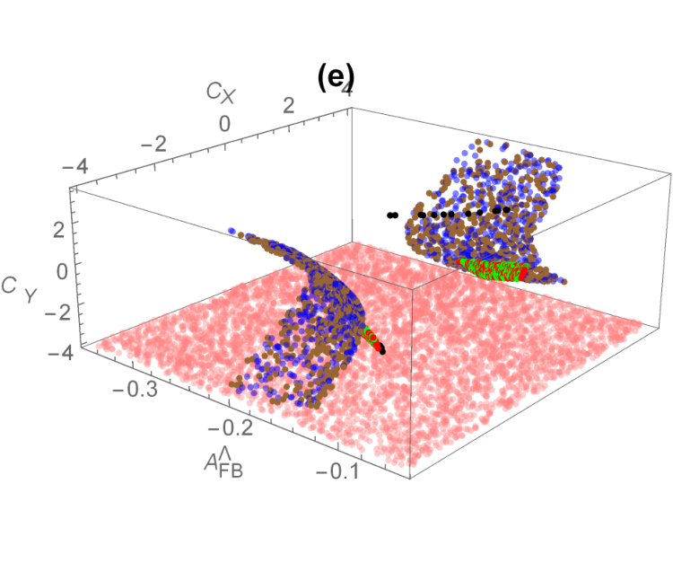
Based on these observations, we can see that taking new couplings separately is not a favorable option in the presence of available data of the different physical observables in Λb→Λ(→pπ−)μ+μ−\Lambda_{b}\to\Lambda(\to p\pi^{-})\mu^{+}\mu^{-} decay. Therefore, it is useful to see if two new couplings are turned on together, does this situation improves or not? In order to do so, the constraints on new WCs corresponding to vector, axial-vector, scalar and pseudo-scalar operators are once again chosen from the one adopted by Das:2018sms and by using the global fit presented in Altmannshofer:2017fio; i.e.,

CV=[−1.61,−1]CS(′)=[−4,4]CP(′)=[−4,4]\displaystyle C_{V}=[-1.61,-1]\hskip 28.45274ptC_{S}^{(\prime)}=[-4,4]\hskip 28.45274ptC_{P}^{(\prime)}=[-4,4] (24)

with |CS,P−CS,P′|≤0.1|C_{S,P}-C_{S,P}^{\prime}|\leq 0.1. We have not included CV′,CA,CA′,CTC_{V}^{\prime},\;C_{A},\;C_{A}^{\prime},\;C_{T} and CT​5C_{T5} in the forthcoming numerical analysis as the severe constraints from B−B-physics on these WCs do not allow us to vary them significantly. Thus, from Eq. (24) the following ten combinations are possible:

(i):(CS,CV),(ii):(CS′,CV),(iii):(CP,CV),(iv):(CP′,CV),(v):(CS,CS′)\displaystyle\text{(i)}:(C_{S},C_{V}),\quad\text{(ii)}:(C_{S}^{\prime},C_{V}),\quad\text{(iii)}:(C_{P},C_{V}),\quad\text{(iv)}:(C_{P}^{\prime},C_{V}),\quad\text{(v)}:(C_{S},C_{S^{\prime}}) (25)
(vi):(CS,CP′),(vii):(CS′,CP),(viii):(CS,CP),(ix):(CS′,CP′),(x):(CP,CP′).\displaystyle\text{(vi)}:(C_{S},C_{P}^{\prime}),\quad\text{(vii)}:(C_{S}^{\prime},C_{P}),\quad\text{(viii)}:(C_{S},C_{P}),\quad\text{(ix)}:(C_{S^{\prime}},C_{P^{\prime}}),\quad\text{(x)}:(C_{P},C_{P}^{\prime}).

Among these combinations, we are interested in looking for the combination(s) which maximally accommodate the current available data of all the four observables mentioned above. With this condition, by exploring the various combinations given in Eq. (25), it is found that there is not a single choice which could explain the full data of all four observables simultaneously. However, we found from Eq. (26) that there are six combinations of new WCs which could accommodate the data of the four observables;, i.e., d​ℬ/d​sd\mathcal{B}/ds, FLF_{L}, AF​BℓA^{\ell}_{FB} and AF​BΛA^{\Lambda}_{FB} simultaneously in the bins s∈[0.1,2]s\in[0.1,2] GeV2 and s∈[15,16]s\in[15,16] GeV2 and three observables (excluding d​ℬ/d​sd\mathcal{B}/ds) in s∈[18,20]s\in[18,20] GeV2 bin. In this case, for the bin s∈[16,18]s\in[16,18] GeV2 only FLF_{L} and AF​BΛA^{\Lambda}_{FB} can be taken care of. On the other hand, if we would like to accommodate the data of d​ℬ/d​sd\mathcal{B}/ds as well, we have to choose one from the other three observables. Therefore, based on these observations the six possible combinations of new couplings which accommodate almost all the data of above mentioned three or four observables simultaneously are

(i):(CS,CV),(ii):(CS′,CV),(iii):(CP′,CV),\displaystyle\text{(i)}:(C_{S},C_{V}),\quad\text{(ii)}:(C_{S}^{\prime},C_{V}),\quad\text{(iii)}:(C_{P}^{\prime},C_{V}),\quad (26)
(iv):(CS,CS′),(v):(CS,CP′),(vi):(CS′,CP)\displaystyle\text{(iv)}:(C_{S},C_{S}^{\prime}),\quad\text{(v)}:(C_{S},C_{P}^{\prime}),\quad\text{(vi)}:(C_{S}^{\prime},C_{P}) .

The impact of these combinations of new couplings on the experimentally measured and other physical observables in low (high-recoil region) and high (low-recoil region) ss bins will be discussed from here onwards. The whole analysis is performed by taking the central values of the FFs and that of the experimental data of d​ℬ/d​sd\mathcal{B}/ds, FLF_{L}, AF​BℓA^{\ell}_{FB} and AF​BΛA^{\Lambda}_{FB}.

4.4.1 High recoil region

In this region, we focus only on the bin s∈[0.1,2]s\in[0.1,2] GeV2 because the LHCb data in this particular region is available for all the four observables mentioned above. First, we have examined all the six combinations given in Eq. (26) by tweaking them in their current allowed ranges (c.f. Eq. (24)), to see if they could simultaneously accommodate the available data of these observables or not. At the next step, we have calculated the values of these observables for these combinations accordingly and their results are presented in Fig. 8. From these plots, we have made the following observations:

Refer to caption    Refer to caption
Refer to caption
Figure 8: (a) The parametric space of (CX,CY)(C_{X},C_{Y}) allowed from B−B-physics constraints on new WCs and that satisfy the data of d​ℬ/d​sd\mathcal{B}/ds, FLF_{L}, AF​BℓA_{FB}^{\ell} and AF​BΛA_{FB}^{\Lambda} simultaneously in the bin s∈[0.1,2]s\in[0.1,2] GeV2. Different colors in the plots represent different combinations of new WCs: Red, blue, green, cyan, brown and black dots represent the (CX,CY)(C_{X},\;C_{Y}) == (CS,CV)(C_{S},\;C_{V}), (CS,CP′)(C_{S},\;C_{P}^{\prime}), (CS′,CV)(C_{S}^{\prime},\;C_{V}), (CP′,CV)(C_{P}^{\prime},\;C_{V}), (CS′,CP)(C_{S}^{\prime},\;C_{P}) and (CS,CS′)(C_{S},\;C_{S}^{\prime}), respectively. The plots (b)-(e) present the predictions of d​ℬ/d​sd\mathcal{B}/ds, FLF_{L}, AF​BℓA_{FB}^{\ell} and AF​BΛA_{FB}^{\Lambda} in the bin s∈[0.1,2]s\in[0.1,2] GeV2 against the WCs collected in (a) where the pink flat curves reflect the measured values of d​ℬ/d​sd\mathcal{B}/ds, FLF_{L}, AF​BΛA_{FB}^{\Lambda} and AF​BℓA_{FB}^{\ell}, along with the uncertainties at the LHCb.
  • •

    Fig. 8(a) reflects the complete range of each combination of new WCs given in Eq. (26) which is allowed by B−B-physics data (c.f. Eq. (24)) with the condition |CS−CS′|≤0.1|C_{S}-C_{S}^{\prime}|\leq 0.1. The range of CXC_{X}, CYC_{Y} and the corresponding color schemes are given in the caption of the figure. We found that the full allowed ranges of WCs from B−B-meson decays simultaneously satisfy the the data of d​ℬ/d​sd\mathcal{B}/ds, FLF_{L}, AF​BℓA_{FB}^{\ell} and AF​BΛA_{FB}^{\Lambda} in s∈[0.1,2]s\in[0.1,2] GeV2 bin.

  • •

    By using these allowed values for each combination of new WCs, we predict the values of d​ℬ/d​sd\mathcal{B}/ds, FLF_{L}, AF​BℓA_{FB}^{\ell} and AF​BΛA_{FB}^{\Lambda} by plotting them against the CXC_{X} and CYC_{Y} in Fig. 8(b)-(e). The pink plane in each plot corresponds to the measured experimental range of the observable. The central SM values of d​ℬ/d​sd\mathcal{B}/ds, FLF_{L}, AF​BℓA_{FB}^{\ell} and AF​BΛA_{FB}^{\Lambda} are 0.24×10−70.24\times 10^{-7}, 0.540.54, 0.100.10 and −0.31-0.31, respectively, in s∈[0.1,2]s\in[0.1,2] GeV2 as shown in Table 1.

  • •

    Fig. 8(b) shows that the value of d​ℬ/d​sd\mathcal{B}/ds varies from 0.27×10−70.27\times 10^{-7} to 0.50×10−70.50\times 10^{-7} inside the experimentally allowed region when CXC_{X} and CYC_{Y} are varied in their range constrained by the analysis of different B−B- meson decays. Hence it can be inferred that the experimentally allowed region 0.22×10⁻⁷<d​ℬ/d​s<0.27×10−70.22\times 10^{-7}<d\mathcal{B}/ds<0.27\times 10^{-7} is excluded by the present analysis.

  • •

    Fig. 8(c) represents the variation in the values of FLF_{L} against each combination of CXC_{X} and CYC_{Y}. It can be noticed that the value of FLF_{L} approximately varies from 0.39−0.770.39-0.77 when we vary the values of CXC_{X} and CYC_{Y} in their allowed ranges. It means current constraints on the new WCs suggest that the value of FLF_{L} is 0.39<FL<0.770.39<F_{L}<0.77 therefore, it excludes the experimental measured ranges that are above and below this range of FLF_{L}.

  • •

    Fig. 8(d) depicts that the value of AF​BℓA^{\ell}_{FB} is not very sensitive to the combinations of NP couplings and its value remains close to its SM prediction which is 0.0970.097 (central value). Therefore, the larger experimental values of this observable can not be accommodated in light of the current constraints on new WCs.

  • •

    In case of AF​BΛA^{\Lambda}_{FB}, the combinations (CP′,CV)(C_{P}^{\prime},\;C_{V}) and (CS,CS′)(C_{S},\;C_{S}^{\prime}) (cyan and black dots) change the value of this observable from its SM predictions to some extent while for other combinations of new WCs this value remains close to the SM predictions and it can be seen in Fig. 8(e). In this high-recoil bin, the maximum and the minimum values of AF​BΛA^{\Lambda}_{FB} are found to be −0.25-0.25 and −0.4-0.4, respectively. Therefore, the positive value of this observable and the value greater than −0.25-0.25 seems to be excluded by the current constraints on these new WCs.

In short, the observables d​ℬ/d​sd\mathcal{B}/ds, FLF_{L}, AF​BℓA_{FB}^{\ell} and AF​BΛA_{FB}^{\Lambda} in high recoil region are very interesting to tell us more about the possible values of the new V​AVA and S​PSP couplings. Particularly, in this bin the study of the observables of Λb\Lambda_{b} decay do not put additional constraints on the range of WCs obtained from the analysis of B−B-meson decays.

4.4.2 Low recoil region

We have already mentioned in Sect. 1 that the QCD uncertainties arising from the non-factorizable part of the amplitude has been neglected in our analysis. In case of the very well studied B→K∗​ℓ+​ℓ−B\to K^{\ast}\ell^{+}\ell^{-} decay, these effects are quite challenging theoretically and it is difficult to control them Bobeth:2017vxj and this is even more daunting task for the Λb→Λ(→pπ)ℓ+ℓ−\Lambda_{b}\to\Lambda(\to p\pi)\ell^{+}\ell^{-} decay. Eventually, these effects may question the NP analysis in q2<mJ/ψ2q^{2}<m^{2}_{J/\psi} region. This is the reason why the most recent phenomenological study carried out on Λb→Λ​ℓ+​ℓ−\Lambda_{b}\to\Lambda\ell^{+}\ell^{-} in connection to B−B-physics anomalies restricts any consideration to the low-recoil region only Blake:2019guk. Due to this reason, we have also attempted to see if we can accommodate the data of d​ℬ/d​sd\mathcal{B}/ds, FLF_{L}, AF​BℓA_{FB}^{\ell} and AF​BΛA_{FB}^{\Lambda} by using the above mentioned constraints on the new WCs.

For the low-recoil bin s∈[15,16]s\in[15,16] GeV2, one can make the following observations from Fig. 9

Refer to caption    Refer to caption
Refer to caption
Figure 9: Plot (a) shows the parametric space of (CX,CY)(C_{X},C_{Y}) allowed from B−B-physics constraints on new WCs and which also satisfy the data of d​ℬ/d​sd\mathcal{B}/ds, FLF_{L}, AF​BℓA_{FB}^{\ell} and AF​BΛA_{FB}^{\Lambda}, simultaneously, in the bin s∈[15,16]s\in[15,16] GeV2. (b)-(e) are the predictions of d​ℬ/d​sd\mathcal{B}/ds, FLF_{L}, AF​BℓA_{FB}^{\ell} and AF​BΛA_{FB}^{\Lambda} in the bin s∈[15,16]s\in[15,16] GeV2 against the WCs collected in (a). The legends are same as Fig. 8.
  • •

    In this bin, the available data of all four observables could be accommodated by the combinations of V​AVA and S​PSP couplings given in Eq. (26) with the exception of (CP′,CV)(C_{P}^{\prime},C_{V}). However, when we try to accommodate the available data of the observables by these combinations the range of new WCs allowed by B−B-physics is further reduced and it can be seen from Fig. 9(a).

  • •

    It can be noticed from the blue and brown dots in Fig. 9(a) that for the combinations (CS,CP′)(C_{S},C_{P}^{\prime}) and (CS′,CP)(C_{S}^{\prime},C_{P}), the parametric space of CSC_{S} is reduced to [±4,±2.6][\pm 4,\pm 2.6] and when CSC_{S} is close to its maximum value, i.e., ±4\pm 4, then full range of CP′∈[+4,−4]C_{P}^{\prime}\in[+4,-4] is allowed. On the other hand when CS′C_{S}^{\prime} is close to ±4\pm 4, the CP′C_{P}^{\prime} is allowed to be varied between [±3,±4][\pm 3,\pm 4] (see brown dots). It can be further seen that if CS(′)C_{S}^{(\prime)} reaches to ±2.6\pm 2.6 then CP′C_{P}^{\prime} goes to zero.

  • •

    In the combinations of (CS(′),CV)(C_{S}^{(\prime)},C_{V}), the parametric space of CVC_{V} is unchanged which can be seen from the red and green dots in Fig. 9(a) while the parametric ranges of CSC_{S}, CS′C_{S}^{\prime} are reduced to ±4<CS<±0.5\pm 4<C_{S}<\pm 0.5 and ±2<CS′<±0.5\pm 2<C_{S}^{\prime}<\pm 0.5 which can be observed from the red and green dots, respectively.

  • •

    The constraint on the combination (CS,CS′)(C_{S},C_{S}^{\prime}) is already severe due to the condition |CS−CS′|≤0.1|C_{S}-C_{S}^{\prime}|\leq 0.1 and it further narrow down when we try to explore the data of above mentioned observables. The new allowed range of this combination is between ±2\pm 2 to ±1\pm 1 with |CS−CS′|≤0.1|C_{S}-C_{S}^{\prime}|\leq 0.1 condition. This can be seen from the black dots in Fig. 9(a).

  • •

    By using these new allowed ranges of model independent WCs, we have predicted the values of all four observables in the bin s∈[15,16]s\in[15,16] GeV2 and plotted them in Fig. 9(b-e). In this bin the SM value of d​ℬ/d​sd\mathcal{B}/ds is 0.80×10−70.80\times 10^{-7} and from Fig. 9(b) we can see that this value varies between (0.82−1.42)×10−7(0.82-1.42)\times 10^{-7} by varying the values of the combinations (CS,CP′)(C_{S},C_{P}^{\prime}), (CS′,CP)(C_{S}^{\prime},C_{P}) and (CS,CS′)(C_{S},C_{S}^{\prime}) in their allowed parametric space shown in Fig. 9(a). It can also be noticed that the combinations (CS,CP′)(C_{S},C_{P}^{\prime}), (CS′,CP)(C_{S}^{\prime},C_{P}) and (CS,CS′)(C_{S},C_{S}^{\prime}) allow full experimental range of d​ℬ/d​sd\mathcal{B}/ds which can be seen by blue, brown and black dots. In contrast to this, the combinations (CS(′),CV)(C_{S}^{(\prime)},C_{V}) allow the region (0.82−1.15)×10−7(0.82-1.15)\times 10^{-7} of experimental measurements that is displayed by red and green dots in the same plot.

  • •

    Just like d​ℬ/d​sd\mathcal{B}/ds, the values of FLF_{L} are also predicted in s∈[15,16]s\in[15,16] GeV2 bin and plotted in Fig. 9(c). The SM value of FLF_{L} is 0.450.45 and it varies in the range 0.19−0.320.19-0.32 for the combinations (CS,CP′)(C_{S},C_{P}^{\prime}), (CS′,CP)(C_{S}^{\prime},C_{P}) and (CS,CS′)(C_{S},C_{S}^{\prime}) (see blue, brown and black dots). On the other hand choosing the combinations (CS(′),CV)(C_{S}^{(\prime)},C_{V}) the value of FLF_{L} does not vary too much and predicted to be about 0.19−0.240.19-0.24. This is displayed by the red and green color dots in the plot.

  • •

    Similarly, the values of AF​BℓA^{\ell}_{FB} are predicted and plotted in Fig. 9(d). The SM value of this observable in this bin is −0.38-0.38 and by using the values of combinations (CS,CP′)(C_{S},C_{P}^{\prime}) and (CS′,CP)(C_{S}^{\prime},C_{P}) it varies between −0.15-0.15 to −0.26-0.26 which is shown by blue and brown dots. For the combinations (CS(′),CV)(C_{S}^{(\prime)},C_{V}), the predicted range of the value of AF​BℓA^{\ell}_{FB} is −0.19-0.19 to −0.12-0.12 (red and green dots).

  • •

    Fig. 9(e) represents the predicted values of AF​BΛA^{\Lambda}_{FB} by using the combinations of new WCs. The SM value of this observable in this bin is −0.31-0.31 and by using the allowed values of (CS,CP′)(C_{S},C_{P}^{\prime}) and (CS′,CP)(C_{S}^{\prime},C_{P}) combinations, it changes from −0.22-0.22 to −0.13-0.13 (blue and brown dots) and by (CS(′),CV)(C_{S}^{(\prime)},C_{V}) combinations the range of the value of AF​BΛA^{\Lambda}_{FB} is found to be −0.17-0.17 to −0.12-0.12 (red and green dots).

It is important to mention here that the values of the observables do not depend on the signs of the new WCs and it can be observed from Fig. 9(b - e). However, when more precise data will be available from the Run 3 of the LHC, we expect that the values of the observables in this bin can be used to further constraining the new WCs particularly, the scalar type couplings.

In s∈[16,18]s\in[16,18] GeV2 bin:

  • •

    The SM values of the d​ℬ/d​sd\mathcal{B}/ds, FLF_{L}, AF​BℓA_{FB}^{\ell} and AF​BΛA_{FB}^{\Lambda} in this bin are 0.82×10−70.82\times 10^{-7}, 0.420.42, −0.38-0.38 and −0.29-0.29, respectively. As we have mentioned earlier that we are interested only in those bins where all four and if not at least three observables could be accommodated simultaneously by using the parametric space of new WCs which is allowed by the B−B-physics data. In this particular bin we have found that only the data of two observables, FLF_{L} and AF​BℓA^{\ell}_{FB} favor our choice. Therefore, based on this fact we can say that this region is not good to predict the values of different angular observables. However, in future when more accurate data will be available in this range of ss it will be look for the possible NP effects due to these new WCs in the decay under consideration.

   Refer to caption
Refer to caption    Refer to caption
Figure 10: Plot (a) shows the parametric space of (CX,CY)(C_{X},C_{Y}) allowed from BB-physics constraints on the new WCs which also satisfy the data of FLF_{L}, AF​BℓA_{FB}^{\ell} and AF​BΛA_{FB}^{\Lambda} simultaneously in the bin s∈[18−20]s\in[18-20] GeV2. (b)-(d) are the predictions of FLF_{L}, AF​BℓA_{FB}^{\ell} and AF​BΛA_{FB}^{\Lambda} in the bin s∈[18−20]s\in[18-20] GeV2 against the WCs collected in (a). The legends are same as Fig. 8.

In s∈[18−20]s\in[18-20] GeV2 bin:

In this bin, by excluding the data of FLF_{L} the available data of remaining three observables; i.e., d​ℬ/d​sd\mathcal{B}/ds, AF​BℓA_{FB}^{\ell} and AF​BΛA_{FB}^{\Lambda} could be accommodated simultaneously for the combinations of new WCs given in Eq. (26). However, except (CS,CP′)(C_{S},C_{P}^{\prime}) and (CP′,CV)(C_{P}^{\prime},C_{V}) the other four combinations of new WCs can take care of LHCb data of these observables. We have also explored the case by including the data of FLF_{L} but in this situation it is found that only one more observable can be accommodated at a time with it. Furthermore, as a result of satisfying the data, this bin provide more severe constraints on the new WCs that are still allowed by B−B-physics and it can be seen from Fig. 10(a). The important observations in this case are the following:

  • •

    It can be noticed from the brown dots in Fig. 10(a) that for the combination (CS′,CP)(C_{S}^{\prime},C_{P}) the parametric space of CS′C_{S}^{\prime} is reduced to [±4,±2.4][\pm 4,\pm 2.4] and that of CPC_{P} is [+3,−3][+3,-3] with the severe parabolic condition 5.057​(CS′−2.384)≃CP25.057(C_{S}^{\prime}-2.384)\simeq C_{P}^{2}. On the other hand, for the other combinations the allowed region of CS(′)C_{S}^{(\prime)} is further narrow down (black and brown dots) while the region of CVC_{V} still remains the same as restricted by B−B-physics data (red and green dots). Therefore, similar to the s∈[15,16]s\in[15,16] GeV2 bin, the s∈[18−20]s\in[18-20] GeV2 is also important for the scalar type new WCs.

  • •

    By using the allowed ranges of new WCs shown in Fig. 10(a) and discussed above, the predictions of the observables d​ℬ/d​sd\mathcal{B}/ds, AF​BℓA_{FB}^{\ell} and AF​BΛA_{FB}^{\Lambda} are plotted in Fig. 10(b-d) in s∈[18−20]s\in[18-20] GeV2 bin. In this bin the SM value of d​ℬ/d​sd\mathcal{B}/ds is 0.66×10−70.66\times 10^{-7} and it can be observed from Fig. 10(b) that by using the allowed values of (CS′,CP)(C_{S}^{\prime}\;,C_{P}) and (CS,CS′)(C_{S},\;C_{S}^{\prime}) combinations, the value of d​ℬ/d​sd\mathcal{B}/ds varies in a very small region of experimental range, i.e., roughly (1.47−1.54)×10−7(1.47-1.54)\times 10^{-7} (brown and black dots, respectively). In contrast, the combinations (CS(′),CV)(C_{S}^{(\prime)},\;C_{V}) allow the full region of experimental values and in this case the range of the value is found to be (0.94−1.54)×10−7(0.94-1.54)\times 10^{-7} that is displayed by the red and green dots in Fig. 10(b).

  • •

    Similarly, the values of AF​BℓA^{\ell}_{FB} are predicted and plotted in Fig. 10(c). The SM value of AF​BℓA^{\ell}_{FB} in this bin is −0.32-0.32 and by using the allowed values of the combinations (CS′,CP)(C_{S}^{\prime},C_{P}) and (CS,CS′)(C_{S},C_{S}^{\prime}) the value is found to be ≃−0.13\simeq-0.13 which is shown by brown and black dots. For the combinations (CS(′),CV)(C_{S}^{(\prime)},C_{V}) the predicted range of AF​BℓA^{\ell}_{FB} is −0.07-0.07 to −0.14-0.14 which is plotted by red and green dots. One can further notice that the allowed range of combinations predict only the negative value of AF​BℓA^{\ell}_{FB} which satisfies a very small experimental region of this observable, particularly, the positive experimental value of this observable is not possible to accommodate if we use the above six combinations.

  • •

    Fig. 10(d) represents the predicted values of AF​BΛA^{\Lambda}_{FB} by using the combinations of new WCs. The SM value of AF​BΛA^{\Lambda}_{FB} in this particular bin is −0.23-0.23 and by using the allowed values of (CS′,CP)(C_{S}^{\prime},C_{P}) and (CS,CS′)(C_{S},C_{S}^{\prime}) combinations, this value is roughly to be −0.10-0.10 (see the brown and black dots) and by (CS(′),CV)(C_{S}^{(\prime)},C_{V}) combinations its values change from −0.07-0.07 to −0.12-0.12 which can be seen by the red and green dots. The higher experimental values of this observable is also not possible to be reproduced by using the current constraints on any possible combination of new WCs.

To summarize, in this particular bin, the analysis of above mentioned observables helps us to put the additional constraints on the new scalar type couplings. On the other hand, the parametric space of the vector type couplings does not change and remains to be the same as constrained by the B−B-physics data. Moreover, similar to the case of s∈[15,16]s\in[15,16] GeV2 bin, the numerical values of the observables in this case are also independent of the sign of new WCs.

4.5 Lepton mass effects

It has already been mentioned that we have calculated the expressions of different physical observables by taking the mass of final state leptons to be non-zero which is not the case in Das:2018sms and hence our study can be easily extended to the semileptonic Λb→Λ​τ+​τ−\Lambda_{b}\to\Lambda\tau^{+}\tau^{-} case. Based on our analysis of Λb→Λ​μ+​μ−\Lambda_{b}\to\Lambda\mu^{+}\mu^{-} we find that μ−\mu-mass effects in the angular observables of the four body decay Λb→Λ(→pπ−)μ+μ−\Lambda_{b}\to\Lambda(\to p\pi^{-})\mu^{+}\mu^{-} are not prominent consequently in the case of muons, the lepton mass terms can be safely ignored like in Das:2018sms. For the sake of completeness, we have also calculated the values of angular observables in low-recoil region for the case of Λb→Λ(→pπ−)τ+τ−\Lambda_{b}\to\Lambda(\to p\pi^{-})\tau^{+}\tau^{-} decay in SM and also by considering the new WCs corresponding to the model independent approach.

Table 5: Observables with and without lepton mass for the decay Λb→Λ(→pπ)τ+τ−\Lambda_{b}\to\Lambda(\to p\pi)\tau^{+}\tau^{-} in the SM and in different scenarios of NP couplings where the case mℓ≠0m_{\ell}\neq 0 corresponds to mℓ=mτm_{\ell}=m_{\tau} in s∈[15,20]s\in[15,20] GeV2 bin. Scenario V​A−1VA-1 corresponds to CV=−1.61C_{V}=-1.61, CV′=CA=CA′=0C_{V}^{\prime}=C_{A}=C_{A}^{\prime}=0, V​A−2VA-2 is the case when CV=−CA=−1C_{V}=-C_{A}=-1, CV′=CA′=0C_{V}^{\prime}=C_{A}^{\prime}=0 and V​A−3VA-3 represent CV=−1.34C_{V}=-1.34, CV′=CA=0C_{V}^{\prime}=C_{A}=0, CA′=−0.4C_{A}^{\prime}=-0.4. Similarly, in S​P−1SP-1 case we have taken CS=CP=−3C_{S}=C_{P}=-3, CS′=CP′=−3.1C_{S}^{\prime}=C_{P}^{\prime}=-3.1 whereas S​P−2SP-2 contain CS=3C_{S}=3, CS′=2.9C_{S}^{\prime}=2.9 and CP=CP′=0C_{P}=C_{P}^{\prime}=0. Tensor couplings correspond to CT=0.72C_{T}=0.72 and CT​5=0.2C_{T5}=0.2.
d​ℬd​s×10−7\frac{d\mathcal{B}}{ds}\times 10^{-7} FL\ \ \ \ \ \ F_{L}\ \ \ \ AF​Bℓ\ \ \ \ A_{FB}^{\ell} AF​BΛ\ \ \ \ \ A_{FB}^{\Lambda}\ \ AF​Bℓ​Λ\ \ \ A_{FB}^{\ell\Lambda} FT\ \ \ \ \ F_{T}
S​Mmℓ=0SM_{m_{\ell=0}} 0.75\ \ \ \ 0.75 0.41\ \ \ \ 0.41 −0.35\ -0.35 −0.26\ -0.26    0.140.14 0.60\ \ \ 0.60
S​Mmℓ≠0SM_{m_{\ell\neq 0}}    0.530.53    0.350.35 −0.13-0.13 −0.26-0.26    0.060.06    0.650.65
V​A−1mℓ=0VA-1_{m_{\ell=0}}    0.520.52    0.400.40 −0.28-0.28 −0.26-0.26    0.120.12    0.600.60
V​A−1mℓ≠0VA-1_{m_{\ell\neq 0}}    0.370.37    0.350.35 −0.11-0.11 −0.26-0.26    0.040.04 0.65\ \ \ 0.65
V​A−2mℓ=0VA-2_{m_{\ell=0}}    0.420.42    0.410.41 −0.35-0.35 −0.26-0.26    0.140.14    0.590.59
V​A−2mℓ≠0VA-2_{m_{\ell\neq 0}}    0.290.29    0.350.35 −0.13-0.13 −0.26-0.26    0.060.06 0.65\ \ \ 0.65
V​A−3mℓ=0VA-3_{m_{\ell=0}}    0.520.52    0.410.41 −0.33-0.33 −0.28-0.28    0.130.13    0.590.59
V​A−3mℓ≠0VA-3_{m_{\ell\neq 0}}    0.360.36    0.350.35 −0.12-0.12 −0.28-0.28    0.050.05 0.65\ \ \ 0.65
S​P−1mℓ=0SP-1_{m_{\ell=0}}    0.910.91    0.220.22 −0.20-0.20 −0.15-0.15    0.140.14    0.590.59
S​P−1mℓ≠0SP-1_{m_{\ell\neq 0}}    0.680.68    0.150.15 −0.05-0.05 −0.12-0.12    0.030.03 0.85\ \ \ 0.85
S​P−2mℓ=0SP-2_{m_{\ell=0}}    0.870.87    0.160.16 −0.14-0.14 −0.11-0.11    0.060.06    0.840.84
S​P−2mℓ≠0SP-2_{m_{\ell\neq 0}}    0.900.90    0.210.21 −0.08-0.08 −0.16-0.16    0.030.03 0.79\ \ \ 0.79
Tmℓ=0′T^{\prime}_{m_{\ell=0}}    0.790.79    0.390.39 −0.33-0.33 −0.25-0.25
Tmℓ≠0′T^{\prime}_{m_{\ell\neq 0}}    0.540.54    0.340.34 −0.13-0.13 −0.26-0.26
Table 6: Observables by taking the massive and massless τ\tau in Λb→Λ(→pπ)τ+τ−\Lambda_{b}\to\Lambda(\to p\pi)\tau^{+}\tau^{-} decay in the SM and also in different NP scenarios. Description of couplings is similar to Table 5.
Y3​s​c×10−3Y_{3sc}\times 10^{-3} Y4​s​c×10−2Y_{4sc}\times 10^{-2}    Y2Y_{2}    αθΛ\alpha_{\theta_{\Lambda}}    αθℓ\alpha_{\theta_{\ell}}    αθℓ′\alpha_{\theta_{\ell}}^{\prime}
S​Mmℓ=0SM_{m_{\ell=0}}    0.020.02    −0.96-0.96    0.020.02 −0.82-0.82 −0.15-0.15    −0.67-0.67
S​Mmℓ≠0SM_{m_{\ell\neq 0}}    0.000.00    −0.19-0.19    0.000.00 −0.82-0.82 −0.03-0.03 −0.26\ -0.26
V​A−1mℓ=0VA-1_{m_{\ell=0}}    0.020.02    −0.94-0.94    0.020.02 −0.82-0.82 −0.15-0.15 −0.54-0.54
V​A−1mℓ≠0VA-1_{m_{\ell\neq 0}}    0.000.00    −0.18-0.18    0.000.00 −0.82-0.82 −0.03-0.03 −0.21\ -0.21
V​A−2mℓ=0VA-2_{m_{\ell=0}}    0.030.03    −1.00-1.00    0.020.02 −0.82-0.82 −0.16-0.16 −0.67-0.67
V​A−2mℓ≠0VA-2_{m_{\ell\neq 0}}    0.000.00    −0.19-0.19    0.000.00 −0.82-0.82 −0.03-0.03 −0.26\ -0.26
V​A−3mℓ=0VA-3_{m_{\ell=0}}    0.020.02    −1.00-1.00    0.020.02 −0.87-0.87 −0.16-0.16 −0.62-0.62
V​A−3mℓ≠0VA-3_{m_{\ell\neq 0}}    0.000.00    −0.19-0.19    0.000.00 −0.87-0.87 −0.03-0.03 −0.24\ -0.24
S​P−1mℓ=0SP-1_{m_{\ell=0}}    0.010.01    −0.10-0.10    0.010.01 −0.46-0.46 −0.05-0.05 −0.21-0.21
S​P−1mℓ≠0SP-1_{m_{\ell\neq 0}}    0.000.00    −0.07-0.07    0.000.00 −0.32-0.32 −0.01-0.01 −0.05\ -0.05
S​P−2mℓ=0SP-2_{m_{\ell=0}}    0.010.01    −0.50-0.50    0.010.01 −0.34-0.34 −0.03-0.03 −0.13-0.13
S​P−2mℓ≠0SP-2_{m_{\ell\neq 0}}    0.000.00    −0.11-0.11    0.000.00 −0.51-0.51 −0.01-0.01 −0.09-0.09
Table 7: Observables by taking the massive and massless τ\tau in Λb→Λ(→pπ)τ+τ−\Lambda_{b}\to\Lambda(\to p\pi)\tau^{+}\tau^{-} decay in the SM and also in different NP scenarios. Description of couplings is similar to Table 5.
αξ\ \ \ \ \ \alpha_{\xi}\ \ \ \ αξ′×10−3\alpha_{\xi}^{\prime}\times 10^{-3} αU\ \ \ \ \alpha_{U}\ \ \ αL\ \ \ \alpha_{L}\ \ \ \ 𝒫3\ \ \ \ \mathcal{P}_{3}\ \ \ 𝒫8\ \ \ \ \mathcal{P}_{8}\ \ \ \ \ 𝒫9\ \ \ \ \mathcal{P}_{9}\ \ \ \
S​Mmℓ=0SM_{m_{\ell=0}}    −0.32-0.32 −0.20\ \ -0.20 −0.79-0.79 −0.84\ -0.84    0.380.38 −0.94-0.94 −0.60-0.60
S​Mmℓ≠0SM_{m_{\ell\neq 0}}    −0.13-0.13 −0.07-0.07 −0.82-0.82 −0.83-0.83    0.140.14 −0.35-0.35 −0.69-0.69
V​A−1mℓ=0VA-1_{m_{\ell=0}}    −0.26-0.26 −0.29-0.29 −0.79-0.79 −0.84\ -0.84    0.310.31 −0.76-0.76 −0.60-0.60
V​A−1mℓ≠0VA-1_{m_{\ell\neq 0}}    −0.11-0.11 −0.11-0.11 −0.82-0.82 −0.83-0.83    0.120.12 −0.29-0.29 −0.69-0.69
V​A−2mℓ=0VA-2_{m_{\ell=0}}    −0.32-0.32 −0.27-0.27 −0.79-0.79 −0.84\ -0.84    0.370.37 −0.94-0.94 −0.59\ -0.59
V​A−2mℓ≠0VA-2_{m_{\ell\neq 0}}    −0.13-0.13 −0.01-0.01 −0.82-0.82 −0.83-0.83    0.150.15 −0.36-0.36 −0.58-0.58
V​A−3mℓ=0VA-3_{m_{\ell=0}}    −0.25-0.25 −4.69-4.69 −0.85-0.85 −0.89\ -0.89    0.340.34 −0.87-0.87 −0.64-0.64
V​A−3mℓ≠0VA-3_{m_{\ell\neq 0}}    −0.10-0.10 −1.78-1.78 −0.87-0.87 −0.88-0.88    0.130.13 −0.33-0.33 −0.73-0.73
S​P−1mℓ=0SP-1_{m_{\ell=0}}    −0.16-0.16 −0.12-0.12 −0.21-0.21 −0.26\ -0.26    0.200.20 −0.52-0.52 −0.34-0.34
S​P−1mℓ≠0SP-1_{m_{\ell\neq 0}}    −0.05-0.05 −0.03-0.03 −0.14-0.14 −0.14\ -0.14    0.060.06 −0.14-0.14 −0.27\ -0.27
S​P−2mℓ=0SP-2_{m_{\ell=0}}    −0.12-0.12 −0.08-0.08 −0.13-0.13 −0.16\ -0.16    0.150.15 −0.37-0.37 −0.24-0.24
S​P−2mℓ≠0SP-2_{m_{\ell\neq 0}} −0.07\ \ -0.07 −0.05\ -0.05 −0.28\ -0.28 −0.30\ -0.30 0.09\ \ 0.09 −0.21\ -0.21 −0.44\ -0.44

By using the central values of the FFs the calculated values of different physical observables are listed in Tables 5 - 7. From the first row in each of the Tables 5 - 7, one can notice that the magnitude of the SM values of observables AF​BℓA_{FB}^{\ell}, FTF_{T}, Y4​s​cY_{4sc}, αθℓ\alpha_{\theta_{\ell}}, αθℓ′\alpha^{\prime}_{\theta_{\ell}}, αξ\alpha_{\xi}, αξ′\alpha_{\xi}^{\prime} and P8P_{8} are increased due to the non-zero τ\tau’s mass whereas the values of AF​BΛA_{FB}^{\Lambda} and αθΛ\alpha_{\theta_{\Lambda}} do not receive tauon mass effect. Similar effects can also be noticed in these tables when we include the V​AVA (rows 2 - 4) and TT (row 7) couplings along with the SM couplings. It is noticed that in the case of S​P−1SP-1, the values of FL,AF​Bℓ,AF​BΛ,FT,Y4​s​c,αθΛ,αθℓ,αθℓ′,αξ,αξ′,αL,P8F_{L},\;A_{FB}^{\ell},\;A_{FB}^{\Lambda},\;F_{T},\;Y_{4sc},\;\alpha_{\theta_{\Lambda}},\;\alpha_{\theta_{\ell}},\;\alpha_{\theta_{\ell}}^{\prime},\alpha_{\xi},\;\alpha_{\xi}^{\prime},\;\alpha_{L},\;P_{8} and P9P_{9} increase when tau mass effects are included whereas d​ℬ/d​s,AF​Bℓ​Λ,αUd\mathcal{B}/ds,\;A_{FB}^{\ell\Lambda},\;\alpha_{U} and P3P_{3} values decrease.

For the second possibility of scalar couplings (S​P−2)(SP-2), the values of the observables AF​Bℓ,A_{FB}^{\ell},, Y4​s​cY_{4sc}, αθℓ\alpha_{\theta_{\ell}}, αθℓ′\alpha_{\theta_{\ell}}^{\prime}, αξ\alpha_{\xi}, αξ′\alpha^{\prime}_{\xi}, αU\alpha_{U} and P8P_{8} are increased due to the τ\tau mass while the values of the observables d​ℬ/d​sd\mathcal{B}/ds, FLF_{L}, AF​BΛA^{\Lambda}_{FB}, AF​Bℓ​ΛA^{\ell\Lambda}_{FB}, FTF_{T}, αθΛ\alpha_{\theta_{\Lambda}}, αL\alpha_{L}, P3P_{3} and P9P_{9} are decreased. However, there are no effects of non-zero tauon mass observed in the calculated values of Y2Y_{2} and Y3​s​cY_{3sc} in both scenarios of SP couplings (c.f. sixth row of Table 7). In short, we have found that the effects of τ\tau mass are significantly large in the decay Λb→Λ(→pπ)τ+τ−\Lambda_{b}\to\Lambda(\to p\pi)\tau^{+}\tau^{-} therefore, in contrast to the case of muons, to pursue the NP effects in the angular observables of Λb→Λ(→pπ)τ+τ−\Lambda_{b}\to\Lambda(\to p\pi)\tau^{+}\tau^{-} decay it is indispensable to include the lepton mass terms in the expressions of different physical observables. Consequently, it is worthy to derive the expressions by taking the lepton mass to be non zero in the semileptonic decay Λb→Λ(→pπ)ℓ+ℓ−\Lambda_{b}\to\Lambda(\to p\pi)\ell^{+}\ell^{-} where ℓ=e,μ,τ\ell=e,\mu,\tau.

4.6 Most favorable pair of Wilson coefficients

We have extracted the most favorable pair of new WC’s which is (CS′,CP)(C_{S}^{\prime},C_{P}) as shown in Fig. 11. This pair satisfy individual observables d​ℬd​s,FL,AF​Bℓ\frac{d\mathcal{B}}{ds},\;F_{L},\;A_{FB}^{\ell} and AF​BΛA_{FB}^{\Lambda} in large-recoil bin s∈[0.1,2]s\in[0.1,2] GeV2 and low-recoil bins s∈[15,16]s\in[15,16] GeV2, [16,18][16,18] GeV2 and [18,20][18,20] GeV2. It means that it can satisfy all experimental data available for Λb\Lambda_{b} decay observables respecting the B−B-physics constraints. Density of plots in Fig. 11 shows how the respective parametric space of (CS′,CP)(C_{S}^{\prime},C_{P}) is favorable by these decay observables.

Refer to caption
Figure 11: (CS′,CP)(C_{S}^{\prime},C_{P}) is the most favorable pair of Wilson coefficients. Green, Black, red and blue colors denote d​ℬd​s,FL,AF​Bℓ\frac{d\mathcal{B}}{ds},\;F_{L},\;A_{FB}^{\ell} and AF​BΛA_{FB}^{\Lambda} respectively.

5 Summary and Conclusion

Here, our investigation on NP is not restricted to operators that already appear in the SM; i.e., the four-fermion ones built out of V−AV-A b→sb\to s and vector/axial leptonic currents - but actually also considers (pseudo)scalar and tensor operators, and the V+AV+A combination for the b→sb\to s current. In literature it is known as the model independent approach. By taking the most general weak interaction Hamiltonian, we have discussed the impact of new V​AVA, S​PSP and tensor TT couplings on above mentioned physical observables in Λb→Λ(→pπ−)μ+μ−\Lambda_{b}\to\Lambda(\to p\pi^{-})\mu^{+}\mu^{-} decay. Most of them are the ratios of angular coefficients and hence show little dependence on the uncertainties involved in the calculation of hadronic FFs therefore, in future these observables can serve as a tool to look for the imprints of currents which are beyond the SM physics.

First of all we have plotted d​ℬ/d​sd\mathcal{B}/ds, AF​BℓA_{FB}^{\ell}, AF​BΛA_{FB}^{\Lambda}, AF​Bℓ​ΛA_{FB}^{\ell\Lambda}, FL,TF_{L,T}, Y2, 3​s​c, 4​s​cY_{2,\;3sc,\;4sc}, 𝒫3, 8, 9\mathcal{P}_{3,\;8,\;9} and α(′)i\alpha^{(\prime)}_{i} where, i=θℓ,θΛ,ξ,L,Ui=\theta_{\ell},\;\theta_{\Lambda},\;\xi,\;L,\;U by considering the non-zero mass for the final state leptons. We deduce that in case of μ\mu as final state lepton the mass effects are negligible at low-recoil for all the observables - but mildly effected some observables, such as FTF_{T}, αθℓ\alpha_{\theta_{\ell}}, Y2Y_{2}, Y4​s​cY_{4sc} and 𝒫9\mathcal{P}_{9} in high-recoil region. Therefore, based on our analysis it can be inferred that one can safely ignore the muon mass terms in the expressions of the lepton helicity fractions as was done in Das:2018sms. By using the following ranges of new WCs that are allowed by the B−B-physics data with the global fit sign suggestions

CV\displaystyle C_{V} =\displaystyle= [−1.61,−1],CV′=0,CA=1,CA′=−0.4\displaystyle[-1.61,-1],\hskip 28.45274ptC_{V}^{\prime}=0,\hskip 28.45274ptC_{A}=1,\hskip 28.45274ptC_{A}^{\prime}=-0.4
CS(′)\displaystyle C_{S}^{(\prime)} =\displaystyle= CP(′)=[−4,4],CT=0.72,CT​5=0.2,\displaystyle C_{P}^{(\prime)}=[-4,4],\hskip 19.91684ptC_{T}=0.72,\hskip 11.38092ptC_{T5}=0.2, (27)

we have the following findings:

  • •

    There is a mismatch between the SM predictions and the LHCb data of d​ℬ/d​sd\mathcal{B}/ds particularly in high ss region. Only new V​AVA couplings in three low ss bins, [0.1,2][0.1,2] GeV2, [2,4][2,4]GeV2 and [6,8][6,8]GeV2 are able to accommodate this data.

  • •

    The SM values of FLF_{L} and AF​BΛA^{\Lambda}_{FB} fall within the error bars of the LHCb data in all bins except in s∈[16,18]s\in[16,18] GeV2 where V​AVA, S​PSP and TT couplings are also unable to accommodate the data.

  • •

    The data of AF​BℓA^{\ell}_{FB} deviates from the SM values in high ss region and only S​PSP couplings show some promising effect to accommodate it.

It is also observed that the zero-crossing of observables shift towards high ss region when new V​AVA couplings are introduced in addition to the SM WCs which is not the case for the S​PSP couplings. In case of αθℓ,αU\alpha_{\theta_{\ell}},\alpha_{U} and αL\alpha_{L} when we include V​AVA couplings their values are modified slightly for the combination CV=−1.34,CA′=−0.4C_{V}=-1.34,C_{A}^{\prime}=-0.4, CV′=CA=0C_{V}^{\prime}=C_{A}=0. However, the data of AF​BℓA_{FB}^{\ell}, particularly in high ss region favors the new V​AVA couplings in comparison to the SM couplings alone. Now compared to V​AVA and TT couplings, the constraints are less stringent on S​PSP WCs therefore, their influence on above discussed observables is more prominent. Also, the data of d​ℬ/d​sd\mathcal{B}/ds, AF​BℓA_{FB}^{\ell} and AF​BΛA_{FB}^{\Lambda} in some high ss bins favor the S​PSP couplings. In case of the WCs corresponding to the tensor currents the value of AF​BΛA_{FB}^{\Lambda} in high ss region come closer to the experimental value which is neither the case for the SM nor for any other NP couplings. Hence, one can deduce that there is not a single new coupling among V​AVA, S​PSP and TT operators that can simultaneously accommodate the whole available LHCb data of these four observables in all ss bins.

To overcome this difficulty, we have also examined the impact of CVC_{V}, CSC_{S}, CS′C_{S}^{\prime}, CPC_{P} and CP′C_{P}^{\prime} by considering these couplings in pairs (CX,CY)(C_{X},C_{Y}) where X,Y=V,S,S′,P,P′X,Y=V,S,S^{\prime},P,P^{\prime}. The goal was to explore their allowed parametric space to see whether the combinations of these new couplings satisfy the available LHCb data for all the four observables in large-recoil bin s∈[0.1,2]s\in[0.1,2] GeV2 and in low-recoil bins s∈[15,16],[16,18]s\in[15,16],\;[16,18] GeV2 and s∈[18,20]s\in[18,20] GeV2 or not. We observed that at large-recoil s∈[0.1,2]s\in[0.1,2] GeV2 region, the measured values of d​ℬ/d​sd\mathcal{B}/ds, FLF_{L}, AF​BℓA_{FB}^{\ell} and AF​BΛA_{FB}^{\Lambda} could be justified simultaneously by taking the combinations given in Eq. (26) while the ranges of WCs mentioned in Eq. (27) remain unchanged. At low-recoil, for the bin s∈[15,16]s\in[15,16] GeV2, these combinations also accommodate LHCb data for all four observables simultaneously but the ranges of S​PSP WCs mentioned in Eq. (27) are further constrained while the ranges of V​AVA WCs remain the same. It reflects that these two bins can provide a good opportunity to search for the NP when more accurate data will be available from the Run 3 of the LHC. In the s∈[16,18]s\in[16,18] GeV2 bin, the measurements of all observables cannot be accommodated by any of the combinations of NP WCs. In this region, only a few combinations satisfy the measured ranges of FLF_{L} and AF​BΛA_{FB}^{\Lambda} simultaneously but none of them satisfy AF​BℓA_{FB}^{\ell}. In last bin of low-recoil region; i.e., s∈[18,20]s\in[18,20] GeV2 we tried to accommodate the data of AF​BℓA_{FB}^{\ell}, AF​BΛA_{FB}^{\Lambda} and d​ℬ/d​sd\mathcal{B}/ds simultaneously and found that it is still possible for the several combinations of NP WCs. However, doing so for these three observables we got more severe constraints on the the S​PSP WCs as compared to the one in s∈[15,16]s\in[15,16] GeV2 bin while the range of V​AVA WCs remains the same as allowed by the BB-physics data. Finally, by using the allowed parametric space of these WCs constrained by the data of above mentioned observables in Λb\Lambda_{b} decays, we predicted the values of these four observables in their corresponding bins and find that they could be potentially measured in future at the LHCb and other planned experiments.

It has already been discussed that in this study we have calculated the expressions of the lepton helicity fractions in the presence of lepton mass therefore, this analysis can be easily extended to the Λb→Λ​τ+​τ−\Lambda_{b}\to\Lambda\tau^{+}\tau^{-} decays. Doing so, we found that the non-zero mass of tauons significantly modify the values of different physical observables both in the SM as well as in the presence of new WCs. Finally, by considering the uncertainties involved in the FFs and other input parameters, we have calculated the values of all the 19 observables for Λb→Λ(→pπ−)τ+τ−\Lambda_{b}\to\Lambda(\to p\pi^{-})\tau^{+}\tau^{-} decay.

Appendix

Helicity amplitudes for hardronic part

It is well known fact that the helicity formalism provide a convenient way to find the projections of Λb→Λ\Lambda_{b}\to\Lambda matrix elements on the direction of the polarization of virtual gauge boson Gutsche:2013pp; Boer:2014kda; Yan:2019tgn. In case of vector currents, we can write

HVt(sΛb,sΛ)=εtμ∗⟨Λ(PΛ,sΛ)|s¯γμb|Λ(PΛb,sΛb)⟩H_{V}^{t}(s_{\Lambda_{b}},\;s_{\Lambda})=\varepsilon^{\mu*}_{t}\langle\Lambda(P_{\Lambda},s_{\Lambda})|\bar{s}\gamma^{\mu}b|\Lambda(P_{\Lambda_{b}},s_{\Lambda_{b}})\rangle (28)

where ϵμ∗t\epsilon^{\mu*}_{t} denotes the time-like polarization of the virtual gauge boson and sΛbs_{\Lambda_{b}} and sΛs_{\Lambda} are the spin-projections of initial and final state baryons on the z−z-axis in their rest frames, respectively. Using Eq. (5) and the kinematical relations defined in Das:2018sms; Gutsche:2013pp along with εtμ=1s​(q0, 0, 0,−|q→|)\varepsilon^{\mu}_{t}=\frac{1}{\sqrt{s}}\left(q_{0},\;0,\;0,\;-\left|\vec{q}\right|\right), the non-zero helicity components for time-like polarization from Eq. (5) read

HVt(+1/2,+1/2)=HVt(−1/2,−1/2)=fVt(s)mΛb−mΛss+.\displaystyle H^{t}_{V}(+1/2,+1/2)=H^{t}_{V}(-1/2,-1/2)=f_{V}^{t}(s)\frac{m_{\Lambda_{b}}-m_{\Lambda}}{\sqrt{s}}\sqrt{s_{+}}. (29)

In case of longitudinal polarization ε0μ∗=1s(|q→|, 0, 0,−q0)\varepsilon^{\mu*}_{0}=\frac{1}{\sqrt{s}}\left(\left|\vec{q}\right|,\;0,\;0,\;-q_{0}\right), the corresponding helicity amplitude becomes

HV0(sΛb,sΛ)=ε0μ∗⟨Λ(PΛ,sΛ)|s¯γμb|Λ(PΛb,sΛb)⟩H_{V}^{0}(s_{\Lambda_{b}},\;s_{\Lambda})=\varepsilon^{\mu*}_{0}\langle\Lambda(P_{\Lambda},s_{\Lambda})|\bar{s}\gamma^{\mu}b|\Lambda(P_{\Lambda_{b}},s_{\Lambda_{b}})\rangle (30)

and using Eq. (5), the non-zero longitudinal components for vector current will take the form

HV0(+1/2,+1/2)=HV0(−1/2,−1/2)=fV0(s)mΛb+mΛss−.H^{0}_{V}(+1/2,+1/2)=H^{0}_{V}(-1/2,-1/2)=f_{V}^{0}(s)\frac{m_{\Lambda_{b}}+m_{\Lambda}}{\sqrt{s}}\sqrt{s_{-}}. (31)

with s−=(mΛb−mΛ)2−ss_{-}=(m_{\Lambda_{b}}-m_{\Lambda})^{2}-s. Likewise, for the transverse polarization ε±μ∗=12(0,±1,i,−q0)\varepsilon^{\mu*}_{\pm}=\frac{1}{\sqrt{2}}\left(0,\;\pm 1,\;i,\;-q_{0}\right)

HV±(sΛb,sΛ)=ε±μ∗⟨Λ(PΛ,sΛ)|s¯γμb|Λ(PΛb,sΛb)⟩,H_{V}^{\pm}(s_{\Lambda_{b}},\;s_{\Lambda})=\varepsilon^{\mu*}_{\pm}\langle\Lambda(P_{\Lambda},s_{\Lambda})|\bar{s}\gamma^{\mu}b|\Lambda(P_{\Lambda_{b}},s_{\Lambda_{b}})\rangle, (32)

the corresponding non-zero helicity components are

HV+(−1/2,+1/2)=HV−(+1/2,−1/2)=−fV⟂(s)2​s−.H^{+}_{V}({-1/2,+1/2})=H^{-}_{V}(+1/2,-1/2)=-f_{V}^{\perp}(s)\sqrt{2s_{-}}. (33)

In case of axial-vector currents, from Eq. (6) the corresponding non-zero components for time-like, longitudinal and transverse polarizations of virtual boson are

HAt(+1/2,+1/2)\displaystyle H^{t}_{A}(+1/2,+1/2) =\displaystyle= −HAt(−1/2,−1/2)=fAt(s)mΛb+mΛss−,\displaystyle-H^{t}_{A}(-1/2,-1/2)=f_{A}^{t}(s)\frac{m_{\Lambda_{b}}+m_{\Lambda}}{\sqrt{s}}\sqrt{s_{-}}, (34)
HA0(+1/2,+1/2)\displaystyle H^{0}_{A}(+1/2,+1/2) =\displaystyle= −HA0(−1/2,−1/2)=fA0(s)mΛb−mΛss+,\displaystyle-H^{0}_{A}(-1/2,-1/2)=f_{A}^{0}(s)\frac{m_{\Lambda_{b}}-m_{\Lambda}}{\sqrt{s}}\sqrt{s_{+}}, (35)
HA+(−1/2,+1/2)\displaystyle H^{+}_{A}(-1/2,+1/2) =\displaystyle= −HA−(+1/2,−1/2)=−fA⟂(s)2​s+.\displaystyle-H^{-}_{A}(+1/2,-1/2)=-f_{A}^{\perp}(s)\sqrt{2s_{+}}. (36)

For the dipole operators i​s¯​qν​σμ​ν​bi\bar{s}q_{\nu}\sigma^{\mu\nu}b and i​s¯​qν​σμ​ν​γ5​bi\bar{s}q_{\nu}\sigma^{\mu\nu}\gamma_{5}b, the respective transition matrix elements are defined in Eq. (7) and in this particular case the corresponding non-zero helicity components for different polarizations of virtual boson are

HT0(+1/2,+1/2)\displaystyle H^{0}_{T}(+1/2,+1/2) =\displaystyle= HT0(−1/2,−1/2)=−fT0(s)s​s−\displaystyle H^{0}_{T}(-1/2,-1/2)=-f_{T}^{0}(s)\sqrt{ss_{-}} (37)
HT50(+1/2,+1/2)\displaystyle H^{0}_{T_{5}}(+1/2,+1/2) =\displaystyle= HT50(−1/2,−1/2)=fT50(s)s​s+.\displaystyle H^{0}_{T_{5}}({-1/2,-1/2})=f_{T_{5}}^{0}(s)\sqrt{ss_{+}}. (38)

The helicity amplitude corresponding to the tensor current i.e., s¯​σμ​ν​b\bar{s}\sigma^{\mu\nu}b becomes

HT′m,n(sΛb,sΛ)=εmμ∗ϵnμ∗⟨Λ(PΛ,sΛ)|s¯iσμ​νb|Λ(PΛb,sΛb)⟩,\displaystyle H_{T^{\prime}}^{m,n}(s_{\Lambda_{b},}s_{\Lambda})=\varepsilon^{\mu*}_{m}\epsilon^{\mu*}_{n}\langle\Lambda(P_{\Lambda},s_{\Lambda})|\bar{s}i\sigma^{\mu\nu}b|\Lambda(P_{\Lambda_{b}},s_{\Lambda_{b}})\rangle, (39)

where m,n=t,0,±m,n=t,0,\pm. Using the expression of ⟨Λ⁡(PΛ,sΛ)​|s¯​i​σμ​ν​b|​Λb​(PΛb,sΛb)⟩\langle\Lambda\left(P_{\Lambda},\;s_{\Lambda}\right)\left|\bar{s}i\sigma^{\mu\nu}b\right|\Lambda_{b}\left(P_{\Lambda_{b}},\;s_{\Lambda_{b}}\right)\rangle from Das:2018sms (c.f. Eq. (C.7)), the non-zero components for virtual bosons’s time-like, longitudinal, transverse and the possible combination of these polarization becomes

HT′0​t(+1/2,+1/2)\displaystyle H^{0t}_{T^{\prime}}(+1/2,+1/2) =\displaystyle= HT′0​t(−1/2,−1/2)=−fT0(s)s−\displaystyle H^{0t}_{T^{\prime}}(-1/2,-1/2)=-f_{T}^{0}(s)\sqrt{s_{-}} (40)
HT′+t(−1/2,+1/2)\displaystyle H^{+t}_{T^{\prime}}(-1/2,+1/2) =\displaystyle= HT′−t(+1/2,−1/2)=fT5⟂(s)mΛb+mΛs2​s−\displaystyle H^{-t}_{T^{\prime}}(+1/2,-1/2)=f_{T_{5}}^{\perp}(s)\frac{m_{\Lambda_{b}}+m_{\Lambda}}{\sqrt{s}}\sqrt{2s_{-}} (41)
HT′+0(−1/2,+1/2)\displaystyle H^{+0}_{T^{\prime}}(-1/2,+1/2) =\displaystyle= HT′−0(+1/2,−1/2)=fT5⟂(s)mΛb−mΛs2​s+\displaystyle H^{-0}_{T^{\prime}}(+1/2,-1/2)=f_{T_{5}}^{\perp}(s)\frac{m_{\Lambda_{b}}-m_{\Lambda}}{\sqrt{s}}\sqrt{2s_{+}} (42)
HT′+⁣−(+1/2,+1/2)\displaystyle H^{+-}_{T^{\prime}}(+1/2,+1/2) =\displaystyle= −HT′+⁣−(−1/2,−1/2)=−fT50(s)s+\displaystyle-H^{+-}_{T^{\prime}}(-1/2,-1/2)=-f_{T_{5}}^{0}(s)\sqrt{s_{+}} (43)

The remaining components can be obtained by using the relation HT′m,n​(sΛb,sΛ)=−HT′n,m​(sΛb,sΛ)H^{m,n}_{T^{\prime}}(s_{\Lambda_{b}},s_{\Lambda})=-H^{n,m}_{T^{\prime}}(s_{\Lambda_{b}},s_{\Lambda}).

In case of the scalar and pseduo-scalar currents, the corresponding helicity amplitudes along with their non-zero components can be obtained from Eqs. (9) and (10) and these are

HSt(+1/2,+1/2)\displaystyle H^{t}_{S}(+1/2,+1/2) =\displaystyle= HSt(−1/2,−1/2)=fVt(s)mΛb−mΛmbs+,\displaystyle H^{t}_{S}(-1/2,-1/2)=f_{V}^{t}(s)\frac{m_{\Lambda_{b}}-m_{\Lambda}}{m_{b}}\sqrt{s_{+}}, (44)
HPt(+1/2,+1/2)\displaystyle H^{t}_{P}(+1/2,+1/2) =\displaystyle= −HPt(−1/2,−1/2)=−fAt(s)mΛb−mΛmbs−.\displaystyle-H^{t}_{P}(-1/2,-1/2)=-f_{A}^{t}(s)\frac{m_{\Lambda_{b}}-m_{\Lambda}}{m_{b}}\sqrt{s_{-}}. (45)

.1 Helicity amplitudes for lepton-part

Just like the hadronic part, the leptonic helicity amplitudes the scalar (S)(S), pseudo-scalar (P)(P), vector (V)(V) and axial-vector (A)(A) currents having non-zero contribution are Yan:2019tgn

LS(+1/2,+1/2)\displaystyle L_{S}(+1/2,+1/2) =\displaystyle= −LS(−1/2,−1/2)=sβℓ,LP(+1/2,+1/2)=LP(−1/2,−1/2)=−s,\displaystyle-L_{S}(-1/2,-1/2)=s\beta_{\ell},\quad\quad\quad\quad\quad\quad\quad L_{P}(+1/2,+1/2)=L_{P}(-1/2,-1/2)=-s,
LV±(+1/2,+1/2)\displaystyle L_{V}^{\pm}(+1/2,+1/2) =\displaystyle= LV∓(−1/2,−1/2)=∓2mℓsinθℓ,LV0(+1/2,+1/2)=−LV0(−1/2,−1/2)=−2mℓcosθℓ,\displaystyle L_{V}^{\mp}(-1/2,-1/2)=\mp\sqrt{2}m_{\ell}\sin{\theta_{\ell}},\quad\quad\quad\;L_{V}^{0}(+1/2,+1/2)=-L_{V}^{0}(-1/2,-1/2)=-2m_{\ell}\cos\theta_{\ell},
LV0(+1/2,−1/2)\displaystyle L_{V}^{0}(+1/2,-1/2) =\displaystyle= LV0(−1/2,+1/2)=ssinθℓ,LV+(+1/2,−1/2)=−LV−(−1/2,+1/2)=s2(1−cosθℓ),\displaystyle L_{V}^{0}(-1/2,+1/2)=s\sin\theta_{\ell},\quad\quad\quad\quad\quad\quad\;L_{V}^{+}(+1/2,-1/2)=-L_{V}^{-}(-1/2,+1/2)=\frac{s}{\sqrt{2}}(1-\cos\theta_{\ell}),
LV−(+1/2,−1/2)\displaystyle L_{V}^{-}(+1/2,-1/2) =\displaystyle= −LV+(−1/2,+1/2)=s2(1+cosθℓ),LAt(+1/2,+1/2)=LAt(−1/2,−1/2)=−2mℓ,\displaystyle-L_{V}^{+}(-1/2,+1/2)=\frac{s}{\sqrt{2}}(1+\cos\theta_{\ell}),\quad\quad L_{A}^{t}(+1/2,+1/2)=L_{A}^{t}(-1/2,-1/2)=-2m_{\ell},
LA+(+1/2,−1/2)\displaystyle L_{A}^{+}(+1/2,-1/2) =\displaystyle= LA−(−1/2,+1/2)=s​v2(1−cosθℓ),LA−(+1/2,−1/2)=LA+(−1/2,+1/2)=s​v2(1+cosθℓ),\displaystyle L_{A}^{-}(-1/2,+1/2)=\frac{sv}{\sqrt{2}}(1-\cos\theta_{\ell}),\quad\quad\quad L_{A}^{-}(+1/2,-1/2)=L_{A}^{+}(-1/2,+1/2)=\frac{sv}{\sqrt{2}}(1+\cos\theta_{\ell}),
LA0(+1/2,−1/2)\displaystyle L_{A}^{0}(+1/2,-1/2) =\displaystyle= −LA0(−1/2,+1/2)=svsinθℓ.\displaystyle-L_{A}^{0}(-1/2,+1/2)=sv\sin\theta_{\ell}. (46)

Similarly, from the tensor current σμ​ν​(1∓γ5)\sigma_{\mu\nu}(1\mp\gamma_{5}) the non-zero leptonic helicity amplitudes are

LT′t,±(+1/2,+1/2)\displaystyle L_{T^{\prime}}^{t,\pm}(+1/2,+1/2) =\displaystyle= −LT′t,±(−1/2,−1/2)=∓s2sinθℓ,LT′t,+(−1/2,+1/2)=−LT′t,−(+1/2,−1/2)=2(1−cosθℓ)mℓ\displaystyle-L_{T^{\prime}}^{t,\pm}(-1/2,-1/2)=\mp\frac{s}{\sqrt{2}}\sin\theta_{\ell},\;L_{T^{\prime}}^{t,+}(-1/2,+1/2)=-L_{T^{\prime}}^{t,-}(+1/2,-1/2)=\sqrt{2}(1-\cos\theta_{\ell})m_{\ell}
LT′t,−(−1/2,+1/2)\displaystyle L_{T^{\prime}}^{t,-}(-1/2,+1/2) =\displaystyle= −LT′t,+(+1/2,−1/2)=2mℓ(1+cosθℓ),LT′t,0(+1/2,+1/2)=−LT′t,0(−1/2,−1/2)=−scosθℓ\displaystyle-L_{T^{\prime}}^{t,+}(+1/2,-1/2)=\sqrt{2}m_{\ell}(1+\cos\theta_{\ell}),\;L_{T^{\prime}}^{t,0}(+1/2,+1/2)=-L_{T^{\prime}}^{t,0}(-1/2,-1/2)=-s\cos\theta_{\ell}
LT′+,−(+1/2,+1/2)\displaystyle L_{T^{\prime}}^{+,-}(+1/2,+1/2) =\displaystyle= LT′+,−(−1/2,−1/2)=−scosθℓβℓ,LT′±,0(+1/2,+1/2)=LT′±,0(−1/2,−1/2)=−s2sinθℓβℓ,\displaystyle L_{T^{\prime}}^{+,-}(-1/2,-1/2)=-s\cos\theta_{\ell}\beta_{\ell},\;L_{T^{\prime}}^{\pm,0}(+1/2,+1/2)=L_{T^{\prime}}^{\pm,0}(-1/2,-1/2)=-\frac{s}{\sqrt{2}}\sin\theta_{\ell}\beta_{\ell}, (47)
LT′t,0(−1/2,+1/2)\displaystyle L_{T^{\prime}}^{t,0}(-1/2,+1/2) =\displaystyle= LT′t,0(+1/2,−1/2)=2mℓsinθℓ,LT​5′t,±(+1/2,+1/2)=−LT​5′t,±(−1/2,−1/2)=±s2sinθℓβℓ\displaystyle L_{T^{\prime}}^{t,0}(+1/2,-1/2)=2m_{\ell}\sin\theta_{\ell},\;L_{T5^{\prime}}^{t,\pm}(+1/2,+1/2)=-L_{T5^{\prime}}^{t,\pm}(-1/2,-1/2)=\pm\frac{s}{\sqrt{2}}\sin\theta_{\ell}\beta_{\ell}
LT​5′t,0(+1/2,+1/2)\displaystyle L_{T5^{\prime}}^{t,0}(+1/2,+1/2) =\displaystyle= LT​5′t,0(−1/2,−1/2)=scosθℓβℓ,LT​5′+,−(+1/2,+1/2)=−LT​5′+,−(−1/2,−1/2)=scosθℓ,\displaystyle L_{T5^{\prime}}^{t,0}(-1/2,-1/2)=s\cos\theta_{\ell}\beta_{\ell},\;L_{T5^{\prime}}^{+,-}(+1/2,+1/2)=-L_{T5^{\prime}}^{+,-}(-1/2,-1/2)=s\cos\theta_{\ell},
LT​5′−,+(+1/2,−1/2)\displaystyle L_{T5^{\prime}}^{-,+}(+1/2,-1/2) =\displaystyle= LT​5′−,+(−1/2,+1/2)=2mℓsinθℓ,LT​5′+,0(+1/2,−1/2)=−LT​5′−,0(−1/2,+1/2)=2(1+cosθℓ)mℓ,\displaystyle L_{T5^{\prime}}^{-,+}(-1/2,+1/2)=2m_{\ell}\sin\theta_{\ell},\;L_{T5^{\prime}}^{+,0}(+1/2,-1/2)=-L_{T5^{\prime}}^{-,0}(-1/2,+1/2)={\sqrt{2}}(1+\cos\theta_{\ell})m_{\ell},
LT​5′±,0(+1/2,+1/2)\displaystyle L_{T5^{\prime}}^{\pm,0}(+1/2,+1/2) =\displaystyle= −LT​5′±,0(−1/2,−1/2)=s2sinθℓ,LT​5′−,0(+1/2,−1/2)=LT​5′+,0(−1/2,+1/2)=−2(1−cosθℓ)mℓ.\displaystyle-L_{T5^{\prime}}^{\pm,0}(-1/2,-1/2)=\frac{s}{\sqrt{2}}\sin\theta_{\ell},\;L_{T5^{\prime}}^{-,0}(+1/2,-1/2)=L_{T5^{\prime}}^{+,0}(-1/2,+1/2)=-{\sqrt{2}}(1-\cos\theta_{\ell})m_{\ell}.

It can be seen that by setting the lepton mass mℓm_{\ell} to be zero, we can obtain the relations given in Das:2018sms .

In terms of the hadronic and leptonic currents, the square of amplitudes corresponding to different currents can be assembled as

|MV​A|2\displaystyle|M_{VA}|^{2} =\displaystyle= 14∑sΛb,sΛ∑sΛ′∑sℓ1,sℓ2∑m,n∑m′,n′Hm(sΛb,sΛ)Hn∗(sΛb,sΛ′)gm,m′gn,n′Lm′(sℓ1,sℓ2)Ln′∗(sℓ1,sℓ2)Γ′(sΛ,sΛ′),\displaystyle\frac{1}{4}\sum_{s_{\Lambda_{b}},s_{\Lambda}}\sum_{s_{\Lambda}^{\prime}}\sum_{s_{\ell_{1}},s_{\ell_{2}}}\sum_{m,n}\sum_{m^{\prime},n^{\prime}}H^{m}(s_{\Lambda_{b}},s_{\Lambda})H^{n*}(s_{\Lambda_{b}},s_{\Lambda^{\prime}})g_{m,m^{\prime}}g_{n,n^{\prime}}L^{m^{\prime}}(s_{\ell_{1}},s_{\ell_{2}})L^{n^{\prime^{*}}}(s_{\ell_{1}},s_{\ell_{2}})\Gamma^{\prime}(s_{\Lambda},s_{\Lambda}^{\prime}),

where λ=(mΛb2−mΛ2−s)2+4​s​mΛ2\lambda=(m_{\Lambda_{b}}^{2}-m_{\Lambda}^{2}-s)^{2}+4sm_{\Lambda}^{2} and Lm′,n′L^{m^{\prime},\;n^{\prime}} are the helicity amplitudes for the leptonic part given in Eq. (47). Likewise

|MS​P|2\displaystyle|M_{SP}|^{2} =\displaystyle= 14​∑sΛb,sΛ∑sΛ′∑sℓ1,sℓ2H⁡(sΛb,sΛ)​H∗​(sΛb,sΛ′)​L​(sℓ1,sℓ2)​L∗​(sℓ1,sℓ2)​Γ′​(sΛ,sΛ′)\displaystyle\frac{1}{4}\sum_{s_{\Lambda_{b}},s_{\Lambda}}\sum_{s_{\Lambda}^{\prime}}\sum_{s_{\ell_{1}},s_{\ell_{2}}}H(s_{\Lambda_{b}},s_{\Lambda})H^{*}(s_{\Lambda_{b}},s_{\Lambda^{\prime}})L(s_{\ell_{1}},s_{\ell_{2}})L^{*}(s_{\ell_{1}},s_{\ell_{2}})\Gamma^{\prime}(s_{\Lambda},s_{\Lambda}^{\prime})
|MT′|2\displaystyle|M_{T^{\prime}}|^{2} =\displaystyle= ∑sΛb,sΛ∑sΛ′∑sℓ1,sℓ2Hm​n(sΛb,sΛ)Hrs∗(sΛb,sΛ′)gm​m′gn​n′gr​r′gs​s′Lm′​n′(sℓ1,sℓ2)Lr′s′∗(sℓ1,sℓ2)Γ′(sΛ,sΛ′)\displaystyle\sum_{s_{\Lambda_{b}},s_{\Lambda}}\sum_{s_{\Lambda}^{\prime}}\sum_{s_{\ell_{1}},s_{\ell_{2}}}H^{mn}(s_{\Lambda_{b}},s_{\Lambda})H^{rs*}(s_{\Lambda_{b}},s_{\Lambda^{\prime}})g_{mm^{\prime}}g_{nn^{\prime}}g_{rr^{\prime}}g_{ss^{\prime}}L^{m^{\prime}n^{\prime}}(s_{\ell_{1}},s_{\ell_{2}})L^{r^{\prime}s^{\prime}*}(s_{\ell_{1}},s_{\ell_{2}})\Gamma^{\prime}(s_{\Lambda},s_{\Lambda}^{\prime})
MV​A​MS​P∗+h.c.\displaystyle M_{VA}M^{*}_{SP}+h.c. =\displaystyle= 14∑sΛb,sΛ∑sΛ′∑sℓ1,sℓ2[Hm(sΛb,sΛ)H∗(sΛb,sΛ′)Lm′(sℓ1,sℓ2)L∗(sℓ1,sℓ2)+h.c.]Γ′(sΛ,sΛ′)\displaystyle\frac{1}{4}\sum_{s_{\Lambda_{b}},s_{\Lambda}}\sum_{s_{\Lambda}^{\prime}}\sum_{s_{\ell_{1}},s_{\ell_{2}}}\left[H^{m}(s_{\Lambda_{b}},s_{\Lambda})H^{*}(s_{\Lambda_{b}},s_{\Lambda^{\prime}})L^{m^{\prime}}(s_{\ell_{1}},s_{\ell_{2}})L^{*}(s_{\ell_{1}},s_{\ell_{2}})+h.c.\right]\Gamma^{\prime}(s_{\Lambda},s_{\Lambda}^{\prime})
MV​A​MT′∗+h.c.\displaystyle M_{VA}M^{*}_{T^{\prime}}+h.c. =\displaystyle= 12∑sΛb,sΛ∑sΛ′∑sℓ1,sℓ2[Hm(sΛb,sΛ)H∗r​s(sΛb,sΛ′)Lm′(sℓ1,sℓ2)Lr′s′∗(sℓ1,sℓ2)+h.c.]Γ′(sΛ,sΛ′)\displaystyle\frac{1}{2}\sum_{s_{\Lambda_{b}},s_{\Lambda}}\sum_{s_{\Lambda}^{\prime}}\sum_{s_{\ell_{1}},s_{\ell_{2}}}\left[H^{m}(s_{\Lambda_{b}},s_{\Lambda})H^{*rs}(s_{\Lambda_{b}},s_{\Lambda^{\prime}})L^{m^{\prime}}(s_{\ell_{1}},s_{\ell_{2}})L^{r^{\prime}s^{\prime}*}(s_{\ell_{1}},s_{\ell_{2}})+h.c.\right]\Gamma^{\prime}(s_{\Lambda},s_{\Lambda}^{\prime})
MS​P​MT′∗+h.c.\displaystyle M_{SP}M^{*}_{T^{\prime}}+h.c. =\displaystyle= 12∑sΛb,sΛ∑sΛ′∑sℓ1,sℓ2[H(sΛb,sΛ)Hmn∗(sΛb,sΛ′)L(sℓ1,sℓ2)Lr′s′∗(sℓ1,sℓ2)+h.c.]Γ′(sΛ,sΛ′)\displaystyle\frac{1}{2}\sum_{s_{\Lambda_{b}},s_{\Lambda}}\sum_{s_{\Lambda}^{\prime}}\sum_{s_{\ell_{1}},s_{\ell_{2}}}\left[H(s_{\Lambda_{b}},s_{\Lambda})H^{mn*}(s_{\Lambda_{b}},s_{\Lambda^{\prime}})L(s_{\ell_{1}},s_{\ell_{2}})L^{r^{\prime}s^{\prime}*}(s_{\ell_{1}},s_{\ell_{2}})+h.c.\right]\Gamma^{\prime}(s_{\Lambda},s_{\Lambda}^{\prime}) (48)

where summation over the repeated indices is understood.

The various angular coefficients appearing in Eq. (16) are defined as

K1​s​s\displaystyle K_{1ss} =\displaystyle= |C~9+|2​H1​V0,++|C~9−|2​H1​A0,++|C7+|2​H1​T0,++|C7−|2​H1​T​50,++|C~10+|2​HVt,0,++|C~10−|2​HAt,0,+\displaystyle|\widetilde{C}_{9}^{+}|^{2}H_{1V}^{0,+}+|\widetilde{C}_{9}^{-}|^{2}H_{1A}^{0,+}+|C_{7}^{+}|^{2}H_{1T}^{0,+}+|C_{7}^{-}|^{2}H_{1T5}^{0,+}+|\widetilde{C}_{10}^{+}|^{2}H_{V}^{t,0,+}+|\widetilde{C}_{10}^{-}|^{2}H_{A}^{t,0,+}
+\displaystyle+ ℜ⁡[C7+​C9+⁣∗]​H4​(V,T)+ℜ⁡[C7−​C9−⁣∗]​H4​(A,T​5),\displaystyle\Re\left[C_{7}^{+}C_{9}^{+*}\right]H_{4(V,T)}+\Re\left[C_{7}^{-}C_{9}^{-*}\right]H_{4(A,T5)},
K1​c​c\displaystyle K_{1cc} =\displaystyle= |C~9+|2​H2​V0,++|C~9−|2​H2​A0,++|C~10+|2​H3​Vt,++|C~10−|2​H3​At,++(|C7+|2+|C7−|2)​H2​T0,+\displaystyle|\widetilde{C}_{9}^{+}|^{2}H_{2V}^{0,+}+|\widetilde{C}_{9}^{-}|^{2}H_{2A}^{0,+}+|\widetilde{C}_{10}^{+}|^{2}H_{3V}^{t,+}+|\widetilde{C}_{10}^{-}|^{2}H_{3A}^{t,+}+\left(|C_{7}^{+}|^{2}+|C_{7}^{-}|^{2}\right)H_{2T}^{0,+}
+\displaystyle+ 2​ℜ⁡[C7+​C9+⁣∗]​H5​(V,T)+2​ℜ⁡[C7−​C9−⁣∗]​H5​(A,T​5),\displaystyle 2\Re\left[C_{7}^{+}C_{9}^{+*}\right]H_{5(V,T)}+2\Re\left[C_{7}^{-}C_{9}^{-*}\right]H_{5(A,T5)},
K2​s​s\displaystyle K_{2ss} =\displaystyle= αℜ[C~10+C~10−⁣∗](2β2HA,Vt,t(+1/2,+1/2)+2v2HA,V0,0(+1/2,+1/2)+v2HA,V+,+(−1/2,+1/2))\displaystyle\alpha\Re\left[\widetilde{C}_{10}^{+}\widetilde{C}_{10}^{-*}\right]\left(2\beta^{2}H_{A,V}^{t,t}(+1/2,+1/2)+2v^{2}H_{A,V}^{0,0}(+1/2,+1/2)+v^{2}H_{A,V}^{+,+}(-1/2,+1/2)\right)
+\displaystyle+ α​ℜ​[C~9+​C~9−⁣∗]​H4​(A,V)+α​ℜ​[C7+​C7−⁣∗]​H4​(T,T​5)+α​ℜ​[C7+​C~9−⁣∗]​H4​(A,T)+α​ℜ​[C7−​C~9+⁣∗]​H4​(V,T​5),\displaystyle\alpha\Re\left[\widetilde{C}_{9}^{+}\widetilde{C}_{9}^{-*}\right]H_{4(A,V)}+\alpha\Re\left[C_{7}^{+}C_{7}^{-*}\right]H_{4(T,T5)}+\alpha\Re\left[C_{7}^{+}\widetilde{C}_{9}^{-*}\right]H_{4(A,T)}+\alpha\Re\left[C_{7}^{-}\widetilde{C}_{9}^{+*}\right]H_{4(V,T5)},
K2​c​c\displaystyle K_{2cc} =\displaystyle= 2αℜ[C~9+C~9−⁣∗]H5​(A,V)+2αℜ[C~10+C~10−⁣∗](β2HA,Vt,t(+1/2,+1/2)+v2HA,V+,+(−1/2,+1/2))\displaystyle 2\alpha\Re\left[\widetilde{C}_{9}^{+}\widetilde{C}_{9}^{-*}\right]H_{5(A,V)}+2\alpha\Re\left[\widetilde{C}_{10}^{+}\widetilde{C}_{10}^{-*}\right]\left(\beta^{2}H_{A,V}^{t,t}(+1/2,+1/2)+v^{2}H_{A,V}^{+,+}(-1/2,+1/2)\right)
+\displaystyle+ 2​α​(ℜ⁡[C7+​C7−⁣∗]​H5​(T,T​5)+ℜ⁡[C7+​C~9−⁣∗]​H5​(A,T)+ℜ⁡[C7−​C~9+⁣∗]​H5​(V,T​5)),\displaystyle 2\alpha\left(\Re\left[C_{7}^{+}C_{7}^{-*}\right]H_{5(T,T5)}+\Re\left[C_{7}^{+}\widetilde{C}_{9}^{-*}\right]H_{5(A,T)}+\Re\left[C_{7}^{-}\widetilde{C}_{9}^{+*}\right]H_{5(V,T5)}\right),
K1​c\displaystyle K_{1c} =\displaystyle= −2v(ℜ[C7+C~10−⁣∗]HA,T+,+(−1/2,+1/2)+ℜ[C7−C~10+⁣∗]HV,T​5+,+(−1/2,+1/2))\displaystyle-2v\left(\Re\left[C_{7}^{+}\widetilde{C}_{10}^{-*}\right]H_{A,T}^{+,+}(-1/2,+1/2)+\Re\left[C_{7}^{-}\widetilde{C}_{10}^{+*}\right]H_{V,T5}^{+,+}(-1/2,+1/2)\right)
−\displaystyle- 2v[ℜ(C~9+C~10−⁣∗]HA,V+,+(−1/2,+1/2)+ℜ[C~9−C~10+⁣∗]HA,V+,+(−1/2,+1/2)),\displaystyle 2v\left[\Re\left(\widetilde{C}_{9}^{+}\widetilde{C}_{10}^{-*}\right]H_{A,V}^{+,+}(-1/2,+1/2)+\Re\left[\widetilde{C}_{9}^{-}\widetilde{C}_{10}^{+*}\right]H_{A,V}^{+,+}(-1/2,+1/2)\right),
K2​c\displaystyle K_{2c} =\displaystyle= −2vα(ℜ[C7+C~10+⁣∗]HV,T+,+(−1/2,+1/2)+ℜ[C7−C~10−⁣∗]HA,T​5+,+(−1/2,+1/2))\displaystyle-2v\alpha\left(\Re\left[C_{7}^{+}\widetilde{C}_{10}^{+*}\right]H_{V,T}^{+,+}(-1/2,+1/2)+\Re\left[C_{7}^{-}\widetilde{C}_{10}^{-*}\right]H_{A,T5}^{+,+}(-1/2,+1/2)\right)
−\displaystyle- 2vα(ℜ[C~9+C~10+⁣∗]|HV+(−1/2,+1/2)|2+ℜ[C~9−C~10−⁣∗]|HA+(−1/2,+1/2)|2)\displaystyle 2v\alpha\left(\Re\left[\widetilde{C}_{9}^{+}\widetilde{C}_{10}^{+*}\right]|H_{V}^{+}(-1/2,+1/2)|^{2}+\Re\left[\widetilde{C}_{9}^{-}\widetilde{C}_{10}^{-*}\right]|H_{A}^{+}(-1/2,+1/2)|^{2}\right)
K3​s\displaystyle K_{3s} =\displaystyle= 2​v​α​(I​m​[C7+​C~10−⁣∗]​H6​(A,T)R+ℑ⁡[C7−​C~10+⁣∗]​H6​(V,T​5)R+ℑ⁡[C~9+​C~10−⁣∗]​H6​(A,V)R+ℑ⁡[C~10+​C~9−⁣∗]​H6​(A,V)R),\displaystyle\sqrt{2}v\alpha\left(Im\left[C_{7}^{+}\widetilde{C}_{10}^{-*}\right]H^{R}_{6(A,T)}+\Im\left[C_{7}^{-}\widetilde{C}_{10}^{+*}\right]H^{R}_{6(V,T5)}+\Im\left[\widetilde{C}_{9}^{+}\widetilde{C}_{10}^{-*}\right]H^{R}_{6(A,V)}+\Im\left[\widetilde{C}_{10}^{+}\widetilde{C}_{9}^{-*}\right]H^{R}_{6(A,V)}\right),
K4​s\displaystyle K_{4s} =\displaystyle= 2vα(Re[C7+C~10+⁣∗]H6​(T,V)R+2ℜ[C~9+C~10+⁣∗]HV0(+1/2,+1/2)HV+⁣∗(−1/2,−1/2))\displaystyle\sqrt{2}v\alpha\left(Re\left[C_{7}^{+}\widetilde{C}_{10}^{+*}\right]H^{R}_{6(T,V)}+2\Re\left[\widetilde{C}_{9}^{+}\widetilde{C}_{10}^{+*}\right]H_{V}^{0}(+1/2,+1/2)H_{V}^{+*}(-1/2,-1/2)\right)
−\displaystyle- 2vα(Re[C7−C~10−⁣∗]H6​(A,T​5)R+2ℜ[C~9−C~10−⁣∗]HA0(+1/2,+1/2)HA+⁣∗(−1/2,−1/2)),\displaystyle\sqrt{2}v\alpha\left(Re\left[C_{7}^{-}\widetilde{C}_{10}^{-*}\right]H^{R}_{6(A,T5)}+2\Re\left[\widetilde{C}_{9}^{-}\widetilde{C}_{10}^{-*}\right]H_{A}^{0}(+1/2,+1/2)H_{A}^{+*}(-1/2,-1/2)\right),
K3​s​c\displaystyle K_{3sc} =\displaystyle= 2​v2​α​(−ℑ⁡[C~9+​C7+⁣∗]​H6​(V,T)L+ℑ⁡[C~9−​C7−⁣∗]​H6​(A,T​5)L),\displaystyle\sqrt{2}v^{2}\alpha\left(-\Im\left[\widetilde{C}_{9}^{+}C_{7}^{+*}\right]H^{L}_{6(V,T)}+\Im\left[\widetilde{C}_{9}^{-}C_{7}^{-*}\right]H^{L}_{6(A,T5)}\right),
K4​s​c\displaystyle K_{4sc} =\displaystyle= −2​v2​α​(ℜ⁡[C7+​C7−⁣∗]​H6​(T,T​5)L+ℜ⁡[C~9+​C7−⁣∗]​H6​(T​5,V)L)\displaystyle-\sqrt{2}v^{2}\alpha\left(\Re\left[C_{7}^{+}C_{7}^{-*}\right]H^{L}_{6(T,T5)}+\Re\left[\widetilde{C}_{9}^{+}C_{7}^{-*}\right]H^{L}_{6(T5,V)}\right) (49)
+\displaystyle+ 2​v2​α​(ℜ⁡[C~9+​C~9−⁣∗]​H6​(A,V)L+ℜ⁡[C~9−​C7+⁣∗]​H6​(A,T)L),\displaystyle\sqrt{2}v^{2}\alpha\left(\Re\left[\widetilde{C}_{9}^{+}\widetilde{C}_{9}^{-*}\right]H^{L}_{6(A,V)}+\Re\left[\widetilde{C}_{9}^{-}C_{7}^{+*}\right]H^{L}_{6(A,T)}\right),

where β=2​mℓ2s\beta=\frac{2m_{\ell}^{2}}{\sqrt{s}}, v′=1+β2v^{\prime}=\sqrt{1+\beta^{2}} and

Hx,ym,n​(sΛb,sΛ)\displaystyle H_{x,y}^{m,n}(s_{\Lambda_{b}},s_{\Lambda}) =\displaystyle= Hxm(sΛb,sΛ)Hyn∗(sΛb,sΛ),H1​x0,+=|Hx0(+1/2,+1/2)|2+12v′2|Hx+(−1/2,+1/2)|\displaystyle H_{x}^{m}(s_{\Lambda_{b}},s_{\Lambda})H_{y}^{n*}(s_{\Lambda_{b}},s_{\Lambda}),\;H_{1x}^{0,+}=|H_{x}^{0}(+1/2,+1/2)|^{2}+\frac{1}{2}v^{\prime^{2}}|H_{x}^{+}(-1/2,+1/2)|
H2​x0,+\displaystyle H_{2x}^{0,+} =\displaystyle= β2|Hx0(+1/2,+1/2)|2+|Hx+(−1/2,+1/2)|2,H3​xt,+=β2|Hxt(+1/2,+1/2)|2+v2|Hx+(−1/2,+1/2)|2\displaystyle\beta^{2}|H_{x}^{0}(+1/2,+1/2)|^{2}+|H_{x}^{+}(-1/2,+1/2)|^{2},\;H_{3x}^{t,+}=\beta^{2}|H_{x}^{t}(+1/2,+1/2)|^{2}+v^{2}|H_{x}^{+}(-1/2,+1/2)|^{2}
H4​(x,y)\displaystyle H_{4(x,y)} =\displaystyle= 2Hx,y0,0(+1/2,+1/2)+v′2Hx,y+,+(−1/2,+1/2),H5​(x,y)=β2Hx,y0,0(+1/2,+1/2)+Hx,y+,+(−1/2,+1/2)\displaystyle 2H_{x,y}^{0,0}(+1/2,+1/2)+v^{\prime^{2}}H_{x,y}^{+,+}(-1/2,+1/2),\;H_{5(x,y)}=\beta^{2}H_{x,y}^{0,0}(+1/2,+1/2)+H_{x,y}^{+,+}(-1/2,+1/2)
H6​(x,y)R,L\displaystyle H_{6(x,y)}^{R,L} =\displaystyle= Hx0(+1/2,+1/2)Hy+⁣∗(−1/2,+1/2)±Hx+(−1/2,+1/2)Hy0∗(+1/2,+1/2),\displaystyle H_{x}^{0}(+1/2,+1/2)H_{y}^{+*}(-1/2,+1/2)\pm H_{x}^{+}(-1/2,+1/2)H_{y}^{0*}(+1/2,+1/2),
Hxt,0,+\displaystyle H_{x}^{t,0,+} =\displaystyle= β2|Hxt(+1/2,+1/2)|2+v2|Hx0(+1/2,+1/2)|2+12v2|Hx+(−1/2,+1/2)|2\displaystyle\beta^{2}|H_{x}^{t}(+1/2,+1/2)|^{2}+v^{2}|H_{x}^{0}(+1/2,+1/2)|^{2}+\frac{1}{2}v^{2}|H_{x}^{+}(-1/2,+1/2)|^{2} (50)

with x,y=V,A,T,T​5x,y=V,A,T,T5.

The square of amplitudes corresponding to S​PSP and T′T^{\prime} operators, that are absent in the SM are

|MS​P|2\displaystyle|M_{SP}|^{2} =\displaystyle= [(v2|CS+|2+|CP+|2)|HS(+1/2,+1/2)|2+(v2|CS−|2+|CP−|2)|HP(+1/2,+1/2)|2]cosθΛ\displaystyle\left[(v^{2}|C_{S}^{+}|^{2}+|C_{P}^{+}|^{2})|H_{S}(+1/2,+1/2)|^{2}+(v^{2}|C_{S}^{-}|^{2}+|C_{P}^{-}|^{2})|H_{P}(+1/2,+1/2)|^{2}\right]\cos\theta_{\Lambda}
+\displaystyle+ 2αℜ[CP+CP−⁣∗]HS(+1/2,+1/2)HP∗(+1/2,+1/2)+2αℜ[CS+CS−⁣∗]Hs(+1/2,+1/2)HP∗(+1/2,+1/2)\displaystyle 2\alpha\Re\left[C_{P}^{+}C_{P}^{-*}\right]H_{S}(+1/2,+1/2)H_{P}^{*}(+1/2,+1/2)+2\alpha\Re\left[C_{S}^{+}C_{S}^{-*}\right]H_{s}(+1/2,+1/2)H_{P}^{*}(+1/2,+1/2)
|MT′|2\displaystyle|M_{T^{\prime}}|^{2} =\displaystyle= 8​[|CT|2​H7​T′+|CT​5|2​H8​T′]​sin2⁡θℓ+16​[|CT|2​HT′+|CT​5|2​H10,T′]​cos2⁡θℓ\displaystyle 8\left[|C_{T}|^{2}H_{7T^{\prime}}+|C_{T5}|^{2}H_{8T^{\prime}}\right]\sin^{2}\theta_{\ell}+16\left[|C_{T}|^{2}H_{T^{\prime}}+|C_{T5}|^{2}H_{10,T^{\prime}}\right]\cos^{2}\theta_{\ell}
+\displaystyle+ 32αℜ[CT​5CT∗]H11,T′sin2θℓcosθΛ+64αℜ[CT​5CT∗]H12,T′cos2θℓcosθΛ−322v2αℜ[CT​5CT∗]H13,T′cosθℓcosθΛ\displaystyle 32\alpha\Re\left[C_{T5}C_{T}^{*}\right]H_{11,T^{\prime}}\sin^{2}\theta_{\ell}\cos\theta_{\Lambda}+64\alpha\Re\left[C_{T5}C_{T}^{*}\right]H_{12,T^{\prime}}\cos^{2}\theta_{\ell}\cos\theta_{\Lambda}-32\sqrt{2}v^{2}\alpha\Re\left[C_{T5}C_{T}^{*}\right]H_{13,T^{\prime}}\cos\theta_{\ell}\cos\theta_{\Lambda}

where

H7,T′\displaystyle H_{7,T^{\prime}} =\displaystyle= v′2|HT′t,−(+1/2,−1/2)|2+v2|HT′0,−(+1/2,−1/2)|2+β2|HT′+,−(+1/2,+1/2)|2\displaystyle v^{\prime^{2}}|H_{T^{\prime}}^{t,-}(+1/2,-1/2)|^{2}+v^{2}|H_{T^{\prime}}^{0,-}(+1/2,-1/2)|^{2}+\beta^{2}|H_{T^{\prime}}^{+,-}(+1/2,+1/2)|^{2}
H8,T′\displaystyle H_{8,T^{\prime}} =\displaystyle= v2|HT′t,−(+1/2,−1/2)|2+v′2|HT′0,−(+1/2,−1/2)|2+β2|HT′+,−(+1/2,+1/2)|2\displaystyle v^{2}|H_{T^{\prime}}^{t,-}(+1/2,-1/2)|^{2}+v^{\prime^{2}}|H_{T^{\prime}}^{0,-}(+1/2,-1/2)|^{2}+\beta^{2}|H_{T^{\prime}}^{+,-}(+1/2,+1/2)|^{2}
H9,T′\displaystyle H_{9,T^{\prime}} =\displaystyle= v2|HT′+,−(+1/2,+1/2)|2+|HT′t,0(+1/2,+1/2)|2+β2|HT′t,−(−1/2,+1/2)|2\displaystyle v^{2}|H_{T^{\prime}}^{+,-}(+1/2,+1/2)|^{2}+|H_{T^{\prime}}^{t,0}(+1/2,+1/2)|^{2}+\beta^{2}|H_{T^{\prime}}^{t,-}(-1/2,+1/2)|^{2}
H10,T′\displaystyle H_{10,T^{\prime}} =\displaystyle= |HT′+,−(+1/2,+1/2)|2+v2|HT′t,0(+1/2,+1/2)|2+β2|HT′0,−(−1/2,+1/2)|2\displaystyle|H_{T^{\prime}}^{+,-}(+1/2,+1/2)|^{2}+v^{2}|H_{T^{\prime}}^{t,0}(+1/2,+1/2)|^{2}+\beta^{2}|H_{T^{\prime}}^{0,-}(-1/2,+1/2)|^{2}
H11,T′\displaystyle H_{11,T^{\prime}} =\displaystyle= β2HT′+,−(+1/2,+1/2)(HT′t,0(+1/2,+1/2))∗−HT′0,−(+1/2,−1/2)(HT′t,−(+1/2,−1/2))∗\displaystyle\beta^{2}H_{T^{\prime}}^{+,-}(+1/2,+1/2)(H_{T^{\prime}}^{t,0}(+1/2,+1/2))^{*}-H_{T^{\prime}}^{0,-}(+1/2,-1/2)(H_{T^{\prime}}^{t,-}(+1/2,-1/2))^{*}
H12,T′\displaystyle H_{12,T^{\prime}} =\displaystyle= (1−β22)HT′+,−(+1/2,+1/2)(HT′t,0(+1/2,+1/2))∗−β22HT′0,−(+1/2,−1/2)(HT′t,−(+1/2,−1/2))∗\displaystyle\left(1-\frac{\beta^{2}}{2}\right)H_{T^{\prime}}^{+,-}(+1/2,+1/2)(H_{T^{\prime}}^{t,0}(+1/2,+1/2))^{*}-\frac{\beta^{2}}{2}H_{T^{\prime}}^{0,-}(+1/2,-1/2)(H_{T^{\prime}}^{t,-}(+1/2,-1/2))^{*}
H13,T′\displaystyle H_{13,T^{\prime}} =\displaystyle= HT′+,−(+1/2,+1/2)(HT′t,−(+1/2,−1/2))∗+HT′0,−(+1/2,−1/2)(HT′t,0(+1/2,+1/2))∗\displaystyle H_{T^{\prime}}^{+,-}(+1/2,+1/2)(H_{T^{\prime}}^{t,-}(+1/2,-1/2))^{*}+H_{T^{\prime}}^{0,-}(+1/2,-1/2)(H_{T^{\prime}}^{t,0}(+1/2,+1/2))^{*} (52)

References

  • (1) S. Descotes-Genon, J. Matias, M. Ramon and J. Virto, Implications from clean observables for the binned analysis of B→K∗​μ+​μ−B\to K^{*}\mu^{+}\mu^{-} at large recoil, JHEP 1301 (2013) 048 [arXiv:1207.2753 [hep-ph]].
  • (2) S. Descotes-Genon, T. Hurth, J. Matias and J. Virto, Optimizing the basis of B→K∗​ℓ​ℓB\to K^{*}\ell\ell observables in the full kinematic range, JHEP 1305 (2013) 137 [arXiv:1303.5794 [hep-ph]].
  • (3) R. Aaij et al. [LHCb Collaboration], Measurement of Form-Factor-Independent Observables in the Decay B0→K∗0​μ+​μ−B^{0}\to K^{*0}\mu^{+}\mu^{-}, Phys. Rev. Lett. 111 (2013) 191801 [arXiv:1308.1707 [hep-ex]].
  • (4) R. Aaij et al. [LHCb Collaboration], Angular analysis of the B0→K∗0​μ+​μ−B^{0}\to K^{*0}\mu^{+}\mu^{-} decay using 3 fb-1 of integrated luminosity, JHEP 1602 (2016) 104 [arXiv:1512.04442 [hep-ex]].
  • (5) R. Aaij et al. [LHCb Collaboration], Test of lepton universality using B+→K+​ℓ+​ℓ−B^{+}\rightarrow K^{+}\ell^{+}\ell^{-} decays, Phys. Rev. Lett. 113 (2014) 151601 [arXiv:1406.6482 [hep-ex]].
  • (6) M. Bordone, G. Isidori and A. Pattori, On the Standard Model predictions for RKR_{K} and RK∗R_{K^{*}}, Eur. Phys. J. C 76, no. 8 (2016) 440 [arXiv:1605.07633 [hep-ph]].
  • (7) R. Aaij et al. [LHCb Collaboration], Test of lepton universality with B0→K∗0​ℓ+​ℓ−B^{0}\rightarrow K^{*0}\ell^{+}\ell^{-} decays, JHEP 1708 (2017) 055 [arXiv:1705.05802 [hep-ex]].
  • (8) R. Aaij et al. [LHCb Collaboration], Differential branching fraction and angular analysis of the decay Bs0→ϕ​μ+​μ−B_{s}^{0}\to\phi\mu^{+}\mu^{-}, JHEP 1307 (2013) 084 [arXiv:1305.2168 [hep-ex]].
  • (9) R. R. Horgan, Z. Liu, S. Meinel and M. Wingate, Calculation of B0→K∗0​μ+​μ−B^{0}\to K^{*0}\mu^{+}\mu^{-} and Bs0→ϕ​μ+​μ−B_{s}^{0}\to\phi\mu^{+}\mu^{-} observables using form factors from lattice QCD, Phys. Rev. Lett. 112 (2014) 212003 [arXiv:1310.3887 [hep-ph]].
  • (10) R. Aaij et al. [LHCb Collaboration], Angular analysis and differential branching fraction of the decay Bs0→ϕ​μ+​μ−B^{0}_{s}\to\phi\mu^{+}\mu^{-}, JHEP 1509 (2015) 179 [arXiv:1506.08777 [hep-ex]].
  • (11) S. Fajfer, J. F. Kamenik and I. Nisandzic, On the B→D∗​τ​ν¯τB\to D^{*}\tau\bar{\nu}_{\tau} Sensitivity to New Physics, Phys. Rev. D 85 (2012) 094025 [arXiv:1203.2654 [hep-ph]].
  • (12) R. Aaij et al. [LHCb Collaboration], Differential branching fractions and isospin asymmetries of B→K(∗)​μ+​μ−B\to K^{(*)}\mu^{+}\mu^{-} decays, JHEP 1406 (2014) 133 [arXiv:1403.8044 [hep-ex]].
  • (13) M. Huschle et al. [Belle Collaboration], Measurement of the branching ratio of B¯→D(∗)​τ−​ν¯τ\bar{B}\to D^{(\ast)}\tau^{-}\bar{\nu}_{\tau} relative to B¯→D(∗)​ℓ−​ν¯ℓ\bar{B}\to D^{(\ast)}\ell^{-}\bar{\nu}_{\ell} decays with hadronic tagging at Belle, Phys. Rev. D 92 (2015) no.7, 072014 [arXiv:1507.03233 [hep-ex]].
  • (14) R. Aaij et al. [LHCb Collaboration], Measurement of the ratio of the B0→D∗⁣−​τ+​ντB^{0}\to D^{*-}\tau^{+}\nu_{\tau} and B0→D∗⁣−​μ+​νμB^{0}\to D^{*-}\mu^{+}\nu_{\mu} branching fractions using three-prong τ\tau-lepton decays, Phys. Rev. Lett. 120 (2018) no.17, 171802 [arXiv:1708.08856 [hep-ex]].
  • (15) J. P. Lees et al. [BaBar Collaboration], Evidence for an excess of B¯→D(∗)​τ−​ν¯τ\bar{B}\to D^{(*)}\tau^{-}\bar{\nu}_{\tau} decays, Phys. Rev. Lett. 109 (2012) 101802 [arXiv:1205.5442 [hep-ex]].
  • (16) F. Kruger and L. M. Sehgal, CP violation in the exclusive decays B→π​e+​e−B\to\pi e^{+}e^{-} and B→ρ​e+​e−B\to\rho e^{+}e^{-}, Phys. Rev. D 56 (1997) 5452 Erratum: [Phys. Rev. D 60 (1999) 099905] [hep-ph/9706247].
  • (17) T. M. Aliev, C. S. Kim and Y. G. Kim, A Systematic analysis of the exclusive B→K∗​ℓ+​ℓ−B\to K^{*}\ell^{+}\ell^{-} decay, Phys. Rev. D 62 (2000) 014026 [hep-ph/9910501].
  • (18) T. M. Aliev, D. A. Demir and M. Savci, Probing the sources of CP violation via B→K∗​ℓ+​ℓ−B\to K^{*}\ell^{+}\ell^{-} decay, Phys. Rev. D 62 (2000) 074016 [hep-ph/9912525].
  • (19) F. Kruger and J. Matias, Probing new physics via the transverse amplitudes of B0→K∗0(→K−π+)l+l−B^{0}\to K^{*0}(\to K^{-}\pi^{+})l^{+}l^{-} at large recoil, Phys. Rev. D 71 (2005) 094009 [hep-ph/0502060].
  • (20) W. Altmannshofer, P. Ball, A. Bharucha, A. J. Buras, D. M. Straub and M. Wick, Symmetries and Asymmetries of B→K∗​μ+​μ−B\to K^{*}\mu^{+}\mu^{-} Decays in the Standard Model and Beyond, JHEP 0901 (2009) 019 [arXiv:0811.1214 [hep-ph]].
  • (21) D. Becirevic and E. Schneider, On transverse asymmetries in B→K∗​ℓ+​ℓ−B\to K^{*}\ell^{+}\ell^{-}, Nucl. Phys. B 854 (2012) 321 [arXiv:1106.3283 [hep-ph]].
  • (22) C. Bobeth, G. Hiller and D. van Dyk, The Benefits of B¯→K¯∗​ℓ+​ℓ−\bar{B}\to\bar{K}^{*}\ell^{+}\ell^{-} Decays at Low Recoil, JHEP 1007 (2010) 098 [arXiv:1006.5013 [hep-ph]].
  • (23) A. Faessler, T. Gutsche, M. A. Ivanov, J. G. Korner and V. E. Lyubovitskij, The Exclusive rare decays B→B\to K⁡(K∗)K(K^{*}) ℓ¯​ℓ\bar{\ell}\ell and Bc→B_{c}\to D(D*) ℓ¯​ℓ\bar{\ell}\ell in a relativistic quark model, Eur. Phys. J. direct 4 (2002) no.1, 18 [hep-ph/0205287].
  • (24) J. Matias, On the S-wave pollution of B→K∗​ℓ+​ℓ−B\to K^{*}\ell^{+}\ell^{-} observables, Phys. Rev. D 86 (2012) 094024 [arXiv:1209.1525 [hep-ph]].
  • (25) F. Mahmoudi, S. Neshatpour and J. Virto, B→K∗​μ+​μ−B\to K^{*}\mu^{+}\mu^{-} optimised observables in the MSSM, Eur. Phys. J. C 74 (2014) no.6, 2927 [arXiv:1401.2145 [hep-ph]].
  • (26) LHCb Collaboration, Expression of interest for an LHCb upgrade, CERN-LHCB-2008-019, CERN-LHCC-2008-007.
  • (27) E. Kou et al. [Belle-II], The Belle II Physics Book, PTEP 2019 (2019) no.12, 123C01 [arXiv:1808.10567 [hep-ex]].
  • (28) T. Mannel and S. Recksiegel, Flavor changing neutral current decays of heavy baryons: The Case Λb→Λ​γ\Lambda_{b}\to\Lambda\gamma, J. Phys. G 24 (1998) 979 [hep-ph/9701399].
  • (29) G. Hiller, M. Knecht, F. Legger and T. Schietinger, Photon polarization from helicity suppression in radiative decays of polarized Lambda(b) to spin-3/2 baryons, Phys. Lett. B 649 (2007) 152 [hep-ph/0702191].
  • (30) Y. m. Wang, Y. Li and C. D. Lu, Rare Decays of Λb→Λ+γ\Lambda_{b}\to\Lambda+\gamma and Λb→Λ+ℓ+​ℓ−\Lambda_{b}\to\Lambda+\ell^{+}\ell^{-} in the Light-cone Sum Rules, Eur. Phys. J. C 59 (2009) 861 [arXiv:0804.0648 [hep-ph]].
  • (31) C. H. Chen and C. Q. Geng, Rare Λb→Λ+ℓ+​ℓ−\Lambda_{b}\to\Lambda+\ell^{+}\ell^{-} decays with polarized lambda, Phys. Rev. D 63 (2001) 114024 [hep-ph/0101171].
  • (32) T. Gutsche, M. A. Ivanov, J. G. Korner, V. E. Lyubovitskij and P. Santorelli, Rare baryon decays Λb→Λ​ℓ+​ℓ−​(ℓ=e,μ,τ)\Lambda_{b}\to\Lambda{\ell^{+}\ell^{-}}(\ell=e,\mu,\tau) and Λb→Λ​γ\Lambda_{b}\to\Lambda\gamma : differential and total rates, lepton- and hadron-side forward-backward asymmetries, Phys. Rev. D 87 (2013) 074031 [arXiv:1301.3737 [hep-ph]].
  • (33) T. Gutsche, M. A. Ivanov, J. G. Körner, V. E. Lyubovitskij and P. Santorelli, Polarization effects in the cascade decay Λb→Λ(→pπ−)+J/ψ(→ℓ+ℓ−)\Lambda_{b}\to\Lambda(\to p\pi^{-})+J/\psi(\to\ell^{+}\ell^{-}) in the covariant confined quark model, Phys. Rev. D 88 (2013) no. 11, 114018 [arXiv:1309.7879 [hep-ph]].
  • (34) S. Bhattacharya, S. Nandi, S. K. Patra and R. Sain, A detailed study of the Λb→Λ​ℓ+​ℓ−\Lambda_{b}\to\Lambda\ell^{+}\ell^{-} decays in the Standard Model, arXiv:1912.06148 [hep-ph].
  • (35) J. G. Korner, M. Kramer and D. Pirjol, Heavy baryons, Prog. Part. Nucl. Phys. 33 (1994) 787 [hep-ph/9406359].
  • (36) C. S. Huang and H. G. Yan, Exclusive rare decays of heavy baryons to light baryons: Λb→Λ​γ\Lambda_{b}\to\Lambda\gamma and Λb→Λ​ℓ+​ℓ−\Lambda_{b}\to\Lambda\ell^{+}\ell^{-}, Phys. Rev. D 59 (1999) 114022 Erratum: [Phys. Rev. D 61 (2000) 039901] [hep-ph/9811303].
  • (37) G. Hiller and A. Kagan, Probing for new physics in polarized Λb\Lambda_{b} decays at the ZZ, Phys. Rev. D 65 (2002) 074038 [hep-ph/0108074].
  • (38) L. Mott and W. Roberts, Rare dileptonic decays of Λb\Lambda_{b} in a quark model, Int. J. Mod. Phys. A 27 (2012) 1250016 [arXiv:1108.6129 [nucl-th]].
  • (39) W. Detmold and S. Meinel, Λb→Λ​ℓ+​ℓ−\Lambda_{b}\to\Lambda\ell^{+}\ell^{-} form factors, differential branching fraction, and angular observables from lattice QCD with relativistic bb quarks, Phys. Rev. D 93 (2016) no. 7, 074501 [arXiv:1602.01399 [hep-lat]].
  • (40) S. Roy, R. Sain and R. Sinha, Lepton mass effects and angular observables in Λb→Λ(→pπ)ℓ+ℓ−\Lambda_{b}\to\Lambda(\to p\pi)\ell^{+}\ell^{-}, Phys. Rev. D 96 (2017) no. 11, 116005 [arXiv:1710.01335 [hep-ph]].
  • (41) D. Das, On the angular distribution of Λb→Λ(→Nπ)τ+τ−\Lambda_{b}\to\Lambda(\to N\pi)\tau^{+}\tau^{-} decay, JHEP 1807 (2018) 063 [arXiv:1804.08527 [hep-ph]].
  • (42) T. M. Aliev and M. Savci, Exclusive Λb→Λ​ℓ+​ℓ−\Lambda_{b}\to\Lambda\ell^{+}\ell^{-} decay in two Higgs doublet model, J. Phys. G 26 (2000) 997 [hep-ph/9906473].
  • (43) A. Nasrullah, M. Jamil Aslam and S. Shafaq, Analysis of angular observables of Λb→Λ(→pπ)μ+μ−\Lambda_{b}\to\Lambda(\to p\pi)\mu^{+}\mu^{-} decay in the standard and Z′Z^{\prime} models, PTEP 2018 (2018) no. 4, 043B08 [arXiv:1803.06885 [hep-ph]].
  • (44) A. Nasrullah, F. M. Bhutta and M. J. Aslam, The Λb→Λ(→pπ−)μ+μ−\Lambda_{b}\to\Lambda\ (\to p\pi^{-})\mu^{+}\mu^{-} decay in the RSc\text{RS}_{c} model, J. Phys. G 45 (2018) no. 9, 095007 [arXiv:1805.01393 [hep-ph]].
  • (45) C. H. Chen and C. Q. Geng, Baryonic rare decays of Λb→Λ​ℓ+​ℓ−\Lambda_{b}\to\Lambda\ell^{+}\ell^{-}, Phys. Rev. D 64 (2001) 074001 [hep-ph/0106193].
  • (46) M. J. Aslam, Y. M. Wang and C. D. Lu, Exclusive semileptonic decays of Λb→Λ​ℓ+​ℓ−\Lambda_{b}\to\Lambda\ell^{+}\ell^{-} in supersymmetric theories, Phys. Rev. D 78 (2008) 114032 [arXiv:0808.2113 [hep-ph]].
  • (47) T. M. Aliev, A. Ozpineci and M. Savci, Exclusive Λb→Λ​ℓ+​ℓ−\Lambda_{b}\to\Lambda\ell^{+}\ell^{-} decay beyond standard model, Nucl. Phys. B 649 (2003) 168 [hep-ph/0202120].
  • (48) T. M. Aliev, A. Ozpineci and M. Savci, Model independent analysis of Lambda baryon polarizations in Λb→Λ​ℓ+​ℓ−\Lambda_{b}\to\Lambda\ell^{+}\ell^{-} decay, Phys. Rev. D 67 (2003) 035007 [hep-ph/0211447].
  • (49) Q. Y. Hu, X. Q. Li and Y. D. Yang, The Λb→Λ(→pπ−)μ+μ−{\Lambda_{b}\rightarrow\Lambda(\rightarrow p\pi^{-})\mu^{+}\mu^{-}} decay in the aligned two-Higgs-doublet model, Eur. Phys. J. C 77 (2017) no. 4, 228 [arXiv:1701.04029 [hep-ph]].
  • (50) C. Bourrely, I. Caprini and L. Lellouch, Model-independent description of B→π​ℓ​νB\to\pi\ell\nu decays and a determination of —V(ub)—, Phys. Rev. D 79 (2009) 013008 Erratum: [Phys. Rev. D 82 (2010) 099902] [arXiv:0807.2722 [hep-ph]].
  • (51) Y. M. Wang and Y. L. Shen, Perturbative Corrections to Λb→Λ\Lambda_{b}\to\Lambda Form Factors from QCD Light-Cone Sum Rules, JHEP 1602 (2016) 179 [arXiv:1511.09036 [hep-ph]].
  • (52) D. Das, Model independent New Physics analysis in Λb→Λ​μ+​μ−\Lambda_{b}\to\Lambda\mu^{+}\mu^{-} decay, Eur. Phys. J. C 78 (2018) no. 3, 230 [arXiv:1802.09404 [hep-ph]].
  • (53) T. Feldmann and M. W. Y. Yip, Form factors for Λb→Λ\Lambda_{b}\to\Lambda transitions in the soft-collinear effective theory, Phys. Rev. D 85 (2012) 014035 Erratum: [Phys. Rev. D 86 (2012) 079901] [arXiv:1111.1844 [hep-ph]].
  • (54) H. Y. Cheng and B. Tseng, 1/M corrections to baryonic form-factors in the quark model, Phys. Rev. D 53 (1996) 1457 Erratum: [Phys. Rev. D 55 (1997) 1697] [hep-ph/9502391].
  • (55) R. Mohanta, A. K. Giri, M. P. Khanna, M. Ishida and S. Ishida, Weak radiative decay Λb→Λ​γ\Lambda_{b}\to\Lambda\gamma and quark confined effects in the covariant oscillator quark model, Prog. Theor. Phys. 102 (1999) 645 [hep-ph/9908291].
  • (56) T. M. Aliev, K. Azizi and M. Savci, Analysis of the L​a​m​b​d​ab→Λ​ℓ+​ℓ−Lambda_{b}\rightarrow\Lambda\ell^{+}\ell^{-} decay in QCD, Phys. Rev. D 81 (2010) 056006 [arXiv:1001.0227 [hep-ph]].
  • (57) A. Khodjamirian, C. Klein, T. Mannel and Y.-M. Wang, Form Factors and Strong Couplings of Heavy Baryons from QCD Light-Cone Sum Rules, JHEP 1109 (2011) 106 [arXiv:1108.2971 [hep-ph]].
  • (58) X. G. He, T. Li, X. Q. Li and Y. M. Wang, PQCD calculation for Λb→Λ​γ\Lambda_{b}\to\Lambda\gamma in the standard model, Phys. Rev. D 74 (2006) 034026 [hep-ph/0606025].
  • (59) F. Hussain, J. G. Korner, M. Kramer and G. Thompson, On heavy baryon decay form-factors, Z. Phys. C 51 (1991) 321.
  • (60) F. Hussain, D. S. Liu, M. Kramer, J. G. Korner and S. Tawfiq, General analysis of weak decay form-factors in heavy to heavy and heavy to light baryon transitions, Nucl. Phys. B 370 (1992) 259.
  • (61) P. Böer, T. Feldmann and D. van Dyk, Angular Analysis of the Decay Λb→Λ(→Nπ)ℓ+ℓ−\Lambda_{b}\to\Lambda(\to N\pi)\ell^{+}\ell^{-}, JHEP 1501 (2015) 155 [arXiv:1410.2115 [hep-ph]].
  • (62) C. Patrignani et al. [Particle Data Group], Review of Particle Physics, Chin. Phys. C 40 (2016) no.10, 100001.
  • (63) W. Altmannshofer, C. Niehoff, P. Stangl and D. M. Straub, Status of the B→K∗​μ+​μ−B\rightarrow K^{*}\mu^{+}\mu^{-} anomaly after Moriond 2017, Eur. Phys. J. C 77 (2017) no. 6, 377 [arXiv:1703.09189 [hep-ph]].
  • (64) R. Aaij et al. [LHCb Collaboration], Differential branching fraction and angular analysis of Λb0→Λ​μ+​μ−\Lambda^{0}_{b}\rightarrow\Lambda\mu^{+}\mu^{-} decays, JHEP 1506 (2015) 115 Erratum: [JHEP 1809 (2018) 145] [arXiv:1503.07138 [hep-ex]].
  • (65) T. Gutsche, M. A. Ivanov, J. G. Körner, V. E. Lyubovitskij, P. Santorelli and N. Habyl, Phys. Rev. D 91 (2015) no.7, 074001 [arXiv:1502.04864 [hep-ph]].
  • (66) R. Dutta, Model independent analysis of new physics effects on Bc→(Ds,Ds∗)​μ+​μ−B_{c}\to(D_{s},\,D^{\ast}_{s})\,\mu^{+}\mu^{-} decay observables, Phys. Rev. D 100 (2019) no.7, 075025 [arXiv:1906.02412 [hep-ph]].
  • (67) F. U. Bernlochner, Z. Ligeti and D. J. Robinson, Model independent analysis of semileptonic BB decays to D∗⁣∗D^{**} for arbitrary new physics, Phys. Rev. D 97 (2018) no.7, 075011 [arXiv:1711.03110 [hep-ph]].
  • (68) C. Bobeth, M. Chrzaszcz, D. van Dyk and J. Virto, Eur. Phys. J. C 78, no. 6, 451 (2018) doi:10.1140/epjc/s10052-018-5918-6 [arXiv:1707.07305 [hep-ph]].
  • (69) T. Blake, S. Meinel and D. van Dyk, Phys. Rev. D 101, no. 3, 035023 (2020) doi:10.1103/PhysRevD.101.035023 [arXiv:1912.05811 [hep-ph]].
  • (70) H. Yan, Angular distribution of the rare decay Λb→Λ(→Nπ)ℓ+ℓ−\Lambda_{b}\to\Lambda(\to N\pi)\ell^{+}\ell^{-}, [arXiv:1911.11568 [hep-ph]].