Laplacian Regularized Few-Shot Learning

In the few-shot setting, we are given a labeled support set $\mathbb{X}_{\text{s}}=\bigcup_{c=1}^{C}\mathbb{X}_{\text{s}}^{c}$ with $C$ test classes, where each novel class $c$ has $|\mathbb{X}_{\text{s}}^{c}|$ labeled examples, for instance, $|\mathbb{X}_{\text{s}}^{c}|=1$ for 1-shot and $|\mathbb{X}_{\text{s}}^{c}|=5$ for 5-shot. The objective of few-shot learning is, therefore, to accurately classify unlabeled unseen query sample set $\mathbb{X}_{\text{q}}=\bigcup_{c=1}^{C}\mathbb{X}_{\text{q}}^{c}$ from these $C$ test classes. This setting is referred to as the $|\mathbb{X}_{\text{s}}^{c}|$-shot $C$-way few-shot learning.

Let $f_{\theta}$ denotes the embedding function of a deep convolutional neural network, with parameters $\theta$ and $\mathbf{x}_{q}=f_{\theta}(\mathbf{z}_{q})\in\mathbb{R}^{M}$ encoding the features of a given data point $\mathbf{z}_{q}$. Embedding $f_{\theta}$ is learned from a labeled training set $\mathbb{X}_{\text{base}}$, with base classes that are different from the few-shot classes of $\mathbb{X}_{\text{s}}$ and $\mathbb{X}_{\text{q}}$. In our work, parameters $\theta$ are learned through a basic network training with the standard cross-entropy loss defined over $\mathbb{X}_{\text{base}}$, without resorting to any complex episodic-training or meta-learning strategy. For each query feature point $\mathbf{x}_{q}$ in a few-shot task, we define a latent binary assignment vector ${\mathbf{y}}_{q}=[y_{q,1},\dots,y_{q,C}]^{t}\in\{0,1\}^{C}$, which is within the $C$-dimensional probability simplex $\nabla_{C}=\{{\mathbf{y}}\in[0,1]^{C}\;|\;{\mathbf{1}}^{t}{\mathbf{y}}=1\}$: binary $y_{q,c}$ is equal to 1 if $\mathbf{x}_{q}$ belongs to class $c$, and equal to 0 otherwise. $t$ is used as the transpose operator. Let $\mathbf{Y}$ denotes the $N\times C$ matrix whose rows are formed by ${\mathbf{y}}_{q}$, where $N$ is the number of query points in $\mathbb{X}_{\text{q}}$. We propose a transductive few-shot inference, which minimizes a Laplacian-regularization objective for few-shot tasks w.r.t assignment variables $\mathbf{Y}$, subject to simplex and integer constraints ${\mathbf{y}}_{q}\in\nabla_{C}$ and ${\mathbf{y}}_{q}\in\{0,1\}^{C}$, $\forall q$:

In (1), the first term $\mathcal{N}(\mathbf{Y})$ is minimized globally when each query point is assigned to the class of the nearest prototype ${\mathbf{m}}_{c}$ from the support set, using a distance metric $d(\mathbf{x}_{q},{\mathbf{m}}_{c})$, such as the Euclidean distance. In the 1-shot setting, prototype ${\mathbf{m}}_{c}$ is the support example of class c, whereas in multi-shot, ${\mathbf{m}}_{c}$ can be the mean of the support examples. In fact, ${\mathbf{m}}_{c}$ can be further rectified by integrating information from the query features, as we will detail later in our experiments.

The second term $\mathcal{L}(\mathbf{Y})$ is the well-known Laplacian regularizer, which can be equivalently written as $\mathrm{tr}(\mathbf{Y}^{t}\mathbf{L}\mathbf{Y})$, where $\mathbf{L}$ is the Laplacian matrix¹¹ 1 The Laplacian matrix corresponding to affinity matrix $\mathbf{W}=[w(\mathbf{x}_{q},\mathbf{x}_{p})]$ is $\mathbf{L}=\mathbf{D}-\mathbf{W}$, with $\mathbf{D}$ the diagonal matrix whose diagonal elements are given by: $D_{q}=\sum_{p}w(\mathbf{x}_{q},\mathbf{x}_{p})$. corresponding to affinity matrix $\mathbf{W}=[w(\mathbf{x}_{q},\mathbf{x}_{p})]$, and $\mathrm{tr}$ denotes the trace operator. Pairwise potential $w(\mathbf{x}_{q},\mathbf{x}_{p})$ evaluates the similarity between feature vectors $\mathbf{x}_{q}$ and $\mathbf{x}_{p}$, and can be computed using some kernel function. The Laplacian term encourages nearby points ($\mathbf{x}_{q}$, $\mathbf{x}_{p}$) in the feature space to have the same latent label assignment, thereby regularizing predictions at query samples for few-shot tasks. As we will show later in our comprehensive experiments, the pairwise Laplacian term complements the unary potentials in $\mathcal{N}(\mathbf{Y})$, substantially increasing the predictive performance of few-shot learning across different networks, and various benchmark datasets with different levels of difficulty.

More generally, Laplacian regularization is widely used in the contexts of graph clustering (Von Luxburg 2007; Shi & Malik 2000; Ziko et al. 2018; Wang & Carreira-Perpinán 2014) and semi-supervised learning (Weston et al. 2012; Belkin et al. 2006). For instance, popular spectral graph clustering techniques (Von Luxburg 2007; Shi & Malik 2000) optimize the Laplacian term subject to partition-balance constraints. In this connection, our transductive inference can be viewed as a graph clustering of the query set, subject to supervision constraints from the support set.

Regularization parameter $\lambda$ controls the trade-off between the two terms. It is worth noting that the recent nearest-prototype classification in (Wang et al. 2019) corresponds to the particular case of $\lambda=0$ of our model in (1). It assigns a query sample $\mathbf{x}_{q}$ to the label of the closest support prototype in the feature space, thereby minimizing ${\mathcal{N}(\mathbf{Y})}$:

In this section, we propose an efficient bound-optimization technique for solving a relaxed version of our objective in (1), which guarantees convergence, while computing independent closed-form updates for each query sample in few-shot tasks. It is well known that minimizing pairwise functions over binary variables is NP-hard (Tian et al. 2014), and a standard approach in the context of clustering algorithms is to relax the integer constraints, for instance, using a convex (Wang & Carreira-Perpinán 2014) or a concave relaxation (Ziko et al. 2018). In fact, by relaxing integer constraints ${\mathbf{y}}_{q}\in\{0,1\}^{C}$, our objective in (1) becomes a convex quadratic problem. However, this would require solving for the $N\times C$ assignment variables all together, with additional projections steps for handling the simplex constraints. In this work, we use a concave relaxation of the Laplacian-regularized objective in (1), which, as we will later show, yields fast independent and closed-form updates for each assignment variable, with convergence guarantee. Furthermore, it enables us to draw interesting connections between Laplacian regularization and attention mechanisms in few-shot learning (Vinyals et al. 2016).

It is easy to verify that, for binary (integer) simplex variables, the Laplacian term in (1) can be written as follows, after some simple manipulations:

where $D_{q}=\sum_{p}w(\mathbf{x}_{q},\mathbf{x}_{p})$ denotes the degree of query sample $\mathbf{x}_{q}$. By relaxing integer constraints ${\mathbf{y}}_{q}\in\{0,1\}^{C}$, the expression in Eq. (3) can be viewed as a concave relaxation²² 2 Equality (3) holds in for points on the vertices of the simplex, i.e., ${\mathbf{y}}_{q}\in\{0,1\}^{C}$, but is an approximation for points within the simplex (soft assignments), i.e., ${\mathbf{y}}_{q}\in]0,1[^{C}$. for Laplacian term $\mathcal{L}(\mathbf{Y})$ when symmetric affinity matrix $\mathbf{W}=[w(\mathbf{x}_{q},\mathbf{x}_{p})]$ is positive semi-definite. As we will see in the next paragraph, concavity is important to derive an efficient bound optimizer for our model, with independent and closed-form updates for each query sample. Notice that the first term in relaxation (3) is a constant independent of the soft (relaxed) assignment variables.

We further augment relaxation (3) with a convex negative-entropy barrier function ${\mathbf{y}}_{q}^{t}\log{\mathbf{y}}_{q}$, which avoids expensive projection steps and Lagrangian-dual inner iterations for the simplex constraints of each query point. Such a barrier³³ 3 Note that entropy-like barriers are known in the context of Bregman-proximal optimization (Yuan et al. 2017), and have well-known computational benefits when dealing with simplex constraints. removes the need for extra dual variables for constraints ${\mathbf{y}}_{q}\geq 0$ by restricting the domain of each assignment variable to non-negative values, and yields closed-form updates for the dual variables of constraints $\mathbf{1}^{t}{\mathbf{y}}_{q}=1$. Notice that this barrier function is null at the vertices of the simplex. Putting all together, and omitting the additive constant $\sum_{q}D_{q}$ in (3), we minimize the following concave-convex relaxation of our objective in (1) w.r.t soft assignment variables $\mathbf{Y}$, subject to simplex constraints ${\mathbf{y}}_{q}\in\nabla_{C},\forall q$:

where $\tilde{\mathcal{L}}(\mathbf{Y})=-\sum_{q,p}w(\mathbf{x}_{q},\mathbf{x}_{p}){\mathbf{y}}_{q}^{t}{\mathbf{y}}_{p}$.

Bound optimization: In the following, we detail an iterative bound-optimization solution for relaxation (4). Bound optimization, often referred to as MM (Majorize-Minimization) framework (Lange et al. 2000; Zhang et al. 2007), is a general optimization principle⁴⁴ 4 The general MM principle is widely used in machine learning in various problems as it enables to replace a difficult optimization problem with a sequence of easier sub-problems (Zhang et al. 2007). Examples of well-known bound optimizers include expectation-maximization (EM) algorithms, the concave-convex procedure (CCCP) (Yuille & Rangarajan 2001) and submodular-supermodular procedures (SSP) (Narasimhan & Bilmes 2005), among many others.. At each iteration, it updates the variable as the minimum of a surrogate function, i.e., an upper bound on the original objective, which is tight at the current iteration. This guarantees that the original objective does not increase at each iteration.

Re-arranging the soft assignment matrix $\mathbf{Y}$ in vector form $\mathbf{Y}=[{\mathbf{y}}_{q}]\in\mathbb{R}^{NC}$, relaxation $\tilde{\mathcal{L}}(\mathbf{Y})$ can be written conveniently in the following form:

with $\Psi=-\mathbf{W}\otimes{\mathbf{I}}$, where $\otimes$ denotes the Kronecker product and ${\mathbf{I}}$ is the $N\times N$ identity matrix. Note that $\Psi$ is negative semi-definite for a positive semi-definite $\mathbf{W}$. Therefore, $\mathbf{Y}^{t}\Psi\mathbf{Y}$ is a concave function, and the first-order approximation of (5) at a current solution $\mathbf{Y}^{i}$ ($i$ is the iteration index) gives the following tight upper bound on $\tilde{\mathcal{L}}(\mathbf{Y})$:

Therefore, using unary potentials $\mathcal{N}(\mathbf{Y})$ and the negative entropy barrier in conjunction with the upper bound in (6), we obtain the following surrogate function $\mathcal{B}_{i}(\mathbf{Y})$ for relaxation $\mathcal{R}(\mathbf{Y})$ at current solution $\mathbf{Y}^{i}$:

where $\stackrel{{\scriptstyle\mathclap{\mbox{c}}}}{{=}}$ means equality up to an additive constant⁵⁵ 5 The additive constant in $\mathcal{B}_{i}(\mathbf{Y})$ is a term that depends only on $\mathbf{Y}^{i}$. This term comes from the Laplacian upper bound in (6). that is independent of variable $\mathbf{Y}$, and ${\mathbf{a}}_{q}$ and ${\mathbf{b}}_{q}^{i}$ are the following $C$-dimensional vectors:

It is straightforward to verify that upper bound $\mathcal{B}_{i}(\mathbf{Y})$ is tight at the current iteration, i.e., $\mathcal{B}_{i}(\mathbf{Y}^{i})=\mathcal{R}(\mathbf{Y}^{i})$. This can be seen easily from the first-order approximation in (6). We iteratively optimize the surrogate function at each iteration $i$:

Because of upper-bound condition $\mathcal{R}(\mathbf{Y})\leq\mathcal{B}_{i}(\mathbf{Y}),\forall\mathbf{Y}$, tightness condition $\mathcal{B}_{i}(\mathbf{Y}^{i})=\mathcal{R}(\mathbf{Y}^{i})$ at the current solution, and the fact that $\mathcal{B}_{i}(\mathbf{Y}^{i+1})\leq\mathcal{B}_{i}(\mathbf{Y}^{i})$ due to minimization (9), it is easy to verify that updates (9) guarantee that relaxation ${\mathcal{R}}(\mathbf{Y})$ does not increase at each iteration:

Closed-form solutions of the surrogate functions: Notice that $\mathcal{B}_{i}(\mathbf{Y})$ is a sum of independent functions of each assignment variable. Therefore, we can solve (9) for each ${\mathbf{y}}_{q}$ independently, while satisfying the simplex constraint:

The negative entropy barrier term ${\mathbf{y}}_{q}^{t}\log{\mathbf{y}}_{q}$ in (10) restricts ${\mathbf{y}}_{q}$ to be non-negative, removing the need of extra dual variables for the constraints ${\mathbf{y}}_{q}>0$. Also, simplex constraint ${\mathbf{1}}^{t}{\mathbf{y}}_{q}=1$ is affine. Thus, the solution of the following Karush-Kuhn-Tucker (KKT) condition provide the minimum of (10):

with $\beta$ the Lagrange multiplier for the simplex constraint. This provides, for each $q$, closed-form solutions for both the primal and dual variables, yielding the following independent updates of the assignment variables:

The overall proposed algorithm is simplified in Algorithm 1. Once the network function $f_{\theta}$ is learned using the base dataset $\mathbb{X}_{\text{base}}$, our algorithm proceeds with the extracted features $\mathbf{x}_{q}$. Before the iterative bound updates, each soft assignment ${\mathbf{y}}_{q}^{1}$ is initialized as a softmax probability of $\mathbf{a}_{q}$, which is based on the distances to prototypes ${\mathbf{m}}_{c}$. The iterative bound optimization is guaranteed to converge, typically less than $15$ iterations in our experiments (Figure 2). Also the independent point-wise bound updates yield a parallel structure of the algorithm, which makes it very efficient (and convenient for large-scale few-shot tasks). We refer to our method as LaplacianShot in the experiments.

Link to attention mechanisms: Our Laplacian-regularized model has interesting connection to the popular attention mechanism in (Vaswani et al. 2017). In fact, MatchingNet (Vinyals et al. 2016) predicted the labels of the query samples $\mathbf{x}_{q}$ as a linear combination of the support labels. The expression of $b_{q,c}^{i}$ that we obtained in (8b), which stems from our bound optimizer and the concave relaxation of the Laplacian, also takes the form of a combination of labels at each iteration $i$ in our model: $b_{q,c}^{i}=\sum_{p}w(\mathbf{x}_{q},\mathbf{x}_{p})y_{p,c}^{i}$. However, there are important differences with (Vinyals et al. 2016): First, the attention in our formulation is non-parametric as it considers only the feature relationships among the query samples in $\mathbb{X}_{\text{q}}$, not the support examples. Second, unlike our approach, the attention mechanism in (Vinyals et al. 2016) is employed during training for learning embedding function $f_{\theta}$ with a meta-learning approach.

We used five benchmarks for few-shot classification: miniImageNet, tieredImageNet, CUB, cross-domain CUB (with base training on miniImageNet) and iNat.

The miniImageNet benchmark is a subset of the larger ILSVRC-12 dataset (Russakovsky et al. 2015). It has a total of 60,000 color images with 100 classes, where each class has 600 images of size $84\times 84$, following (Vinyals et al. 2016). We use the standard split of 64 base, 16 validation and 20 test classes (Ravi & Larochelle 2017; Wang et al. 2019). The tieredImageNet benchmark (Ren et al. 2018) is also a subset of ILSVRC-12 dataset but with 608 classes instead. We follow standard splits with 351 base, 97 validation and 160 test classes for the experiments. The images are also resized to $84\times 84$ pixels. CUB-200-2011 (Wah et al. 2011) is a fine-grained image classification dataset. We follow (Chen et al. 2019) for few-shot classification on CUB, which splits into 100 base, 50 validation and 50 test classes for the experiments. The images are also resized to $84\times 84$ pixels, as in miniImageNet. The iNat benchmark, introduced recently for few-shot classification in (Wertheimer & Hariharan 2019), contains images of 1,135 animal species. It introduces a more challenging few-shot scenario, with different numbers of support examples per class, which simulates more realistic class-imbalance scenarios, and with semantically related classes that are not easily separable. Following (Wertheimer & Hariharan 2019), the dataset is split into 908 base classes and 227 test classes, with images of size $84\times 84$.

In the case of miniImageNet, CUB and tieredImageNet, we evaluate 10,000 five-way 1-shot and five-way 5-shot classification tasks, randomly sampled from the test classes, following standard few-shot evaluation settings (Wang et al. 2019; Rusu et al. 2019). This means that, for each of the five-way few-shot tasks, $C=5$ classes are randomly selected, with $|\mathbb{X}_{\text{s}}^{c}|=1$ (1-shot) and $|\mathbb{X}_{\text{s}}^{c}|=5$ (5-shot) examples selected per class, to serve as support set $\mathbb{X}_{\text{s}}$. Query set $\mathbb{X}_{\text{q}}$ contains 15 images per class. Therefore, the evaluation is performed over $N=75$ query images per task. The average accuracy of these 10,000 few shot tasks are reported along with the 95% confidence interval. For the iNat benchmark, the number of support examples $|\mathbb{X}_{\text{s}}^{c}|$ per class varies. We performed 227-way multi-shot evaluation, and report the top-1 accuracy averaged over the test images per class (Per Class in Table 3), as well as the average over all test images (Mean in Table 3), following the same procedure as in (Wertheimer & Hariharan 2019; Wang et al. 2019).

We evaluate LaplacianShot on four different backbone network models to learn feature extractor $f_{\theta}$:

ResNet-18/50 is based on the deep residual network architecture (He et al. 2016), where the first two down-sampling layers are removed, setting the stride to 1 in the first convolutional layer and removing the first max-pool layer. The first convolutional layer is used with a kernel of size $3\times 3$ instead of $7\times 7$. ResNet-18 has 8 basic residual blocks, and ResNet-50 has 16 bottleneck blocks. For all the networks, the dimension of the extracted features is 512. MobileNet (Howard et al. 2017) was initially proposed as a light-weight convolutional network for mobile-vision applications. In our setting, we remove the first two down-sampling operations, which results in a feature embedding of size 1024. WRN (Zagoruyko & Komodakis 2016) widens the residual blocks by adding more convolutional layers and feature planes. In our case, we used 28 convolutional layers, with a widening factor of 10 and an extracted-feature dimension of 640. Finally, we used the standard 121-layer DenseNet (Huang et al. 2017), omitting the first two down-sampling layers and setting the stride to 1. We changed the kernel size of the first convolutional layer to $3\times 3$. The extracted feature vector is of dimension 1024.

Network model training: We trained the network models using the standard cross-entropy loss on the base classes, with a label-smoothing (Szegedy et al. 2016) parameter set to $0.1$. Note that the base training did not involve any meta-learning or episodic-training strategy. We used the SGD optimizer to train the models, with mini-batch size set to 256 for all the networks, except for WRN and DenseNet, where we used mini-batch sizes of 128 and 100, respectively. We used two 16GB P100 GPUs for network training with base classes. For miniImageNet, CUB and tieredImageNet, we used early stopping by evaluating the the nearest-prototype classification accuracy on the validation classes, with L2 normalized features.

Prototype estimation and feature transformation: During the inference on test classes, SimpleShot (Wang et al. 2019) performs the following feature transformations: L2 normalization, $\mathbf{x}_{q}:=\mathbf{x}_{q}/\|\mathbf{x}_{q}\|_{2}$ and CL2, which computes the mean of the base class features $\bar{\mathbf{x}}=\frac{1}{|\mathbb{X}_{\text{base}}|}\sum_{\mathbf{x}\in\mathbb{X}_{\text{base}}}\mathbf{x}$ and centers the extracted features as $\mathbf{x}_{q}:=\mathbf{x}_{q}-\bar{\mathbf{x}}$, which is followed by an L2 normalization. We report the results in Table 1 and 2 with CL2 normalized features. In Table 3 for the iNat dataset, we provide the results with both normalized and unnormalized (UN) features for a comparative analysis. We reproduced the results of SimpleShot with our trained network models. In the 1-shot setting, prototype ${\mathbf{m}}_{c}$ is just the support example $\mathbf{x}_{q}\in\mathbb{X}_{\text{s}}^{c}$ of class c, whereas in multi-shot, ${\mathbf{m}}_{c}$ is the simple mean of the support examples of class $c$. Another option is to use rectified prototypes, i.e., a weighted combination of features from both the support examples in $\mathbb{X}_{\text{s}}^{c}$ and query samples in $\mathbb{X}_{\text{q}}^{c}$, which are initially predicted as belonging to class $c$ using Eq. (2):

where $cos$ denotes the cosine similarity. And, for a given few-shot task, we compute the cross-domain shift $\Delta$ as the difference between the mean of features within the support set and the mean of features within the query set: $\Delta=\frac{1}{|\mathbb{X}_{\text{s}}|}\sum_{\mathbf{x}_{p}\in\mathbb{X}_{\text{s}}}\mathbf{x}_{p}-\frac{1}{|\mathbb{X}_{\text{q}}|}\sum_{\mathbf{x}_{q}\in\mathbb{X}_{\text{q}}}\mathbf{x}_{q}$. Then, we rectify each query point $\mathbf{x}_{p}\in\mathbb{X}_{\text{q}}$ in the few-shot task as follows: $\mathbf{x}_{p}=\mathbf{x}_{p}+\Delta$. This shift correction is similar to the prototype rectification in (Liu et al. 2019a). Note that our LaplacianShot model in Eq. (1) is agnostic to the way of estimating the prototypes: It can be used either with the standard prototypes (${\mathbf{m}}_{c}$) or with the rectified ones ($\tilde{{\mathbf{m}}}_{c}$). We report the results of LaplacianShot with the rectified prototypes in Table 1 and 2, for miniImagenet, tieredImagenet and CUB. We do not report the results with the rectified prototypes in Table 3 for iNat, as rectification drastically worsen the performance.

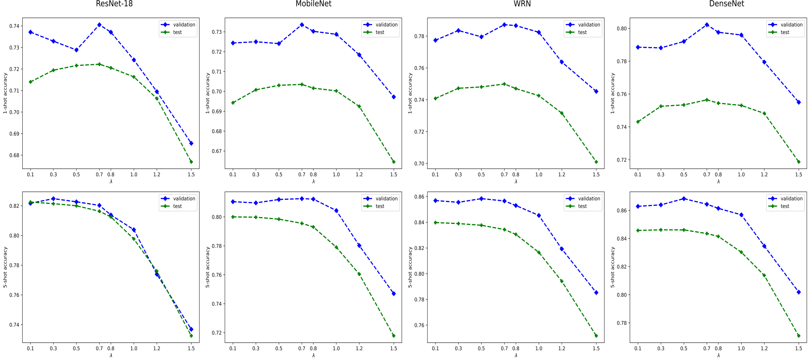
For $\mathbf{W}$, we used the k-nearest neighbor affinities as follows: $w(\mathbf{x}_{q},\mathbf{x}_{p})=1$ if $\mathbf{x}_{p}$ is within the $k$ nearest neighbor of $\mathbf{x}_{q}$, and $w(\mathbf{x}_{q},\mathbf{x}_{p})=0$ otherwise. In our experiments, $k$ is simply chosen from three typical values (3, 5 or 10) tuned over 500 few-shot tasks from the base training classes (i.e., we did not use test data for choosing $k$). We used $k=3$ for miniImageNet, CUB and tieredImageNet and $k=10$ for iNat benchmark. Regularization parameter $\lambda$ is chosen based on the validation class accuracy for miniImageNet, CUB and tieredImageNet. This will be discussed in more details in section 3.6. For the iNat experiments, we simply fix $\lambda=1.0$, as there is no validation set for this benchmark.

We evaluated LaplacianShot over five different benchmarks, with different scenarios and difficulties: Generic image classification, fine-grained image classification, cross-domain adaptation, and imbalanced class distributions. We report the results of LaplacianShot for miniImageNet, tieredImageNet, CUB and iNat datasets, in Tables 1, 2 and 3, along with comparisons with state-of-the-art methods.

Generic image classification: Table 1 reports the results of generic image classification for the standard miniImageNet and tieredImageNet few-shot benchmarks. We can clearly observe that LaplacianShot outperforms state-of-the-art methods by large margins, with gains that are consistent across different settings and network models. It is worth mentioning that, for challenging scenarios, e.g., 1-shot with low-capacity models, LaplacianShot outperforms complex meta-learning methods by more than 9%. For instance, compared to well-known MAML (Finn et al. 2017) and ProtoNet (Snell et al. 2017), and to the recent MetaoptNet (Lee et al. 2019), LaplacianShot brings improvements of nearly 22%, 17%, and 9%, respectively, under the same evaluation conditions. Furthermore, it outperforms the very recent transductive approaches in (Dhillon et al. 2020; Liu et al. 2019a; Liu et al. 2019b) by significant margins. With better learned features with WRN and DenseNet, LaplacianShot brings significant performance boosts, yielding state-of-the art results in few-shot classification, without meta-learning.

Fine-grained image classification: Table 2 reports the results of fine-grained few-shot classification on CUB, with Resnet-18 network. LaplacianShot outperforms the best performing method in this setting by a 7% margin.

Cross-domain (mini-ImageNet $\rightarrow$ CUB): We perform the very interesting few-shot experiment, with a cross-domain scenario, following the setting in (Chen et al. 2019). We used the ResNet-18 model trained on the miniImagenet base classes, while evaluation is performed on CUB few-shot tasks, with 50 test classes. Table 2 (rightmost column) reports the results. In this cross-domain setting, and consistently with the standard settings, LaplacianShot outperforms complex meta-learning methods by substantial margins.

Imbalanced class distribution: Table 3 reports the results for the more challenging, class-imbalanced iNat benchmark, with different numbers of support examples per class and, also, with high visual similarities between the different classes, making class separation difficult. To our knowledge, only (Wertheimer & Hariharan 2019; Wang et al. 2019) report performances on this benchmark, and SimpleShot (Wang et al. 2019) represents the state-of-the-art. We compared with SimpleShot using unnormalized extracted features (UN), L2 and CL2 normalized features. Our Laplacian regularization yields significant improvements, regardless of the network model and feature normalization. However, unlike SimpleShot, our method reaches its best performance with the unnormalized features. Note that, for iNat, we did not use the rectified prototypes. These results clearly highlight the benefit Laplacian regularization brings in challenging class-imbalance scenarios.

Choosing the Value of $\lambda$: In LaplacianShot, we need to choose the value of regularization parameter $\lambda$, which controls the trade-off between the nearest-prototype classifier term ${\mathbf{a}}_{q}$ and Laplacian regularizer ${\mathbf{b}}_{q}^{i}$. We tuned this parameter using the validation classes by sampling $500$ few-shot tasks. LaplacianShot is used in each few-shot task with the following values of $\lambda$: $[0.1,0.3,0.5,0.7,0.8,1.0,1.2,1.5]$. The best $\lambda$ corresponding to the best average 1-shot and 5-shot accuracy over validation classes/data is selected for inference over the test classes/data. To examine experimentally whether the chosen values of $\lambda$ based on the best validation accuracies correspond to good accuracies in the test classes, we plotted both the validation and test class accuracies vs. different values of $\lambda$ for miniImageNet (Figure 1). The results are intuitive, with a consistent trend in both 1-shot and 5-shot settings. Particularly, for 1-shot tasks, $\lambda=0.7$ provides the best results in both validation and test accuracies. In 5-shot tasks, the best test results are obtained mostly with $\lambda=0.1$, while the best validation accuracies were reached with higher values of $\lambda$. Nevertheless, we report the results of LaplacianShot with the values of $\lambda$ chosen based on the best validation accuracies.

Effects of Laplacian regularization: We conducted an ablation study on the effect of each term in our model, i.e., nearest-prototype classifier $\mathcal{N}(\mathbf{Y})$ and Laplacian regularizer $\mathcal{L}(\mathbf{Y})$. We also examined the effect of using prototype rectification, i.e., $\tilde{{\mathbf{m}}}_{c}$ instead of ${\mathbf{m}}_{c}$. Table 4 reports the results, using the ResNet-18 network. The first row corresponds to the prediction of the nearest neighbor classifier ($\lambda=0$), and the second shows the effect of adding Laplacian regularization. In the 1-shot case, the latter boosts the performances by at least 3%. Prototype rectification (third and fourth rows) also boosts the performances. Again, in this case, the improvement that the Laplacian term brings is significant, particularly in the 1-shot case (2 to 3%).

Convergence of transductive LaplacianShot inference: The proposed algorithm belongs to the family of bound optimizers or MM algorithms. In fact, the MM principle can be viewed as a generalization of expectation-maximization (EM). Therefore, in general, MM algorithms inherit the monotonicity and convergence properties of EM algorithms (Vaida 2005), which are well-studied in the literature. In fact, Theorem 3 in (Vaida 2005) states a simple condition for convergence of the general MM procedure, which is almost always satisfied in practice: The surrogate function has a unique global minimum. In Fig. 2, we plotted surrogates $\mathcal{B}_{i}(\mathbf{Y})$, up to a constant, i.e., Eq. (7), as functions of the iteration numbers, for different networks. One can see that the value of $\mathcal{B}_{i}(\mathbf{Y})$ decreases monotonically at each iteration, and converges, typically, within less than 15 iterations.

Inference time: We computed the average inference time required for each 5-shot task. Table 5 reports these inference times for miniImageNet with the WRN network. The purpose of this is to check whether there exist a significant computational overhead added by our Laplacian-regularized transductive inference, in comparison to inductive inference. Note that the computational complexity of the proposed inference is $\mathcal{O}(NkC)$ for a few-shot task, where $k$ is the neighborhood size for affinity matrix $\mathbf{W}$. The inference time per few-shot task for LaplacianShot is close to inductive SimpleShot run-time (LaplacianShot is only 1-order of magnitude slower), and is 3-order-of-magnitude faster than the transductive fine-tuning in (Dhillon et al. 2020).

References

- Belkin et al. (2006) Belkin, M., Niyogi, P., and Sindhwani, V. Manifold regularization: A geometric framework for learning from labeled and unlabeled examples. Journal of Machine Learning Research, 7:2399–2434, 2006.
- Chen et al. (2019) Chen, W.-Y., Liu, Y.-C., Kira, Z., Wang, Y.-C. F., and Huang, J.-B. A closer look at few-shot classification. In International Conference on Learning Representations (ICLR), 2019.
- Dhillon et al. (2020) Dhillon, G. S., Chaudhari, P., Ravichandran, A., and Soatto, S. A baseline for few-shot image classification. In International Conference on Learning Representations (ICLR), 2020.
- Fei-Fei et al. (2006) Fei-Fei, L., Fergus, R., and Perona, P. One-shot learning of object categories. IEEE Transactions on Pattern Analysis and Machine Intelligence, 28:594–611, 2006.
- Finn et al. (2017) Finn, C., Abbeel, P., and Levine, S. Model-agnostic meta-learning for fast adaptation of deep networks. In International Conference on Machine Learning (ICML), 2017.
- Gidaris & Komodakis (2018) Gidaris, S. and Komodakis, N. Dynamic few-shot visual learning without forgetting. In Conference on Computer Vision and Pattern Recognition (CVPR), 2018.
- Gidaris et al. (2019) Gidaris, S., Bursuc, A., Komodakis, N., Pérez, P., and Cord, M. Boosting few-shot visual learning with self-supervision. In International Conference on Computer Vision (ICCV), 2019.
- He et al. (2016) He, K., Zhang, X., Ren, S., and Sun, J. Deep residual learning for image recognition. In Conference on Computer Vision and Pattern Recognition (CVPR), 2016.
- Hou et al. (2019) Hou, R., Chang, H., Bingpeng, M., Shan, S., and Chen, X. Cross attention network for few-shot classification. In Neural Information Processing Systems (NeurIPS), 2019.
- Howard et al. (2017) Howard, A. G., Zhu, M., Chen, B., Kalenichenko, D., Wang, W., Weyand, T., Andreetto, M., and Adam, H. Mobilenets: Efficient convolutional neural networks for mobile vision applications. Preprint arXiv:1704.04861, 2017.
- Hu et al. (2020) Hu, S. X., Moreno, P. G., Xiao, Y., Shen, X., Obozinski, G., Lawrence, N. D., and Damianou, A. Empirical bayes transductive meta-learning with synthetic gradients. In International Conference on Learning Representations (ICLR), 2020.
- Huang et al. (2017) Huang, G., Liu, Z., Van Der Maaten, L., and Weinberger, K. Q. Densely connected convolutional networks. In Conference on Computer Vision and Pattern Recognition (CVPR), 2017.
- Jiang et al. (2019) Jiang, X., Havaei, M., Varno, F., Chartrand, G., Chapados, N., and Matwin, S. Learning to learn with conditional class dependencies. In International Conference on Learning Representations (ICLR), 2019.
- Kim et al. (2019) Kim, J., Kim, T., Kim, S., and Yoo, C. D. Edge-labeling graph neural network for few-shot learning. In Conference on Computer Vision and Pattern Recognition (CVPR), 2019.
- Lange et al. (2000) Lange, K., Hunter, D. R., and Yang, I. Optimization transfer using surrogate objective functions. Journal of computational and graphical statistics, 9(1):1–20, 2000.
- Lee et al. (2019) Lee, K., Maji, S., Ravichandran, A., and Soatto, S. Meta-learning with differentiable convex optimization. In Conference on Computer Vision and Pattern Recognition (CVPR), 2019.
- Liu et al. (2019a) Liu, J., Song, L., and Qin, Y. Prototype rectification for few-shot learning. Preprint arXiv:1911.10713, 2019a.
- Liu et al. (2019b) Liu, Y., Lee, J., Park, M., Kim, S., Yang, E., Hwang, S., and Yang, Y. Learning to propagate labels: Transductive propagation network for few-shot learning. In International Conference on Learning Representations (ICLR), 2019b.
- Miller et al. (2000) Miller, E., Matsakis, N., and Viola, P. Learning from one example through shared densities on transforms. Conference on Computer Vision and Pattern Recognition (CVPR), 2000.
- Mishra et al. (2018) Mishra, N., Rohaninejad, M., Chen, X., and Abbeel, P. A simple neural attentive meta-learner. In International Conference on Learning Representations (ICLR), 2018.
- Munkhdalai et al. (2018) Munkhdalai, T., Yuan, X., Mehri, S., and Trischler, A. Rapid adaptation with conditionally shifted neurons. In International Conference on Machine Learning (ICML), 2018.
- Narasimhan & Bilmes (2005) Narasimhan, M. and Bilmes, J. A submodular-supermodular procedure with applications to discriminative structure learning. In Conference on Uncertainty in Artificial Intelligence (UAI), 2005.
- Oreshkin et al. (2018) Oreshkin, B., López, P. R., and Lacoste, A. Tadam: Task dependent adaptive metric for improved few-shot learning. In Neural Information Processing Systems (NeurIPS), 2018.
- Qiao et al. (2019) Qiao, L., Shi, Y., Li, J., Wang, Y., Huang, T., and Tian, Y. Transductive episodic-wise adaptive metric for few-shot learning. In International Conference on Computer Vision (ICCV), 2019.
- Qiao et al. (2018) Qiao, S., Liu, C., Shen, W., and Yuille, A. L. Few-shot image recognition by predicting parameters from activations. In Conference on Computer Vision and Pattern Recognition (CVPR), 2018.
- Ravi & Larochelle (2017) Ravi, S. and Larochelle, H. Optimization as a model for few-shot learning. In International Conference on Learning Representations (ICLR), 2017.
- Ren et al. (2018) Ren, M., Triantafillou, E., Ravi, S., Snell, J., Swersky, K., Tenenbaum, J. B., Larochelle, H., and Zemel, R. S. Meta-learning for semi-supervised few-shot classification. In International Conference on Learning Representations ICLR, 2018.
- Russakovsky et al. (2015) Russakovsky, O., Deng, J., Su, H., Krause, J., Satheesh, S., Ma, S., Huang, Z., Karpathy, A., Khosla, A., Bernstein, M., Berg, A. C., and Fei-Fei, L. ImageNet Large Scale Visual Recognition Challenge. International Journal of Computer Vision (IJCV), 115(3):211–252, 2015.
- Rusu et al. (2019) Rusu, A. A., Rao, D., Sygnowski, J., Vinyals, O., Pascanu, R., Osindero, S., and Hadsell, R. Meta-learning with latent embedding optimization. In International Conference on Learning Representations (ICLR), 2019.
- Shi & Malik (2000) Shi, J. and Malik, J. Normalized cuts and image segmentation. IEEE Transactions on Pattern Analysis and Machine Intelligence, 22(8):888–905, 2000.
- Snell et al. (2017) Snell, J., Swersky, K., and Zemel, R. Prototypical networks for few-shot learning. In Neural Information Processing Systems (NeurIPS), 2017.
- Sun et al. (2019) Sun, Q., Liu, Y., Chua, T., and Schiele, B. Meta-transfer learning for few-shot learning. In Conference on Computer Vision and Pattern Recognition (CVPR), June 2019.
- Sung et al. (2018) Sung, F., Yang, Y., Zhang, L., Xiang, T., Torr, P. H., and Hospedales, T. M. Learning to compare: Relation network for few-shot learning. In Conference on Computer Vision and Pattern Recognition (CVPR), 2018.
- Szegedy et al. (2016) Szegedy, C., Vanhoucke, V., Ioffe, S., Shlens, J., and Wojna, Z. Rethinking the inception architecture for computer vision. In Conference on Computer Vision and Pattern Recognition, 2016.
- Tian et al. (2014) Tian, F., Gao, B., Cui, Q., Chen, E., and Liu, T.-Y. Learning deep representations for graph clustering. In AAAI Conference on Artificial Intelligence, 2014.
- Vaida (2005) Vaida, F. Parameter convergence for em and mm algorithms. Statistica Sinica, 15:831–840, 2005.
- Vaswani et al. (2017) Vaswani, A., Shazeer, N., Parmar, N., Uszkoreit, J., Jones, L., Gomez, A. N., Kaiser, u., and Polosukhin, I. Attention is all you need. In Neural Information Processing Systems (NeurIPS), 2017.
- Vinyals et al. (2016) Vinyals, O., Blundell, C., Lillicrap, T. P., Kavukcuoglu, K., and Wierstra, D. Matching networks for one shot learning. In Neural Information Processing Systems (NeurIPS), 2016.
- Von Luxburg (2007) Von Luxburg, U. A tutorial on spectral clustering. Statistics and computing, 17(4):395–416, 2007.
- Wah et al. (2011) Wah, C., Branson, S., Welinder, P., Perona, P., and Belongie, S. The caltech-ucsd birds-200-2011 dataset. 2011.
- Wang & Carreira-Perpinán (2014) Wang, W. and Carreira-Perpinán, M. A. The laplacian k-modes algorithm for clustering. Preprint arXiv:1406.3895, 2014.
- Wang et al. (2019) Wang, Y., Chao, W.-L., Weinberger, K. Q., and van der Maaten, L. Simpleshot: Revisiting nearest-neighbor classification for few-shot learning. Preprint arXiv:1911.04623, 2019.
- Wertheimer & Hariharan (2019) Wertheimer, D. and Hariharan, B. Few-shot learning with localization in realistic settings. In Conference on Computer Vision and Pattern Recognition (CVPR), 2019.
- Weston et al. (2012) Weston, J., Ratle, F., Mobahi, H., and Collobert, R. Deep learning via semi-supervised embedding. In Neural networks: Tricks of the trade, pp. 639–655. Springer, 2012.
- Ye et al. (2020) Ye, H.-J., Hu, H., Zhan, D.-C., and Sha, F. Few-shot learning via embedding adaptation with set-to-set functions. In Conference on Computer Vision and Pattern Recognition (CVPR), 2020.
- Yuan et al. (2017) Yuan, J., Yin, K., Bai, Y., Feng, X., and Tai, X. Bregman-proximal augmented lagrangian approach to multiphase image segmentation. In Scale Space and Variational Methods in Computer Vision (SSVM), 2017.
- Yuille & Rangarajan (2001) Yuille, A. L. and Rangarajan, A. The concave-convex procedure (CCCP). In Neural Information Processing Systems (NeurIPS), 2001.
- Zagoruyko & Komodakis (2016) Zagoruyko, S. and Komodakis, N. Wide residual networks. In British Machine Vision Conference (BMVC), 2016.
- Zhang et al. (2019) Zhang, J., Zhao, C., Ni, B., Xu, M., and Yang, X. Variational few-shot learning. In International Conference on Computer Vision (ICCV), 2019.
- Zhang et al. (2007) Zhang, Z., Kwok, J. T., and Yeung, D.-Y. Surrogate maximization/minimization algorithms and extensions. Machine Learning, 69:1–33, 2007.
- Zhou et al. (2004) Zhou, D., Bousquet, O., Lal, T. N., Weston, J., and Schölkopf, B. Learning with local and global consistency. In Neural Information Processing Systems (NeurIPS), 2004.
- Ziko et al. (2018) Ziko, I., Granger, E., and Ben Ayed, I. Scalable laplacian k-modes. In Neural Information Processing Systems (NeurIPS), 2018.