CMacIonize 2.0: a novel task-based approach to
Monte Carlo
radiation transfer
Abstract
Context. Monte Carlo radiative transfer (MCRT) is a widely used technique to model the interaction between radiation and a medium, and plays an important role in astrophysical modelling and when comparing those models with observations.
Aims. In this work, we present a novel approach to MCRT that addresses the challenging memory access patterns of traditional MCRT algorithms, which hinder optimal performance of MCRT simulations on modern hardware with a complex memory architecture.
Methods. We reformulate the MCRT photon packet life cycle as a task-based algorithm, whereby the computation is broken down into small tasks that are executed concurrently. Photon packets are stored in intermediate buffers, and tasks propagate photon packets through small parts of the computational domain, moving them from one buffer to another in the process.
Results. Using the implementation of the new algorithm in the photoionization MCRT code CMacIonize 2.0, we show that the decomposition of the MCRT grid into small parts leads to a significant performance gain during the photon packet propagation phase, which constitutes the bulk of an MCRT algorithm, as a result of better usage of memory caches. Our new algorithm is a factor 2 to 4 faster than an equivalent traditional algorithm and shows good strong scaling up to 30 threads. We briefly discuss how our new algorithm could be adjusted or extended to other astrophysical MCRT applications.
Conclusions. We show that optimising the memory access patterns of a memory-bound algorithm such as MCRT can yield significant performance gains.
Key Words.
Methods: numerical – radiative transfer1 Introduction
In the mid 2000s, the clock speed of a single CPU core reached its limits, imposed by the physics of heat dissipation in increasingly smaller and denser circuits. Since then, increased CPU performance has been delivered by increased parallelism rather than a raw increase in speed. Scientific progress through increased performance started to crucially depend on scalability, a concept that was relatively unimportant in astrophysical computing until then. The impact on Monte Carlo radiative transfer simulations can be seen by comparing historical works. While Price 1969 mentions a reference speed of photon packets in 200 minutes for an 18 cell grid, Wood et al. 2004 quote a speed of photon packets per minute for a similar algorithm on a grid, or a speedup of roughly . CMacIonize 1.0, a rewrite of the Wood et al. 2004 code manages photon packets per minute for a grid on a single CPU core, or a speed up of less than 10, well below the expected factor of if Moore’s law for single CPUs would still hold. This factor can be recovered by running CMacIonize 1.0 on cores, a representative number for a modern computing node.
While the speed of CPUs increased and ultimately hit a limit, memory went from being a limiting factor (Price 1969 mentions that a 20 cell grid was impractical, presumably for this reason) over being abundant to being a limiting factor again. Modern computers support memory sizes of and with that grid sizes of up to cells (every double-precision floating point number stored in a cell of a cell grid corresponds to 8 GB of memory space required). This memory, however, is generally laid out in a complex way, with most of the memory having a relatively low bandwidth. This results in algorithms that are severely memory-bound, i.e. the speed of the algorithm is dominated by the memory bandwidth rather than the clock speed of the CPU cores. The speed of these algorithms crucially depends on memory access patterns that can lead to efficient cache usage, concepts that are still relatively new in astrophysical computing.
These two factors (increased parallelism and increased memory boundedness) have made it increasingly hard to develop astrophysical software in the last decade. Successful algorithms have required a radical redesign, often depending on an active involvement of computer scientists in the development process (Bordner & Norman 2012; Gonnet et al. 2013; Schaller et al. 2016; White et al. 2016; Nordlund et al. 2018; Borrow et al. 2018). Given the current trends in hardware technology, this way of developing astrophysical software may become the norm.
In this work, we present a novel approach to the algorithmic framework of the Monte Carlo radiative transfer (MCRT) technique, which is used for radiation transport simulations in various fields, including, for example, photoionization (Hubber et al. 2016; Vandenbroucke et al. 2018), dust continuum radiation (Steinacker et al. 2013; Camps & Baes 2020), resonant line transfer (Smith et al. 2015; Behrens et al. 2018) and particle physics (X-5 Monte Carlo Team 2003; Agostinelli et al. 2003). We reformulate the photon packet propagation mechanism at the heart of the MCRT technique as a task-based algorithm. The algorithm is defined in terms of individual units of computational work, each involving small amounts of memory and with clear inter-dependencies governing which tasks can be executed at what time and which tasks can be executed concurrently.
The major bottleneck in contemporary MCRT algorithms is the grid structure used to discretize the interstellar medium in space. In multi-node, distributed memory setups, it is easily understood that this grid structure leads to significant overheads, either because the entire structure needs to be duplicated on all nodes (Vandenbroucke & Wood 2018; Camps & Baes 2020), or because photon packets need to be communicated between nodes (Harries et al. 2019). On shared memory systems, the grid is, however, a bottleneck as well, this time due to bandwidth issues. The grid occupies a large (possibly continuous) chunk of memory that is accessed concurrently by different threads. Due to the random nature of the MCRT algorithm, these concurrent access events happen in an arbitrary fashion that puts significant strains on the memory bandwidth, suffers from generally unpredictable retrieval delays and makes it nearly impossible for algorithm implementations to efficiently use fast memory caches.
The obvious solution to these issues is to give up on the idea of a single monolithic grid structure, even in the case of a shared memory algorithm, and instead decompose the grid into many smaller parts, which we will call subgrids. These subgrids can then act as the small memory resources on which the tasks in the task-based algorithm operate. As in the case of a distributed-memory grid, this inevitably means storing photon packets that transition from one such subgrid to a neighbouring subgrid, which requires the use of buffers (Harries et al. 2019).
Any minimal task-based MCRT algorithm hence depends on three crucial ingredients: an efficient strategy to decompose the computational grid into independent subgrids, the formulation of a set of tasks that perform photon packet propagation based on interactions between these subgrids and the corresponding buffers, and an algorithm to create and schedule these tasks. At the same time, the task-based approach does not require any changes to the implementation of the physical equations governing the simulation. The interaction between the photon packets and the medium represented by each of the cells in the individual subgrids can still be computed in the same way as for a single grid structure. What needs to change is the idea of a monolithic photon packet life cycle, whereby a photon packet is tracked sequentially from its generation at a source location, throughout its propagation through the grid structure, until it is terminated by an absorption event or because it leaves the computational domain. An example of this basic life cycle is depicted in Fig. 1. In the new task-based algorithm, photon packet generation and propagation, as well as optional additional processes like scattering and re-emission, are treated separately and not necessarily consecutively.
We introduce the task-based algorithm in Sect. 2 using the specific example of photoionization as it is implemented in CMacIonize 2.011 1 The source code of CMacIonize 2.0 is hosted on https://github.com/bwvdnbro/CMacIonize, the new version of the code presented in Vandenbroucke & Wood 2018. This allows us to focus on the basics of the task-based algorithm, without the need to expand into extra complexities. For the same reason, we assume a regular grid structure that is subdivided into regular subgrids with identical dimensions, and we limit the discussion to one or more point sources. In Sect. 3 we validate this task-based algorithm, and in Sect. 4 we compare its performance with that of a more conventional MCRT photoionization algorithm, i.e. CMacIonize 1.0. We also discuss practical aspects such as the memory requirements of the algorithm and its various components. Possible extensions of the algorithm are discussed in Sect. 5. We highlight some features of CMacIonize 2.0 that go beyond the basic task-based algorithm, and discuss how the task-based algorithm could be extended for other MCRT applications. In Sect. 6, we end with a summary and some overall conclusions.
2 Task-based algorithm
2.1 Calculating photoionization
The aim of the photoionization algorithm is to determine the equilibrium temperature and ionization state of an interstellar medium that is exposed to a radiation field with a known ionizing spectrum. Depending on the chemical elements that are included and the cooling and heating processes that are considered, this problem can be arbitrarily complex. We here describe the example of a hydrogen-only gas, which captures all the essential aspects of the algorithm.
Within each cell of the computational domain, the composition of the hydrogen plasma is characterised by two variables: the hydrogen number density, which is assumed to remain constant during the simulation, and the neutral hydrogen fraction, which encodes the ionization state of the medium within the cell. The latter is computed by balancing the number of ionization events per unit time, caused by the absorption of ionizing radiation, with the collisional recombination rate, which depends on the electron temperature and the free electron density. The temperature, in turn, can be computed by balancing the photoionization heating rate with an appropriate cooling rate. If the characteristics of the embedding photoionizing radiation field are known, one can self-consistently solve for both the neutral fraction (and electron density) and the temperature.
To model the interaction between the radiation field and the medium in each cell, the radiation is discretized using a (large) number of photon packets. Each photon packet carries a fixed photoionization rate, and is emitted in a randomly sampled direction and with a randomly sampled frequency, which determines its photoionization cross section. Both random values are sampled from appropriate distribution functions; emission is usually assumed isotropic, while frequencies are distributed according to a source spectrum.
The photon packets are propagated through the grid until a randomly sampled optical depth is reached (distributed exponentially). The optical depth along the path is computed from the path lengths traversed by the photon packet in each cell, using the neutral hydrogen density in each cell and the photoionization cross section of the photon packet. These same path lengths and cross sections are also accumulated in each cell for each passing photon packet, providing an estimate of the absorbed ionizing radiation field.
When a photon packet reaches its target optical depth, it is absorbed, i.e. it is assumed that all physical photons in the packet have been absorbed along the way. At this point, the photon packet is reused to sample the diffuse radiation field caused by ionizing recombinations. For a solar-metallicity Hii region with a temperature of K, of the photons emitted by recombination events have frequencies above the ionization threshold of hydrogen and will contribute to the ionizing radiation field. A corresponding fraction of the absorbed photon packets is therefore re-emitted in a randomly sampled new direction and with a randomly sampled new frequency. Since in our algorithm this re-emission happens instantaneously, it is essentially treated as a scattering event.
At the end of the photon packet propagation phase, each cell holds an estimate of the absorbed ionizing radiation field, which is then used to compute the temperature and neutral fraction in the cell. Since the neutral fraction determines the neutral hydrogen density, which in turn sets the opacity of the cell for ionizing radiation, the whole process must be repeated until a converged solution is obtained. Starting from a highly ionized medium that is transparent for ionizing radiation, convergence is typically reached within 10 iterations (Vandenbroucke & Wood 2018). Convergence is much slower when starting from an assumed neutral initial medium.
2.2 Tasks
Within our task-based photoionization algorithm, the conventional photon packet life cycle is broken up as follows (see Fig. 1):
- •
Photon packet generation: a number of photon packets is generated sequentially from the source model and placed in an input buffer for the subgrid containing the source location. This buffer is then flagged for processing, while the thread that executed this work moves on to do something else.
- •
Photon packet propagation: the photon packets in a subgrid’s input buffer are propagated through the subgrid, and are placed in buffers according to their interaction with that subgrid (see Fig. 2). Photon packets that leave the subgrid through one of its boundaries are passed on to buffers for neighbouring subgrids, while photon packets that are absorbed internally are tracked in another buffer. Photon packets that leave the subgrid through a boundary that is also a simulation box boundary are terminated. During this step, the path length counters in the cells that keep track of the ionizing radiation field are updated.
- •
Photon packet re-emission: photon packets that were put in a subgrid buffer after absorption are re-emitted according to the local properties of the relevant subgrid cell. In practice, this means that the properties (energy, propagation direction) of the photon packets are updated inside the buffer. Photon packets that are not eligible for re-emission are terminated and removed from the buffer.
Any of these steps can be executed concurrently by different threads, as long as causality is respected for individual photon packets. Each step represents a task: a small amount of computational work with a clearly defined memory footprint and known dependencies. The efficient scheduling and execution of these tasks is at the core of the task-based algorithm. All tasks are typically put into one or more queues. Parallel execution threads query those queues for available tasks and execute them, until all tasks have been executed. Tasks are added to the queues by a scheduler that makes sure causality for tasks is respected (Gonnet et al. 2016). By using a separate queue for each thread, it is possible to sort tasks so that threads preferentially execute tasks accessing the same data structures to help increase cache efficiency.
In conventional task-based algorithms, the tasks and their inter-dependencies are known at the start of the calculation (Gonnet et al. 2016). In our task-based MCRT algorithm, however, the set of tasks is not a priori known because of the random nature of the algorithm. When a task finishes, it can create a new task. This leads to the following implicit task dependencies:
- •
An initial setup loop creates photon packet generation tasks for all sources in the model.
- •
A photon packet generation task creates a single photon packet propagation task that acts on the buffer that was filled by the generation task and on the subgrid that contains the position of the point source that emitted the photons.
- •
A photon packet propagation task creates new propagation tasks and up to one re-emission task when the respective buffers containing the outgoing photon packets are full. These new tasks act on the corresponding output buffers and the subgrid associated with it: the corresponding neighbouring subgrid for neighbour buffers, and the original subgrid for the internal output buffer.
- •
A photon packet re-emission task similarly creates up to one propagation task.
2.3 Subgrids and photon packet buffers
The spatial grid in our algorithm is stored as an array of pointers to individual subgrid structures that are completely self-contained. Each subgrid stores the geometry of its cells plus all of the physical quantities and variables for these cells. For a regular grid, the cell geometry can be represented by just the anchor point and the side lengths of the cuboid that encompasses the subgrid. Furthermore, a subgrid also stores information about its position within the larger grid, i.e. it stores the indices of the neighbouring subgrids in the array. This is illustrated with arrows in the left panel of Fig. 2.
Most of the MCRT algorithm is implemented as functions that directly manipulate an individual subgrid. The photon propagation step takes an input buffer, propagates all the photon packets it contains through the subgrid, and stores the resulting outgoing photon packets in appropriate output buffers. The re-emission step uses local cell variables to decide if and how to re-emit a photon packet that was locally absorbed earlier. These parts of the algorithm are almost identical to the corresponding parts in a non task-based version of the algorithm.
Each buffer contains a fixed number of photon packet slots and a counter indicating the actual number of photon packets currently stored in the buffer. It also stores general directional information about the photon packets in the buffer that is used to speed up the continued propagation in other subgrids. For example, if the buffer collects photon packets that leave through the front face of the subgrid cuboid, then these photon packets will all enter the neighbouring subgrid through the back face.
Each photon packet stores all the information required to propagate the packet through the grid. This includes the propagation direction, the current position, the optical depth accumulated so far, the target optical depth, and the energy/frequency and/or interaction cross sections required in the optical depth calculation. The idea is that the propagation of a photon packet can be paused at any time during its life cycle.
The task scheduler provides a pool of pre-allocated photon packet buffers that are assigned and reassigned as needed during the operation of the algorithm. Specifically, each subgrid is assigned an output buffer corresponding to each of its neighbouring subgrids in addition to a single re-emission buffer. Furthermore, every source is assigned an output buffer as well. In each case, whenever a task fills up or otherwise completes an output buffer, the buffer is passed on to the scheduler to serve as an input buffer for another task, and a new empty buffer is acquired to replace the original output buffer.
2.4 Queues and scheduling
The task scheduler manages a number of queues to track tasks that are ready to be executed. The information required to execute a particular task is stored in a small data structure including the type of the task and the indices of the resources involved in its execution. For example, a photon propagation task references the relevant subgrid and input photon buffer.
Our algorithm uses several queues. Each execution thread is assigned a per-thread queue that stores the propagation tasks for the subgrids that are often accessed by that specific thread and from which that thread preferentially gets its tasks. Moreover, there is a single shared queue that stores the photon packet generation and re-emission tasks that are only executed if no propagation tasks are available.
As illustrated in Fig. 3, during the task execution loop, a thread
- 1.
queries its own queue for a propagation task and executes it, or, if this fails,
- 2.
tries to steal a propagation task from another thread’s queue and executes it, or, if this fails,
- 3.
tries to acquire a re-emission or photon generation task from the shared queue and executes it, or, if this fails,
- 4.
tries to prematurely schedule a non-full outgoing photon buffer for one of the subgrids.
The order of these actions has been carefully chosen to maximise the throughput of photon packets, since this minimises the number of buffers required to store photon packets that have not yet been terminated. The last action in the above list is necessary to guarantee that the algorithm will finish. Indeed, output buffers associated with individual subgrids will not necessarily be full by the time all photon packets have been injected into the grid, so that an alternative method is required to ensure that packets in partially filled buffers are properly processed.
Because the shared queue contains all photon packet generation tasks, buffers can only be prematurely scheduled once all photon packets have been generated. Even then, care must be taken not to reduce the efficiency of the algorithm by prematurely scheduling too many partially filled photon packet buffers when the photon packet propagation phase is winding down. This is achieved by preferentially scheduling buffers with a larger number of photon packets as long as they are available.
If a thread cannot obtain an executable task after performing all of the actions in the above list, then there is a possibility that all photon packets have been successfully propagated through the grid, and an appropriate check is performed to detect this. If this check fails, the thread repeats the scheme above in case a new or existing task has become eligible for execution. The loop continues until the thread detects a successful termination of the propagation phase. At this point all threads will agree that the propagation phase finished and will exit the parallel environment.
After the propagation phase finishes, additional subgrid tasks can be executed, such as the calculation of the ionization balance in each cell. Generally, these tasks can again be performed in parallel. When appropriate, the photon propagation and cell update phases are repeated until convergence has been reached. The exit condition for each phase inevitably introduces a synchronisation point within the parallel execution where load imbalances lead to idle time for some of the threads. However, as long as the number of phase iterations is small compared to the number of tasks performed within each phase, the total load imbalance should be small.
2.5 Subgrid copies
An important feature of our algorithm is the ability to duplicate subgrids for which there is a high contention. In many simulated models, some subgrids have a significantly higher-than-average computational load. A good example is a model with a single point source of radiation. In such a simulation, the subgrid containing the source position will receive all of the initial photon packet propagation tasks. Since each photon packet propagation task needs unique access to this subgrid, this leads to a very strong bottleneck early in the simulation.
This problem can be addressed by making one or more copies of the subgrids for which a lot of contention is expected. These copies are added to the list of subgrids as independent subgrids, but inherit the positions and optical properties of their parent subgrid. The neighbouring relations between the original subgrid, its neighbours, and the copies are rearranged so that each subgrid still has an outgoing neighbour on all sides (see Fig. 4). Specifically, each of the neighbouring subgrids stores an outgoing link to just one of the subgrid copies, distributed evenly over the copies to help balance their workload. Each subgrid copy keeps track of its own radiation field counters and behaves as if it was not related to its parent. At the end of the photon propagation phase, the counters for all copies are accumulated into the parent counters and all copies are discarded.
If the individual subgrids are sufficiently small, the copy procedure incurs little overhead, while significantly improving the load balancing of the algorithm. However, a successful duplication strategy requires a good prediction of the computational load of each subgrid. One might obtain such an estimate based on a previous simulation run or iteration or based on a low resolution bootstrap simulation. While these options could in principle provide an accurate prediction, they are often impractical. We found that a heuristic approach is easier to use and provides a sufficiently accurate estimate for our purposes.
The heuristic we chose to adopt assumes that there is a strong correlation between the presence of a source within a subgrid and an increased load within that subgrid and its neighbours. Each subgrid is assigned a copy level, where a copy level equal to gives rise to duplicates (including the original). The user specifies a single parameter, , indicating the copy level for subgrids that contain a source position. Once this maximum copy level has been assigned to all subgrids associated with a source, the heuristic recursively traverses the subgrid structure and ensures that neighbouring subgrids are at most one copy level apart. If a given subgrid has level , then all of its neighbours have levels . This automatically leads to a hierarchical structure of duplicates that captures the expected computational load for a uniform density distribution close to a source (see Fig. 5), and we found that this approach works well in all our tests.
2.6 Memory management and locking
The multiple execution threads of our algorithm operate in a single, shared memory environment. It is therefore necessary to provide the appropriate synchronisation mechanisms for accessing common data structures. A key benefit of the subgrid approach presented in the previous sections is that most of the data are local to the corresponding subgrid. As long as at most a single task operates on a given subgrid at any one time, there is no need to synchronise access to these local data. The data structures that do need synchronised access thus include the subgrids, the photon packet buffers (see Sect. 2.3), the task definitions, and the task queues (see Sect. 2.4). All synchronisation occurs at the level of the task scheduler and never within any of the tasks themselves.
To begin with, each of the queues managed by the task scheduler is protected by a single lock that must be acquired by a thread before it can retrieve a new task from the queue. As described in Sect. 2.4, each thread has its own preferential queue and only occasionally accesses the other queues. As a result, contention on the queue locks is low and the overhead is minimal.
The situation is more complicated for the data structures holding the information describing each task and for the photon packet buffers. Our algorithm continuously creates new tasks and terminates other tasks as the simulation proceeds (see Sect. 2.2). Similarly, photon packet buffers are continuously being assigned and reassigned (see Sect. 2.3). To minimise the overhead of this dynamic process, an array of empty task descriptions and an array of empty photon packet buffers are pre-allocated before parallel task execution begins. The main drawback of this approach is that the arrays have a fixed size and thus must be chosen sufficiently large to support the requirements of the simulation. It is therefore essential to have a good heuristic for predicting these requirements. We will return to this issue in Sect. 4.
Because task descriptions and photon packet buffers are frequently accessed from all execution threads, protecting access with a single, global lock for each array would cause substantial overhead. Instead, each entry in these arrays is equipped with its own lock to allow fine-grained access control. In addition, a single atomic index counter (per array) is used to help locating available entries. Specifically, whenever a thread needs to acquire a new entry, it atomically increments the index counter, computes an actual array index from the counter by taking its value modulo the array size, and then attempts to acquire the lock for the corresponding entry. If this is unsuccessful, the entry is already in use and the whole procedure is repeated. Because entries can be expected to be released in roughly the same order as in which they were acquired, this rolling index mechanism will often be successful after one or just a few attempts.
Lastly, all subgrids in the distributed grid structure, including any duplicates (see Sect. 2.5), are also pre-allocated before parallel task execution begins, and each subgrid is equipped with a lock that controls access to it.
As mentioned in Sect. 2.4, a task description lists the resources needed by the task. For example, a photon propagation task references the relevant subgrid and input photon buffer. Following the technique presented by Gonnet et al. 2016, a thread that wants to acquire a task tries to acquire a lock for all the resources listed by the task. If this does not succeed, any locks that were successfully acquired are released again, and the thread moves on to look for another eligible task. This mechanism ensures exclusive access to a task’s resources during its operation.
3 Validation
We have validated the new photoionization algorithm using a suite of tests and benchmark runs. The parameter- and initial condition files for these tests are part of the public CMacIonize 2.0 repository. Reference results were already presented in Vandenbroucke & Wood 2018 and have not changed, since no changes were made to the physical equations we are solving. Below, we give a brief overview of these tests, the aspects of the code they test, and any changes made since the release of CMacIonize 1.0.
3.1 Strömgren sphere
When a single source with an ionising UV luminosity photoionizes a uniform, hydrogen-only medium with number density and a fixed collisional recombination rate , it will ionize out a sphere with a radius that can be approximated as
| (1) |
If the UV source furthermore emits radiation at a fixed frequency, so that the photoionization cross section can be assumed to be constant, then the ionization balance equation at radius can be written as
| (2) |
with the hydrogen neutral fraction at radius .
This equation can be numerically solved on a grid in to provide a semi-analytic reference solution for a photoionization simulation using the same setup. In addition to testing that the correct volume is ionized out (this diagnostic only depends on the recombination rate), this also checks that the width of the ionization front and the exponential extinction of the ionizing radiation is resolved correctly (these diagnostics also depend on the photoionization cross section).
The Strömgren volume test is an ideal test case for any basic photoionization algorithm, since it tests all important aspects of the algorithm: the interaction between individual photon packets and the medium, the update of the cell properties at the end of each iteration, and the iterative scheme to obtain a converged solution. More specifically for the new MCRT algorithm, this test checks that all photon packets are correctly passed on from one subgrid to another, that the contributions from subgrid copies are correctly taken into account, and that subgrid copies are correctly synchronised.
The benchmark test contained in the repository uses a pc box with a uniform hydrogen-only medium with a density . At the centre of the box is a single photoionizing source with an ionizing luminosity that emits monochromatic radiation at the hydrogen photoionization energy, eV. We assume a constant photoionization cross section and a constant recombination rate , and consider a version without and with diffuse re-emission. For the latter case, we assume that photons that get absorbed have a constant probability, , to be re-emitted as photoionizing photons. In this version of the test, the semi-analytic reference solution is no longer accurate, but the ionized volume still satisfies equation (1), albeit with a different value for the ionizing luminosity, .
We discretize the medium on a cell grid, and perform the photoionization simulation using photon packets for 20 iterations. The results of both versions of the test are shown in Fig. 6 and are statistically equivalent to the results obtained with CMacIonize 1.0 (Vandenbroucke & Wood 2018).
3.2 Lexington Hii region benchmark
In an astrophysical photoionization (or Hii) region, a significant fraction of the UV extinction is due to the photoionization of helium. Furthermore, the photoionization cross sections for hydrogen, helium and other chemical elements depend on the energy of the ionizing photons, and the recombination rates depend on the local electron temperature. The temperature itself is an equilibrium value for which the photoionization heating is balanced by the radiative cooling due to deexcitation of excited states of predominantly metal ions. Some of the radiation released by recombining hydrogen and helium will still be emitted at ionizing frequencies, so that an additional diffuse ionizing field is generated. To properly resolve the structure of these regions, even for the basic case of a uniform medium with a single photoionizing source, it is hence necessary to track more chemical elements and to treat the photoionization cross sections, recombination rates, and temperature self-consistently.
Due to the complexity of this problem, a (semi-)analytic reference solution does not exist. However, a variety of benchmark tests have been formulated in literature, e.g. the Lexington benchmarks (Ferland 1995; Péquignot et al. 2001). These benchmarks consist of a pc uniform box with a spherical cavity with radius pc in the centre. In the centre of this cavity, a single black-body ionizing source is located. The difference between the two versions is the assumed temperature and ionizing luminosity of the source, K and for the low temperature benchmark, and K and for the high temperature benchmark. The hydrogen number density outside the central cavity is set to , and the density of the other elements we consider is given by the relative number abundances: , , , , and . All photoionization cross sections, recombination rates and re-emission probabilities are computed self-consistently using the same atomic data used by Vandenbroucke & Wood 2018 and are not part of the benchmark parameters.
In addition to testing the aspects of the basic photoionization algorithm that are also tested by the Strömgren volume test, this test also tests the handling of diffuse photon packets, and the proper tracking and synchronisation of path length counters for elements other than hydrogen. It also tests the more elaborate temperature and ionization structure calculation at the end of each iteration (an aspect that has not changed from CMacIonize 1.0.
The benchmarks contained in the repository use a grid to discretize the medium, and require photon packets for 20 iterations. The number of photon packets required is significantly higher than in an equivalent Strömgren volume test because of the low flux in the high energy tail of the black-body spectrum, which we need to sample accurately to get accurate ionic fractions for coolants with high ionization energies. photon packets are sufficient to reproduce the average temperature profile, while photon packets are required to get an acceptable noise level for the abundances of individual ions.
Fig. 7 shows the temperature profiles for both versions of the test, as well as a 1D reference solution computed with Cloudy (Ferland et al. 2017), using the same input parameters. We find a reasonable agreement, with some deviations that can be traced back to differences between our physical model and that of Cloudy. Similar observations can be made for the ionic fraction profiles for both versions of the test, as presented in Fig. 8. All results are again statistically equivalent to the results presented in Vandenbroucke & Wood 2018, since nothing changed to our physical model.
3.3 Turbulent boxes
The two tests described above use a uniform medium and are essentially 1D tests because of the spherical symmetry of their setup. This is not representative for real applications, where the density structure and radiation field are truly 3D quantities that cannot be sampled using a 1D method. To validate our new algorithm in a 3D scenario, we need a setup with a range of densities. We can use CMacIonize 1.0 to obtain reference results for the same setup.
As 3D tests, we repeat the Strömgren volume and high temperature Lexington benchmark tests, but this time using a turbulent ISM model as background density field. The turbulent field is generated by running CMacIonize 2.0 in hydrodynamics only mode on a cell grid. Starting from a uniform medium, we drive turbulence using solenoidal forcing in Fourier space, with the method of Alvelius 1999. The simulation is evolved until the probability distribution function and power spectrum of the density and velocity fields reach a steady state. The box size and average density in the box are set to the same values as for the original test. Once the initial condition has been generated, the source is again put in the centre of the box. This time, we do not cut out a pc sphere for our alternative Lexington tests. Detailed results of these turbulent box simulations are described elsewhere (Sartorio & Vandenbroucke, in prep.).

Fig. 9 shows the ionization structure of the turbulent Strömgren volume test, after 10 iterations using photon packets. The density grid produced by the hydro simulation was resampled onto a grid to reduce the computational cost for this test. The ionizing source is located close to an intermediate density filament and ionizes a highly non-symmetric Strömgren volume, predominantly in the directions perpendicular to the filament. The densities of the cells along the individual photon paths span three orders of magnitude. The results for CMacIonize 1.0 and CMacIonize 2.0 are indistinguishable. This can also be seen from the total ionized mass within the box: the old algorithm yields , while the new algorithm gives , consistent with Monte Carlo noise. Both these values are significantly lower than the for a uniform medium, since the recombination rate is dominated by recombination in the filaments that is significantly higher than in the uniform case.


Fig. 10 shows the hydrogen and helium neutral fraction for the turbulent Lexington test. This test uses the same grid structure as the equivalent Strömgren test, and uses photon packets for 20 iterations. As in the uniform Lexington test, the ionization fraction of helium is lower than that of hydrogen but follows the same general trend. The regions where hydrogen and helium are ionized almost have the same size, because the transition from ionized to neutral happens over a short distance near the denser filaments. The top panels of Fig. 10 also show the hydrogen ionization front from the equivalent Strömgren test for comparison. While in principle both tests should yield the same ionized region, the simplified physics treatment and the absence of a diffuse field in the Strömgren test lead to small differences in the geometry of the Hii region.
Fig. 11 and Fig. 12 show the temperature and ionic fractions for the turbulent Lexington test. The general trends are the same as for the equivalent uniform test, shown in Fig. 7 and Fig. 8. The temperature is relatively constant and in the range K throughout most of the Hii region, and then steeply rises towards a temperature of K and more near the ionization front. The central parts of the Hii region are dominated by ions with high ionization energies, while ions with lower ionization energies start to dominate closer to the ionization front as absorption depletes high energy photons. Of significant interest are the regions that are not directly exposed to the star and hence can only have been ionized by diffuse radiation. One such region can clearly be identified to the right of the ionizing source in the slices. This region is characterised by a relatively low temperature and dominated by , , , and .
3.4 Other tests
The tests above verify all aspects of the new MCRT algorithm. CMacIonize 2.0 has additional capabilities, such as the possibility to run radiation hydrodynamics simulations (see Sect. 5.4), and these also have dedicated tests. We mention them here for completeness.
The coupling between photoionization and hydrodynamics is realised by assuming a two-temperature approximation, whereby hydrodynamical integration time steps are alternated with photoionization steps, and the hydrodynamic pressure is updated according to the ionization state returned by the MCRT algorithm. Neutral gas is set to a chosen low temperature, and ionized gas to a chosen high temperature. The temperature for cells that are partially ionized is obtained by linearly interpolating between these two temperatures. This approach is identical to that used by Bisbas et al. 2015, and is tested using their starbench benchmark test that models the early expansion of a D-type ionization front. Results are consistent with Vandenbroucke & Wood 2018.
Sartorio et al. 2019 extended the algorithm to also include the gravitational potential of a point source, in order to model trapped Hii regions surrounding massive protostars. To validate the coupling between hydrodynamics and the external potential, we created a new steady-state accretion flow test, similar to Vandenbroucke et al. 2019. This so-called Bondi test starts with a uniform medium and uses inflow boundary conditions that are consistent with the analytic Bondi profile for the assumed point mass potential at the radius of the boundaries. After a free-fall time scale, the density and velocity in the box will evolve into a steady-state solution that is consistent with the analytic Bondi profile. Since the Bondi profile diverges for zero radius, a central spherical region surrounding the point mass is masked out. The Bondi test hence tests the coupling between hydrodynamics and external gravity, the use of inflow boundary conditions, and the use of masked-out regions. In principle, the test could be extended to include a trapped Hii region, but since this setup is unstable (Lund et al. 2019; Vandenbroucke et al. 2019), this does not provide a practical benchmark test.
4 Performance
4.1 Hardware specifications
To test the performance of the new MCRT algorithm, we conducted a series of tests on the Tier-2 clusters of the VSC supercomputer at Ghent University. All tests were run on a single node with exclusive access. Since our new algorithm aims to benefit from efficient usage of memory caches, we selected two clusters with different memory cache characteristics: the low memory cluster golett and the high memory cluster victini.
The nodes of golett consist of 2 CPUs that each have 12 cores, so a total of 24 cores. Each core has a 256 KB level 2 (L2) cache. The system has 4 non-uniform memory access (NUMA) domains with each a 15 MB level 3 (L3) cache. No hardware hyper-threads are available.
The nodes of victini consist of 2 CPUs with 18 cores, so 36 in total. They have a significantly larger L2 cache of 1024 KB each. The system also has 4 NUMA domains, this time with L3 caches of 25 MB. Again, no hardware hyper-threads are available.
Since golett has significantly less memory cache available than victini, we expect to see differences in overall efficiency and parallel efficiency between the two clusters for different sizes of subgrids. This should cover a representative sample of contemporary hardware.
We have also run some tests on systems that support hyper-threading, to check if additional speedup can be achieved by exploiting hyper-threads. We find that this is generally not the case. Our algorithm is memory-bound and hence does not benefit from the availability of more computing power for the same memory bandwidth.
4.2 Performance compared to a traditional MCRT algorithm
Performance measurements are taken for two of the test cases discussed in Sect. 3: the hydrogen-only uniform Strömgren volume test without diffuse field (Vandenbroucke & Wood 2018), and the 40000 K Lexington Hii region benchmark test (Ferland 1995; Péquignot et al. 2001) that uses a more complex ISM model. For both tests, we use a grid with cells. The former test requires photon packets and 10 iterations, while the latter uses photon packets and 20 iterations. The number of photon packets for the latter test has been reduced relative to the tests described in Sect. 3 to reduce the computational cost. For both tests, we run versions with a uniform and a turbulent density structure to cover a range of possible applications.
The Strömgren test is challenging because of its lack of complexity. All photon packets are launched from a single source and the interaction between the photon packets and the medium is almost trivial. This means that the simulation is dominated by the overhead from the task-based algorithm, and that there is a high contention for the central subgrid that tests our subgrid copy algorithm. This is a representative scenario for many radiation hydrodynamics applications, where the coupling between the photoionization and the hydrodynamics is simplified to make problems tractable.
The Lexington test is a more representative test for the post-processing mode of the photoionization algorithm, where a high physical accuracy is more important than raw performance. In this test, the computational load is more evenly spread between the subgrids, and the subgrids themselves are considerably larger in memory, since we track a higher number of ions. This test challenges the memory management of our algorithm and should more easily expose performance gains caused by more efficient cache usage.
Fig. 13 shows the total run time, parallel efficiency and algorithmic speedup for both tests, comparing CMacIonize 1.0 and CMacIonize 2.0. All time measurements show the total accumulated time spent during photon propagation, and exclude the overhead due to initialisation and output, and the time spent in cell updates, which both versions of the algorithm have in common. We used cell subgrids for the Strömgren test and cell subgrids for the Lexington test, corresponding to the optimal values found in Sect. 4.3. The total run time for the two tests is considerably lower when using the task-based algorithm, with an algorithmic speedup of around 2 for the Lexington test, and around 4 for the Strömgren test. There is also a significant improvement in parallel efficiency, especially for the node with small caches and for the Lexington test that is more memory-intensive.
The algorithmic speedup is more significant for the uniform than for the turbulent density structures. This is mainly caused by a reduction in the total time spent doing photon propagation, since the ionized region is smaller in the non-uniform case. As a result, relatively more time is lost due to the inevitable load imbalances at the end of each iteration. We expect the algorithmic speedup to get better for higher numbers of photon packets, when the total time for each iteration increases and load imbalances become relatively smaller.
4.3 Subgrid size
The most significant parameter that determines the performance of the new task-based algorithm is the size of an individual subgrid. This parameter is important for two reasons: it determines the number of subgrids and with that the granularity of the tasks, and it determines the memory requirements for the propagation tasks that constitute the bulk of the run time. The best performance can be expected to be a trade-off between subgrids that are small enough to fit in fast memory cache, but large enough to limit the number of tasks and the associated overhead.
To test the impact of the subgrid size, we run full scaling tests for both our tests using subgrid sizes of and cells. The associated memory sizes for these subgrids are shown in Table 1. All tests use a source copy level parameter of 4, which results in a total of respectively 32917, 4245, 661 and 186 subgrids.
To analyse the performance, we focus on the execution time of the various tasks as output by the code at run time. Each task records the start and end time of its execution, and each thread accumulates these time intervals per task. For each iteration, we then get a full overview of how much time each thread spent in each task. Additionally, we also record the start and end time of the iteration separately, to get the total elapsed time for the iteration in the same units. All times are measured using the ticks of the internal clock of the CPU corresponding to ns on golett and ns on victini.
The difference between the total iteration time and the sum of all task execution times for a thread yields the idle time for that thread. This idle time is caused by the overhead of managing the tasks and by load imbalances. It is not possible to distinguish between these two causes based on the run time diagnostics without affecting the overall performance.
Fig. 14 shows the total iteration time and the corresponding parallel efficiency for all runs. It is clear that the subgrid size has a significant impact on the total run time, with the longest run time being recorded for the smallest subgrids. The parallel efficiency fluctuates strongly and is even super-optimal for one of the tests, illustrating the significant impact of changes in memory usage on parallel performance. The best scaling is observed for tests that use intermediate size subgrids, and for the Strömgren test that requires less memory per cell.
To explain these differences, it is instructive to look at the accumulated time for the propagation tasks, shown in Fig. 15. Each of these tasks consists of a payload of computational work, and a small wrapper of overhead required to start and finish the task. The work done as part of the payload is independent of our subdivision of the grid, so the sum of all payloads should be the same, no matter what the subgrid layout is. In an ideal scenario, the task execution is dominated by the payload, and the accumulated times should be independent of the subgrid layout as well.
If execution of the payload only depended on the speed of the CPU, then in reality the total sum of all task executions would be an increasing function of the number of tasks, since the overhead would constitute an increasing fraction of the task time. This is the behaviour we expect for the propagation tasks when the number of subgrids increases. However, it can be clearly seen that the total time spent in propagation tasks is lower for the runs with and cell subgrids than for the run with cell subgrids, despite these runs having more subgrids and hence more propagation tasks. Only for the cell subgrid run with the smallest subgrids do we observe the expected increase in total time due to overhead, and only for the Strömgren test where the payload is smaller and the overhead makes up a larger fraction of the task.
Another observation is that the total time spent in propagation tasks is only a weak function of the number of threads for most tests, except for the test with the largest subgrids. This can be explained by comparing the memory sizes of the subgrids with the sizes of the L2 and L3 caches on the test machines. The largest subgrid in all cases has a size that is significantly larger than the L2 cache, meaning that it can only benefit from the slower L3 cache. The cell subgrid on the other hand fits in the L2 cache, allowing the propagation task to benefit from much faster memory access. The cell subgrid fits in the L2 cache on the victini node for the Strömgren test, but not for the Lexington test, while it does not fit for either test on the golett node. On top of that, the significantly larger L3 cache on victini enables more subgrids to be stored close to the CPU in between tasks, a feature that we actively exploit in our task scheduling strategy.
Another significant factor affecting the overall performance is the idle time. The average idle time per thread and the spread among the threads is shown in Fig. 16. The average idle time can be considered a proxy for the overhead associated with the task management, while the spread could be a proxy for load imbalances, although it is important to stress that we cannot actually disentangle these factors with the limited diagnostics from these runs. It is clear that the overhead increases very significantly with the number of subgrids, to the point that it completely dominates the run time for the tests with the smallest subgrids. The spread is fairly small for all tests, and is only visible in the figure for the Lexington tests with the largest subgrids. This is expected, since for this test the low number of subgrids makes load balancing harder to achieve. Bad load balancing will also trigger more premature buffer launches, which in turn leads to the creation of more small propagation tasks that generate more idle time. This effect is clearly visible in the bottom left panel of Fig. 16, where the average idle time significantly increases for high thread numbers.
4.4 Subgrid copies
To show the importance of subgrid copies, we compare two versions of the Strömgren test: a version without any subgrid copies and a version that uses a source copy level of 4 (identical to the tests in Sect. 4.3). We focus on a test with cell subgrids on victini.
Fig. 17 shows the total iteration time and parallel efficiency for both versions of the test. It is clear that the absence of subgrid copies leads to a significant loss of parallel efficiency for high thread numbers, while the presence of subgrid copies does not significantly affect the overall run time at low thread numbers.
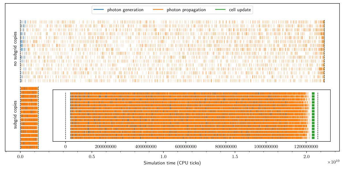
We can explore the impact of copies by looking at a visual representation of the task execution time line for both versions of the test. This can be achieved by recording the start and end time of each task during task execution, and writing out these values at the end of the run. This causes a small overhead during task execution and means we cannot reuse task data structures, so that this technique is only practical for small runs. The resulting task plot is shown in Fig. 18 for a test with 16 threads. The version without subgrid copies shows a significantly higher fraction of white gaps caused by load imbalances.
These load imbalances are caused by the relatively high cost of the propagation tasks for the central subgrid that hosts the radiation source, as is shown in Fig. 19. Since the fraction of the total computation time spent in this central subgrid is higher than the average computation capacity per thread, it is impossible to schedule the tasks in a favourable way. By making copies of the central subgrid, the total cost of this subgrid is divided among multiple subgrids, and good load balancing is restored. The improved cache efficiency that is caused by better load-balancing in turn reduces the average load per subgrid, as is also visible in the histogram.
The presence of subgrid copies is also beneficial if the central subgrid does not have a significantly higher load, but is still accessed considerably more than average, as e.g. for the Lexington test. Even in this case, we do notice a considerable impact of using subgrid copies for high thread numbers, because the copies reduce contention for the locks of the central subgrid.
4.5 Memory usage
The task-based MCRT algorithm inevitably has a larger memory footprint than a traditional MCRT algorithm because of the need to store a considerable number of photon packets during the simulation. Subgrid copies cause additional memory overhead. Apart from the grid, which still dominates memory usage for all practical applications, the photon packet buffers represent the largest contribution to the memory footprint of the algorithm, as illustrated in Fig. 20. It is therefore essential to understand what determines the required number of photon buffers and set that parameter to an appropriate value for each application.
The number of buffers in use during a simulation varies over time, as new buffers are activated by generation and propagation tasks. In the worst case scenario, every subgrid and every subgrid copy require seven active buffers: one for each neighbouring subgrid and an additional buffer to store photon packets that have been absorbed locally. In practice, not all these buffers will necessarily be activated, since some parts of the grid could receive no or very little photon packets. Moreover, each queued propagation task requires a buffer that is not linked to any subgrid. The number of queued tasks increases with the number of queues (and hence with the number of threads) and in the worst case scenario can be predicted from the maximum number of tasks in each queue. In runs with diffuse re-emission, scheduled re-emission tasks in the shared queue also contribute to the buffer requirements. In order to estimate the memory usage of the buffers, we need to measure the maximum queue load, and explore how it varies for different numbers of threads, different numbers of subgrids, and different MCRT parameters.
The maximum number of tasks among all per-thread queues and the maximum number of active buffers for our tests is shown in Fig. 21. As expected, the number of active buffers is a strong function of the number of subgrids, supplemented with an apparently linear dependence on the number of threads. The maximum number of tasks in any of the thread queues is approximately independent of the number of threads, or in other words, the queue load is approximately linear in the number of threads as well. Overall, the number of tasks that is waiting in a queue is low due to our adopted task execution strategy.
There are two notable exceptions to these observations. The Lexington test with a low number of subgrids shows a sharp increase in buffers and queued tasks for high thread numbers. This is caused by the load imbalances we noted before, which lead to the creation of an excessively high number of prematurely scheduled propagation tasks. The Strömgren test for a high number of subgrids does not show a linear dependence of the number of buffers on the number of threads, linked to the observed decrease in queue load with thread number. This indicates that tasks are executed very efficiently in this case; recall that these runs are dominated by overhead.
To obtain a practical model for predicting the memory requirements for a run, we focus on the two intermediate cases (with and cell subgrids), and fit a linear function to the number of buffers. These fits are also shown in Fig. 21. If we write the linear function as
| (3) |
then all fits have values for in the range for the Strömgren test and in the range for the Lexington test. This means that in practice only about half of the subgrid buffers are active at the same time. Except for the clearly aberrant fit, the coefficients all have values in the range , confirming that the average queue load is indeed quite low.
We conclude that the function (3) with and provides a conservative practical estimate for the number of buffers, provided that the selected subgrid size results in a small load imbalance and idle time.
| Data structure | Hydrogen-only mode | Full mode |
|---|---|---|
| (Strömgren test) | (Lexington test) | |
| photon buffer | 17.2 KB | 37.52 KB |
| single cell | 96 bytes | 310 bytes |
| cell subgrid | 6.46 KB | 20.0 KB |
| cell subgrid | 48.5 KB | 156 KB |
| cell subgrid | 384 KB | 1.22 MB |
| cell subgrid | 3.00 MB | 9.75 MB |
For convenience, the size of the individual components that dominate the memory load is shown in Table 1 for the two main MCRT modes supported by CMacIonize 2.0: the hydrogen-only mode used by the Strömgren test and the full physics mode used by the Lexington test. Note that the code needs to be configured explicitly to use the hydrogen-only mode that uses less memory, and that these sizes are likely to change when additional physics are added to the code.
5 Extensions of the algorithm
5.1 Extended sources
The algorithm as discussed so far has assumed that photon packets are emitted by discrete sources with a well-defined position. However, this need not be the case. Radiation could be incoming from an external radiation field such as the cosmic UV background, or could be emitted by a smooth source such as a stellar surface or a galactic luminosity distribution. For these extended sources, the photon packet generation task does not only provide the packet’s initial energy and propagation direction, but also draws a random starting position from the source’s spatial distribution. This position can be anywhere in the simulation box, so that an extended source cannot be associated with a particular subgrid. Therefore, a photon packet generation task for an extended source uses multiple output photon buffers, one for each subgrid in the simulation. For every newly created photon packet, the task locates the subgrid containing the starting position and adds the packet to the corresponding buffer.
After all photon packets for an extended source have been created, output buffers that are only partially filled still contain photon packets that have not been scheduled. A separate task of a new type is then created to flush these buffers. This task performs a simple iteration over all extended source output buffers and creates a photon packet propagation task for each one that is non-empty.
The photon packet generation tasks for a given extended source need exclusive access to all of the source’s output buffers. As a result, only one such task can be executed at any given time. In a simulation where a particular extended source acts as the dominant or only source of photon packets, this bottleneck can have a significant effect on the overall parallel efficiency. The problem can be overcome by providing multiple sets of the extended source photon packet output buffers, effectively treating the dominant source as multiple lower-luminosity sources.
5.2 Dust radiative transfer
The algorithm presented in Sect. 2 and implemented in CMacIonize 2.0 addresses photoionization simulations. The technique could be adjusted or extended for other MCRT applications in a straightforward fashion. In this section we consider some of the issues related to performing dust MCRT using a variation of our algorithm, without actually developing an implementation. The interactions between the radiation and the medium now include absorption, scattering and thermal re-emission (at longer wavelengths).
Radiation field
Tracking the local radiation field as a function of wavelength (Lucy 1999; Niccolini et al. 2003) is a trivial extension of our mechanism for tracking the ionisation state of the medium. Because multiple values need to be stored per cell (one per wavelength bin), the memory footprint of a subgrid increases, possibly affecting the caching efficiency and thus the optimal number of cells in a subgrid.
Forced scattering
The optical depths in dust simulations are often quite low (), causing many photon packets to escape the spatial domain without interacting with the medium. The forced scattering technique (Cashwell & Everett 1959) overcomes this problem by forcing an interaction within the simulation box. The random interaction optical depth for a photon packet is sampled from a truncated exponential distribution and the photon packet weight is adjusted to compensate. This requires knowledge of the total optical depth along the photon packet’s path, while this knowledge is only available after propagating the photon packet. To avoid performing the grid traversal twice, codes using this technique usually record details for the complete path so that this information can be used to determine both the total optical depth and the actual scattering location. Within our distributed-grid algorithm, however, recording information about each cell crossed by a photon packet is impractical because it would massively increase the memory footprint of the photon packet buffers. It would be straightforward and possibly even more efficient to perform the grid traversal twice. One can store the photon packets leaving the simulation box at the end of the preliminary propagation step in dedicated buffers and create a new task to relaunch these photon packets for the actual propagation step.
Peel-off
Other than determining the radiation field in the simulation box, one is often interested in creating synthetic observations of the simulated model, such as spectra or images, from a given line of sight. To create these observables, the peel-off technique (Yusef-Zadeh et al. 1984) is used, whereby a photon packet with an appropriate weight is sent towards the observer during each regular emission and scattering event. In an extended version of our task-based algorithm, peel-off photon packets could be handled by the propagation task that also handles the preliminary photon packets in the forced scattering technique. When a peel-off photon packet reaches the boundary of the simulation box, it is then handed off to a task that will record its contribution to the observation. Because multiple such tasks may run at the same time, the recording data structure must be accessed in a thread-safe way. This can be accomplished through some form of locking, perhaps using atomic operations, or by providing a private copy of the data structure for each execution thread.
Thermal emission
Once the radiation field in each cell has been determined during a first photon packet emission phase, the corresponding dust emission spectrum can be calculated. The spectrum can be obtained either from the energy balance equation, if assuming local thermal equilibrium, or by determining the temperature probability distribution of a set of representative dust grains (Camps et al. 2015). Because the calculation depends solely on information stored for each cell (in addition to constant dust material properties), it can be performed for each subgrid separately and thus easily in parallel. The same task can also act as a thermal emission source, generating new photon packets from the spectrum for each cell and placing them into a buffer associated with the local subgrid.
5.3 Resonant line transfer
The basic photon packet life cycle for tracing a resonant emission line such as Lyman- through an interstellar medium is very similar to the cycle described for our algorithm in Sect. 2. Usually the relevant gas densities, chemical abundances and ionization states are considered to be known in advance of the simulation. As a result, there is no need to track the local radiation field during the simulation, simplifying that part of the algorithm. Often the main interest is to calculate the overall attenuation and the precise line shape for a given line of sight. This is usually accomplished using the peel-off technique, which can be implemented as a straightforward extension of the task-based algorithm as described in Sect. 5.2.
There is, however, a complication related to the high optical depths encountered by photon packets with a wavelength near the line resonance. Such a photon packet can easily experience many thousands of scatterings in a very compact region before its wavelength shifts sufficiently far from the line centre to allow escape. If this ‘scattering region’ happens to straddle a subgrid boundary, the photon packet will be sent back and forth between subgrids countless times, significantly degrading the performance of the algorithm. This issue can be overcome by making subgrids overlap each other at their respective boundaries, perhaps by the size of a cell. As long as the state of the medium is constant during the simulation (i.e. no radiation field tracking), this is fairly trivial to implement. Otherwise, the information recorded for the overlapping cells needs to be aggregated at the end of each photon packet propagation phase.
5.4 Radiation hydrodynamics
CMacIonize 2.0 can also be used as a full radiation hydrodynamics code. In this configuration, the grid structure used for the radiation phase is also used by the finite volume solver in the hydrodynamics phase. Our task-based implementation is very similar to that in swift (Schaller et al. 2016), i.e. appropriate hydrodynamical tasks are created for each subgrid and for the interactions between neighbouring subgrids. The radiation and integration phases are separated to avoid any issues caused by the differences in scheduling strategies.
As in CMacIonize 1.0, the radiation phase can be scheduled after every time step or at regular simulation time intervals. The coupling between the two phases is affected by a single loop over all cells that updates the pressure or the energy according to the neutral fractions in the cell. Moreover, CMacIonize 2.0 also supports a more elaborate coupling scheme, whereby the heating caused by photoionization is directly used as an energy source term, and is balanced by a temperature-dependent cooling rate given by interpolation on pre-computed cooling tables. These various coupling modes can be selected at run time by adjusting the parameter file.
5.5 Spatial grids
The algorithm presented in Sect. 2 assumes a cuboidal spatial domain partitioned into subgrids according to a regular Cartesian grid, with subgrids that in turn have cells on a regular grid. Load imbalances between spatial regions can be addressed by duplicating the relevant subgrids (see Sect. 2.5). However, there are no provisions for varying the grid resolution depending on the density of the medium or on other local characteristics of the simulated model.
An obvious solution is to place the subgrids on the leaf nodes of an octree or some other hierarchical grid similar to the adaptive mesh refinement (AMR) grids used by many hydrodynamical codes. This requires adjustments to the methods for selecting the appropriate neighbour when a photon packet leaves a subgrid, and for locating the subgrid containing the starting position of a photon packet to begin with. Other than this, however, the task-based algorithm would remain largely the same.
One could also allow the individual subgrids to be subdivided into cells using a different type of grid, for example an octree or even an unstructured Voronoi mesh. However, the extra computational complexity and the larger subgrid memory footprint caused by such schemes would most likely eradicate the efficiency benefits of the presented task-based algorithm.
In the current implementation of CMacIonize 2.0, the task-based algorithm is restricted to the regular grids described in Sect. 2. However, it is still possible to run CMacIonize 2.0 using the non task-based version of the algorithm previously provided by CMacIonize 1.0, which supports both AMR and Voronoi grids.
5.6 Distributed memory
The algorithm described in Sect. 2 assumes that all parallel execution threads can access a common memory space. This implies that the algorithm runs in a shared memory environment on a single compute node and is thus limited to the memory available on a single node. For a typical state-of-the-art node this means a memory size of 200 GB or a grid resolution of approximately cells. Larger memory sizes (up to 10 TB) are available, and we have successfully tested the algorithm using a grid on a 1.5 TB node.
To support larger grids, however, the task-based algorithm would need to be ported to a distributed memory environment, where each execution thread (or small set of threads) runs in a separate process with its own private memory space. These processes can be distributed over multiple compute nodes and they cooperate by exchanging messages over a network interconnect. While this setup allows combining the resources of a potentially large number of compute nodes, it requires an explicit decomposition of the data structures and the computational work involved in the algorithm, combined with a suitable communication strategy to exchange information and synchronise the different processes.
In such an environment, subgrids (or subgrid copies) would be distributed among the available processes. Radiation sources or copies of sources can likewise be distributed. Neighbouring subgrids may now reside in a different process, so that photon packets crossing the corresponding subgrid boundary need to be sent to the corresponding process before a subsequent photon packet propagation task can be created. At least in principle, this does not require many changes to the heart of our task-based MCRT algorithm, because the infrastructure for partitioning the spatial domain and for storing and exchanging photon packets is already in place. The adjustments are essentially of a technical nature. For example, one needs a new task type responsible for sending photon packet buffers to another process, and a mechanism that regularly checks for incoming messages as part of the routine that obtains a new task for a thread.
The most important challenge, though, is to devise a strategy for distributing subgrids and radiation sources among the processes and compute nodes in such a way that the total computational load per compute node is balanced. We have experimented with a distributed memory version of the task-based algorithm and verified that it indeed works. However, implementing an appropriate load-balancing strategy is outside the scope of this work, and CMacIonize 2.0 does not include a distributed memory version of the task-based algorithm.
6 Conclusion
Modern hardware architectures have a complex memory layout that favours algorithms with predictable and localised memory access patterns. This is especially true for MCRT simulations, which require a limited amount of calculation relative to the size of the data structures being accessed, and hence are strongly memory-bound. Using a novel implementation in the photoionization code CMacIonize 2.0, we showed that the MCRT algorithm can be adjusted to produce a much more optimal memory access pattern by subdividing the grid used to discretize the physical domain into many smaller subgrids. The standard photon packet propagation phase of the MCRT algorithm can be reconstructed by executing separate propagation tasks for these subgrids and storing photon packets that transition between subgrids in temporary buffers. The resulting algorithm has the same accuracy as a traditional algorithm, but is 2 to 4 times faster. The new algorithm shows good strong scaling on shared-memory systems, and has been successfully used on systems with up to 64 shared-memory threads, and with grid sizes of up to . We showed that optimal performance is the result of a trade-off between improved cache efficiency and increased overhead, mainly determined by the size and number of subgrids. We derived a heuristic model to determine the expected memory requirements for a simulation.
The new algorithm can be extensively analysed through run time diagnostics that are available without noticeable overhead, which allows exposing bottlenecks and load imbalances. For example, subgrids that experience an above-average computational load can be duplicated to increase concurrency and restore proper load balancing. This illustrates how the new algorithm separates physical from technical aspects, and allows addressing the latter without interfering with the former.
We also discussed how our new algorithm can be adapted for other MCRT applications, e.g. dust radiative transfer and resonant line transfer. We found that many existing techniques can be ported to our task-based approach with small modifications, so that the algorithm presented here is generally applicable. More fundamentally, perhaps, we showed that optimising memory access patterns in a memory-bound algorithm can yield significant performance gains.
Acknowledgements
BV acknowledges partial support by STFC grant ST/M001296/1, and currently receives funding from the Belgian Science Policy Office (BELSPO) through the PRODEX project “SPICA-SKIRT: A far-infrared photometry and polarimetry simulation toolbox in preparation of the SPICA mission” (C4000128500). During development use was made of the DiRAC Data Intensive service at Leicester, operated by the University of Leicester IT Services, which forms part of the STFC DiRAC HPC Facility (www.dirac.ac.uk). The equipment was funded by BEIS capital funding via STFC capital grants ST/K000373/1 and ST/R002363/1 and STFC DiRAC Operations grant ST/R001014/1. DiRAC is part of the National e-Infrastructure. This work also used the DiRAC@Durham facility managed by the Institute for Computational Cosmology on behalf of the STFC DiRAC HPC Facility (www.dirac.ac.uk). The equipment was funded by BEIS capital funding via STFC capital grants ST/P002293/1, ST/R002371/1 and ST/S002502/1, Durham University and STFC operations grant ST/R000832/1. DiRAC is part of the National e-Infrastructure. Additional computational resources (Stevin Supercomputer Infrastructure) and services used in this work were provided by the VSC (Flemish Supercomputer Center), funded by Ghent University, FWO and the Flemish Government – department EWI.
References
- Agostinelli et al. (2003) Agostinelli, S., Allison, J., Amako, K., et al. 2003, Nuclear Instruments and Methods in Physics Research Section A: Accelerators, Spectrometers, Detectors and Associated Equipment, 506, 250
- Alvelius (1999) Alvelius, K. 1999, Physics of Fluids, 11, 1880
- Behrens et al. (2018) Behrens, C., Byrohl, C., Saito, S., & Niemeyer, J. C. 2018, A&A, 614, A31
- Bisbas et al. (2015) Bisbas, T. G., Haworth, T. J., Williams, R. J. R., et al. 2015, Mon. Not. R. Astron. Soc., 453, 1324
- Bordner & Norman (2012) Bordner, J. & Norman, M. L. 2012, in Proceedings of the Extreme Scaling Workshop, BW-XSEDE ’12 (USA: University of Illinois at Urbana-Champaign)
- Borrow et al. (2018) Borrow, J., Bower, R. G., Draper, P. W., Gonnet, P., & Schaller, M. 2018, arXiv, arXiv:1807.01341
- Camps & Baes (2020) Camps, P. & Baes, M. 2020, Astronomy and Computing, 31, 100381
- Camps et al. (2015) Camps, P., Misselt, K., Bianchi, S., et al. 2015, A&A, 580, A87
- Cashwell & Everett (1959) Cashwell, E. D. & Everett, C. J. 1959, A practical manual on the Monte Carlo method for random walk problems, International tracts in computer science and technology and their application (Oxford: Pergamon Press)
- Ferland (1995) Ferland, G. 1995, in The Analysis of Emission Lines: A Meeting in Honor of the 70th Birthdays of D. E. Osterbrock & M. J. Seaton, ed. R. Williams & M. Livio, 83
- Ferland et al. (2017) Ferland, G. J., Chatzikos, M., Guzmán, F., et al. 2017, Rev. Mex. Astron. Astroph., 53, 385
- Gonnet et al. (2016) Gonnet, P., Chalk, A. B. G., & Schaller, M. 2016, arXiv e-prints, arXiv:1601.05384
- Gonnet et al. (2013) Gonnet, P., Schaller, M., Theuns, T., & Chalk, A. B. G. 2013, ArXiv e-prints [arXiv:1309.3783]
- Harries et al. (2019) Harries, T. J., Haworth, T. J., Acreman, D., Ali, A., & Douglas, T. 2019, Astronomy and Computing, 27, 63
- Hubber et al. (2016) Hubber, D. A., Ercolano, B., & Dale, J. 2016, MNRAS, 456, 756
- Lucy (1999) Lucy, L. B. 1999, A&A, 344, 282
- Lund et al. (2019) Lund, K., Wood, K., Falceta-Gonçalves, D., et al. 2019, MNRAS, 485, 3761
- Niccolini et al. (2003) Niccolini, G., Woitke, P., & Lopez, B. 2003, A&A, 399, 703
- Nordlund et al. (2018) Nordlund, Å., Ramsey, J. P., Popovas, A., & Küffmeier, M. 2018, Mon. Not. R. Astron. Soc., 477, 624
- Péquignot et al. (2001) Péquignot, D., Ferland, G., Netzer, H., et al. 2001, in Astronomical Society of the Pacific Conference Series, Vol. 247, Spectroscopic Challenges of Photoionized Plasmas, ed. G. Ferland & D. W. Savin, 533
- Price (1969) Price, M. J. 1969, Astrophys. Space Sci., 4, 182
- Sartorio et al. (2019) Sartorio, N. S., Vandenbroucke, B., Falceta-Goncalves, D., Wood, K., & Keto, E. 2019, MNRAS, 486, 5171
- Schaller et al. (2016) Schaller, M., Gonnet, P., Chalk, A. B. G., & Draper, P. W. 2016, arXiv e-prints, arXiv:1606.02738
- Smith et al. (2015) Smith, A., Safranek-Shrader, C., Bromm, V., & Milosavljević, M. 2015, MNRAS, 449, 4336
- Steinacker et al. (2013) Steinacker, J., Baes, M., & Gordon, K. D. 2013, Ann. Rev. Astron. Astrophys., 51, 63
- Vandenbroucke et al. (2019) Vandenbroucke, B., Sartorio, N. S., Wood, K., et al. 2019, MNRAS, 485, 3771
- Vandenbroucke & Wood (2018) Vandenbroucke, B. & Wood, K. 2018, Astron. Comput., 23, 40
- Vandenbroucke et al. (2018) Vandenbroucke, B., Wood, K., Girichidis, P., Hill, A. S., & Peters, T. 2018, Mon. Not. R. Astron. Soc., 476, 4032
- White et al. (2016) White, C. J., Stone, J. M., & Gammie, C. r. F. 2016, ApJS, 225, 22
- Wood et al. (2004) Wood, K., Mathis, J. S., & Ercolano, B. 2004, Mon. Not. R. Astron. Soc., 348, 1337
- X-5 Monte Carlo Team (2003) X-5 Monte Carlo Team. 2003, MCNP — A General Monte Carlo N-Particle Transport Code, Version 5, revised 2/1/2008 edn., Vol. Volume I: Overview and Theory (Los Alamos National Laboratory)
- Yusef-Zadeh et al. (1984) Yusef-Zadeh, F., Morris, M., & White, R. L. 1984, ApJ, 278, 186