Option Pricing Under a Discrete-Time Markov Switching Stochastic Volatility with Co-Jump Model
Abstract
We consider option pricing using a discrete-time Markov switching stochastic volatility with co-jump model, which can model volatility clustering and varying mean-reversion speeds of volatility. For pricing European options, we develop a computationally efficient method for obtaining the probability distribution of average integrated variance (AIV), which is key to option pricing under stochastic-volatility-type models. Building upon the efficiency of the European option pricing approach, we are able to price an American-style option, by converting its pricing into the pricing of a portfolio of European options. Our work also provides constructive guidance for analyzing derivatives based on variance, e.g., the variance swap. Numerical results indicate our methods can be implemented very efficiently and accurately.
keywords
option pricing; stochastic volatility; co-jump; Markov switching; average integrated variance1 Introduction
The stochastic volatility with co-jump (SVCJ) model introduced by Eraker et al. 2003 is commonly used to model the price dynamics for an underlying financial asset, because it is able to capture leptokurtic, skewness, and volatility clustering observed in real-world data. The SVCJ model simultaneously considers stochastic volatility, jumps in return, and jumps in volatility, generalizing the jump-diffusion model in Merton 1976, the stochastic volatility model in Heston 1993, and the stochastic volatility/jump-diffusion model in Bates 1996, which are all special cases of SVCJ. Empirical evidence supporting the presence and importance of stochastic volatility with jumps in both return and volatility is documented in Eraker et al. 2003, and surveys of critical developments in the SVCJ model can be found in Eraker 2004, Broadie et al. 2007, Johannes et al. 2009, Collin-Dufresne et al. 2012, Bandi and Renò 2016, Du and Luo 2019 and references therein. SVCJ models primarily price options using Fourier transform methods.
However, Li et al. 2008 and Kou et al. 2017 point out that the SVCJ model cannot sufficiently capture volatility clustering, especially for scenarios with persistently high levels of volatility such as the period from Feb 28 to May 15, 2020, since the CIR process used in the SVCJ model assumes rapid mean reversion of volatility. Grasselli 2017 observes that the volatility process in the SVCJ model spends much time close to zero, so once an extreme value in volatility is reached, the preference for moving back to zero volatility leads to an excessively rapid mean-reversion speed. Eraker 2004 also empirically observed slower mean-reversion speed improving performance of their model in the out-of-sample period. Here we also refer to the SVCJ model with CIR process as the classical SVCJ model.
To address some of the shortcomings of the classical SVCJ model, we propose a discrete-time Markov switching stochastic volatility with co-jump (MS-SVCJ) model where the volatility is composed of a Markov switching (MS) process and a jump process. Naik 1993, Timmermann 2000, and Guo 2001 pointed out that MS processes can model the persistence of volatility. For example, Naik 1993 stressed that, “by choosing the parameters appropriately, we can model different levels of persistence of the volatility process in the high and low states.” Moreover, Timmermann 2000 stated that “Markov switching models can generate a wide range of coefficients of skewness, kurtosis and serial correlation even when based on a very small number of underlying states.” Similar arguments are made in related literature, e.g., Pan 2002, Alizadeh et al. 2002, Eraker 2004, Bakshi et al. 2006, Adrian and Rosenberg 2008, Christoffersen et al. 2009, Christoffersen et al. 2010, Chourdakis and Dotsis 2011.
In addition, since the MS process can distributionally approximate any diffusion stochastic process, we can approximate the CIR process by adjusting the parameters of the MS process. Detailed approximation implementations can be found in Lo and Skindilias 2014, Cai et al. 2015 and Cui et al. 2017. The proposed model can distributionally approximate the classic SVCJ model, so it is more robust and flexible than the classical SVCJ model. In short, the proposed model overcomes some limitations of the classical SVCJ model while retaining its advantages.
For pricing European options under the proposed model, we consider the method based on average integrated variance (AIV) developed by Hull and White 1987, in which the option price under the stochastic volatility model is expressed as the expectation of the Black-Scholes formula with variance replaced by AIV. Although this provides a formal solution for the option price, the probability distribution of AIV is generally difficult to obtain, which makes the practical application of this method challenging. For our MS-SVCJ model, we face the same challenge.
We consider a discrete-time MS volatility process with finite state space, so there are a finite number of sample paths of volatility, which means the value space of AIV is also finite. Thus, theoretically we can find the probability distribution of AIV by enumerating all the sample paths of volatility, but such enumeration is generally not computationally feasible, so we propose the recursive recombination (RR) algorithm to efficiently compute the probability distribution of AIV. Then we derive a pricing formula that leads to an analytical solution for European options under our proposed model. Numerical experiments demonstrate the effectiveness of the RR algorithm.
Our work extends the existing literature on European option pricing in several ways. First, without the jumps in volatility, the proposed model becomes the MS-SVJ model, so our analytical solution for European options applies to the MS-SVJ model with general jump size distribution. Second, removing jumps from both the volatility and asset price, the proposed model reduces to the MS-SV model, so using our analytical solution for the MS-SV model avoids having to solve a set of intractable ordinary differential equations when pricing options, as in Naik 1993, Guo 2001, and Fuh et al. 2012, or using numerical inverse Fourier transform methods, as in Buffington and Elliott 2002, Elliott et al. 2006, and Liu et al. 2006.
We also consider the pricing of American-style derivatives (see Broadie and Detemple 1996), applying the approach proposed by Laprise et al. 2006 by leveraging our analytical solutions for pricing European options. In the approach, the pricing of an American-style option can be converted into the pricing of a basket of European options. We compare our results with the least squares Monte Carlo simulation approach by Longstaff and Schwartz 2001. For more discussion of the application of Monte Carlo simulation approaches to American-style derivatives, refer to Broadie and Glasserman 1997a, Broadie and Glasserman 1997b or Fu et al. 2001. Our numerical examples further illustrate the effectiveness of our approach.
In sum, our work contributes to the option pricing research literature as follows:
- •
We provide an analytical pricing formula for European options under a discrete-time MS-SVCJ model that is more robust and flexible than the classical SVCJ model and can explain volatility clustering for high levels of volatility.
- •
We develop an efficient algorithm to obtain the probability distribution for AIV, which can also be applied to other related volatility derivatives, e.g., the variance swap.
- •
Our analytical solution for European option prices applies to several well-known models in the literature, including the MS-SVJ model with general jump size distribution. For the MS-SV model, our approach also has computational advantages over existing option pricing methods, by eliminating having to numerically solve a set of ordinary differential equations.
- •
We price American-style options by leveraging the efficiency of our analytical pricing solution for European options.
The remainder of the paper is organized as follows. In Section 2, we construct the MS-SVCJ model and analyze the AIV probability measure. Section 3 develops the option valuation under the MS-SVCJ model. In Section 4, we present the RR algorithm and analyze its computational complexity. Numerical results for pricing both European options and American-style options are presented in Section 5. Section 6 concludes and discusses future research.
2 Theoretical Framework
In this section, we build the Markov switching stochastic volatility with co-jump (MS-SVCJ) model for the underlying asset and define the AIV probability measure.
2.1 Model Setting
Under the MS-SVCJ model, the underlying asset price is assumed to follow a jump-diffusion process, and the asset volatility is also stochastic. Specifically, the dynamics are specified by the following two equations under the risk-neutral probability measure :
| (1) | ||||
where is standard Brownian motion; is a Poisson jump process with intensity ; the proportional jumps are independent and identically distributed (i.i.d.) with ; follows a discrete-time Markov switching (MS) process; which states the impact of jumps in asset price on variance is the proportional and exponentially attenuating (PEA) process; , , and are mutually independent. We regard the risk-free interest rate as constant.
The main distinctive feature of the proposed model is that the variance process is composed of two components: the first explains the exogenous dynamics of variance, e.g., due to changes in the economy and company announcements, and the second explains the endogenous movement in variance due to jumps in the asset, similar to Duffie et al. 2000. The proposed model assumes the first part follows an MS process and the second part follows the jump process related to jump in asset price. In what follows, we provide detailed specifications of the two processes.
We assume follows a discrete-time Markov switching (MS) process with finite state space and constant time step , and one-step transition probability matrix , i.e., The MS process has been shown to model reasonably well most of the stylized facts of volatility, volatility clustering and mean-reversion. See Naik 1993, Rydén et al. 1998, Duan et al. 2002, Aingworth et al. 2006, Rossi and Gallo 2006. Furthermore, compared with affine models for volatility, e.g. the square-root model, the MS process can better capture the clustering in different volatility levels and the varying mean-reversion speeds of volatility.
The second part takes into account the sudden movement in variance caused by jumps in the asset price. Here, we model as the product of two components, one representing the instantaneous shock size of variance due to the jump in asset return, and the other representing the dynamics of this shock over time. This dependence structure of jumps in asset price and volatility was proposed theoretically by Barndorff-Nielsen and Shephard 2001, Klüppelberg et al. 2004. Todorov 2011 empirically identified the effectiveness of this structure. Specifically, we give the following description of .
Definition 2.1
The is a proportional and exponentially attenuating (PEA) process if for the jump in asset price at , where
In the above representation, the term is the shock size of variance caused by the jump in asset price, and the shock size is proportional to the square of log-jump in asset price with proportional coefficient , which is consistent with the definition of variance expressed as the average of the quadratic function of the decentralized logarithm of the return. As a memory function, the term indicates that the shock of the jump tails off exponentially with attenuating factor and duration , which is analogous to the CARMA kernel in Brockwell 2001. Following J.P.Morgan/Reuters 1996, we assume that the duration is finite and fixed.
2.2 Probability Measure
Hull and White 1987 show that the option price under the stochastic volatility model can be computed as the expectation of the Black-Scholes formula with variance replaced by average integrated variance (AIV). We derive a similar result in Section 3.1 when the diffusive innovation to the asset price process is independent of volatility. Under the proposed model, AIV during the interval can be expressed as
| (2) |
Thus, AIV can be expressed as a sum of two terms, one due to the MS process and the other due to the PEA process. Since AIV due to the MS process plays a key role, we first provide the following description. We assume that is chosen such that is integer-valued, so that is the total number of time steps. Since the information up to current time is available, we also assume the initial state of is known. The MS process generates sample path during . Since is a piecewise constant process, we can represent the sample path as the following tuple form: where is fixed.
For notational simplicity, we write as . In the following, the MS process will be rewritten as to highlight its discretization, and henceforth, the above sample path will be expressed as with weight and probability given by
Here, we denote the set of all sample paths as , the sample path space for .
Figure 1 illustrates an example of sample path .
AIV due to the MS process, which is the first term defined in Equation , is given by
which is a random variable with probability distribution derived from and with value space and corresponding probability Clearly, , and in general, the number of possible values of is far less than the total number of sample paths of , and we have the following proposition (see Appendix A for proof).
Proposition 2.2
.
3 Option Valuation
3.1 European Option Pricing
In this section, we price a European call option under the proposed model described by Equation . A European put option can also be priced by the same method. First, we provide the following formal solution for the European call option price (see Appendix B for proof).
Lemma 3.1
Under the MS-SVCJ model, the price of a European call option with strike price , maturity , and initial price can be written as
| (3) |
where is the number of jumps in the asset price up to ; is an -dimensional random vector of jump sizes; is the sample path space of ; is the asset price at the maturity given and .
Before deriving a tractable solution, we need the probability distribution of . Using the lemma in Hull and White 1987, we can derive the following (see Appendix C details):
| (4) |
where is the cumulative effect of jumps in the asset price with , , and is the realization of given and ,
We now focus our attention on the quantity . For simplicity and technical convenience, we assume that all jumps during the interval occur at the beginning of the interval at time ; the impact of this jump time assumption on the option price is negligible, as discussed in Appendix I and illustrated numerically in Section 5.1. Hence,
| (5) | ||||
From Lemma 3.1, combined with Equations and , we have:
| (6) | ||||
where is the classical Black-Scholes formula as a function of initial stock price , volatility , risk-free rate , maturity , and strike price . Substituting Equation into Equation yields the price of a European call option (see Appendix D for proof).
Theorem 3.2
Under the MS-SVCJ model, the price of a European call option with strike price , maturity , and initial underlying asset price is given by
where , .
in Theorem 3.2 is a bivariate random variable, so the -dimensional integral in Lemma 3.1 has been replaced by a double integral in Theorem 3.2. In many special cases, e.g., when the jump distribution is lognormal, the probability distribution of can be expressed explicitly, so that can be easily computed (see Appendix E for proof).
Proposition 3.3
For , , the probability density function of is given by
For lognormally distributed jump sizes, Proposition 3.3 provides an analytical expression for the option price, different from the traditional solution using numerical Fourier transform inversion.
Moreover, under a general jump size distribution, the following corollary gives the option price for the MS-SVJ model, a special case of MS-SVCJ model (see Appendix F for proof).
Corollary 3.4
Under the Markov switching stochastic volatility jump-diffusion (MS-SVJ) model, which can be recovered by setting in the MS-SVCJ model, and the jump size follows a general distribution, the price of a European call option is given by where is the European call option price under the jump-diffusion model.
Thus, given the probability distribution , the option price only depends on . When follows a normal distribution, a mixed-exponential distribution, or a general discrete distribution, can be obtained via various approaches, such as Merton 1976, Kou 2002, Kou and Wang 2004, Cai and Kou 2011, or Fu et al. 2017. Hence, under the MS-SVJ model with the above jump size distribution, we also provide an analytical solution for the option price.
Moreover, we can provide an analytical option price under the MS-SV model, which overcomes the drawbacks of Naik 1993, Duan et al. 2002, Aingworth et al. 2006.
Corollary 3.5
Under the Markov switching stochastic volatility (MS-SV) model, which can be recovered by setting and the Poisson intensity in the MS-SVCJ model, the price of a European call option is given by
Proof. When and the Poisson intensity , we have , , , and .
This result is similar to Hull and White 1987, who provided a formal solution but did not specify the distribution of AIV needed for computing the option price.
3.2 American-Style Option Pricing
By leveraging our analytical solution for European option, we can provide an efficient approximation to the price of an American-style option using the approach proposed by Laprise et al. 2006. By converting the price of an American-style option to the price of a portfolio of European options, Laprise et al. 2006 designed algorithms to provide an upper bound and a lower bound for the price of an American-style option, where early-exercise opportunities were restricted to discrete points .
In order to apply the algorithms, for every interval , one only needs to compute two critical variables: and , where is the European call option value with initial asset price , strike price and maturity . For the asset price following geometric Brownian motion and the Merton jump-diffusion model, Laprise et al. 2006 provided a tractable expression for .
When the volatility follows the MS process, at any given time , volatility is a random variable with value space and corresponding probability . Hence we have,
| (7) | ||||
where is the European call option with initial asset price , strike price , maturity and initial status for the MS process in .
Theorem 3.2, Corollary 3.4, and Corollary 3.5 provide detailed solution for in for MS-SVCJ, MS-SVJ, and MS-SV models, respectively. As an example, the detailed expressions under the MS-SVCJ model can be written as follows by substituting Theorem 3.2 into (7):
| (8) | ||||
where highlights that AIV is dependent on the initial status for the MS process, and .
For the MS-SV model, we have
| (9) | ||||
Up to now, we have provided an analytical solution for option price under the proposed model with the lognormal jump size distribution. Practical application requires calculating the probability distribution of efficiently, which is addressed in the next section.
4 An Efficient Algorithm for MS-process AIV
After observing that complete enumeration (CE) based on the definition of is intractable due to the enormous computation time and consumed memory, we develop an efficient algorithm for the probability distribution called the recursive recombination (RR) algorithm.
4.1 Complete Enumeration (CE)
Based on the definition of in Section 2.2, a complete enumeration (CE) algorithm for and would traverse all sample paths and generate ; then collect distinct values to get and sum probabilities with to get . However, for the MS process with states, the complexity of CE is clearly , exponential in the number of time steps. Hence, to efficiently derive and , we propose the RR algorithm.
4.2 Recursive Recombination (RR) Algorithm
Recall from Section 2.2, for the MS process , the initial state is fixed. Here, we define a subsample path of up to step , as the first elements of a sample path , with weight and corresponding probability :
In addition, we also denote the set of all subsample paths as , which is the subsample path space for up to step .
For a subsample path , we extract three fundamental features: the weight , the length and the last element , which generate a triple . Thus, is a random variable with value space and corresponding probability .
Now we can relate to the random variable :
| (10) | ||||
We provide an example with state set , number of time steps , and initial state . In Figure 2, all the subsample paths with the same constitute . Taking as an example, eight subsample paths generate . Based on in Figure 2, Figure 3 presents the corresponding value space . As an example with , the different subsample paths and are distinct elements in , but since they have the same weight , the same length and last element, then they correspond to the same element in . Finally, based on Equation , we have , which is consistent with the definition of .
Now we present a recursive algorithm to obtain and . Since the initial state is fixed, for , we have and .
The main recursive step is based on the following proposition, where can be generated from by taking a step forward.
Proposition 4.1
The value space and the probability of follow the recursive relationship:
Continuing with the example above, Figure 4 illustrates recursion and recombination from from to . We start from , then take a step forward to generate an intermediary set without recombination. For example, and taking a step forward generate and , respectively. After recombining the same element in the intermediary set, for example and , we obtain .
Table 1 provides the RR algorithm for the value space and the probability distribution . In terms of computational complexity, we have the following result (see Appendix G for proof):
Proposition 4.2
The total number of distinct triples from step to step is bounded by ; hence the complexity of the RR algorithm is .
Since in settings of practical interest, the RR algorithm should be far superior to CE in terms of computation, which is confirmed in the next section.
Input:
| |||
Initialization:
| |||
Recursion:
| |||
Output:
|
5 Numerical Experiments
In this section, we first price the European call option under the proposed model. We conduct Monte Carlo simulation to assess the impact of the jump time assumption on the option price. After that, we discuss the result for the Bermudan call option pricing to show the effectiveness of our approach. Then we compare the proposed RR algorithm with CE, and the results highlight the computational superiority of the RR algorithm. Lastly, we provide an application example of fitting to real-market data. All numerical results are obtained using MATLAB (see Appendix H for MATLAB code) on a 2.40 GHz Intel Xeon E5-2680, 128 GB RAM computer.
5.1 European Option
Before applying our pricing method under the proposed model, we conduct a Monte Carlo simulation to assess the impact of the assumption on jump time on the option price. The parameters for the proposed model are presented in Table 2. Specifically, we follow Todorov 2011 to assign the values of duration , attenuating factor , proportional coefficient (see Appendix J).
| Parameter | Value | Parameter | Value | Parameter | Value | ||
| Maturity | Jump variance | Initial state | |||||
| Strike price | Max # jumps | State space | |||||
| Risk-free rate | Time step | Transition probability matrix | |||||
| Asset price | Duration | ||||||
| Jump intensity | Attenuating factor | ||||||
| Jump mean | Proportional coefficient |
-
max # jumps truncated at such that ; for with and values, .
Using an Euler approximation with equal subintervals, Monte Carlo simulation generates the asset price at maturity. For the case in Table 2, the option prices using Theorem 3.2, denoted by MS-SVCJ, and Monte Carlo simulation, denoted by MC, are summarized in Table 3. For the MC column, option price, standard error, and computation time are based on 10 sets of paths. MC simulation is very time-consuming, with an example of taking around hours.
| MS-SVCJ | MC Simulation | |||||
| =600 | 750 | 900 | 1200 | 1500 | ||
| Option Price | 0.9696 | 0.9680 | 0.9683 | 0.9684 | 0.9687 | 0.9689 |
| (Std Err) | (.0063) | (.0044) | (.0050) | (.0066) | (.0054) | |
| Computation Time (seconds) | 30 | 16575 | 20213 | 25014 | 28411 | 41034 |
As mentioned in Section 3.1 and Appendix I, the assumption on jump time will increase the volatility slightly, hence increase the option price slightly. On the other hand, the MC values monotonically increase with , so the option price without the assumption lies in the interval , bounding the relative error at less than and indicating that the impact of the assumption on the option price is negligible. Moreover, the option price with the assumption stays within the confidence interval of all the MC values, providing further support for the reasonableness of the assumption.
5.2 American-Style Option
For an American-style option, we apply the secant and tangent algorithms of Laprise et al. 2006 to establish bounds for its price. Under the MS-SV model, the value is a weighted sum of over the possible AIVs. We use interpolation points for the asset price, where the approximation accuracy can be improved by increasing the number of interpolation points. As a comparison, we also implement the least squares Monte Carlo simulation approach of Longstaff and Schwartz 2001 for American option pricing, denoted by LSM, based on 10 sets of independent runs with 100,000 paths for each run.
We illustrate our approach with the following example from Laprise et al. 2006: a three-year Bermudan call option with strike price , exercisable every years. For the dynamics under the MS-SV model, we set risk-free rate , dividend rate , initial state , state space , time step with the transition matrix shown in Table 2. We calculate and using Equation .
The results in Table 4 show that the upper and lower bounds derived from the secant and tangent algorithms, respectively, converge quickly with the number of interpolating points. For example, with 100 interpolating points, the upper and lower bounds are within a penny of the true price. For , option prices with different initial asset prices via the secant and tangent algorithms all stay with the confidence interval of the corresponding LSM values. In addition, the computation time for LSM is orders of magnitude higher than the time for the secant and tangent approximation approaches.
| Option Price | Computation Time | ||||||
| Algorithm | =60 | 90 | 100 | 110 | 140 | (seconds) | |
| Tangent | 50 | 1.294 | 9.846 | 14.867 | 20.848 | 43.204 | 0.41 |
| 100 | 1.302 | 9.861 | 14.883 | 20.861 | 43.212 | 0.98 | |
| 200 | 1.305 | 9.864 | 14.886 | 20.864 | 43.213 | 2.97 | |
| Secant | 200 | 1.307 | 9.868 | 14.890 | 20.867 | 43.215 | 1.64 |
| 100 | 1.311 | 9.875 | 14.897 | 20.873 | 43.219 | 0.55 | |
| 50 | 1.328 | 9.904 | 14.925 | 20.899 | 43.234 | 0.23 | |
| LSM | 1.306 | 9.866 | 14.888 | 20.860 | 43.210 | 415 | |
| (Std Err) | (.016) | (.019) | (.043) | (.020) | (.074) | ||
Next we apply our approach to price the same call option under the MS-SVCJ model, which is very similar to MS-SV model with additional jumps and co-jumps. The model parameters are the same as in Table 2, and and are calculated via Equation . The results for , and are illustrated in Table 5.
| Option Price | Computation Time | ||||||
| Algorithm | =60 | 90 | 100 | 110 | 140 | (seconds) | |
| Tangent | 20 | 1.970 | 11.624 | 16.815 | 22.845 | 44.864 | 68 |
| 50 | 2.040 | 11.723 | 16.911 | 22.932 | 44.924 | 390 | |
| 100 | 2.050 | 11.737 | 16.924 | 22.945 | 44.933 | 1504 | |
| Secant | 100 | 2.060 | 11.752 | 16.938 | 22.957 | 44.941 | 895 |
| 50 | 2.080 | 11.780 | 16.965 | 22.982 | 44.958 | 230 | |
| 20 | 2.223 | 11.977 | 17.154 | 23.157 | 45.078 | 39 | |
| LSM | 2.066 | 11.773 | 16.957 | 22.972 | 44.903 | 23934 | |
| (Std Err) | (.028) | (.082) | (.082) | (.079) | (.095) | ||
5.3 CE versus RR
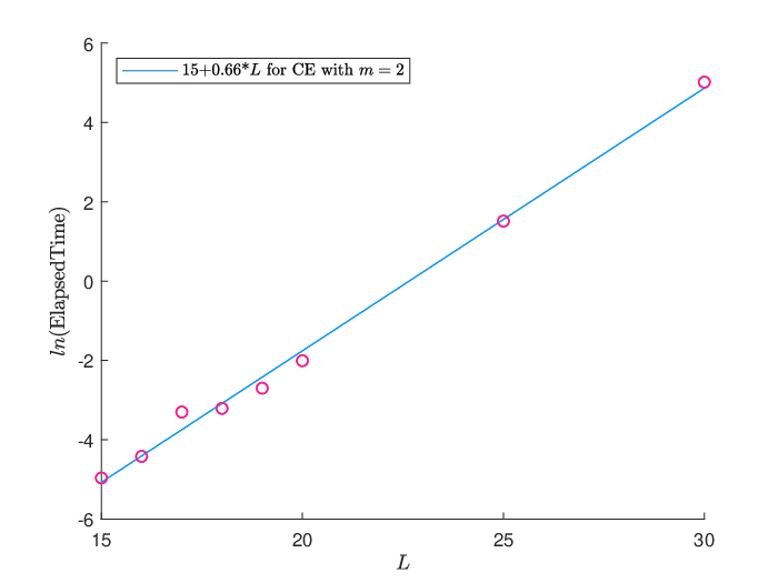
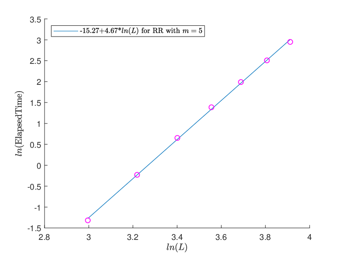
We compare the computation time for CE and the RR algorithm as a function of and , with the results provided in Tables 6 and 7, respectively. The results in Table 6 illustrate that for CE, the computation time increases exponentially with respect to the number of time steps , and the consumed memory is quickly exhausted, which limits the application of CE in practice. Comparing Table 6 with Table 7, the improvement using the RR algorithm is significant. For example, for , or , , the RR algorithm finishes within about 10 seconds.
| 15 | 16 | 17 | 18 | 19 | 20 | 25 | 30 | |
| 2 | 0.007 | 0.01 | 0.04 | 0.04 | 0.07 | 0.13 | 4.5 | 151 |
| 3 | 1.3 | 4.1 | 12 | 38 | 119 | 365 | * | * |
| 4 | 92 | * | * | * | * | * | * | * |
| 5 | * | * | * | * | * | * | * | * |
| 6 | * | * | * | * | * | * | * | * |
| 20 | 25 | 30 | 35 | 40 | 45 | 50 | |
| 2 | 0.005 | 0.006 | 0.007 | 0.008 | 0.011 | 0.013 | 0.014 |
| 3 | 0.009 | 0.013 | 0.019 | 0.024 | 0.033 | 0.040 | 0.050 |
| 4 | 0.05 | 0.11 | 0.21 | 0.39 | 0.66 | 1.05 | 1.58 |
| 5 | 0.27 | 0.8 | 1.9 | 4.0 | 7.3 | 12 | 19 |
| 6 | 1.2 | 4.2 | 10 | 22 | 38 | 60 | 87 |
To illustrate the computational complexity of both algorithms, we graph the computation time as a function of the number of time steps for both algorithms. Figure 5 shows representative plots of the performance of CE with two states and the RR algorithm with five states; additional results are provided in Appendix K. The results support the theoretical computational complexity of for CE and for the RR algorithm.
5.4 Application Example
We calibrate our model to market option prices after estimating the MS and PEA model parameters for the underlying asset prices using real data from Yahoo Finance consisting of the daily closing stock prices of IBM from January 1, 2005 to June 30, 2019. We estimate the jump process using the box-plot method. Specifically, we assume values of the daily log-return outside the range constitute jumps, where is the sampling interval length for the daily price, is the lower quartile, is the upper quartile, the interquartile range is defined as , and is a constant. After assigning , we can estimate jump intensity, mean of jump size, and variance of jump size for the jump process.
We then estimate the MS process using maximum likelihood estimation (MLE) and the PEA process using the generalized method of moments (GMM). Following the box-plot method, we decompose the full sample into two subsamples, the diffusion subsample within the range and the jump subsample outside the range . Based on the diffusion subsample, we estimate the MS process by the method provided in Perlin 2015; see Appendix L for the details. Based on the jump subsample, we estimate the PEA process by GMM provided in Todorov 2011; see Appendix M for the details. The parameters for the PEA are duration ; attenuating factor ; proportional coefficient . For the MS process, the state space is , i.e, four states with corresponding transition probability matrix
Next we discuss the model calibration procedure. The proposed model consists of three parts: the PEA process captures the correlation for model drivers, while the MS process and jump process capture the volatility of underlying asset. For illustrative purposes, in this example we fix the parameters for the PEA and MS processes estimated from historical data, and solve for the optimal parameters for the jump process by calibrating to the option market prices.
Specifically, we calibrate our model to IBM call options on July 1, 2019 with maturity months. The risk-free rate is determined by US Dollar LIBOR rates using two maturities, 1 month and 2 months, by linear interpolation to match option maturity. Similar to Cai and Kou (2011), we minimize the objective function over the set of varying parameters of the jump process, where and represent the calibrated price and the market price for the th option, respectively. To solve the optimization problem, a random search algorithm gave the final optimal solution: , , . Table 8 presents a comparison of model and market prices, where the last column shows relative biases for option price, and Figure 6 indicates that the calibration to option prices is quite good.
| Market | Model | ||||
| Strike | Bid | Ask | Mid-Price | Price | Bias |
| 125 | 15.05 | 16.85 | 15.95 | 15.83 | |
| 130 | 11.60 | 11.80 | 11.70 | 11.44 | |
| 135 | 7.60 | 7.70 | 7.65 | 7.52 | |
| 140 | 4.30 | 4.45 | 4.375 | 4.32 | |
| 145 | 2.07 | 2.16 | 2.115 | 2.10 | |
| 150 | 0.80 | 0.84 | 0.82 | 0.84 | |
| 155 | 0.28 | 0.29 | 0.285 | 0.29 | |
| 160 | 0.08 | 0.10 | 0.09 | 0.09 | |

6 Conclusions
In the paper, we propose the MS-SVCJ model to better capture volatility clustering. Under the proposed model, we derive an analytical solution for the price of European options. Due to the general nature of the model, we can apply the analytical solution to some special cases, such as the MS-SVJ model with general jump size distribution or the MS-SV model. An analytical solution for the MS-SV model avoids solving ordinary differential equations using numerical inverse Fourier transform methods. We also consider an approximation approach to price American-style options by leveraging our analytical solution for European options. To efficiently compute option prices, we propose the RR algorithm to derive the probability distribution of AIV, analyze its computational complexity, and verify its effectiveness numerically.
The empirical case study discussed in Section 5.4 uses asset prices to estimate the MS and PEA model parameters, while calibrating the jump process parameters by market option prices. In practice, market data on actual option prices can be used to calibrate all of the model parameters of any option pricing model. Although not the focus of this work, a complete calibration procedure based on only market option prices would make our algorithm more relevant to practitioners. We briefly suggest one possible approach, which adopts a two-stage calibration procedure, cf. Galluccio and Lecam 2008, Clark 2011, Tan 2012, Homescu 2014; however, determining a good procedure is definitely a critical need for further research.
The two-stage calibration procedure calibrates the MS process and jump process (the compound Poisson process and the PEA process) separately. Specifically, at the first stage, we calibrate the MS-SV model to market option prices. The approach in Britten-Jones and Neuberger 2000 appears to be well suited to our MS-SV model, since it models volatility following a MS process. In this approach, they first determine a base model reflecting one’s prior information on market, then adjust the base model to fit option prices.
At the second stage, we can calibrate CJ component of the MS-SVCJ model with the calibrated MS-SV process at the first stage. The calibration is to determine the compound Poisson process and the PEA process by minimizing the sum of an in-sample quadratic pricing error and a convex penalization term. In practice, the key is to select the convex penalization, which consists of two terms, one due to the compound Poisson process and the other due to the PEA process. Cont and Tankov 2004 used relative entropy (or Kullback-Leibler divergence) from a prior distribution as a convex penalization term. For the PEA process, since parameters for the PEA process form a Hilbert space, a quadratic function (or Tikhonov regularization) is appropriate and applied.
The methodology developed here should also be applicable in other contexts beyond option pricing, e.g., variance swap pricing, which depends highly on the AIV. Other open problems for future research include hedging under the proposed model, as well as extensions to more general models, e.g., models with general jump size distribution.
Appendix A Proof of Proposition 2.2
We denote as the number of states of sample paths of the MS process from step to step , . Thus, for each sample path of the MS process, we can get a tuple . According to the definition of the weight of a sample path of the MS process, since , , take value in state set , after merging the same states in sample path, the weight can be rewritten as where is the initial state of the MS process and is pre-determined. This leads to a surjection from tuple to weight rather than an injection due to the possibility of the different tuples generating the same weights. Thus, the number of distinct values for is less than the number of distinct tuples, which satisfies the equation for which the solution is a combinatorial problem given by , which is the number of ways to select distinct values from . Hence, we have .
Appendix B Proof of Lemma 3.1
According to the arbitrage-free pricing theory, the European option price is the expectation of the terminal payoff under the risk-neutral probability measure. At maturity , the payoff of a European call option is , so the European call option price is given by
where is the number of jumps in the asset price up to ; is an -dimensional random vector of jump sizes; is the sample path space of ; is the asset price at the maturity given and .
Appendix C Details of Derivation for
Here, we consider the conditional probability distribution of the asset price at , given jumps and the sample path of . Correspondingly, the asset price is the solution to the following stochastic differential equation:
where the volatility process is a deterministic function of time .
In terms of the analysis in Hull and White 1987, the solution to above equation is given by
where . Hence, we have
Appendix D Proof of Theorem 3.2
Appendix E Proof of Proposition 3.3
For notational convenience, we denote:
| (11) | ||||
where is the number of jumps during and the jump size distribution . When , the proof is obvious and omitted.
Next, we suppose . Before determining the joint probability density , we determine the support set of the bivariate random variable , . By the Cauchy-Schwarz inequality, we have:
| (12) |
so substituting the definition of in Equation into Equation , we have . Thus, the support set , on which we derive the joint probability density . We have:
According to Theorem 5.3.1 in Casella and Berger 2002, and are mutually independent with probability distributions and , respectively. By conditional probability, we decompose , where
which leads to the desired result.
Appendix F Proof of Corollary 3.4
When , we have and .
Since does not require the probability distribution of jump size , the expression holds for the jump size following a general distribution, so the European call option price is
where is the European call option price under the jump-diffusion model.
Appendix G Complexity of RR Algorithm
To prove the complexity of RR algorithm, we first provide the following lemma.
Lemma G.1
The number of distinct triples at step is less than .
Proof G.2
Proof. At step , the number of distinct triples can be decomposed into the product of the number of distinct values of and the number of distinct values of , which is a combinatorial problem. Obviously, the number of distinct values of is . To determine the number of distinct values of , we denote as the number of states of subsample paths of the MS process from step to step , . Thus, for each subsample path of the MS process, we can get a tuple . Similar to Proposition 2.2, we have:
where is the initial state of the MS process and is pre-determined.
According to Proposition 2.2, the number of distinct values of is less than . Hence, the number of distinct triples at step is less than .
Proposition G.3
The total number of distinct triples from step to step is less than , hence the complexity of the RR algorithm is .
Proof G.4
Proof. The total number of distinct triples from step to step is a summation of the number of distinct triples at every step . According to Lemma G.1 providing an upper bound for the number of distinct triples at step , carrying out a summation for steps, we will provide an upper bound for the total number of distinct triples from step to step ,
Hence, the total number of distinct triples from step to step is less than .
In addition, since in settings of practical interest, we have:
Appendix H MATLAB Code for RR Algorithm
Appendix I Impact of Assumption on Jump Time
We discuss the impact of the assumption that all jumps in the small interval occur at the beginning of the interval on the asset price and AIV. Since the cumulative impact on asset price does not relate to the actual times of the jumps, the asset price at does not change under the assumption. In what follows, considering the probability of a jump, we analyze the expectation bias () caused by the assumption on AIV.
First, we denote the jump probability and the expectation bias as and , respectively, when there are jumps up to maturity , given by
Second, since the sample path of the MS process and the jump during the interval do not cause the bias, we only investigate the bias caused by a jump during the interval . Given jumps up to maturity , we denote the conditional jump probability and the expectation bias as and , respectively, for jumps during the interval , given by
where
Third, we derive the detailed expression for . For the th jump at time , without or with the assumption, the cumulative effects until expiration date are, respectively:
Hence,
where and , where is a uniform distribution, since for the Poisson process with intensity , conditioned on , the joint probability distribution of the ordered arrival times of jumps is the same as the joint probability distribution of the order statistics with , .
Since , we have
Taking , , , , , , in Table 2 as an example, . The option price implies volatility , so the assumption increases volatility by , which is less than 0.002.
Appendix J Estimating Parameters in the PEA Process
We describe estimation of the parameters of the PEA process: proportional coefficient , attenuating factor and duration . For this purpose, we adopt the approach of Todorov 2011, in which the modeling of co-jumps is similar to ours, viz., the jump in variance is also proportional to the squared jump in return and exponentially decays over time.
Once a jump in return occurs, the proportional coefficient determines the corresponding increment of variance. In terms of the expressions of and in Todorov 2011, we derive the proportional coefficient .
The function in Todorov 2011 describes the evolving pattern of jump in variance, which corresponds to our function . For , through sampling points from in Todorov 2011 and implementing the least squares method, we estimated the attenuating factor with the goodness of fit, .
We select the duration , which means once there is jump in variance, our model can cover of this increment over the next 5 days. We assume a year includes 252 trading days, hence days.
Appendix K Additional Empirical Results on Computational Complexity for CE and RR
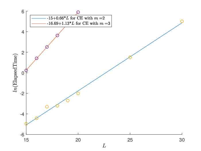
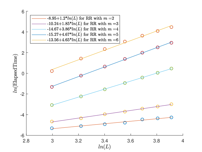
We confirm the theoretical computational complexity of the CE and RR algorithms with a larger number of states . Specifically, the computation time as a function of the number of time steps is shown in Figure 7, in line with the theoretical results and numerical experiments in the main body of the main manuscript.
Appendix L Estimation of the MS Process for the Application Example in Section 5.4
Following the standard risk premia assumptions in the literature, the asset price without jumps under the objective probability measure follows geometric Brownian motion with drift and MS stochastic volatility . To estimate the MS process, we consider the discrete version of the asset price described by
where follows a standard normal distribution. Using this result with existing MATLAB codes provided in Perlin 2015 to the diffusion subsample generating , the estimated parameters for MS process are easily obtained.
Appendix M Estimation of the PEA Process for the Application Example in Section 5.4
Given the path of the MS process , we derive closed-form expressions for variance, skewness, kurtosis of asset log-return:
| (13) | ||||
where , and , are the th moments of the log-jump distribution.
Specifically, given the path of the MS process , our original model in Equation has similar probability characteristics as the model in Todorov 2011, and Equation can be justified by Theorem 1 of Todorov 2011. Applying the generalized method of moments (GMM) estimation to the jump subsample, the estimated parameters for the PEA process are easily obtained.
Acknowledgments.
Fu gratefully acknowledges financial support from the U.S. National Science Foundation [Grant CMMI-1434419]. Li gratefully acknowledges financial support from the Natural Science Foundation of China [Grant 71671094], and the Fundamental Research Funds for the Central Universities [Grants 63185019 and 63172308]. The views and opinions expressed in this article are solely the authors own and do not reflect the business and positions of R. Wu’s affiliation.References
- Adrian and Rosenberg (2008) Adrian T, Rosenberg J (2008) Stock returns and volatility: Pricing the short-run and long-run components of market risk. J. Finance 63(6):2997–3030.
- Aingworth et al. (2006) Aingworth DD, Das SR, Motwani R (2006) A simple approach for pricing equity options with Markov switching state variables. Quant. Finance 6(2):95–105.
- Alizadeh et al. (2002) Alizadeh S, Brandt MW, Diebold FX (2002) Range-based estimation of stochastic volatility models. J. Finance 57(3):1047–1091.
- Bakshi et al. (2006) Bakshi G, Ju N, Ou-Yang H (2006) Estimation of continuous-time models with an application to equity volatility dynamics. J. Financial Econom. 82(1):227–249.
- Bandi and Renò (2016) Bandi FM, Renò R (2016) Price and volatility co-jumps. J. Financial Econom. 119(1):107–146.
- Barndorff-Nielsen and Shephard (2001) Barndorff-Nielsen OE, Shephard N (2001) Non-Gaussian Ornstein-Uhlenbeck-based models and some of their uses in financial economics. J. R. Statist. Soc. B 63(2):167–241.
- Bates (1996) Bates DS (1996) Jumps and stochastic volatility: Exchange rate processes implicit in Deutsche Mark options. Rev. Financial Stud. 9(1):69–107.
- Britten-Jones and Neuberger (2000) Britten-Jones M, Neuberger A (2000) Option prices, implied price processes, and stochastic volatility. J. Finance 55(2):839–866.
- Broadie et al. (2007) Broadie M, Chernov M, Johannes M (2007) Model specification and risk premia: Evidence from futures options. J. Finance 62(3):1453–1490.
- Broadie and Detemple (1996) Broadie M, Detemple J (1996) American option valuation: New bounds, approximations, and a comparison of existing methods. Rev. Financial Stud. 9(4):1211–1250.
- Broadie and Glasserman (1997a) Broadie M, Glasserman P (1997a) Monte Carlo methods for pricing high-dimensional American options: An overview. Net Exposure 3:15–37.
- Broadie and Glasserman (1997b) Broadie M, Glasserman P (1997b) Pricing American-style securities using simulation. J. Econom. Dynam. Control 21(8/9):1323–1352.
- Brockwell (2001) Brockwell PJ (2001) Lévy-Driven CARMA processes. Ann. I. Stat. Math 53(1):113–124.
- Buffington and Elliott (2002) Buffington J, Elliott RJ (2002) American options with regime switching. Int. J. Theo. Appl. Finance 5(5):497–514.
- Cai and Kou (2011) Cai N, Kou SG (2011) Option pricing under a mixed-exponential jump diffusion model. Management Sci. 57(11):2067–2081.
- Cai et al. (2015) Cai N, Song Y, Kou SG (2015) A general framework for pricing Asian options under Markov processes. Oper. Res. 63(3):540–554.
- Casella and Berger (2002) Casella G, Berger RL (2002) Statistical Inference (Thomson Learning, CT).
- Chourdakis and Dotsis (2011) Chourdakis K, Dotsis G (2011) Maximum likelihood estimation of non-affine volatility processes. J. Empirical Finance 18(3):533–545.
- Christoffersen et al. (2009) Christoffersen P, Heston S, Jacobs K (2009) The shape and term structure of the index option smirk: Why multifactor stochastic volatility models work so well. Management Sci. 55(12):1914–1932.
- Christoffersen et al. (2010) Christoffersen P, Jacobs K, Mimouni K (2010) Volatility dynamics for the S&P500: Evidence from realized volatility, daily returns and option prices. Rev. Financial Stud. 23(8):3141–3189.
- Clark (2011) Clark I (2011) Foreign Exchange Option Pricing: A Practitioner’s Guide (Wiley, West Sussex, United Kingdom).
- Collin-Dufresne et al. (2012) Collin-Dufresne P, Goldstein RS, Yang F (2012) On the relative pricing of long-maturity index options and collateralized debt obligations. J. Finance 67(6):1983–2014.
- Cont and Tankov (2004) Cont R, Tankov P (2004) Nonparametric calibration of jump-diffusion option pricing models. J. Computational Finance 7(3):1–49.
- Cui et al. (2017) Cui Z, Kirkby J, Nguyen D (2017) A general framework for discretely sampled realized variance derivatives in stochastic volatility models with jumps. Eur. J. Oper. Res. 262(1):381–400.
- Du and Luo (2019) Du D, Luo D (2019) The pricing of jump propagation: Evidence from spot and options markets. Management Sci. 65(5):2360–2387.
- Duan et al. (2002) Duan JC, Popova I, Ritchken P (2002) Option pricing under regime switching. Quant. Finance 2(2):116–132.
- Duffie et al. (2000) Duffie D, Pan J, Singleton K (2000) Transform analysis and asset pricing for affine jump-diffusions. Econometrica 68(6):1343–1376.
- Elliott et al. (2006) Elliott RJ, Siu TK, Chan L (2006) Option pricing for GARCH models with Markov switching. Int. J. Theo. Appl. Finance 9(6):825–841.
- Eraker (2004) Eraker B (2004) Do stock prices and volatility jump? Reconciling evidence from spot and option prices. J. Finance 59(3):1367–1403.
- Eraker et al. (2003) Eraker B, Johannes M, Polson N (2003) The impact of jumps in volatility and returns. J. Finance 58(3):1269–1300.
- Fu et al. (2001) Fu MC, Laprise SB, Madan DB, Su Y, Wu R (2001) Pricing American options: A comparison of Monte Carlo simulation approaches. J. Comput. Finance 4(3):39–88.
- Fu et al. (2017) Fu MC, Li B, Li G, Wu R (2017) Option pricing for a jump-diffusion model with general discrete jump-size distributions. Management Sci. 63(11):3961–3977.
- Fuh et al. (2012) Fuh CD, Ho KWR, Hu I, Wang RH (2012) Option pricing with Markov switching. J. Data Sci. 10(3):483–509.
- Galluccio and Lecam (2008) Galluccio S, Lecam Y (2008) Implied calibration and moments asymptotics in stochastic volatility jump diffusion models. Available at SSRN: https://ssrn.com/abstract=831784.
- Grasselli (2017) Grasselli M (2017) The 4/2 stochastic volatility model: A unified approach for the Heston and the 3/2 model. Math. Finance 27(4):1013–1034.
- Guo (2001) Guo X (2001) Information and option pricings. Quant. Finance 1(1):38–44.
- Heston (1993) Heston SL (1993) A closed-form solution for options with stochastic volatility with applications to bond and currency options. Rev. Financial Stud. 6(2):327–343.
- Homescu (2014) Homescu C (2014) Local stochastic volatility models: Calibration and pricing. Available at SSRN: https://ssrn.com/abstract=2448098.
- Hull and White (1987) Hull J, White A (1987) The pricing of options on assets with stochastic volatilities. J. Finance 42(2):281–300.
- Johannes et al. (2009) Johannes MS, Polson NG, Stroud JR (2009) Optimal filtering of jump diffusions: Extracting latent states from asset prices. Rev. Financial Stud. 22(7):2759–2799.
- J.P.Morgan/Reuters (1996) JPMorgan/Reuters (1996) RiskMetricsTM-Technical Document, Fourth Edition (Morgan Guaranty Trust Company of New York, New York).
- Klüppelberg et al. (2004) Klüppelberg C, Lindner A, Maller R (2004) A continuous-time GARCH process driven by a Lévy process: Stationarity and second-order behaviour. J. Appl. Probab. 41(3):601–622.
- Kou et al. (2017) Kou S, Yu C, Zhong H (2017) Jumps in equity index returns before and during the recent financial crisis: A Bayesian analysis. Management Sci. 63(4):988–1010.
- Kou (2002) Kou SG (2002) A jump-diffusion model for option pricing. Management Sci. 48(8):1086–11901.
- Kou and Wang (2004) Kou SG, Wang H (2004) Option pricing under a double exponential jump diffusion model. Management Sci. 50(9):1178–1192.
- Laprise et al. (2006) Laprise SB, Fu MC, Marcus SI, Lim AEB, Zhang H (2006) Pricing American-style derivatives with European call options. Management Sci. 52(1):95–110.
- Li et al. (2008) Li H, Wells MT, Yu CL (2008) A Bayesian analysis of return dynamics with Lévy jumps. Rev. Financial Stud. 21(5):2345–2378.
- Liu et al. (2006) Liu RH, Zhang Q, Yin G (2006) Option pricing in a regime-switching model using the fast Fourier transform. J. Appl. Math. Sto. Anal. 2006:1–22.
- Lo and Skindilias (2014) Lo CC, Skindilias K (2014) An improved Markov chain approximation methodology: Derivatives pricing and model calibration. Int. J. Theo. Appl. Finance 17(7):1–22.
- Longstaff and Schwartz (2001) Longstaff FA, Schwartz ES (2001) Valuing American options by simulation: A simple least-squares approach. Rev. Financial Stud. 14(1):113–147.
- Merton (1976) Merton RC (1976) Option pricing when underlying stock returns are discontinuous. J. Financial Econom. 3(1-2):125–144.
- Naik (1993) Naik V (1993) Option valuation and hedging strategies with jumps in the volatility of asset returns. J. Finance 48(5):1969–1984.
- Pan (2002) Pan J (2002) The jump-risk premia implicit in options: evidence from an integrated time-series study. J. Financial Econom. 63(1):3–50.
- Perlin (2015) Perlin M (2015) MS_Regress-the MATLAB package for Markov regime switching models. Available at SSRN: http://ssrn.com/abstract=1714016.
- Rossi and Gallo (2006) Rossi A, Gallo GM (2006) Volatility estimation via hidden Markov models. J. Empirical Finance 13(2):203–230.
- Rydén et al. (1998) Rydén T, Teräsvirta T, Åsbrink S (1998) Stylized facts of daily return series and the hidden Markov model. J. Appl. Econ. 13(3):217–244.
- Tan (2012) Tan C (2012) Market Practice in Financial Modelling (World Scientific, 5 Toh Tuck Link, Singapore 596224).
- Timmermann (2000) Timmermann A (2000) Moments of Markov switching models. J. Econometrics 96(1):75–111.
- Todorov (2011) Todorov V (2011) Econometric analysis of jump-driven stochastic volatility models. J. Econometrics 160(1):12–21.