Social Welfare in Search Games with Asymmetric Information

Gilad Bavly Yuval Heller Amnon Schreiber Thanks: Department of Economics, Bar-Ilan University, Israel. Email addresses: gilad.bavly@gmail.com, yuval.heller@biu.ac.il, amnon.schreiber@biu.ac.il. This manuscript replaces an obsolete working paper titled “The social payoff in differentiation games.” We thank Sergiu Hart, Igor Letina, Igal Milchtaich, Abraham Neyman, Ron Peretz, Alon Raviv, Dov Samet, and Eilon Solan, the editor Tilman B$ ¨ o $rgers and two anonymous referees for various helpful comments. Bavly and Heller are grateful to the European Research Council for its financial support (ERC starting grant #677057). Bavly acknowledges support from the Department of Economics and the Sir Isaac Wolfson Chair at Bar-Ilan University, and ISF grant 1626/18 and 2566/20. Schreiber acknowledges support from ISF grant 2897/20.

Abstract

We consider games in which players search for a hidden prize, and they have asymmetric information about the prize’s location. We study the social payoff in equilibria of these games. We present sufficient conditions for the existence of an equilibrium that yields the first-best payoff (i.e., the highest social payoff under any strategy profile), and we characterize the first-best payoff. The results have interesting implications for innovation contests and R&D races.
Keywords: incomplete information, search duplication, decentralized research, social welfare. JEL Codes: C72, D82, D83.
Final preprint of a manuscript accepted for publication in Journal of Economic Theory.

1 Introduction

We study interactions in which each agent has private information about the values of choosing different alternatives, and the payoff that each agent gains from each alternative is decreasing in the number of opponents who also choose it. The environment is competitive in the sense that the agents work separately, have different goals, and do not share their information. Yet, the agents also share a common coordination incentive: they may all gain from dividing the different alternatives between them, thereby avoiding, as much as possible, cases of miscoordination, i.e., cases of multiple agents choosing the same alternative, and reducing their own payoffs due to this inefficiency.

An important class of these types of interactions is search games, in which players search for a prize hidden in one of a finite set of locations.¹¹ 1 The assumption of having a single prize is common in the literature; see, e.g., Fershtman and Rubinstein 1997; Konrad 2014; Liu and Wong 2019. We leave the important question of how to extend the results to multiple prizes for future research. Each player $i$ is able to search in at most $K_{i}$ locations (all at once). Searching incurs a private cost, which is a convex increasing function of the number of locations in which the player searches. Each player receives some private coarse signal about the actual location of the prize, and chooses which locations to search. Specifically, for each player there is a collection of disjoint subsets of locations (namely, a partition), such that her private signal informs the player in which of these subsets the prize resides.

Both the discoverer and society gain from the discovery of the prize. We allow the prize’s value to depend on the location. Also, the value for society and the individual values for players may all be different. When multiple players search in the same location (“search duplication”), it reduces the reward that each player will receive in case the prize is indeed there. By contrast, the social value of the prize is unaffected by the number of finders.

Search games have been applied in various setups such as R&D races in oligopolistic markets (e.g., Loury 1979; Chatterjee and Evans 2004; Akcigit and Liu 2015; Letina 2016), design of innovation contests (e.g., Erat and Krishnan 2012; Bryan and Lemus 2017; Letina and Schmutzler 2019), and scientific research (e.g., Kleinberg and Oren 2011). Most of the existing literature does not allow for private information.²² 2 We are aware of one related existing model of a search game with asymmetric information, that of Chen et al. 2015. The key difference between our model and theirs is that Chen et al. 2015 rely on enforceable mechanisms, which allow players to safely share their asymmetric information, as all players must follow a contract once it has been signed. By contrast, we consider a setup in which players cannot rely on enforceable mechanisms, and, thus, they are limited to playing Nash equilibria. The main methodological innovation of the present model is the introduction of asymmetric information into search games.

Importantly, we study a one-shot game (i.e., if the prize is not found, players do not get to search again) with simultaneous actions. This assumption, which differs from the dynamic models studied in many of the papers cited above, may be reasonable in situations in which there is severe urgency to make the discovery (see Section 6 for further discussion, and Section 3.3 for an example of what happens when this assumption is relaxed). One recent real-life example in which urgency might make the interaction essentially one-shot (and which, roughly, fits the other assumptions of our model) is the problem faced in 2020 of quickly developing a vaccine for COVID-19, where different pharmaceutical R&D divisions had heterogeneous private information about the most promising route to achieve this.

The expected social gain (from a successful discovery) in search games is clearly constrained by the information structure, as we assume that players are competitive and do not share their private information. The social gain may also be constrained by the fact that players’ individual preferences can differ from society’s, and players have strategic considerations as well. Thus, the main question we study is: what is the highest social payoff in equilibrium?

Our first main result states that there exists a (pure) equilibrium that yields the first-best social payoff (namely, the highest social payoff that any strategy profile can yield) if the following two conditions hold for any two locations $\omega$ and $\omega^{\prime}$ that a player considers possible (after observing her own private signal): (1) ordinal consistency: the player and society have the same ordinal ranking between searching (by herself) in $\omega$ and in $\omega^{\prime}$ , and (2) solitary-search dominance: the player always prefers searching $\omega$ by herself to searching $\omega^{\prime}$ with other players, or to not searching at all.

It is relatively easy to see that neither condition can be dropped (see the examples presented in Section 3.3), and that the conditions are sufficient in a simple setup without asymmetric information. Our result shows that, perhaps surprisingly, these two conditions are sufficient in the richer setup with asymmetric information as well. The intuition is that no player has an incentive to “spoil” society’s payoff by moving from a socially better location to a worse one, nor by moving from a location that she searches alone to a location that others search. We discuss the implications of this result on the design of innovation contests in Section 3.4.

Our second main result presents lower bounds for the first-best social payoff, which we demonstrate to be binding in various cases. The derivation of these bounds relies on representing a search game as a bipartite graph and adapting and extending classic results from graph theory, the max-flow min-cut theorem (Ford and Fulkerson 1956) and the Birkhoff–von Neumann theorem (Birkhoff 1946; Von Neumann 1953), to our setup.³³ 3 Recent economic applications (and extensions) of these graph-theory results have appeared in matching mechanisms (e.g., Budish et al. 2013; Bronfman et al. 2018), large anonymous games (e.g., Blonski 2005), public good games with multiple resources (e.g., Tierney 2019), and auctions of multiple discrete items (e.g., Ben-Zwi 2017).

Structure

Section 2 presents our model. We study the existence of an equilibrium with a first-best social payoff in Section 3. In Section 4 we present lower bounds for the first-best payoff. Section 5 considers a variant of our model, in which society internalizes the players’ costs. We conclude and discuss the relations with the literature in Section 6. The appendix presents the formal proofs.

2 Model

Setup

Let $N=\left\{1,2,...,n\right\}$ be a finite set of players. A typical player is denoted by $i$ . We use $-i$ to denote the set of all players except player $i$ . We describe the private information of the players in terms of knowledge partitions (Aumann 1976). Let $\Omega$ be the set of the states of the world (henceforth, states). Nature chooses one state $\omega\in\Omega$ that is the true state of the world. Each player $i$ is endowed with $\Pi_{i}$ , which is a partition of $\Omega$ , namely, a list of disjoint subsets of $\Omega$ whose union is the whole $\Omega$ . We refer to the elements of player $i$ ’s partition (i.e., the subsets) as player $i$ ’s cells. For each state $\omega$ , let $\pi_{i}\left(\omega\right)$ denote the cell of player $i$ that contains the state $\omega$ . If the true state is $\omega,$ then player $i$ knows that the true state is one of the states in $\pi_{i}\left(\omega\right)$ .

Note that the knowledge partitions framework is equivalent to a model in which each player observes a private random signal. Each cell of player $i$ ’s partition corresponds to a different realization of her private signal. W.l.o.g., one may view the partition $\Pi_{i}$ as the set of possible realizations of player $i$ ’s private signal itself; i.e., each cell in $\Pi_{i}$ is a possible signal, and if the state of the world is $\omega$ then player $i$ observes the signal $\pi_{i}\left(\omega\right)$ .

The players search for a prize hidden in one of a finite set of possible locations. Importantly, we assume that the location of the prize determines the private signal of each player (in other words, the signals that players observe are a deterministic function of the prize’s location). This implies that w.l.o.g. each state of the world in our model corresponds to a different location of the prize. Hence, we identify the finite set of locations with the set of states $\Omega$ . When a player searches in location (i.e., state) $\omega\in\Omega$ , she finds the prize if the location of the prize is $\omega$ (i.e., if the true state of the world is $\omega$ ). Figure 1 demonstrates an information structure in a two-player search game.

Refer to caption — Figure 1: Illustration of information structure of a two-player search game

We say that player $i$ receives no information at all if her information partition $\Pi_{i}$ is trivial, i.e., $\Pi_{i}=\left\{\Omega\right\}$ contains a single element, which is the whole $\Omega$ . A setting that does not allow for asymmetric information corresponds to the degenerate case in our model where all players have trivial partitions.

Let $\mu\in\Delta\left(\Omega\right)$ denote the (common) prior belief about the prize’s location, where $\Delta\left(\Omega\right)$ denotes the set of distributions over $\Omega$ . For a subset of locations $E\subseteq\Omega$ , let $\mu\left(E\right)=\sum_{\omega\in E}\mu\left(\omega\right)$ denote the prior probability of $E$ . For non-triviality, we assume that every cell has a positive prior probability, i.e., $\mu\left(\pi_{i}\right)>0$ for every $\pi_{i}\in\Pi_{i}$ and $i\in N$ . When the (unknown) location of the prize is $\omega$ , each player $i$ assigns a posterior belief of $\mu\left(\omega^{\prime}|\pi_{i}\left(\omega\right)\right)$ to the location being $\omega^{\prime}$ , where

\mu\left(\omega^{\prime}|\pi_{i}\left(\omega\right)\right)=\begin{cases}\nicefrac{{\mu\left(\omega^{\prime}\right)}}{{\mu\left(\pi_{i}\left(\omega\right)\right)}}&\omega^{\prime}\in\pi_{i}\left(\omega\right)\\ 0&\omega^{\prime}\not\in\pi_{i}\left(\omega\right).\end{cases}

We allow heterogeneity in the maximal number of locations that each player can search. Specifically, each player $i$ chooses up to $K_{i}\in\mathbb{N}$ locations in which she searches, where $K_{i}$ is the player’s search capacity. A (pure) strategy of player $i$ is a function $s_{i}$ that assigns to each cell $\pi_{i}\in\Pi_{i}$ a subset of $\pi_{i}$ with at most $K_{i}$ elements. We interpret $s_{i}\left(\pi_{i}\right)$ as the set of up to $K_{i}$ locations in which player $i$ searches when she observes the signal $\pi_{i}$ . If no ambiguity can arise, we may also say that player $i$ (ex-ante) searches in location $\omega$ , if $\omega\in s_{i}\left(\pi_{i}\left(\omega\right)\right)$ , i.e., if player $i$ searches in $\omega$ when the prize is located in⁴⁴ 4 Equivalently, the locations in which player $i$ (ex-ante) searches are $\cup_{\pi_{i}\in\Pi_{i}}\,s_{i}\left(\pi_{i}\right)$ , namely, the union (across all her cells) of the locations she searches within each cell when that cell happens to be her signal. $\omega$ .

We focus in the present paper on pure strategies. Let $S_{i}\equiv S_{i}\left(G\right)$ denote the set of all (pure) strategies of player $i$ , and let $S\equiv S\left(G\right)=\prod_{i\in N}S_{i}$ be the set of strategy profiles in the game $G$ . For example, in Figure 1 Player $1$ , with a capacity of one, has four pure strategies. One such strategy, denoted by $s_{{\scriptscriptstyle 1}}$ , is given by $\left(s_{{\scriptscriptstyle 1}}\left(\pi_{1}\right)=\omega_{2};\,s_{{\scriptscriptstyle 1}}\left(\pi^{\prime}_{1}\right)=\omega_{3}\right)$ ; i.e., a player following $s_{{\scriptscriptstyle 1}}$ searches in location $\omega_{2}$ upon observing signal $\pi_{1}$ and searches in $\omega_{3}$ upon observing $\pi^{\prime}_{1}$ . Suppose that Player $1$ follows $s_{{\scriptscriptstyle 1}}$ and the location of the prize is $\omega_{4}$ . Then she will observe the signal $\pi^{\prime}_{1}$ and search in $\omega_{3}$ (and hence she will not find the prize).

Remark 1.

All of our results hold in a more general setup with either of the following extensions (with minor modifications to the proofs):

1.

Heterogeneous priors: each player $i$ has a different prior $\mu_{i}$ .
2.

Heterogeneous restricted locations: each player $i$ is allowed to search only in a subset $\Omega_{i}\subseteq\Omega$ of the locations.

Costs, Rewards, and Duplication

Searching incurs a private cost, which is a convex increasing function of the number of locations in which a player searches.⁵⁵ 5 Extending the costs to depend also on which locations, not just how many, are being searched may be an interesting direction for future research. Specifically, each player $i$ bears a cost $c_{i}\left(k\right)\geq 0$ when searching within $k$ locations, where $c_{i}\left(0\right)=0$ and $c_{i}\left(k+1\right)-c_{i}\left(k\right)\geq c_{i}\left(k\right)-c_{i}\left(k-1\right)$ for any $k\in\left\{1,..,K_{i}-1\right\}$ . We say that a game has a costless search (up to the capacity constraints) if $c_{i}\equiv 0$ (i.e., if $c_{i}\left(k\right)=0$ for every $k\in\left\{1,..,K_{i}\right\}$ and every player $i$ ).

For any location $\omega$ , let $v_{i}^{m}\left(\omega\right)\in\mathbb{R}^{+}$ denote the reward for player $i$ when $m$ players, including player $i$ , find the prize in $\omega$ . The reward for finding the prize alone, $v_{i}^{1}\left(\omega\right)$ , is also called the private value of player $i$ (at location $\omega$ ). We assume that the finder’s reward is weakly decreasing in the number of joint finders (i.e., $v_{i}^{m+1}\left(\omega\right)\leq v_{i}^{m}\left(\omega\right)$ for any $m$ and $\omega$ ), which reflects the negative impact of search duplication. An example of such decreasing rewards is $v_{i}^{m}\left(\omega\right)=\frac{1}{m}\cdot v_{i}^{1}\left(\omega\right)$ , which may correspond to a setup in which one of the players who search in the prize’s location is randomly chosen to be its undisputed owner, and she gains the prize’s full value (see, e.g., Fershtman and Rubinstein 1997).

In addition to the players, we introduce an external entity, society, who is not one of the players and is indifferent to the identity of the prize finder, as long as the prize is found. In our normative analysis we set the objective of maximizing society’s payoff. One can think of society as representing a government who cares for the welfare of those in society (e.g., consumers or patients) who will be affected by the discovery. For any location $\omega$ , let $v_{\mathfrak{s}}\left(\omega\right)\in\mathbb{R}^{+}$ denote the prize’s social value for society when the prize is found in $\omega$ . Note that the social value does not depend on the identity or the number of the prize’s finders. In particular, the social value of the prize is not reduced when there are multiple finders, which seems plausible in various setups. For example, it seems plausible that price competition between competing pharmaceutical firms will not harm society (it might even benefit the consumers), and that the social gain from a new discovery is not likely to be reduced when two scientists fight over the credit.

Our main results assume that society disregards the players’ search costs. This assumption seems reasonable in setups where the potential social impact of a discovery overshadows (in society’s eyes) the player’s individual gains and costs, as in the motivating example of finding a vaccine. In other setups this assumption might be less appropriate, and we extend our result to a setup in which society internalizes the players’ search costs in Section 5.

We say that the game has common values if $v_{i}^{1}\left(\omega\right)=v_{j}^{1}\left(\omega\right)=v_{\mathfrak{s}}\left(\omega\right)$ for every two players $i,j\in N$ and every location $\omega\in\Omega$ . Summarizing all the above components allows us to define a search game as a tuple $G=\left(N,\Omega,\Pi,\mu,K,c,v\right)$ .

Private Payoffs and Equilibrium

Fix a strategy profile $s\in S$ . Let $m_{s}\left(\omega\right)$ denote the number of players who search in $\omega$ when the prize’s location is $\omega$ , i.e.,

m_{s}\left(\omega\right)=\sum_{i\in N}\boldsymbol{1}_{\omega\in s_{i}\left(\pi_{i}\left(\omega\right)\right)}.

The reward (resp., cost) of player $i$ conditional on the prize’s location being $\omega$ is equal to $1_{\omega\in s_{i}\left(\pi_{i}\left(\omega\right)\right)\,}v_{i}^{m_{s}\left(\omega\right)}\left(\omega\right)$ (resp., $c_{i}\left(\left|s_{i}\left(\pi_{i}\left(\omega\right)\right)\right|\right)$ ). Thus, the (net) payoff of player $i$ conditional on the prize’s location being $\omega$ , denoted by $u_{i}\left(s|\omega\right)$ , is

u_{i}\left(s|\omega\right)=1_{\omega\in s_{i}\left(\pi_{i}\left(\omega\right)\right)\,}v_{i}^{m_{s}\left(\omega\right)}\left(\omega\right)-c_{i}\left(\left|s_{i}\left(\pi_{i}\left(\omega\right)\right)\right|\right).

The players and society are both risk neutral with respect to their payoffs. The (ex-ante) expected (net) payoff of player $i$ is given by $u_{i}\left(s\right)=\sum_{\omega\in\Omega}\,\mu\left(\omega\right)\cdot u_{i}\left(s|\omega\right).$

A strategy profile $s=\left(s_{{\scriptscriptstyle 1}},...,s_{n}\right)$ is a (Bayesian) Nash equilibrium of search game $G$ if no player can gain by unilaterally deviating from the equilibrium; i.e., if for every player $i$ and every strategy $s^{\prime}_{i}$ the following inequality holds: $u_{i}\left(s\right)\geq u_{i}\left(s^{\prime}_{i},s_{-i}\right),$ where $s_{-i}$ describes the strategy profile played by all players except player $i$ .

Social Payoff

Fix a strategy profile $s\in S$ . Let $U\left(s|\omega\right)=v_{\mathfrak{s}}\left(\omega\right)\cdot\boldsymbol{1}_{m_{s}\left(\omega\right)\geq 1}$ denote the social payoff, conditional on the prize’s location being $\omega$ . The expected social payoff is equal to $U\left(s\right)=\sum_{\omega\in\Omega}\,\mu\left(\omega\right)\cdot U\left(s|\omega\right)$ . Let $U_{\textrm{opt}}$ denote the socially optimal payoff (or the first-best payoff): $U_{\textrm{opt}}=\max_{s\in S}U\left(s\right).$ A strategy profile $s$ is socially optimal if it achieves the socially optimal payoff, i.e., if $U\left(s\right)=U_{\textrm{opt}}$ .

A strategy profile is location-maximizing if it maximizes the number of locations in which the prize is found; i.e., if for any strategy profile $s^{\prime}\in S$ ,

\sum_{\omega\in\Omega}\boldsymbol{1}_{\left\{m_{s}\left(\omega\right)\geq 1\right\}}\geq\sum_{\omega\in\Omega}\boldsymbol{1}_{\left\{m_{s^{\prime}}\left(\omega\right)\geq 1\right\}.}

The set of socially optimal strategy profiles is typically different from the set of location-maximizing strategy profiles. The two notions coincide if society assigns the same expected value to every location, i.e., if $\mu\left(\omega\right)v_{\mathfrak{s}}\left(\omega\right)=\mu\left(\omega^{\prime}\right)v_{\mathfrak{s}}\left(\omega^{\prime}\right)$ for any two locations $\omega,\omega^{\prime}\in\Omega$ . A strategy profile is exhaustive if the prize is always found, i.e., if $m_{s}\left(\omega\right)\geq 1$ for every $\omega\in\Omega$ . It is immediate that an exhaustive strategy profile is both socially optimal and location-maximizing.

3 Socially Optimal Equilibrium

In this section we present conditions under which the strategic constraints (namely, each player maximizing her private payoff) do not limit the social payoff; that is, we give sufficient conditions for the existence of socially optimal equilibria.

3.1 Search Games are Weakly Acyclic

A sequence of strategy profiles is an improvement path (Monderer and Shapley 1996) if each strategy profile differs from its preceding profile by the strategy of a single player, who obtained a lower payoff in the preceding profile.

Definition 1.

A sequence of strategy profiles $\left(s^{{\scriptscriptstyle 1}},...,s^{{\scriptscriptstyle T}}\right)$ is an improvement path if for every $t\in\left\{1,...,T-1\right\}$ there exists a player $i_{t}\in N$ such that: (1) $s_{j}^{t}=s_{j}^{t+1}$ for every player $j\neq i_{t}$ , and (2) $u_{i_{t}}\left(s^{t+1}\right)>u_{i_{t}}\left(s^{t}\right)$ .

We begin by presenting an auxiliary result, which states that search games are weakly acyclic: starting from any strategy profile, there exists an improvement path that ends in a Nash equilibrium.⁶⁶ 6 The proof introduces an agent-normal form representation of our game (in the spirit of Selten 1975), which is similar to matroid congestion games with player-specific payoffs. Ackermann et al. 2009 show that these games are weakly acyclic. Their result cannot be directly applied to our setup, as there are some technical differences; most notably, our cost function being non-linear (while in Ackermann et al. 2009’s setup the cost of searching in two locations must be the sum of the costs in each location). Nevertheless, the proofs turn out to be similar.

Definition 2 (Milchtaich 1996).

A game is weakly acyclic if for any $s^{{\scriptscriptstyle 1}}\in S$ , there exists an improvement path $\left(s^{{\scriptscriptstyle 1}},...,s^{{\scriptscriptstyle T}}\right)$ , such that $s^{{\scriptscriptstyle T}}$ is a (pure) Nash equilibrium.

Proposition 1.

Any search game is weakly acyclic.

Sketch of proof; formal proof is in Appendix A.

Define the payoff of a cell $\pi_{i}\in\Pi_{i}$ as the expected payoff of player $i$ given that her signal is $\pi_{i}.$ Note that player $i$ is best-responding iff every cell of $i$ is best-responding. Player $i$ has $K_{i}$ units of capacity, which we index by $j=1,\ldots,K_{i}$ . A cell-unit of player $i$ is a pair $(\pi_{i},j)$ , where $\pi_{i}\in\Pi_{i}$ is a cell, and $j$ a unit index. W.l.o.g. we assume that a strategy chooses a specific location for every cell-unit $\alpha$ , or chooses that $\alpha$ be inactive. We define the payoff of a cell-unit $\left(\pi_{i},j\right)$ as the payoff of the cell $\pi_{i}$ . Note that this payoff equals the sum of the (interim) expected rewards in the locations of $\pi_{i}$ ’s active cell-units, minus the cost of activating that many cell-units.

Given a strategy profile, suppose that there is no single inactive cell-unit whose activation improves its own (i.e., the cell’s) payoff. Then activating multiple cell-units does not improve the cell’s payoff either, because of the convexity of the cost function. The case of deactivation is similar. Therefore, we can show that a cell $\pi_{i}$ is best-responding iff every cell-unit of $\pi_{i}$ is best-responding.

The key part is Lemma 1 that says that if the members of a set $B$ of cell-units (of various players) are best-responding, and $\alpha\notin B$ is another cell-unit, then there is a sequence of cell-unit improvements that ends with all the members of $B\cup\{\alpha\}$ best-responding. To prove weak acyclicity, start from any profile $s^{{\scriptscriptstyle 1}}$ , and using this lemma inductively add one cell-unit at a time, until eventually everyone is best-responding.

To prove the lemma, we construct a sequence of improvements by the members of $B\cup\{\alpha\}$ . First, let $\alpha$ switch from its current choice to its best-response. If $\alpha$ was active before the switch, we add a dummy player in the location $\omega^{1}$ that $\alpha$ left. Now begins a sequence we call Phase I. Suppose that $\alpha$ switched to some location $\omega^{2}$ . While cell-units (of $B\cup\{\alpha\}$ ) not located in $\omega^{2}$ are still best-responding, those in $\omega^{2}$ may now prefer to switch because of the extra cell-unit in $\omega^{2}$ (call $\omega^{2}$ the current “plus location”). Let one of them switch to its best-response $\omega^{3}$ , and then another cell-unit may switch from $\omega^{3}$ , etc. Phase I goes on until everyone is best-responding, unless someone switches to $\omega^{1}$ , in which case Phase I is immediately terminated.

If a cell-unit is deactivated on stage $t$ , it will not incentivize another cell-unit to deactivate on stage $t+1$ , because of the convexity of costs. Moreover, Phase I will end after stage $t$ , since there would not be any plus location.

To see that Phase I cannot go on forever, consider a cell-unit $\beta$ that switches from location $\omega$ to location $\omega^{\prime}$ , making $\omega^{\prime}$ the new plus location. The switch must strictly increase $\beta$ ’s expected reward, and later the expected reward in $\omega^{\prime}$ cannot drop below its current level; it may only be higher (if the plus is somewhere else). Thus, $\beta$ ’s expected reward will never drop back to the level it was at before the switch, even if $\beta$ does not improve again. Therefore, Phase I cannot enter a cycle; hence, it must end.

Let $\sigma^{*}$ denote the strategy profile when Phase I ends. At this point we remove the dummy from $\omega^{1}$ , and denote the resulting profile by $s^{*}$ . If Phase I ended because someone switched to $\omega^{1}$ , then everyone is best-responding under $s^{*}$ , and we are done. Otherwise, Phase I ended because everyone was best-responding under $\sigma^{*}$ , and now follows Phase II.

While Phase I can be described as restabilizing after one cell-unit is added, the analogous Phase II restabilizes after one cell-unit is removed. First, one cell-unit switches from some location $\omega^{\prime}$ to the current “minus location” $\omega^{1}$ , then another switches to $\omega^{\prime}$ , etc. On each stage we choose a cell-unit switch that is best for its cell, i.e., there exists no cell-unit switch that yields a higher increase in that cell’s payoff.

Phase II must eventually end, by the argument analogous to that of Phase I. Then everyone is best-responding, and the lemma is proven. ∎

In particular, Proposition 1 implies that:

Corollary 1.

Any search game admits a pure Nash equilibrium.

3.2 Existence of a Socially Optimal Equilibrium

We begin by defining two properties required for our first main result (Theorem 1).

Ordinal Consistency

Our first property requires that the ordinal ranking of any player over her expected private values within a cell is (weakly) compatible with society’s ranking. That is, we say that a search game has ordinally consistent payoffs if for any two locations $\omega$ and $\omega^{\prime}$ in the same cell of player $i$ , if the expected private value of player $i$ is strictly lower in $\omega$ than in $\omega^{\prime}$ , then the expected social value is weakly lower in $\omega$ .

Definition 3.

Search game $G$ has ordinarily consistent payoffs if for any player $i$ , any cell $\pi_{i}\in\Pi_{i}$ , and any two locations $\omega,\omega^{\prime}\in\pi_{i}$ , the following implication holds:

\mu\left(\omega\right)\cdot v_{i}^{1}\left(\omega\right)<\mu\left(\omega^{\prime}\right)\cdot v_{i}^{1}\left(\omega^{\prime}\right)\,\Rightarrow\,\mu\left(\omega\right)\cdot v_{\mathfrak{s}}\left(\omega\right)\leq\mu\left(\omega^{\prime}\right)\cdot v_{\mathfrak{s}}\left(\omega^{\prime}\right).

Observe that having common values implies that the search game has ordinally consistent payoffs. Further observe that if society has uniform expected values (i.e., if $\mu\left(\omega\right)\cdot v_{\mathfrak{s}}\left(\omega\right)=\mu\left(\omega^{\prime}\right)\cdot v_{\mathfrak{s}}\left(\omega^{\prime}\right)$ for any two locations $\omega,\omega^{\prime}\in\Omega$ ), then the search game has ordinally consistent payoffs regardless of what the players’ private payoffs are.

Solitary-Search Dominance

Solitary-search dominance requires that any player always prefer searching alone in any location to (1) searching jointly with other players in another location within the same cell, or (2) leaving some of her search capacity unused. Formally:

Definition 4.

Search game $G$ has solitary-search dominant payoffs if

\mu\left(\omega|\pi_{i}\right)\cdot v_{i}^{1}\left(\omega\right)\geq\mu\left(\omega^{\prime}|\pi_{i}\right)\cdot v_{i}^{2}\left(\omega^{\prime}\right),\textrm{ and}

(1)

\mu\left(\omega|\pi_{i}\right)\cdot v_{i}^{1}\left(\omega\right)\geq c_{i}\left(K_{i}\right)-c_{i}\left(K_{i}-1\right),

(2)

for any player $i$ , any cell $\pi_{i}\in\Pi_{i}$ , and any pair⁷⁷ 7 Due to the assumption of the cost function being convex, (2) implies that $\mu\left(\omega|\pi_{i}\right)\cdot v_{i}^{1}\left(\omega\right)\geq c_{i}\left(k\right)-c_{i}\left(k-1\right)$ for any $1\leq k\leq K_{i}.$ A similar assumption of the search cost being sufficiently small so that players always prefer searching alone to not using their search capacity appears in Chatterjee and Evans 2004. $\omega,\omega^{\prime}\in\pi_{i}$ .

Suppose first that there is no asymmetric information (which corresponds to the case where all players have trivial information in our model). If either ordinal consistency or solitary-search dominance are not assumed, it is relatively easy to construct a game that does not admit a socially optimal equilibrium (we construct such examples on Section 3.3). It is also not hard to show, on the other hand, that ordinal consistency and solitary-search dominance imply the existence of a socially optimal equilibrium. By virtue of Proposition 1, we can now show that this remains true with asymmetric information, as these two conditions are sufficient for any search game.

Theorem 1.

Let $G$ be a search game with ordinally consistent and solitary-search dominant payoffs. Then there exists a socially optimal (pure) equilibrium.

Proof.

Consider a pure strategy profile that maximizes the social payoff. Proposition 1 implies that there is a finite sequence of unilateral improvements that ends in a Nash equilibrium. In what follows we show that the properties of ordinal consistency and solitary-search dominance jointly imply that the social payoff cannot decrease along that sequence. Without loss of generality we can assume that each unilateral improvement consists of changing merely a single choice within a single cell, since this is in fact what the proof of Proposition 1 shows.

First we note that in each improvement, if the improving player leaves a location in which there were multiple searchers, then the social payoff cannot decrease. Next, solitary-search dominance implies that if she leaves a location in which she is the sole searcher, then she moves to an unoccupied location, as moving to an occupied location would contradict (1), and “quitting” (namely, deactivating that unit of capacity) would contradict (2). Finally, ordinal consistency implies that if she moves to being the sole searcher in another location, then the social payoff must weakly increase. ∎

In the socially optimal equilibrium, search costs may sometimes deter a player from searching in some location $\omega$ if other players might search there as well. Inequality (2) merely states that she will never be deterred by costs if she can search in $\omega$ alone.

Our next result states that even without the ordinal consistency assumption, some efficiency is still guaranteed, in the sense that there exists an equilibrium that maximizes the number of locations in which the players search. Formally:

Corollary 2.

Every search game $G$ with solitary-search dominant payoffs admits a location-maximizing equilibrium.

Proof.

Let $\hat{G}=\left(N,\Omega,\Pi,\mu,K,c,\hat{v}\right)$ be a search game similar to $G=\left(N,\Omega,\Pi,\mu,K,c,v\right)$ , except that $\hat{v}_{\mathfrak{s}}\left(\omega\right)=\nicefrac{{1}}{{\mu\left(\omega\right)}}$ for any $\omega\in\Omega$ . Observe that $\hat{G}$ has ordinally consistent and solitary-search dominant payoffs. This implies that $\hat{G}$ admits a socially optimal equilibrium $\hat{s}$ . Observe that the definition of $\hat{v}_{\mathfrak{s}}$ implies that $\hat{s}$ is a location-maximizing strategy profile. Further observe that $\hat{s}$ is also an equilibrium of $G$ (as $G$ and $\hat{G}$ differ only in the social payoff). ∎

In particular, any game with solitary-search dominant payoffs that admits an exhaustive strategy profile, also admits an exhaustive equilibrium.

Price of Stability/Anarchy

Theorem 1 states that there is an equilibrium that maximizes the social payoff (i.e., that the price of stability is 1)⁸⁸ 8 The price of stability (resp., anarchy) is defined as the ratio between the socially optimal payoff $U_{\textrm{opt}}$ and the maximal (resp., minimal) social payoff induced by a Nash equilibrium; i.e., $PoS=\frac{U_{\textrm{opt}}}{\max_{s\in NE\left(G\right)}U\left(s\right)}$ and $PoA=\frac{U_{\textrm{opt}}}{\min_{s\in NE\left(G\right)}U\left(s\right)}$ , where $NE\left(G\right)$ is the set of Nash equilibria. in any search game with ordinally consistent and solitary-search dominant payoffs. By contrast, Figure 2 demonstrates that the social payoff might be substantially lower in other Nash equilibria (i.e., a price of anarchy larger than 1). Thus, Theorem 1 is arguably more compelling in environments where society is able to induce the play of the socially optimal equilibrium, rather than other equilibria.

3.3 Necessity of All Assumptions in Theorem 1

The following three examples demonstrate that all the assumptions of Theorem 1 are necessary to guarantee the existence of a socially optimal equilibrium.

Necessity of Solitary-Search Dominance

Example 1 demonstrates that solitary-search dominance is necessary for Theorem 1.

Example 1.

For any $r\in\left(0,1\right)$ let

G=\left(N=\left\{1,2\right\},\Omega=\left\{\omega,\omega^{\prime}\right\},\Pi\equiv\left\{\Omega\right\},\mu,K\equiv 1,c\equiv 0,\left(v_{i}^{1}\equiv 1,v_{i}^{2}\equiv r,v_{\mathfrak{s}}\equiv 1\right)\right)

be a two-player search game with trivial information partitions (namely, each partition $\Pi_{i}$ contains a single element, which is the whole $\Omega$ ), and a common prior $\mu$ defined as follows: $\mu\left(\omega\right)=\frac{2}{3}$ and $\mu\left(\omega^{\prime}\right)=\frac{1}{3}$ . Both locations induce a private value of 1 to a sole searcher and a private value of $r\in\left(0,1\right)$ in case of simultaneous searches. Note that $G$ has ordinally consistent payoffs, and that it satisfies solitary-search dominance iff $r\leq 0.5$ . In what follows we show that for any $r>0.5$ the unique best-reply against an opponent who searches in location $\omega$ is to search in $\omega$ as well (which implies that searching in $\omega$ is a dominant strategy). This is so because searching in $\omega$ yields an expected payoff of $\frac{2}{3}\cdot r$ , while searching in $\omega^{\prime}$ yields $\frac{1}{3}\cdot 1$ . This, in turn, implies that the unique equilibrium is both players searching in $\omega$ , which is suboptimal.

Necessity of Ordinal Consistency

Example 2 demonstrates that the consistency requirement is necessary to guarantee the existence of a socially optimal equilibrium. Specifically, it shows that even for one-player search games, and even when society and the player have the same ordinal ranking over the values of the prize in each location and search is costless, the unique Nash equilibrium is not necessarily socially optimal if the ordinal consistency requirement is not satisfied.

Example 2.

Let $G=\left(N=\left\{1\right\},\Omega=\left\{\omega,\omega^{\prime}\right\},\Pi_{1}=\left\{\Omega\right\},\mu,K_{1}=1,c_{1}=0,v\right)$ be a one-player search game with a prior $\mu\left(\omega\right)=\nicefrac{{1}}{{4}}$ , $\mu\left(\omega^{\prime}\right)=\nicefrac{{3}}{{4}}$ , and with values of $v_{\mathfrak{s}}\left(\omega\right)=2$ , $v_{\mathfrak{s}}\left(\omega^{\prime}\right)=1$ , $v_{{}_{1}}^{{\scriptscriptstyle 1}}\left(\omega\right)=4$ , and $v_{{}_{1}}^{{\scriptscriptstyle 1}}\left(\omega^{\prime}\right)=1$ . Observe that the game’s payoffs are trivially solitary-search dominant due to having a single player and a costless search. It is simple to see that the player searches in location $\omega$ in the unique equilibrium, although this yields a lower social payoff than searching in $\omega^{\prime}$ .

Necessity of Simultaneous Searches

An (implicit) key assumption in our model is that all searches are done simultaneously. The following example demonstrates that Theorem 1 is no longer true if players search sequentially.

Example 3 (Sequential play, see Figure 3).

Let

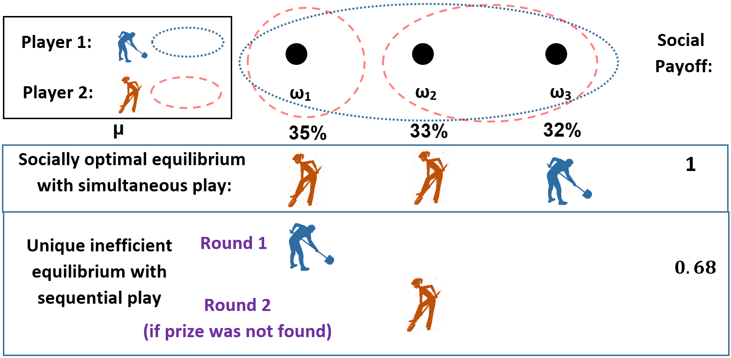
G=\left(N=\left\{1,2\right\},\Omega=\left\{\omega_{1},\omega_{2},\omega_{3}\right\},\Pi,\mu,K\equiv 1,c\equiv 0,\left(v_{i}^{1}\equiv 1,v_{i}^{2}\equiv 0.5,v_{\mathfrak{s}}\equiv 1\right)\right)

be a two-player search game with three locations, capacity 1 for each player and costless search. All locations yield a private value of 1, which is equally shared between simultaneous finders. Player 1 has the trivial partition $\Pi_{1}=\left\{\Omega\right\}$ , while Player $2$ knows if the prize is in location $\omega_{1}$ or not (i.e., $\Pi_{2}=\left\{\left\{\omega_{1}\right\},\left\{\omega_{2},\omega_{3}\right\}\right\}$ . The prior assigns slightly higher (resp., lower) probability to location $\omega_{1}$ (resp., $\omega_{3}$ ), i.e., $\mu\left(\omega_{1}\right)=35\%$ , $\mu\left(\omega_{2}\right)=33\%$ , $\mu\left(\omega_{3}\right)=32\%$ . Observe that the game satisfies ordinal consistency and solitary-search dominance. In our model, in which players search simultaneously, the game admits two (pure) Nash equilibria, both of which are socially optimal: Player 1 searches in either location 2 or 3, and Player 2 searches in the remaining two locations.

By contrast, if the game is sequential and Player 1 plays first, then the game admits a unique equilibrium, which is not efficient: Player 1 searches in $\omega_{1}$ , and if the prize has not been found, Player 2 searches in location $\omega_{2}$ (and no player searches in location $\omega_{3}$ ). Note that this profile is the unique equilibrium regardless of whether or not the model lets Player 2 observe the location in which Player 1 searched in the previous round.

3.4 Implications for Innovation Contests

Consider the setup of an innovation contest, in which a contest designer, who wishes to maximize the social payoff, might influence the private payoffs of players by offering a monetary bonus to the prize’s finder, which is added to the inherent reward. In what follows we sketch a few implications of Theorem 1 in a contest with asymmetric information, while leaving the interesting question of characterizing the optimal bonuses in this setup to future research.

Observe first that if the private payoffs satisfy ordinal consistency and solitary-search dominance, then Theorem 1 implies that the designer can maximize the social payoff without offering any bonus: the designer is only required to be able to give nonenforced recommendations to the players (which allows him to induce the play of the socially optimal Nash equilibrium, rather than other equilibria). In what follows we consider the case in which solitary-search dominance is violated in the search game (without additional monetary bonuses).

Consider first a setup in which the contest designer can only offer a constant bonus, which is independent of the prize’s location. A constant bonus can help to increase the relative expected private value of locations with a high prior probability. As a result, it can help obtain the optimal social payoff, when the reason for not having the required properties without the designer’s intervention is a low-prior location having a too-high private value. For example, consider a search game with costless search (i.e., $c\equiv 0$ ), where there are two locations $\omega,\omega^{\prime}$ in the same cell of player $i$ with priors $\mu\left(\omega\right)=0.1$ and $\mu\left(\omega^{\prime}\right)=0.2$ and with private values of $v_{i}^{1}\left(\omega\right)=5$ and $v_{i}^{1}\left(\omega^{\prime}\right)=1$ , and $v_{i}^{m}\equiv\frac{1}{m}v_{i}^{1}$ . The too-high private value of location $\omega$ violates solitary-search dominance because the expected private value in $\omega$ ( $0.5=0.1\cdot 5$ ) is more than twice the expected private value in $\omega^{\prime}$ ( $0.2\cdot 1$ ). A constant bonus of $1$ would restore solitary-search dominance (making the expected private value of $\omega$ and $\omega^{\prime}$ to be equal to $0.6=0.1\cdot\left(5+1\right)$ and $0.4=0.2\cdot\left(1+1\right)$ , respectively).

When the designer can offer a location-dependent and player-dependent bonus, it allows him to obtain solitary-search dominance and ordinal consistency when faced with any profile of rewards. An interesting open question is how the designer can maximize the social payoff, while minimizing the expected bonus. For example, assume that the payoffs are ordinally consistent, but they are not solitary-search dominant. Theorem 1 suggests that the designer should boost locations that have lower expected private values (which violate solitary-search dominance). Note that these locations might not coincide with the locations that are not searched by any player in the inefficient equilibrium. This is demonstrated in Example 4.

Example 4.

Consider the following search game with common values (as illustrated in Figure 4):

$\left(N=\left\{1,2\right\},\Omega=\left\{\omega_{1},\omega_{2},\omega_{3},\omega_{4}\right\},\Pi,\mu,K\equiv 1,c\equiv 0,v_{i}^{m}\equiv\frac{1}{m},v_{\mathfrak{s}}\equiv 1\right)$ , where the prior is $\mu\left(\omega_{1}\right)=44\%$ , $\mu\left(\omega_{2}\right)=21\%,$ $\mu\left(\omega_{3}\right)=20\%$ and $\mu\left(\omega_{4}\right)=15\%$ , player 1 observes whether the prize’s location is 1 or not, i.e., $\Pi_{1}=\left\{\left\{\omega_{1}\right\},\left\{\omega_{2},\omega_{3},\omega_{4}\right\}\right\}$ , and player 2 observes whether the prize’s location is at most 2 or not, i.e., $\Pi_{2}=\left\{\left\{\omega_{1},\omega_{2}\right\},\left\{\omega_{3},\omega_{4}\right\}\right\}$ . The game admits a unique equilibrium, in which player 1 searches in $\omega_{1}$ and $\omega_{2}$ , while player 2 searches in locations $\omega_{1}$ and $\omega_{3}$ . This equilibrium yields an expected social payoff of 0.85 because no player searches in $\omega_{4}$ . Note that solitary-search dominance is violated because of the low probability of location $\omega_{2}$ (rather than a low probability of $\omega_{4}$ ).

If the designer can offer a bonus of 0.05 that increases the private value in location $\omega_{2}$ by 5% to 1.05 (which requires a modest expected bonus of $21\%\cdot 0.05\approx 0.01$ ), then the modified rewards satisfy solitary-search dominance, and, as a result, the game admits a socially optimal equilibrium with a social payoff of 1 (in which player 1 searches in locations $\omega_{1}$ and $\omega_{4}$ , while player 2 searches in locations $\omega_{2}$ and $\omega_{3}$ ).

4 Socially Optimal Payoff

Theorem 1 has provided conditions under which the socially optimal (first-best) payoff is also yielded by some equilibrium. In this section we present lower bounds (which are binding in many cases, as demonstrated below) for the socially optimal payoff, namely, for the highest social payoff yielded by any strategy profile. Thus, we do not explicitly mention equilibria in this section; nevertheless, we remind the reader that by Theorem 1 the socially optimal payoff yielded in every result or example of this section is also yielded by some equilibrium of the game, if payoffs are ordinally consistent and solitary-search dominant.

Given a profile of strategies, society cares only about which locations are being searched (by anyone) and which are not. Define a pure outcome as a function $f:\Omega\rightarrow\left\{0,1\right\}$ that specifies which locations are being searched. A strategy profile induces a pure outcome, and, of course, not every outcome can be induced by strategies. Similarly, we define a mixed outcome as a function $f:\Omega\rightarrow\left[0,1\right]$ , where $f\left(\omega\right)$ is the probability that $\omega$ is being searched. A lottery over strategy profiles induces a mixed outcome. The notion of mixed outcomes turns out to be helpful for deriving and presenting our lower bounds for the socially optimal payoff, as demonstrated in the following example.

Example 5 (“Three coins”).

Consider a game where the locations $\Omega=\left\{0,1\right\}^{3}$ are vectors of three binary coordinates. Each player has a capacity of one, the social payoff $v_{\mathfrak{s}}\equiv 1$ is one in every location, and $\mu$ is uniform over $\Omega$ . There are three players, and player $i$ knows the $i$ -th coordinate of the prize’s location. Intuitively, this game can be interpreted as nature tossing three coins to determine the prize’s location, with each player observing the result of one of these coin tosses. Let $f$ be the mixed outcome that assigns $f\left(\omega\right)=3/4$ to every location $\omega$ . We will see that $f$ can be induced by a lottery over strategy profiles. This implies that the socially optimal payoff is at least $3/4$ .

Note that the socially optimal payoff in Example 5 cannot exceed $3/4$ . The reason is that for any strategy profile, the number of searched locations is at most the number of cells of all players (multiplied by the capacity), $\sum_{i\in N}\thinspace K_{i}\cdot\left|\Pi_{i}\right|$ , which is six in the example, while $\left|\Omega\right|=8$ . Similarly, for any subset of locations $W\subseteq\Omega$ , the number of searched locations within $W$ is at most the number of cells that intersect $W$ (namely, $\sum_{i\in N}K_{i}\cdot\left|\left\{\pi_{i}\in\Pi_{i}\right\}:\pi_{i}\cap W\neq\emptyset\right|$ ). Next, consider a mixed outcome $f$ induced by a lottery over strategy profiles. The mixed outcome must satisfy that the expected number of searched locations within $W$ (i.e., $\sum_{\omega\in W}f\left(\omega\right))$ is at most the number of cells that intersect $W$ ; that is, $f$ must satisfy the following compatibility property.

Definition 5.

A mixed outcome $f$ is compatible with the information structure (henceforth, compatible) if for any subset of locations $W\subseteq\Omega$ , the following inequality holds:

\sum_{\omega\in W}f\left(\omega\right)\leq\sum_{i\in N}K_{i}\cdot\left|\left\{\pi_{i}\in\Pi_{i}\right\}:\pi_{i}\cap W\neq\emptyset\right|\,\,.

(3)

We will later show that the opposite also holds; namely, any compatible outcome can be induced by a lottery over profiles. This will allow us to derive our first lower bound for the socially optimal payoff.

Let us now verify that $f$ of Example 5 is compatible. For any $W\subseteq\Omega$ , the LHS of (3) equals $3/4\cdot\left|W\right|$ . The partition of every player $i$ consists of two cells, each of size four. Therefore, the number of cells of player $i$ that intersect $W$ is at least $\left|W\right|/4$ ; hence, the RHS of (3) is at least $\sum_{i\in N}\left|W\right|/4=3/4\cdot\left|W\right|=\sum_{\omega\in W}f\left(\omega\right)$ .

We now define another class of outcomes, those that are generated by a fractional allocation, which will be helpful in deriving the second lower bound for the socially optimal payoff.

Definition 6.

A fractional allocation $\alpha=\left(\alpha_{1},\ldots,\alpha_{n}\right)$ specifies a nonnegative number $\alpha_{i}\left(\pi_{i},\omega\right)$ for every cell $\pi_{i}$ of player $i$ and every location $\omega\in\pi_{i}$ , such that $\sum_{\omega\in\pi_{i}}\,\alpha_{i}\left(\pi_{i},\omega\right)\leq K_{i}$ for any cell $\pi_{i}$ .
A fractional allocation generates the mixed outcome $f_{\alpha}$ that assigns to every location $\omega$ the sum of the allocations to $\omega$ over all players (as long as this sum does not exceed one). That is, $f_{\alpha}\left(\omega\right)=\min$ $\left(1,\,\sum_{i\in N}\thinspace\alpha_{i}\left(\pi_{i}(\omega),\omega\right)\,\right)$ .

Example 6.

Suppose that there are $n$ players, each with a capacity of one, and all cells are of the same size $m$ , where $m\geq n$ . Let $\alpha_{i}$ divide each player’s capacity equally between the locations within each cell, i.e., $\alpha_{i}\left(\pi_{i},\omega\right)=1/m$ for each cell $\pi_{i}$ and location $\omega\in\pi_{i}$ . Then this fractional allocation $\alpha=\left(\alpha_{1},\ldots,\alpha_{n}\right)$ generates the outcome $f\left(\omega\right)=n/m$ in every $\omega$ .

Suppose that each player in Example 6 independently employs a randomized strategy that chooses, within each cell, each location with equal probability $1/m$ . This is equivalent to a lottery over strategy profiles that gives equal probability to every pure profile that exhibits no idleness (i.e., every profile in which all players always use their entire search capacity). Search duplication occurs under some of these profiles, which implies that the induced outcome would be, in every $\omega$ , strictly less than $n/m$ . By contrast, in our definition of an outcome generated by a fractional allocation, the accumulation in every $\omega$ is done without any “waste.” Nevertheless, we now show that this wasteless outcome can always be achieved by a lottery over profiles.

The following proposition states that both classes of outcomes defined above coincide with the outcomes that can be induced by a lottery over profiles.

Proposition 2.

For a mixed outcome $f$ , the following conditions are equivalent:
(i) $f$ can be induced by a lottery over strategy profiles,
(ii) $f$ is compatible, and
(iii) $f$ can be generated by a fractional allocation.

Proposition 2 implies that the outcome $f\left(\omega\right)=3/4$ $\forall\omega$ in Example 5 is induced by some lottery over strategy profiles. This outcome yields a social payoff of $3/4$ and, hence, the support of the lottery must contain a profile that yields at least that much; therefore, the socially optimal payoff, $U_{\textrm{opt}}$ , is at least $3/4$ (and hence $U_{\textrm{opt}}=3/4$ ). Similarly, in Example 6 the outcome $f\left(\omega\right)=n/m$ $\forall\omega$ is induced by some lottery over profiles; therefore, the socially optimal payoff is at least $n/m\cdot\sum_{\omega\in\Omega\,}\mu\left(\omega\right)v_{\mathfrak{s}}\left(\omega\right)$ . Thus, in general, Proposition 2 implies the following two useful lower bounds for the socially optimal payoff.

Theorem 2.

(i) For any compatible outcome $f$ , the socially optimal payoff is at least the social payoff yielded by $f$ , i.e., $U_{\textrm{opt}}\geq\sum_{\omega\in\Omega\,}f\left(\omega\right)\cdot\mu\left(\omega\right)v_{\mathfrak{s}}\left(\omega\right)$ .
(ii) For any fractional allocation $\alpha$ , the socially optimal payoff is at least the social payoff yielded by the generated outcome, i.e., $U_{\textrm{opt}}\geq\sum_{\omega\in\Omega\,}f_{\alpha}\left(\omega\right)\cdot\mu\left(\omega\right)v_{\mathfrak{s}}\left(\omega\right)$ .

In addition, Proposition 2 implies the following characterization of the socially optimal payoff.

Corollary 3.

$U_{\textrm{opt}}=\max_{f\in F_{C}}\,\sum_{\omega\in\Omega\,}f\left(\omega\right)\cdot\mu\left(\omega\right)v_{\mathfrak{s}}\left(\omega\right)=\max_{f\in F_{F}}\,\sum_{\omega\in\Omega\,}f\left(\omega\right)\cdot\mu\left(\omega\right)v_{\mathfrak{s}}\left(\omega\right)$ , where $F_{C}$ denotes the set of compatible outcomes and $F_{F}$ denotes the set of outcomes generated by fractional allocations.

Sketch of proof of Proposition 2; formal proof in Appendix B.

We already explained why (i) $\Rightarrow$ (ii). To see that (ii) $\Rightarrow$ (iii), we construct a flow network: a directed graph whose edges have flow capacities. The graph connects every cell to the locations contained in it, with infinite flow capacity (as illustrated in Figure 5). We add a source vertex that connects to every cell, with flow capacity $K_{i}$ , and a sink vertex to which every location $\omega$ is connected, with flow capacity $f(\omega)$ . A cut is a subset of edges without which there exists no path from the source to the sink. The compatibility of $f$ implies that the minimal cut has a total capacity of $\sum_{\omega\in\Omega}f\left(\omega\right).$ Therefore, by the max-flow min-cut theorem (Ford and Fulkerson 1956; see a textbook presentation in Cormen et al. 2009, p. 723, Thm. 26.6), the network admits a flow of $\sum_{\omega\in\Omega}f\left(\omega\right).$ We define a fractional allocation $\alpha$ that generates $f$ by letting ${\color[rgb]{0,0,0}\alpha}_{i}\left(\pi_{i},\omega\right)$ equal the flow from $\pi_{i}$ to $\omega$ .

Now we show that (iii) $\Rightarrow$ (i). To simplify the sketch of the proof assume that all capacities are equal to one. Let $\alpha$ be a fractional allocation. We can represent $\alpha$ as a matrix $\left(A_{\pi\omega}^{{\color[rgb]{0,0,0}\alpha}}\right)_{\omega\in\Omega,\pi\,\textrm{is\,a\,cell}}\,$ , where

A_{\pi\omega}^{{\color[rgb]{0,0,0}\alpha}}=\begin{cases}{\color[rgb]{0,0,0}\alpha_{i}}\left(\pi,\omega\right)&\omega\in\pi,\,\pi\in\Pi_{i}\\ 0&\textrm{elsewhere\,.}\end{cases}

Observe that $A_{\pi\omega}^{{\color[rgb]{0,0,0}\alpha}}$ is a nonnegative matrix, and that the sum of each row $\pi$ is at most one. Let $B_{\pi\omega}^{{\color[rgb]{0,0,0}\alpha}}$ be a matrix derived from $A_{\pi\omega}^{{\color[rgb]{0,0,0}\alpha}}$ by decreasing elements of the matrix such that the sum of each column $\omega$ that exceeded one in $A_{\pi\omega}^{{\color[rgb]{0,0,0}\alpha}}$ is equal to one in $B_{\pi\omega}^{{\color[rgb]{0,0,0}\alpha}}$ . Observe that $B_{\pi\omega}^{{\color[rgb]{0,0,0}\alpha}}$ is a doubly substochastic matrix; i.e., it is a nonnegative matrix for which the sum of each column and each row is at most one. A simple adaptation of the Birkhoff–von Neumann theorem shows that $B_{\pi\omega}^{{\color[rgb]{0,0,0}\alpha}}$ can be represented as a convex combination of matrices $C_{\pi\omega}^{1},...,C_{\pi\omega}^{K}$ (i.e., $B_{\pi\omega}^{{\color[rgb]{0,0,0}\alpha}}=\sum w_{k}\cdot C_{\pi\omega}^{k}$ where $\sum w_{k}=1$ and $w_{k}\geq 0$ ), where each matrix $C_{\pi\omega}^{k}$ : (1) contains only zeros and ones, and (2) contains in each row and in each column at most a single value of one. Observe that each such matrix $C_{\pi\omega}^{k}$ corresponds to a pure profile $s^{k}$ in the search game, and that the outcome $f_{{\color[rgb]{0,0,0}\alpha}}$ is a weighted sum of the outcomes induced by the profiles $s^{k}$ . This implies that $f_{{\color[rgb]{0,0,0}\alpha}}$ is induced by the lottery over strategy profiles $\sigma=\sum w_{k}\cdot s^{k}$ . ∎

Next, we present two examples that demonstrate the usefulness of the lower bounds of Theorem 2. The first example extends Example 6.

Example 6 (revisited).

In Example 6 we had $n$ players and cells of uniform size $m\geq n$ . In particular, if $m=n$ then we get that $f\left(\omega\right)=n/m=1$ in every location. This implies that the game admits an exhaustive strategy profile, i.e., $U_{\textrm{opt}}=\sum_{\omega\in\Omega\,}\mu\left(\omega\right)v_{\mathfrak{s}}\left(\omega\right)$ . Likewise, if $m<n$ then the game admits an exhaustive profile, since $f\left(\omega\right)=\min\left(1,\,n/m\right)=1.$

More generally, when the capacity $K_{i}$ of each player $i$ is not necessarily one and the cells are not of uniform size, let $M_{i}$ denote the size of the largest cell of player $i$ . Then $f\left(\omega\right)\geq\min\left(1,\,\sum_{i\in N}\nicefrac{{K_{i}}}{{M_{i}}}\right)$ and $U_{\textrm{opt}}\geq\min\left(1,\,\sum_{i\in N}\nicefrac{{K_{i}}}{{M_{i}}}\right)\cdot\sum_{\omega\in\Omega\,}\mu\left(\omega\right)v_{\mathfrak{s}}\left(\omega\right)$ . In particular, if $\sum_{i\in N}\nicefrac{{K_{i}}}{{M_{i}}}\geq 1$ then the game admits an exhaustive strategy profile.⁹⁹ 9 By a similar argument, let $m_{i}=\min\left(\left|\pi_{i}\right|:\pi_{i}\in\Pi_{i}\right)$ ; then, if $\sum_{i\in N}\nicefrac{{K_{i}}}{{m_{i}}}\leq 1$ then the game admits a profile that always employs full capacity, while avoiding search duplication (see also Definition 8 in Section 5).

We conclude this section with an example in which a compatible outcome allows us to find the socially optimal payoff.

Example 7.

Suppose that $\Omega$ contains ten vectors, each of four binary coordinates, i.e., $\Omega\subset\left\{0,1\right\}^{4}$ and $\left|\Omega\right|=10$ . There are four players, each of capacity one, and player $i$ knows the $i$ -th coordinate. Let us show that the outcome that assigns $f\left(\omega\right)=0.8$ to every $\omega$ is compatible. Let $W\subseteq\Omega$ , and suppose first that all eight cells intersect $W$ . Then, since $\sum_{\omega\in W}\thinspace f\left(\omega\right)\leq\sum_{\omega\in\Omega}\thinspace f\left(\omega\right)=8,$ inequality (3) holds. Now, a cell of player $i$ does not intersect $W$ if every $\omega\in W$ resides in the other cell of player $i$ ; i.e., the $i$ -th coordinate is fixed across $W$ . Suppose that $k$ cells in all do not intersect $W$ , $1\leq k\leq 4$ . Then there are only $4-k$ “free” coordinates, therefore, $\left|W\right|\leq 2^{4-k}$ , and hence $\sum_{\omega\in W}\thinspace f\left(\omega\right)\leq 0.8\cdot 2^{4-k}$ . Let us verify that this is less than the number of cells that do intersect $W$ , i.e., that $0.8\cdot 2^{4-k}\leq 8-k$ . Indeed, for $k=1$ the LHS is $6.4$ and the RHS is $7$ , and for larger $k$ the difference increases.

Since $f$ is compatible, if the social payoff is one in every location and $\mu$ is uniform, then $U_{\textrm{opt}}=0.8$ . Put differently, there are eight cells (and thus at most eight locations can be searched); and the compatibility of $f$ implies the existence of a strategy profile under which eight locations are searched.

Note that if $\Omega$ happens to have exactly five zeros and five ones on each coordinate, then the fractional allocation that divides equally within every cell generates the above outcome $f$ . If $\Omega$ does not have this property, then identifying a fractional allocation that generates $f$ might be somewhat difficult; nevertheless, Proposition 2 tells us that such an allocation does exist.

5 Cost-Inclusive Social Payoff

In this subsection we consider a variant of our model, in which society internalizes the players’ search costs. We examine conditions under which the game admits a socially optimal equilibrium, as in Theorem 1.

We define the cost-inclusive social payoff, conditional on the prize’s location being $\omega$ , as

U_{CI}\left(s|\omega\right)=v_{\mathfrak{s}}\left(\omega\right)\cdot\boldsymbol{1}_{m_{s}\left(\omega\right)\geq 1}-\sum_{i\in N}c_{i}\left(\left|s_{i}\left(\pi_{i}\left(\omega\right)\right)\right|\right),

and the expected cost-inclusive social payoff is $U_{CI}\left(s\right)=\sum_{\omega\in\Omega}\,\mu\left(\omega\right)\cdot U_{CI}\left(s|\omega\right)$ .

First, note that in the baseline model, in which society disregards the players’ costs, society always prefers player $i$ searching an unoccupied location to player $i$ not searching. But here, with the cost-inclusive social payoff, this may no longer be true. Thus, the preference of an individual player $i$ who wishes to search despite her cost (by the second part of the solitary-search dominance definition) may diverge from society’s preference, as society may wish player $i$ to be idle. Hence, we add here the following assumption, which says that the expected social value always exceeds any expected marginal cost.

Definition 7.

We say that social value outweighs cost if

\mu\left(\omega\right)\cdot v_{\mathfrak{s}}\left(\omega\right)\geq\mu\left(\pi_{i}\right)\cdot\left(c_{i}\left(K_{i}\right)-c_{i}\left(K_{i}-1\right)\right)

for any location $\omega$ , player $i$ , and cell $\pi_{i}$ .

Nevertheless, even under the assumption that social value outweighs cost, on top of the assumptions of ordinal consistency and solitary-search dominance in Theorem 1, the game still need not admit a socially optimal equilibrium, as the following simple example demonstrates.

Example 8.

Let $G=\left(N=\left\{1,2\right\},\Omega=\left\{\omega\right\},\Pi,\mu,K\equiv 1,c\equiv 0.1,v_{i}^{m}\equiv\frac{`1}{m},v_{\mathfrak{s}}\equiv 1\right)$ be a game with two players and a single location $\omega$ . The dominant action of each player is to search $\omega$ ; hence, both players searching $\omega$ is the unique equilibrium, and this equilibrium is not socially optimal (since in any cost-inclusive socially optimal profile, only one player searches in $\omega$ ).

The players in the above example “step on each other’s toes” because the information structure does not allow them to each search in a separate location. We now show that the game does admit a socially optimal equilibrium if we assume, in addition, that the information structure is spacious enough; more precisely, if we assume that the information structure allows the existence of at least one redundancy-free strategy profile, namely, a profile under which players utilize their full search capacity and no two players search in the same location.

Definition 8.

A strategy profile $s$ is redundancy-free if (1) every player always uses her entire capacity (i.e., $\left|s_{i}\left(\pi_{i}\right)\right|=K_{i}$ for every cell $\pi_{i}$ of every player $i$ ), and (2) there is no search duplication (i.e., $m_{s}\left(\omega\right)\leq 1$ for every $\omega\in\Omega$ ).

Proposition 3.

Suppose that payoffs are ordinally consistent and solitary-search dominant, social value outweighs cost, and there exists a redundancy-free strategy profile. Then the game admits a (cost-inclusive) socially optimal pure equilibrium.

Sketch of proof; formal proof is in Appendix C.

Let $s^{{\scriptscriptstyle 1}}$ be a redundancy-free profile. Let $s^{{\scriptscriptstyle 2}}$ be a (cost-inclusive) socially optimal profile, and let $W$ denote the locations that are searched (by anyone) under $s^{{\scriptscriptstyle 2}}$ . Start with $s^{{\scriptscriptstyle 1}}$ ; suppose that there is a location $w\in W$ that is currently not being searched, then switch the player who searched $w$ under $s^{{\scriptscriptstyle 2}}$ from one of her current locations to $w$ . We repeat this step until we get a profile $s$ under which the whole $W$ is searched, while $s$ is still redundancy-free.

First, we demonstrate that $s$ is socially optimal, by comparing it to $s^{{\scriptscriptstyle 2}}$ . If there are locations outside $W$ that are searched under $s$ , then, by our assumption that social value outweighs cost, the expected social payoff yielded by $s$ is at least as high as that yielded by $s^{{\scriptscriptstyle 2}}$ (i.e., the additional social value of these locations exceeds the additional cost). Next, starting from $s$ , consider the improvement path of Proposition 1 that ends in an equilibrium. Since $s$ is redundancy-free, solitary-search dominance implies that, along this path, no player switches either to searching an occupied location or to being idle. A switch to an unoccupied location that improves a player’s payoff does not decrease the social payoff, by ordinal consistency. Therefore, since $s$ is socially optimal, so is the final equilibrium. ∎

Remark 2.

Adding information to a player, i.e., refining her information partition, always weakly increases the socially optimal payoff. Note, however, that if we begin with an information structure that admits a redundancy-free profile and then we refine some partitions, the structure becomes more crowded, and we could end up with a structure that does not admit a redundancy-free profile and, therefore, the new socially optimal payoff may not be achieved by an equilibrium.

If there is no redundancy-free profile, then the existence of a socially optimal equilibrium is still guaranteed if, in addition to the other assumptions of Proposition 3, the expected reward in any location is smaller, when the reward is shared with others, than any marginal cost. The proof, then, is similar to that of Theorem 1.

6 Conclusion

Our paper studies search games in which agents explore different routes to making a discovery that would benefit both society and the discoverer (although the private gain may differ from the social gain). Our main departure from the related literature is that we introduce asymmetric information to this setup. That is, we allow each agent to have private information about the plausibility of different routes, while almost all of the existing literature assumes that all agents have the same information. We believe that this is a natural development, as asymmetric information is a key component in many real-life decentralized research situations. In addition, we allow substantial heterogeneity between the different routes (i.e., different expected values of finding the prize in different locations). We also allow heterogeneity in the rewards and costs of different players.

Our model is simplified in one aspect, as we assume that the search is a one-shot game, while the dynamic aspects of the search interaction are a key component in many of the existing models (see, e.g., Chatterjee and Evans 2004; Akcigit and Liu 2015; Bryan and Lemus 2017). While a one-shot game might model reasonably well situations with severe time constraints, such as the motivating example of developing a COVID-19 vaccine as soon as possible, we think that incorporating asymmetric information in a dynamic search game is an important avenue for future research.

Our first main result (Theorem 1) states that a search game admits a (pure) equilibrium that yields the first-best social payoff if for any two locations within a player’s cell: (1) the player and society have the same ordinal ranking over these two locations (ordinal consistency), and (2) the player always prefers searching in one of these locations alone to searching in the other location with other players, or to not searching at all (solitary-search dominance). Taylor 1995; Fullerton and McAfee 1999; Che and Gale 2003; Koh 2017 present setups of innovation contests in which it is socially optimal to restrict the number of participating players, because adding a player decreases the incentive of others to exert costly effort. By contrast, Theorem 1 implies that adding players to a search game with ordinally consistent and solitary-search dominant payoffs always improves the maximal social payoff that can be yielded by an equilibrium. This is so because the first-best social payoff is (weakly) increasing when players are added. Thus, when the payoffs are ordinally consistent and solitary-search dominant, it is socially optimal to allow all players to participate. It is an open question whether this property holds in our setup when we relax the assumptions of ordinal consistency and solitary-search dominance.

Our second main result provides useful, and often binding, lower bounds for the first-best payoff, whether it is achievable by an equilibrium or not. These bounds are established by showing that the outcomes that can be induced by a lottery over strategy profiles coincide with the compatible outcomes and with the outcomes that can be generated by a fractional allocation.

Appendix: Formal Proofs

Appendix A Proof of Prop. 1 (Search Games are Weakly Acyclic)

Given a strategy profile $s$ , we define, for any cell $\pi_{i}\in\Pi_{i}$ of player $i$ , the payoff of $\pi_{i}$ as the (interim) expected payoff of player $i$ given that her signal is $\pi_{i}$ , i.e., $u_{i}\left(s|\pi_{i}\right)=\sum_{\omega\in\pi_{i}}\,\mu\left(\omega|\pi_{i}\right)u_{i}\left(s|\omega\right)$ . Note that player $i$ is best-responding iff every cell of hers is best-responding.

Player $i$ has $K_{i}$ units of capacity, which we index by numbers between $1$ and $K_{i}$ . A cell-unit of player $i$ is a pair $\left(\pi_{i},j\right)$ where $\pi_{i}\in\Pi_{i}$ is a cell, and $1\leq j\leq K_{i}$ is a unit index. We can assume w.l.o.g. that a strategy specifies not only in which locations within $\pi_{i}$ to search, but also which specific cell-unit is assigned to each of these locations. Thus, for every cell-unit $\alpha$ of $i$ , a strategy of $i$ chooses a location or chooses that $\alpha$ be inactive. We can think of a player as being composed of many “smaller” decision makers, one for each cell of hers, and of each cell as being composed of even smaller decision makers, one for every cell-unit of that cell (with the restriction that two cell-units of the same cell cannot search in the same location). We define the payoff of cell-unit $\alpha=\left(\pi_{i},j\right)$ of player $i$ as the payoff of its cell $u_{i}\left(s|\pi_{i}\right)$ . Thus, every cell-unit of $\pi_{i}$ gets the same payoff. Note that the expected reward of a cell-unit located at $\omega$ is $\mu\left(\omega|\pi_{i}\right)\cdot v_{i}^{m_{s}\left(\omega\right)}\left(\omega\right)$ , and $u_{i}\left(s|\pi_{i}\right)$ equals the sum of the expected rewards of the active cell-units of $\pi_{i}$ minus the cost $c_{i}$ of the number of active cell-units of $\pi_{i}$ .

Observe that if an inactive cell-unit $\left(\pi_{i},j\right)$ switches to searching in location $\omega$ , it makes the activation of another cell-unit $\left(\pi_{i},j^{\prime}\right)$ at $\omega^{\prime}$ (weakly) less attractive than it previously was, because of increasing marginal costs (namely, the convexity of costs). Similarly, deactivating a cell-unit makes a second deactivation weakly less attractive.

Given a strategy profile $s$ , if there exists a deviation of a single cell-unit that improves its own payoff then, by definition, it is also an improvement for its cell. Conversely, let us show that the existence of an improvement for a cell implies the existence of an improvement for some cell-unit. Suppose first that the cell improvement consists merely of changing the location of a few cell-units, without changing the number of active units. Then the cost remains unchanged, but the overall expected reward has increased. Hence, there must be at least one cell-unit $\alpha$ whose expected reward has increased by switching from its location $\omega$ to another location $\omega^{\prime}$ that was not chosen by player $i$ under $s$ . Therefore, switching the location of $\alpha$ from $\omega$ to $\omega^{\prime}$ is an improvement for $\alpha$ . Next, suppose that activating multiple cell-units is an improvement. Then there must also exist an improvement consisting of activating only one of these cell-units, due to the above observation about convex costs. Similarly, if the cell can improve by deactivating multiple cell-units then one of them can improve by deactivating itself.

Overall, we got that a player is best-responding iff all her cells are best-responding iff all her cell-units are best-responding.

Lemma 1.

Suppose that $B$ is a set of cell-units (of various players), $\alpha\notin B$ is another cell-unit, and $s^{{\scriptscriptstyle 1}}$ is a strategy profile under which every member of $B$ is best-responding. Then there exists a finite sequence of cell-unit improvements $s^{{\scriptscriptstyle 1}},\ldots,s^{{\scriptscriptstyle T}}$ such that every member of $B\cup\{\alpha\}$ is best-responding under $s^{{\scriptscriptstyle T}}$ .

Proof.

For convenience of description, let us imagine that all the inactive cell-unit of all players stay in some place that we denote by $\lambda$ . The set $\Omega\cup\left\{\lambda\right\}$ of the locations plus $\lambda$ will be called the set of sites. With this terminology, we can say that a strategy of player $i$ chooses a site for every cell-unit of $i$ (and $\lambda$ is the only site where more than one cell-unit of the same player can be placed).

In what follows, whenever we mention cell-units, it only refers to members of $B\cup\{\alpha\}$ . Note that the site of all other cell-units will remain fixed along the sequence.

Suppose that $\alpha$ is not best-responding in $s^{{\scriptscriptstyle 1}}$ ; otherwise we are done. Let $\alpha$ switch from its current site $\theta^{1}$ to another site $\theta^{2}$ that is a best-response. The new strategy profile is $s^{{\scriptscriptstyle 2}}$ . Now $\alpha$ is best-responding, and we claim that any other cell-unit $\beta$ of the same cell is still best-responding. We note first that $\beta$ is not placed in $\theta^{1}$ (since $\beta$ was best-responding under $s^{{\scriptscriptstyle 1}}$ ), and w.l.o.g. it is also not in $\theta^{2}$ (otherwise, it is currently best-responding, since $\alpha$ is). Next we note that $\beta$ cannot improve by switching to $\theta^{1}$ ; otherwise, simply switching $\beta$ to $\theta^{2}$ would have been an improvement earlier, in $s^{{\scriptscriptstyle 1}}$ .

Suppose first that $\theta^{1}$ and $\theta^{2}$ are both locations. Then, since $\theta^{2}$ is now occupied, and the preference relation between sites other than $\theta^{1}$ and $\theta^{2}$ has not changed (as the cost has not changed), $\beta$ is indeed still best-responding. Next suppose that $\theta^{2}=\lambda$ . Then, by the convex costs observation, the attractiveness of $\lambda$ has decreased by the switch from $\theta^{1}$ to $\theta^{2}=\lambda$ , hence $\beta$ still cannot improve by switching to $\lambda$ . And although the cost has changed, the relation between locations other than $\theta^{1}$ has not changed; hence, $\beta$ is best-responding. Finally, suppose that $\theta^{1}=\lambda$ . Then the relation between locations other than $\theta^{2}$ has not changed; hence, $\beta$ is best-responding.

Phase I

In $s^{{\scriptscriptstyle 2}}$ , we add a dummy player at the site $\theta^{1}$ , denoting the resulting strategy profile by $\sigma^{{\scriptscriptstyle 2}}$ (for a profile $\sigma^{t}$ that includes the dummy player, $s^{t}$ will denote the same profile without the dummy). Then Phase I begins: at every stage of Phase I, one cell-unit who is currently not best-responding switches to a best-response site. This continues as long as there are non-best-responding cell-units, unless someone switches to $\theta^{1}$ , in which case Phase I immediately terminates.

As we will see, Phase I begins by some cell-unit switching from $\theta^{2}$ to another site $\theta^{3}$ , then another cell-unit switching from $\theta^{3}$ to another site, etc. More specifically, we claim that under any strategy profile $\sigma=\sigma^{t}$ encountered during Phase I,

(a) there exists exactly one site $\theta$ that is chosen by one more cell-unit than under $s^{{\scriptscriptstyle 1}}$ , i.e., $m_{\sigma}(\theta)=m_{s^{{\scriptscriptstyle 1}}}(\theta)+1$ , while for every other site $\theta^{\prime}$ , $m_{\sigma}(\theta^{\prime})=m_{s^{{\scriptscriptstyle 1}}}(\theta^{\prime})$ (we call $\theta$ “the plus site”); and

(b) for any cell-unit $\beta$ whose current site is some $\theta$ with $m_{\sigma}(\theta)>0$ , and who can also choose another site $\theta^{\prime}$ , if there were $m_{s^{{\scriptscriptstyle 1}}}(\theta)$ cell-units at $\theta$ (including $\beta$ itself) and $m_{s^{{\scriptscriptstyle 1}}}(\theta^{\prime})$ cell-units at $\theta^{\prime}$ , then $\beta$ would weakly prefer $\theta$ to $\theta^{\prime}$ .

Property (b) roughly says that if $\beta$ is not best-responding, it is only because $\beta$ is in the plus site.

When Phase I starts, in $\sigma^{{\scriptscriptstyle 2}}$ , property (a) holds and $\alpha$ has just switched to the plus site $\theta^{2}$ . Since all cell-units of the cell of $\alpha$ were best-responding in $s^{{\scriptscriptstyle 2}}$ (i.e., without the dummy) they obey property (b) in $\sigma^{{\scriptscriptstyle 2}}$ (in particular, $\alpha$ is currently best-responding when $\alpha$ ’s current site is the plus site, let alone when it is not the plus site). As for cell-units of other cells, they obeyed (b) in $s^{{\scriptscriptstyle 1}}$ and, therefore, they still do, as the switch of $\alpha$ or the addition of the dummy do not affect that.

The claim is proved by induction from one stage to the next: suppose that cell-unit $\beta$ improves on stage $t$ by switching from $\theta$ to $\theta^{\prime}$ . Since $\beta$ could improve, (b) implies that $\theta$ must have been the plus site in stage $t$ . Therefore, the plus will move with $\beta$ from $\theta$ to $\theta^{\prime}$ , and (a) will still hold in stage $t+1$ . Note that, importantly, if the plus site is $\lambda$ in some stage then every cell-unit is best-responding, since the number of partners does not affect the reward in $\lambda$ , which simply equals $0$ ; hence, Phase I will end on that stage.

As for property (b), $\beta$ best-responds in $\theta^{\prime}$ , and other cell-units of $\beta$ ’s cell obeyed (b) on stage $t$ , implying that they were best-responding on that stage. It follows, by the same argument we used above for $t=1$ (i.e., the transition from $s^{{\scriptscriptstyle 1}}$ to $s^{{\scriptscriptstyle 2}}$ ), that they also best-respond on stage $t+1$ . Therefore, they obey (b); and cell-units of other cells still obey (b), as they were not affected by $\beta$ ’s switch.

To see that Phase I cannot go on forever, recall first that it ends if the plus site is $\lambda$ . Otherwise, on each stage of Phase I some cell-unit $\beta$ switches from location $\omega$ to location $\omega^{\prime}$ , and the costs always remain fixed. Since this switch is an improvement, it strictly increases the expected reward of $\beta$ . Now $\omega^{\prime}$ becomes the plus site, and afterwards the expected reward of $\beta$ when placed in $\omega^{\prime}$ can never be lower than it is now, while it can be higher if the plus is somewhere else (or if $\beta$ improves again).¹⁰¹⁰ 10 One can verify that, in fact, $\beta$ will not switch again during Phase I. We employ a different argument here, in order to strengthen the analogy with Phase II. Thus, the expected reward of $\beta$ will never go down to the level it was at before the switch. Hence, Phase I cannot turn into a cycle, and since there are only finitely many strategy profiles, Phase I must eventually end.

Recall that Phase I terminates once someone switches to $\theta^{1}$ . Therefore, the plus site cannot be $\theta^{1}$ during this phase except maybe at the end, and hence nobody switches from $\theta^{1}$ during Phase I. Therefore, all the switches are improvements not only in the game with the dummy added at $\theta^{1}$ , but also in the original game.

Denote the strategy profile at the end of Phase I by $\sigma^{*}$ . Now we remove the dummy from $\theta^{1}.$ Suppose first that Phase I ended because somebody has just switched to $\theta^{1}$ . Then, the removal of the dummy means that now there is no plus site at all, and (b) implies that every cell-unit best-responds under $s^{*}$ (recall that $s^{*}$ is $\sigma^{*}$ without the dummy player), and we are done.

Phase II

Otherwise, Phase I ended at $\sigma^{*}$ because everyone was best-responding (when the dummy was still at $\theta^{1}$ ). Starting from $s^{*}$ , we define Phase II analogously to Phase I (while Phase I more or less described a process of restabilizing the system after one cell-unit is added, Phase II describes restabilizing it after one cell-unit is removed), as follows. At every stage, as long as there are cell-units who are not best-responding, choose a cell, and choose a switch of a single cell-unit that would yield the highest increase in that cell’s payoff.

As we will see, Phase II begins by some cell-unit switching to $\theta^{1}$ from some site $\theta^{\prime}$ , then another cell-unit switching to $\theta^{\prime}$ from another site, etc. More specifically, we claim that under any strategy profile $s=s^{t}$ encountered during Phase II,

(a’) there exists exactly one site $\theta$ with $m_{s}(\theta)=m_{\sigma^{*}}(\theta)-1$ , while for every other site $\theta^{\prime}$ , $m_{s}(\theta^{\prime})=\hat{m}_{\sigma^{*}}(\theta^{\prime})$ (we call $\theta$ “the minus site”); and

(b’) for any cell-unit $\beta$ whose current site is some $\theta$ and who can also choose site $\theta^{\prime}$ , if there were $m_{\sigma^{*}}(\theta)$ cell-units at $\theta$ (including $\beta$ ) and $m_{\sigma^{*}}(\theta^{\prime})$ cell-units at $\theta^{\prime}$ , then $\beta$ would weakly prefer $\theta$ to $\theta^{\prime}$ .

The analysis is almost analogous to that of Phase I. When Phase II starts, in the profile $s^{*}$ , (a’) holds and $\theta^{1}$ is the minus site. (b’) also holds because everyone was best-responding under $\sigma^{*}$ . The claim is proved by induction from one stage to the next: suppose that cell-unit $\beta$ improves on stage $t$ by switching from $\theta$ to $\theta^{\prime}$ . Improvement implies, by (b’), that $\theta^{\prime}$ must have been the minus site in stage $t$ . Therefore, the minus will move from $\theta^{\prime}$ to $\theta$ , and (a’) will still hold in stage $t+1$ . Note that if the minus site is $\lambda$ in some stage, then every cell-unit is best-responding and Phase II will end on that stage.

Let $\pi_{i}$ be the cell of $\beta$ . Any cell-unit of another cell still obeys (b’), as it was not affected by $\beta$ ’s switch. Since the switch of $\beta$ from $\theta$ to $\theta^{\prime}$ was, by definition of Phase II, a best cell-unit switch for $\pi_{i}$ , $\beta$ cannot improve again. Therefore, $\beta$ obeys (b’), since $\beta$ is not in the minus site. Let $\gamma$ be another cell-unit of $\pi_{i}$ . Note first that $\gamma$ cannot improve by switching to the current minus site $\theta$ ; otherwise, switching $\gamma$ to $\theta^{\prime}$ earlier, on stage $t$ , would have been a better switch than the one chosen.

We have seen that $\theta^{\prime}\neq\lambda$ . If also $\theta\neq\lambda$ , then the preference relation between sites other than $\theta$ and $\theta^{\prime}$ has not changed, and, therefore, $\gamma$ still obeys (b’). Otherwise, $\theta=\lambda$ . Then if $\gamma$ is placed in $\lambda$ it still obeys (b’), because the attractiveness of $\lambda$ has increased, by the convex costs observation; and if $\gamma$ is placed in some location then $\gamma$ still obeys (b’), because the relation between locations other than $\theta^{\prime}$ has not changed.

When Phase II ends, every cell-unit will be best-responding. To see that Phase II must eventually end, we employ the same argument as in Phase I, noting that right after some cell-unit $\beta$ switches to location $\omega^{\prime}$ , $\omega^{\prime}$ is not the minus site, and, therefore, the expected reward of $\beta$ when placed in $\omega^{\prime}$ can never be lower than it is now. ∎ To prove weak acyclicity, start from any strategy profile. By applying Lemma 1 inductively we obtain a sequence of cell-unit improvements that lead to a profile under which one cell-unit is best-responding, then two, and so on. Eventually we get a profile under which every cell-unit is best-responding, hence an equilibrium.

Appendix B Proof of Prop. 2 (3 Equivalent Classes of Outcomes)

We already explained why (i) $\Rightarrow$ (ii), right before Definition 5. To see that (ii) $\Rightarrow$ (iii), suppose $f$ is compatible. Denote the set of all cells of the search game by $\hat{\Pi}=\{(i;\pi_{i}):i\in N,\pi_{i}\in\Pi_{i}\}$ . We construct a flow network, namely, a directed graph $D=(V,E)$ with vertices $V$ and edges $E\subset V\times V$ , and a flow capacity $\kappa(v_{{\scriptscriptstyle 1}},v_{{\scriptscriptstyle 2}})\geq 0$ for every edge $(v_{{\scriptscriptstyle 1}},v_{{\scriptscriptstyle 2}})$ (illustrated beside the sketch of this proof, in Figure 5). There are two special vertices, a source $s$ and a sink $t$ . The other vertices in our network are the locations $\Omega$ and the cells $\hat{\Pi}$ of the game. There is an edge from $s$ to every $(i;\pi_{i})\in\hat{\Pi}$ , where $\kappa(s,(i;\pi_{i}))=K_{i}$ , and an edge from every location $\omega\in\Omega$ to $t$ , where $\kappa(\omega,t)=f(\omega)$ . Also, there is an edge from a cell $(i;\pi_{i})\in\hat{\Pi}$ to a location $\omega$ iff $\pi_{i}$ contains $\omega$ , and the flow capacity $\kappa$ of such edges is infinite (for a textbook presentation of flow networks; see, e.g., Cormen et al. 2009, Ch. 26).

A cut of $D$ is a subset of edges $C\subset E$ , such that if all the edges of $C$ are removed then there exists no path between $s$ and $t$ . Suppose that $C$ is a minimal cut, i.e., a cut whose sum of capacities is minimal. Then $C$ certainly does not include any edge between a cell and a location, as those edges have an infinite flow capacity. Let $Q=\left\{\omega\in\Omega:\left(\omega,t\right)\in C\right\}$ denote the locations that the cut separates from $t$ . Denote $W=\Omega\setminus Q$ . Then $C$ must include all the edges $\{(s,(i;\pi_{i})):i\in N,\pi_{i}\cap W\neq\emptyset\}$ ; otherwise there would still exist a path from $s$ to $t$ . Hence, the total capacity of $C$ equals

\sum_{\omega\in Q}\kappa\left(\omega,t\right)+\sum_{i\in N}\sum_{\pi_{i}\cap W\neq\emptyset}\kappa\left(s,\left(i;\pi_{i}\right)\right)=\sum_{\omega\in Q}f(\omega)+\sum_{i\in N}\sum_{\pi_{i}\cap W\neq\emptyset}K_{i}=

\sum_{\omega\in Q}f(\omega)+\sum_{i\in N}K_{i}\cdot\left|\left\{\pi_{i}\in\Pi_{i}:\pi_{i}\cap W\neq\emptyset\right\}\right|\geq\sum_{\omega\in Q}f(\omega)+\sum_{\omega\in W}f(\omega)=\sum_{\omega\in\Omega}f(\omega).

Therefore, the cut that consists of all edges of type $(\omega,t)$ , whose total capacity equals $\sum_{\omega\in\Omega}f(\omega)$ , is minimal.

A flow in $D$ is a function $\varphi:E\to\mathbb{{R}}^{+}$ such that: (i) the flow never exceeds the capacity, i.e., $\varphi(e)\leq\kappa(e)$ , and (ii) the overall flow outgoing from $s$ , namely, the sum of flows on edges outgoing from $s$ , equals the overall flow incoming to $t$ , namely, the sum of flows on edges incoming to $t$ (call this quantity the value of the flow), and for any other vertex the incoming flow equals the outgoing flow. The max-flow min-cut theorem (Cormen et al. 2009, p. 723, Theorem 26.6) states that the value of the maximal flow equals the total capacity of the minimal cut; therefore, $D$ admits a flow $\varphi$ of value $\sum_{\omega\in\Omega}f(\omega)$ , and so it must be the case that $\varphi(\omega,t)=f(\omega)$ for every $\omega\in\Omega$ .

Now define a fractional allocation $\alpha$ by letting ${\color[rgb]{0,0,0}\alpha}_{i}(\pi_{i},\omega)=\varphi((i;\pi_{i}),\omega)$ for every $i\in N$ , $\pi_{i}\in\Pi_{i}$ , and $\omega\in\pi_{i}$ . To see that this is a fractional allocation we verify that for any $\pi_{i}$ , $\sum_{\omega\in\pi_{i}}{\color[rgb]{0,0,0}\alpha}_{i}\left(\pi_{i},\omega\right)=\sum_{\omega\in\pi_{i}}\varphi((i;\pi_{i}),\omega)=\varphi(s,(i;\pi_{i}))\leq\kappa(s,(i;\pi_{i}))=K_{i}$ (where the second equality is due to the equality of the outgoing and the incoming flow). To see that $\alpha$ generates $f$ , we verify that for any $\omega$ , it is the case that $\sum_{i\in N}\,{\color[rgb]{0,0,0}\alpha}_{i}\left(\pi_{i}(\omega),\omega\right)=\sum_{i\in N}\,\varphi\left((i;\pi_{i}(\omega)),\omega\right)=\varphi(\omega,t)=f(\omega)$ .

Now we show that (iii) $\Rightarrow$ (i). A nonnegative matrix $\boldsymbol{A}$ is doubly stochastic (resp., doubly substochastic) if the sum of the elements in each row and in each column is equal to (resp., at most) one, i.e., if $\sum_{j}A_{ij}=1$ (resp., $\sum_{j}A_{ij}\leq 1$ ) for each row $i$ and $\sum_{i}A_{ij}=1$ (resp., $\sum_{i}A_{ij}\leq 1$ ) for each column $j$ . Note that any doubly stochastic matrix must be a square matrix (but this is not the case for a doubly substochastic matrix). A doubly stochastic (resp., doubly substochastic) matrix is a permutation (resp., subpermutation) matrix if it includes only zeros and ones, i.e., if $A_{ij}\in\left\{0,1\right\}$ for any $i,j$ . Note that a permutation (resp., subpermutation) matrix includes exactly (resp., at most) one non-zero value in each row and in each column, and this value is equal to one. The Birkhoff–von Neumann theorem states that any doubly stochastic matrix can be written as a convex combination of permutation matrices. Formally:

Theorem 3 (Birkhoff–von Neumann Theorem).

Let $\boldsymbol{A}$ be a doubly stochastic matrix. Then there exists a finite set of permutation matrices $\boldsymbol{P}^{1}$ , …, $\boldsymbol{P}^{K}$ such that $\boldsymbol{A}=\sum_{k}w_{k}\cdot\boldsymbol{P}^{k}$ , where $w_{k}\geq 0$ for each $k$ and $\sum_{k}w_{k}=1$ .

We present a simple extension of Thm. 3 that states that any doubly substochastic matrix can be written as a convex combination of subpermutation matrices.¹¹¹¹ 11 One can show that Lemma 2 is implied by the extension of the Birkhoff–von Neumann Theorem presented in Budish et al. 2013. For completeness, we provide a self-contained proof of the lemma.

Lemma 2.

Let $\boldsymbol{A}$ be a doubly substochastic matrix. Then there exists a finite set of subpermutation matrices $\boldsymbol{Q}^{1}$ , …, $\boldsymbol{Q}^{K}$ s.t. $\boldsymbol{A}=\sum_{k}w_{k}\cdot\boldsymbol{Q}^{k}$ , where $w_{k}\geq 0$ for each $k$ and $\sum_{k}w_{k}=1$ .

Proof.

Let $I$ (resp., $J$ ) be the number of rows (resp., columns) in the matrix $\boldsymbol{A}$ . We construct a square doubly stochastic matrix $\boldsymbol{B}$ with $I+J$ rows and columns by merging 4 submatrices (as illustrated in Figure 6): (1) the matrix $\boldsymbol{A}$ (with $I$ rows and $J$ columns) in the top-left part of $\boldsymbol{B}$ , (2) a $J\times J$ diagonal matrix in the bottom-left part of $\boldsymbol{B}$ , where each diagonal cell completes the values in each column of $\boldsymbol{A}$ to one, (3) an $I\times I$ diagonal matrix in the top-right part of $\boldsymbol{B}$ , where each diagonal cell completes the values in each row of $\boldsymbol{A}$ to one, and (4) the $J\times I$ matrix $\boldsymbol{A}^{T}$ (the transpose of $\boldsymbol{A}$ ) in the bottom-right part of $\boldsymbol{B}$ . It is immediate that $\boldsymbol{B}$ is a doubly stochastic matrix. By Theorem 3 there exists a finite set of permutation matrices $\boldsymbol{P}^{1}$ , …, $\boldsymbol{P}^{K}$ (with $I+J$ rows and columns) such that $\boldsymbol{B}=\sum_{k}w_{k}\cdot\boldsymbol{P}^{k}$ , where $w_{k}\geq 0$ for each $k$ and $\sum_{k}w_{k}=1$ . Let $\boldsymbol{Q}^{k}$ be a submatrix of $\boldsymbol{P}^{k}$ with the first $I$ rows and $J$ columns. Then it is immediate that each $\boldsymbol{Q}^{k}$ is a subpermutation matrix and that $\boldsymbol{A}=\sum_{k}w_{k}\cdot\boldsymbol{Q}^{k}$ .

∎

Next we rely on Lemma 2 to prove that (iii) $\Rightarrow$ (i). Suppose $f$ is generated by the fractional allocation $\alpha$ . Similarly to the proof of Proposition 1, we define a cell-unit as a tuple $\left(i,j,\pi_{i}\right)$ , where $i\in N$ is a player, $j\in\left\{1,...,K_{i}\right\}$ is an index corresponding to one unit of capacity of player $i$ , and $\pi_{i}\in\Pi_{i}$ is a cell of player $i$ . Let $\hat{\Pi}$ denote the set of all cell-units with a typical element $\hat{\pi}$ , let $\hat{\Pi}_{i}$ denote the subset of cell-units that correspond to player $i$ , and let $\hat{\Pi}_{i,j}$ denote the subset of cell-units that correspond to capacity unit $j\in\left\{1,...,K_{i}\right\}$ of player $i$ . We write $\omega\in\hat{\pi}=\left(i,j,\pi\right)$ if $\omega\in\pi$ .

A fractional division (of the cell-units) $\tau$ allocates, for each cell-unit $\hat{\pi}$ , a capacity of one between its locations, i.e., it specifies a nonnegative number $\tau\left(\hat{\pi},\omega\right)$ for every location $\omega\in\hat{\pi}$ , such that $\sum_{\omega\in\hat{\pi}}\,\tau\left(\hat{\pi},\omega\right)\leq 1$ . The fractional allocation $\alpha$ can be represented as an equivalent fractional division (of the cell-units) $\tau$ that satisfies $\sum_{j=1}^{K_{i}}{\color[rgb]{0,0,0}\tau}\left(\left(i,j,\pi_{i}\right),\omega\right)={\color[rgb]{0,0,0}\alpha}_{i}\left(\pi_{i},\omega\right)$ for each $\pi_{i}\in\Pi_{i}$ and $\omega\in\Omega$ . The equivalent fractional division $\tau$ can be represented as a $\left|\hat{\Pi}\right|\times\left|\Omega\right|$ nonnegative matrix $\boldsymbol{C}$ as follows:

C_{\left(i,j,\pi_{i}\right),\omega}=\begin{cases}{\color[rgb]{0,0,0}\tau}\left(\left(i,j,\pi_{i}\right),\omega\right)&\omega\in\pi_{i}\in\Pi_{i}\\ 0&\textrm{otherwise}.\end{cases}

Observe that the sum of each row in $\boldsymbol{C}$ is at most one, i.e., $\sum_{\omega\in\Omega}C_{\hat{\pi},\omega}\leq 1$ , but the sum of a column might be greater than one. Let $\boldsymbol{A}$ be the matrix derived from $\boldsymbol{C}$ by decreasing the values of the lower cells within columns whose sum is greater than one, such that the sum of each column is at most one. Formally (where we write $\hat{\pi}^{\prime}<\hat{\pi}$ if the row of $\hat{\pi}^{\prime}$ is higher than the row of $\hat{\pi}$ in the matrix $\boldsymbol{C}$ ):

A_{\hat{\pi},\omega}=\begin{cases}C_{\hat{\pi},\omega}&\sum_{\hat{\pi}^{\prime}\leq\hat{\pi}}C_{\hat{\pi}^{\prime},\omega}\leq 1\\ 1-\sum_{\hat{\pi}^{\prime}<\hat{\pi}}C_{\hat{\pi}^{\prime},\omega}&\sum_{\hat{\pi}^{\prime}<\hat{\pi}}C_{\hat{\pi}^{\prime},\omega}\leq 1<\sum_{\hat{\pi}^{\prime}\leq\hat{\pi}}C_{\hat{\pi}^{\prime},\omega}\\ 0&\sum_{\hat{\pi}^{\prime}<\hat{\pi}}C_{\hat{\pi}^{\prime},\omega}>1.\end{cases}

Observe that $\boldsymbol{A}$ is a doubly substochastic matrix (i.e., the sum of each row and of each column is at most one), and that the fractional division corresponding to $\boldsymbol{A}$ generates the same mixed outcome as $\alpha$ . By Lemma 2, there exists a finite set of subpermutation matrices $\boldsymbol{Q}^{1},\ldots,\boldsymbol{Q}^{K}$ such that $\boldsymbol{A}=\sum_{k}w_{k}\cdot\boldsymbol{Q}^{k}$ , where $w_{k}\geq 0$ for each $k$ and $\sum_{k}w_{k}=1$ . Further observe that each subpermutation matrix $\boldsymbol{Q}^{k}$ corresponds to the cell-unit representation of a pure strategy profile $s^{k}$ , which implies that ${\color[rgb]{0,0,0}\alpha}$ generates the same mixed outcome as the lottery over strategy profiles $\sigma=\sum_{k}w_{k}\cdot s^{k}$ .

Appendix C Proof of Proposition 3 (Cost-inclusive Variant)

The game admits a redundancy-free strategy profile. Let $s^{{\scriptscriptstyle 1}}$ be some redundancy-free profile. Let $s^{{\scriptscriptstyle 2}}$ be a cost-inclusive socially optimal profile, and let $W\subseteq\Omega$ denote the locations that are searched (by anyone) under $s^{{\scriptscriptstyle 2}}$ . First, we claim that there exists a redundancy-free profile $s$ such that every location in $W$ is searched under $s$ .

To prove this claim, consider a bipartite graph whose left side is the set $A$ that consists of $K_{i}$ copies¹²¹² 12 The members of $A$ correspond to the cell-units defined in the proof of Proposition 1. of each cell of each player $i$ , and whose right side is the set of locations $\Omega$ . Two nodes $a\in A$ and $\omega\in\Omega$ (i.e, a copy of a cell and a location) are connected by an edge iff the cell contains that location. For every cell of player i, a strategy $s_{i}$ corresponds to a list of pairs of nodes $\left(a,\omega\right)$ , where $a$ is a copy of that cell and $\omega$ is chosen by $s_{i}$ . The strategy profile $s^{{\scriptscriptstyle 1}}$ avoids search duplication and, therefore, it corresponds to a matching $m^{{\scriptscriptstyle 1}}$ in the graph, namely, a list of pairs of nodes $\left(a,\omega\right)$ such that each pair is connected and no node appears twice. Moreover, $s^{{\scriptscriptstyle 1}}$ employs every unit of capacity and, therefore, the corresponding matching $m^{{\scriptscriptstyle 1}}$ fully matches $A$ ; i.e., it matches every node of $A$ . Similarly, the strategy profile $s^{{\scriptscriptstyle 2}}$ corresponds to a matching $m^{{\scriptscriptstyle 2}}$ that fully matches the subset of nodes $W\subseteq\Omega$ , where for any location that is searched by more than one player under $s^{{\scriptscriptstyle 2}}$ , we arbitrarily pick one of these players and discard the others.¹³¹³ 13 Alternatively, we can assume w.l.o.g. that $s^{{\scriptscriptstyle 2}}$ involves no search duplications, as $s^{{\scriptscriptstyle 2}}$ is socially optimal.

Thus, in our bipartite graph there is one matching that fully matches the left side $A$ , and another matching that fully matches a subset $W\subseteq\Omega$ of the right side. We now claim that this implies the existence of a single matching that fully matches both $A$ and $W$ . The proof is by induction on the size of $W$ ; note that if $W$ is empty then the claim is trivial (this is the induction’s base).

Suppose that $m^{{\scriptscriptstyle 1}}$ does not fully match $W$ (otherwise we are done). Then, let $w\in W$ be some node that is left unmatched by $m^{{\scriptscriptstyle 1}}$ , and let $a\in A$ be its match according to $m^{{\scriptscriptstyle 2}}$ . Let us remove the nodes $a$ and $w$ from the graph, and look at the residual graph whose left side is $A^{\prime}=A\setminus\left\{a\right\}$ and whose right side is $\Omega\setminus\left\{w\right\}$ . The restriction of $m^{{\scriptscriptstyle 2}}$ to the residual graph fully matches the set $W^{\prime}=W\setminus\left\{w\right\}$ . Also, the restriction of $m^{{\scriptscriptstyle 1}}$ to the residual graph fully matches the set $A^{\prime}$ , as the removal of $w$ does not affect $m^{{\scriptscriptstyle 1}}$ . By applying the induction hypothesis to the residual graph, there exists a matching that fully matches both $A^{\prime}$ and $W^{\prime}$ . This matching, together with the matching of $a$ and $w$ , gives us a matching on the whole graph, which fully matches both $A$ and $W$ .

Getting back to out setting, our claim about a matching on the graph translates to the existence of a strategy profile $s$ that is both redundancy-free and searches all the locations in $W$ . Let us show that this $s$ is socially optimal. Let $k$ be the number of idle units of capacity under $s^{{\scriptscriptstyle 2}}$ . Under $s$ , every unit of capacity is employed and therefore the additional cost, compared to $s^{{\scriptscriptstyle 2}}$ , is the sum of the marginal costs of these $k$ units. On the other hand, since $s$ is redundancy-free there are at least $k$ additional locations, besides $W$ , that are searched under $s$ . Our assumption that social value outweighs cost implies that the expected social gain by the additional locations exceeds the additional cost. Therefore, the social payoff under $s$ is at least as much as that under $s^{{\scriptscriptstyle 2}}$ , implying that $s$ is socially optimal.

By Proposition 1, there exists an improvement path, starting from $s,$ where in each stage some player improves her payoff by switching a single choice in a single cell, and ending in an equilibrium. Since $s$ is redundancy-free, the whole path also consists of redundancy-free strategy profiles, because neither switching to searching an occupied location nor switching to being idle can be an improvement, by the solitary-search dominance assumption. By ordinal consistency, whenever a player improves her payoff by switching from one (unoccupied except by her) location to another unoccupied location, the social payoff does not decrease. Therefore, the equilibrium reached at the end of the path is still socially optimal.

References

Ackermann et al. (2009) Ackermann, H., H. Röglin, and B. Vöcking (2009). Pure nash equilibria in player-specific and weighted congestion games. Theoretical Computer Science 410(17), 1552–1563.
Akcigit and Liu (2015) Akcigit, U. and Q. Liu (2015). The role of information in innovation and competition. Journal of the European Economic Association 14(4), 828–870.
Aumann (1976) Aumann, R. J. (1976). Agreeing to disagree. The Annals of Statistics 4(6), 1236–1239.
Ben-Zwi (2017) Ben-Zwi, O. (2017). Walrasian’s characterization and a universal ascending auction. Games and Economic Behavior 104, 456–467.
Birkhoff (1946) Birkhoff, G. (1946). Tres observaciones sobre el algebra lineal. Universidad Nacional de Tucumán 5, 147–154.
Blonski (2005) Blonski, M. (2005). The women of cairo: Equilibria in large anonymous games. Journal of Mathematical Economics 41(3), 253–264.
Bronfman et al. (2018) Bronfman, S., N. Alon, A. Hassidim, and A. Romm (2018). Redesigning the israeli medical internship match. ACM Transactions on Economics and Computation 6(3–4), 1–18.
Bryan and Lemus (2017) Bryan, K. A. and J. Lemus (2017). The direction of innovation. Journal of Economic Theory 172, 247–272.
Budish et al. (2013) Budish, E., Y.-K. Che, F. Kojima, and P. Milgrom (2013). Designing random allocation mechanisms: Theory and applications. American Economic Review 103(2), 585–623.
Chatterjee and Evans (2004) Chatterjee, K. and R. Evans (2004). Rivals’ search for buried treasure: Competition and duplication in r&d. RAND Journal of Economics 35(1), 160–183.
Che and Gale (2003) Che, Y.-K. and I. Gale (2003). Optimal design of research contests. American Economic Review 93(3), 646–671.
Chen et al. (2015) Chen, Y., K. Nissim, and B. Waggoner (2015). Fair information sharing for treasure hunting. In Twenty-Ninth AAAI Conference on Artificial Intelligence, pp. 851–857.
Cormen et al. (2009) Cormen, T. H., C. E. Leiserson, R. L. Rivest, and C. Stein (2009). Introduction to Algorithms. MIT Press: Cambridge, MA.
Erat and Krishnan (2012) Erat, S. and V. Krishnan (2012). Managing delegated search over design spaces. Management Science 58(3), 606–623.
Fershtman and Rubinstein (1997) Fershtman, C. and A. Rubinstein (1997). A simple model of equilibrium in search procedures. Journal of Economic Theory 72(2), 432–441.
Ford and Fulkerson (1956) Ford, L. and D. Fulkerson (1956). Maximal flow through a network. Canadian Journal of Mathematics 8, 399–404.
Fullerton and McAfee (1999) Fullerton, R. L. and R. P. McAfee (1999). Auctioning entry into tournaments. Journal of Political Economy 107(3), 573–605.
Kleinberg and Oren (2011) Kleinberg, J. and S. Oren (2011). Mechanisms for (mis)allocating scientific credit. In Proceedings of the 43rd Annual ACM Symposium on Theory of Computing, pp. 529–538.
Koh (2017) Koh, Y. (2017). Incentive and sampling effects in procurement auctions with endogenous number of bidders. International Journal of Industrial Organization 52, 393–426.
Konrad (2014) Konrad, K. A. (2014). Search duplication in research and design spaces: Exploring the role of local competition. International Journal of Industrial Organization 37, 222–228.
Letina (2016) Letina, I. (2016). The road not taken: competition and the R&D portfolio. The RAND Journal of Economics 47(2), 433–460.
Letina and Schmutzler (2019) Letina, I. and A. Schmutzler (2019). Inducing variety: A theory of innovation contests. International Economic Review 60(4), 1757–1780.
Liu and Wong (2019) Liu, Q. and Y. F. Wong (2019). Strategic exploration. mimeo.
Loury (1979) Loury, G. C. (1979). Market structure and innovation. Quarterly Journal of Economics 93(3), 395–410.
Milchtaich (1996) Milchtaich, I. (1996). Congestion games with player-specific payoff functions. Games and Economic Behavior 13(1), 111–124.
Monderer and Shapley (1996) Monderer, D. and L. S. Shapley (1996). Potential games. Games and Economic Behavior 14, 124–143.
Selten (1975) Selten, R. (1975). Reexamination of the perfectness concept for equilibrium points in extensive games. International Journal of Game Theory 4(1), 25–55.
Taylor (1995) Taylor, C. R. (1995). Digging for golden carrots: An analysis of research tournaments. The American Economic Review 85(4), 872–890.
Tierney (2019) Tierney, R. (2019). The problem of multiple commons: A market design approach. Games and Economic Behavior 114, 1–27.
Von Neumann (1953) Von Neumann, J. (1953). A certain zero-sum two-person game equivalent to the optimal assignment problem. Contributions to the Theory of Games 2(0), 5–12.