A Co-Design Framework of Neural Networks and Quantum Circuits Towards Quantum Advantage
Abstract
Despite the pursuit of quantum advantages in various applications, the power of quantum computers in machine learning (such as neural network models) has mostly remained unknown, primarily due to a missing link that effectively designs a neural network model suitable for quantum circuit implementation. In this article, we present the first co-design framework, namely QuantumFlow, to provide such a missing link. QuantumFlow consists of novel quantum-friendly neural networks (QF-Nets), an automatic mapping tool (QF-Map) to generate the quantum circuit (QF-Circ) for QF-Nets, and an execution engine (QF-FB) to efficiently support the training of QF-Nets on a classical computer. We discover that, in order to make full use of the strength of quantum representation, it is best to represent data in a neural network as either random variables or numbers in unitary matrices, such that they can be directly operated by the basic quantum logical gates. Based on these data representations, we propose two quantum friendly neural networks, QF-pNet and QF-hNet in QuantumFlow. QF-pNet using random variables (i.e., the probabilistic model) has better flexibility, and can seamlessly connect two layers without measurement with more qbits and logical gates than QF-hNet. On the other hand, QF-hNet with unitary matrices can encode data into qbits, and a novel algorithm can guarantee the cost complexity (i.e., logical gates) to be . Compared to the cost of in classical computing and the existing quantum implementations, QF-hNet demonstrates the quantum advantages. Evaluation results show that QF-pNet and QF-hNet can achieve 97.10% and 98.27% accuracy, respectively, in distinguishing digits 3 and 6 in the widely used MNIST dataset, which are 14.55% and 15.72% higher than the state-of-the-art quantum-aware implementation. Results further show that for input sizes of neural computation grow from 16 to 2,048, the cost reduction of QuantumFlow increased from 2.4 to 64. Furthermore, on MNIST dataset, QF-hNet can achieve accuracy of 94.09%, while the cost reduction against the classical computer reaches 10.85. Finally, a case study on a binary classification application is conducted. Running on IBM Quantum processor’s “ibmq_essex” backend, a neural network designed by QuantumFlow can achieve 82% accuracy. To the best of our knowledge, QuantumFlow is the first framework that co-designs the neural networks and quantum circuits, and the first work to demonstrate the potential quantum advantage on neural network computation.
Introduction
Although quantum computers are expected to dramatically outperform classical computers, so far quantum advantages have only been shown in a limited number of applications, such as prime factorization[1] and sampling the output of random quantum circuits[2]. In this work, we will demonstrate that quantum computers can achieve potential quantum advantage on neural network computation, a very common task in the prevalence of artificial intelligence (AI)11 1 Quirk demos at https://wjiang.nd.edu/categories/qf/.
In the past decade, neural networks [3, 4, 5] have become the mainstream machine learning models, and have achieved consistent success in numerous Artificial Intelligence (AI) applications, such as image classification [6, 7, 8, 9], object detection [10, 11, 12, 13], and natural language processing [14, 15, 16]. When the neural networks are applied to a specific field (e.g., AI in medical or AI in astronomy), the high-resolution input images bring new challenges. For example, one 3D-MRI image contains pixels[17] while one Square Kilometre Array (SKA) science data contains pixels[18, 19]. The large inputs greatly increase the computation in neural network[20], which gradually becomes the performance bottleneck. Among all computing platforms, the quantum computer is a most promising one to address such challenges [2, 21] as a quantum accelerator for neural networks [22, 23, 24]. Unlike classical computers with digit bits to represent N-bit number at one time, quantum computers with qbits can represent numbers and manipulate them at the same time [25]. Recently, a quantum machine learning programming framework, TensorFlow Quantum, has been proposed [26]; however, how to exploit the power of quantum computing for neural networks is still remained unknown.

One of the most challenging obstacles to implementing neural network computation on a quantum computer is the missing link between the design of neural networks and that of quantum circuits. The existing works separately design them from two directions. The first direction is to map the existing neural networks designed for classical computers to quantum circuits; for instance, recent works[27, 28, 29, 30] map McCulloch-Pitts (MCP) neurons [31] onto quantum circuits. Such an approach has difficulties in consistently mapping the trained model to quantum circuits. For example, it needs a large number of qbits to realize the multiplication of real numbers. To overcome this problem, some existing works[27, 28, 29, 30] assume binary representation (i.e., “-1” and “+1”) of activation, which cannot well represent data as seen in modern machine learning applications. This has also been demonstrated in work[32], where data in the interval of instead of binary representation are mapped onto the Bloch sphere to achieve high accuracy for support vector machines (SVMs). In addition, some typical operations in neural networks cannot be implemented on quantum circuits, leading to inconsistency. For example, to enable deep learning, batch normalization is a key step in a deep neural network to improve the training speed, model performance, and stability; however, directly conducting normalization on the output qbit (say normalizing the qbit with maximum probability to probability of 100%) is equivalent to reset a qbit without measurement, which is simply impossible. In consequence, batch normalization is not applied in the existing multi-layer network implementation[28].
The other direction is to design neural networks dedicated to quantum computers, like the tree tensor network (TTN)[33, 34]. Such an approach suffers from scalability problems. More specifically, the effectiveness of neural networks is based on a trained model via the forward and backward propagation on large training sets. However, it is too costly to directly train one network by applying thousands of times forward and backward propagation on quantum computers; in particular, there are limited available quantum computers for public access at the current stage. An alternative way is to run a quantum simulator on a classical computer to train models, but the time complexity of quantum simulation is , where is the number of qbits. This significantly restricts the trainable network size for quantum circuits.
To address all the above obstacles, it demands to take quantum circuit implementation into consideration when designing neural networks. This paper proposes the first co-design framework, namely QuantumFlow, where five sub-components (QF-pNet, QF-hNet, QF-FB, QF-Circ, and QF-Map) work collaboratively to design neural networks and implement them to quantum computers, as shown in Figure 1.
In QuantumFlow, the start point is the co-design of networks and quantum circuits. We first propose QF-pNet, which contains multiple neural computation layer, namely P-LYR. In the design of P-LYR, we take full advantage of the ability of quantum logic gates to operate random variables represented by qbits. Specifically, data in P-LYR are modeled as random variables following a two-point distribution, which is consistent to the expression of a qbit; computations in P-LYR can be easily implemented by the basic quantum logic gates. Kindly note that P-LYR can model both inputs and weights to be random variables. But because binary weights can achieve comparable high accuracy for deep neural network applications [35] and significantly reduce circuit complexity, we employ random variables for inputs only and binary values for weights in P-LYR. Benefiting from the quantum-aware data interpretation for inputs, P-LYR can be attached to the output qbits of previous layers without measurement; however, it utilizes qbits to represent input data items, and the computation needs at least one quantum gate for each qbit. Therefore, it has high cost complexity.
Towards achieving the quantum advantage, we propose a hybrid network, namely QF-hNet, which is composed of two types of neural computation layers: P-LYR and U-LYR. U-LYR is based on the unitary matrix, where input data are converted to a vector in the unitary matrix, such that all data can be represented by the amplitudes of states in a quantum circuit with qbits. The reduction in input qbits provides the possibility to achieve quantum advantage; however, the state-of-the-art implementation[27] using hypergraph state for computation still has the cost complexity of . In this work, we devise a novel optimization algorithm to guarantee the cost complexity of U-LYR to be , which takes full use of the properties of neural networks and quantum logic gates. Compared with the complexity of on classical computing platforms, U-LYR demonstrates the quantum advantages of executing neural network computations.
In addition to neural computation, QF-Nets also integrates a quantum-friendly batch normalization N-LYR, which can be plugged into both QF-pNet and QF-hNet. It includes additional parameters to normalize the output of a neuron, which are tuned during the training phase.
To support both the inference and training of QF-Nets, we further develop QF-FB, a forward/backward propagation engine. When QF-FB is integrated into PyTorch to conduct inference and training of QF-Nets on classical computers, we denote it as QF-FB(C). QF-FB can also be executed on a quantum computer or a quantum simulator. Based on Qiskit Aer simulator, we implement QF-FB(Q) for inference with or without error models.

For each operation in QF-Nets (e.g., neural computations and batch normalization), a corresponding quantum circuit is designed in QF-Circ. In neural computation, an encoder is involved to encode the inputs and weights. The output will be sent to the batch normalization which involves additional control qbits to adjust the probability of a given qbit to be ranged from 0 to 1. Based on QF-Nets and QF-Circ, QF-Map is an automatic tool to conduct (1) network-to-circuit mapping (from QF-Nets to QF-Circ); (2) virtual-to-physic mapping (from virtual qbits in QF-Circ to physic qbits in quantum processors). Network-to-circuit mapping guarantees the consistency between QF-Nets and QF-Circ with or without internal measurement; while virtual-to-physic mapping is based on Qiskit with the consideration of error rates.
As a whole, given a dataset, QuantumFlow can design and train a quantum-friendly neural network and automatically generate the corresponding quantum circuit. The proposed co-design framework is evaluated on the IBM Qikist Aer simulator and IBM Quantum Processors.
Results
This section presents the evaluation results of all five sub-components in QuantumFlow. We first evaluate the effectiveness of QF-Nets (i.e., QF-pNet and QF-hNet) on the commonly used MNIST dataset [36] for the classification task. Then, we show the consistency between QF-FB(C) on classical computers and QF-FB(Q) on the Qiskit Aer simulator. Next, we show that QF-Map is a key to achieve quantum advantage. We finally conduct an end-to-end case study on a binary classification test case on IBM quantum processors to test QF-Circ.
QF-Nets Achieve High Accuracy on MNIST
Figure 2 reports the results of different approaches for the classification of handwritten digits on the commonly used MNIST dataset [36]. Results clearly show that with the same network structure (i.e., the same number of layers and the same number of neurons in each layer), the proposed QF-hNet can achieve the highest accuracy than the existing models: (i) multi-level perceptron (MLP) with binary weights for the classical computer, denoted as MLP(C); (ii) MLP with binary inputs and weights designed for the classical computer, denoted as binMLP(C); and (iii) a state-of-the-art quantum-aware neural network with binary inputs and weights [28], denoted as FFNN(Q).
Before reporting the detailed results, we first discuss the experimental setting. In this experiment, we extract sub-datasets from MNIST, which originally include 10 classes. For instance, indicates the sub-datasets with two classes (i.e., digits 3 and 6), which are commonly used in quantum machine learning (e.g., Tensorflow-Quantum [37]). To evaluate the advantages of the proposed QF-Nets, we further include more complicated sub-datasets, {3,8}, {3,9}, {1,5} for two classes. In addition, we show that QF-Nets can work well on larger datasets, including {0,3,6} and {1,3,6} for three classes, and {0,3,6,9}, {0,1,3,6,9}, {0,1,2,3,4} for four and five classes. For the datasets with two or three classes, the original image is downsampled from the resolution of to , while it is downsampled to for datasets with four or five classes. All original images in MNIST and the downsampled images are with grey levels. For all involved datasets, we employ a two-layer neural network, where the first layer contains 4 neurons for two-class datasets, 8 neurons for three-class datasets, and 16 neurons for four- and five-class datasets. The second layer contains the same number of neurons as the number of classes in datasets. Kindly note that theses architectures are manually tuned for higher accuracy, the neural architecture search (NAS) will be our future work.
In the experiments, for each network, we have two implementations: one with batch normalization (w/ BN) and one without batch normalization (w/o BN). Kindly note that FFNN[28] does not consider batch normalization between layers. To show the benefits and generality of our newly proposed BN for improving the quantum circuits’ accuracy, we add that same functionality to FFNN for comparison. From the results in Figure 2, we can see that the proposed “QF-hNet w/ BN” (abbr. QF-hNet_BN) achieves the highest accuracy among all networks (even higher than MLP running on classical computers). Specifically, for the dataset of , the accuracy of QF-hNet_BN is 98.27%, achieving and accuracy gain against MLP(C) and FFNN(Q), respectively. It even achieves a accuracy gain compared to QF-pNet_BN. An interesting observation attained from this result is that with the increasing number of classes in the dataset, QF-hNet_BN can maintain the accuracy to be larger than , while other competitors suffer an accuracy loss. Specifically, for dataset {0,3,6} (input resolution of ), {0,3,6,9} (input resolution of ), {0,1,3,6,9} (input resolution of ), the accuracy of QF-hNet_BN are 90.40%, 93.63% and 92.62%; however, for MLP(C), these figures are 75.37%, 82.89%, and 70.19%. This is achieved by the hybrid use of two types of neural computation in QF-hNet to better extract features in images. The above results validate that the proposed QF-hNet has a great potential in solving machine learning problems and our co-design framework is effective to design a quantum neural network with high accuracy.
| QF-pNet | QF-hNet | |||||||||||||
| Qbits (Neurons) | Accuracy | Elapsed CPU Time | Qbits (Neurons) | Accuracy | Elapsed CPU Time | |||||||||
| dataset | L1 | L2 | QF-FB(C) | QF-FB(Q) | Diff. | QF-FB(C) | QF-FB(Q) | L1 | L2 | QF-FB(C) | QF-FB(Q) | Diff. | QF-FB(C) | QF-FB(Q) |
| {3,6} | 28(4) | 12(2) | 97.10% | 95.53% | -1.57% | 5.13S | 2,555H | 7(4) | 5(2) | 98.27% | 97.46% | -0.81% | 4.30S | 16.57H |
| {3,8} | 28(4) | 12(2) | 86.84% | 83.59% | -3.25% | 5.59S | 2,631H | 7(4) | 5(2) | 87.40% | 88.06% | +0.54% | 4.05S | 16.56H |
| {1,3,6} | 28(8) | 18(3) | 87.91% | 81.99% | -5.92% | 15.89S | 14,650H | 7(8) | 8(3) | 88.53% | 88.14% | -0.39% | 6.96S | 47.98H |
Furthermore, we have an observation for our proposed batch normalization (BN). For almost all test cases, BN helps to improve the accuracy of QF-pNet and QF-hNet, and the most significant improvement is observed at dataset , from less than 70% to 84.56% for QF-pNet and 90.33% to 96.60% for QF-hNet. Interestingly, BN also helps to improve MLP(C) accuracy significantly for dataset (from less than 60% to 81.99%), with a slight accuracy improvement for dataset and a slight accuracy drop for dataset . This shows that the importance of batch normalization in improving model performance and the proposed BN is definitely useful for quantum neural networks.
QF-FB(C) and QF-FB(Q) are Consistent
Next, we evaluate the results of QF-FB(C) for both QF-pNet and QF-hNet on classical computers, and that of QF-FB(Q) simulation on classical computers for the quantum circuits QF-Circ built upon QF-Nets. Table 1 reports the comparison results in the usage of qbits in QF-Circ, inference accuracy and elapsed time, where results under Column QF-FB(C) are the golden results. Because of the limitation of Qiskit Aer (whose backend is “ibmq_qasm_simulator”) used in QF-FB(Q) that can maximally support 32 qbits, we measure the results after each neuron. We select three datasets, including {3,6}, {3,8}, and {1,3,6}, for evaluation. Datasets with more classes (e.g., {0,3,6,9}) are based on larger inputs, which will lead to the usage of qbits in QF-pNet to exceed the limitation (i.e., 32 qbits). Specifically, for input image in QF-pNet, in the first hidden layer, it needs 23 qbits (16 input qbits, 4 encoding qbits, and 3 auxiliary qbits) for neural computation and 4 qbits for batch normalization, and 1 output qbit; as a result, it requires 28 qbits in total. On the contrary, since QF-hNet is designed in terms of the quantum circuit implementation, which takes full use of all states of qbits to represent data. In consequence, the number of required qbits can be significantly reduced. In detail, for the input, it needs 4 qbits to represent the data, 1 output qbit, and 2 auxiliary qbits; as a result, it only needs 7 qbits in total. The number of qbits used for each hidden layer (“L1” and “L2”) is reported in column “Qbits”, where numbers in parenthesis indicate the number of neurons in a hidden layer.
Column “Accuracy” in Table 1 reports the accuracy comparison. For QF-FB(C), there will be no difference in accuracy among different executions. For QF-FB(Q), we implement the obtained QF-Circ from QF-Nets on Qiskit Aer simulation with 8,192 shots. We have the following two observations from these results: (1) There exist accuracy differences between QF-FB(C) and QF-FB(Q). This is because Qiskit Aer simulation used in QF-FB(Q) is based on the Monte Carlo method, leading to the variation. In addition, since the output probability of different neurons may quite close in some cases, it will easily result in different classification results for small variations. (2) Such accuracy differences for QF-hNet is much less than that of QF-pNet, because QF-pNet utilizes much more qbits, which leads to the accumulation of errors. In QF-hNet, we can see that there is a small difference between QF-FB(C) and QF-FB(Q). For the dataset {3,8}, QF-FB(Q) can even achieve higher accuracy. The above results demonstrate both QF-pNet and QF-hNet can be consistently implemented on classical and quantum computers.

Column “Elapsed Time” in Table 1 demonstrates the efficiency of QF-FB. The elapsed time is the inference time (i.e., forward propagation), used for executing all images in the test datasets, including 1968, 1983, and 3102 images for {3,6}, {3,8}, and {1,3,6}, respectively. As we can see from the table, QF-FB(Q) for QF-pNet takes over 2,500 Hours for classifying 2 digits and 14,000 Hours for classifying 3 digits, and these figures are 16 Hours and 48 Hours for QF-hNet. On the other hand, QF-FB(C) only takes less than 16 seconds for both QF-Nets on all datasets. The speedup of QF-FB(C) over QF-FB(Q) is more than six orders of magnitude larger (i.e., ) for QF-pNet, and more than four orders of magnitude larger (i.e., ) for QF-hNet. This verifies that QF-FB(C) can provide an efficient forward propagation procedure to support the lengthy training of QF-pNet.
In Figure 3, we further verify the accuracy of QF-FB by conducting a comparison for design 4 in Figure 5(d) on IBM quantum processor with “ibm_armonk” backend. Kindly note that the quantum processor backend is selected by QF-Map. In this experiment, the result of QF-FB(C) is taken as a baseline. In the figure, the x-axis and y-axis represent the inputs and deviation, respectively. The deviation indicates the difference between the baseline and the results obtained by Qiskit Aer simulation or that by executing on IBM quantum processor. For comparison, we involve two configurations for QF-FB(Q): (1) QF-FB(Q)-ideal assuming perfect qbits; (2) QF-FB(Q)-noise with error models derived from “ibm_armonk”. We launch either simulation or execution for respective approaches for 10 times, each of which is represented by a dot in Figure 3. We observe that the results of QF-FB(Q)-ideal are distributed around that generated by QF-FB(C) within 1% deviation; while QF-FB(Q)-noise obtains similar results of that on the IBM quantum processor. These results verify that the QF-Nets on the classical computer can achieve consistent results with that of QF-Circ deployed on a quantum computer with perfect qbits.
QF-Map is the Key to Achieve Quantum Advantage
Two sets of experiments are conducted to demonstrate the quantum advantage achieved by QuantumFlow. First, we conduct an ablation study to compare the operator/gate usage of the core computation component, neural computation layer. Then, the comparison on gate usage is further conducted on the trained neural networks for different sub-datasets from MNIST. In these experiments, we compare QuantumFlow to MLP(C) and FFNN(Q)[28]. For MLP(C), we consider the adder/multiplier as the basic operators, while for FFNN(Q) and QuantumFlow, we take the quantum logic gate (e.g., Pauli-X, Controlled Not, Toffoli) as the operators. The operator usage reflects the total cycles for neural computation. Kindly note that the results of QuantumFlow are obtained by using QF-Map on neural computation U-LYR; and that of FFNN(Q) are based on the state-of-the-art hypergraph state approach proposed in [27]. For a fair comparison, QuantumFlow and FFNN(Q) are based on the same weights.
| Dataset | Structure | MLP(C) | FFNN(Q) | QF-hNet(Q) | ||||||||||
| In | L1 | L2 | L1 | L2 | Tot. | L1 | L2 | Tot. | Red. | L1 | L2 | Tot. | Red. | |
| {1,5} | 16 | 4 | 2 | 132 | 18 | 150 | 80 | 38 | 118 | 1.27 | 74 | 38 | 112 | 1.34 |
| {3,6} | 16 | 4 | 2 | 96 | 38 | 134 | 1.12 | 58 | 38 | 96 | 1.56 | |||
| {3,8} | 16 | 4 | 2 | 76 | 34 | 110 | 1.36 | 58 | 34 | 92 | 1.63 | |||
| {3,9} | 16 | 4 | 2 | 98 | 42 | 140 | 1.07 | 68 | 42 | 110 | 1.36 | |||
| {0,3,6} | 16 | 8 | 3 | 264 | 51 | 315 | 173 | 175 | 348 | 0.91 | 106 | 175 | 281 | 1.12 |
| {1,3,6} | 16 | 8 | 3 | 209 | 161 | 370 | 0.85 | 139 | 161 | 300 | 1.05 | |||
| {0,3,6,9} | 64 | 16 | 4 | 2064 | 132 | 2196 | 1893 | 572 | 2465 | 0.89 | 434 | 572 | 1006 | 2.18 |
| {0,1,3,6,9} | 64 | 16 | 5 | 2064 | 165 | 2229 | 1809 | 645 | 2454 | 0.91 | 437 | 645 | 1082 | 2.06 |
| {0,1,2,3,4} | 64 | 16 | 5 | 1677 | 669 | 2346 | 0.95 | 445 | 669 | 1114 | 2.00 | |||
| {0,1,3,6,9}∗ | 256 | 8 | 5 | 4104 | 85 | 4189 | 5030 | 251 | 5281 | 0.79 | 135 | 251 | 386 | 10.85 |
| ∗: Model with resolution input for dataset {0,1,3,6,9} to test scalability, whose | ||||||||||||||
| accuracy is 94.09%, which is higher than input with accuracy of 92.62%. | ||||||||||||||
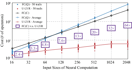
Figure 4 reports the comparison results for the core component in neural network, the neural computation layer. The x-axis represents the input size of the neural computation, and the y-axis stands for the cost, that is, the number of operators used in the corresponding design. For quantum implementation (both FC(Q)[27] in FFNN(Q)[28] and U-LYR in QuantumFlow), the value of weights will affect the gate usage, so we generate 50 sets of weights for each scale of input, and the dots on the lines in this figure represent average cost. From this figure, it clearly shows that the cost of FC(C) in MLP(C) on classical computing platforms grows exponentially along with the increase of inputs. The state-of-the-art quantum implementation FC(Q) has the similar exponentially growing trend. On the other hand, we can see that the growing trend of U-LYR is much slower. As a result, the cost reduction continuously increases along with the growth of the input size of neural computation. For the input size of 16 and 32, the average cost reductions are 2.4 and 3.3, compared with the implementations on classical computers. When the input size grows to 2,048, the cost reduction increased to 64 on average. The cost reduction trends in this figure clearly demonstrate the quantum advantage achieved by U-LYR. In the Methods section, for the neural computation with an input size of , we will show that the complexity for quantum implementation is , while it is for classical computers.
Table 2 reports the comparison results for the whole network. The neural network models for MNIST in Figure 2 are deployed to quantum circuits to get the cost. In addition, to demonstrate the scalability, we further include a new model for dataset “{0,1,3,6,9}∗”, which takes the larger sized inputs but less neurons in the first layer and having higher accuracy over “{0,1,3,6,9}”. In this table, columns , , and under three approaches report the number of gates used in the first and second layers, and in the whole network. Columns “Red.” represent the comparison with baseline .
From the table, it is clear to see that all cases implemented by QF-hNet can achieve cost reduction over MLP(C), while for datasets with more than 3 classes, FFNN(Q) needs more gates than MLP(C). A further observation made in the results is that QF-hNet can achieve higher cost reduction with the increase of input size. Specifically, for input size is 16, the reduction ranges from to . The reduction increases to for input size is 64, and it continuously increases to when the input size grows to 256. The above results are consistent with the results shown in Figure 4. It further indicates that even the second layer in QF-hNet uses the P-LYR which requires more gates for implementation, the quantum advantage can still be achieved for the whole network because the first layer using U-LYR can significantly reduce the number of gates. Above all, QuantumFlow demonstrates the quantum advantages on MNIST dataset.
QF-Circ on IBM Quantum Processor
This subsection further evaluates the efficacy of QuantumFlow on IBM Quantum Processors. We first show the importance of quantum circuit optimization in QF-Circ to minimize the number of required qbits. Based on the optimized circuit design, we then deploy a 2-input binary classifier on IBM quantum processors.
Figure 5 demonstrates the optimization of a 2-input neuron step by step. All quantum circuits in Figures 5(a)-(d) achieve the same functionality, but with a different number of required qbits. The equivalency of all designs will be demonstrated in the Supplementary Information. Design 1 in Figure 5(a) is directly derived from the design methodology presented in Methods section. To optimize the circuit using fewer qbits, we first convert it to the circuit in Figure 5(b), denoted as design 2. Since there is only one controlled-Z gate from qbit I0 to qbit E/O, we can merge these two qbits, and obtain an optimized design in Figure 5(c) with 2 qbits, denoted as design 3. The circuit can be further optimized to use 1 qbit, as shown in Figure 5(d), denoted as design 4. The function in design 4 is defined as follows:
| (1) |
where , , representing input probabilities.
To compare these designs, we deploy them onto IBM Quantum Processors, where “ibm_velencia” backend is selected by QF-Map. In the experiments, we use the results from QF-FB(C) as the golden results. Figure 5(e) reports the deviations of design 1 and design 4 against the golden results. The results clearly show that design 4 is more robust because it uses fewer qbits in the circuit. Specifically, the deviation of design 4 against golden results is always less than 5%, while reaching up to 13% for design 1. In the following experiments, design 4 is applied in QF-Circ.


Next, we are ready to introduce the case study on an end-to-end binary classification problem as shown in Figure 6. In this case study, we train the QF-pNet based on QF-FB(C). Then, the tuned parameters are applied to generate QF-Circ. Finally, QF-Map optimizes the deployment of QF-Circ to IBM quantum processor, selecting the “ibmq_essex” backend.
The classification problem is illustrated in Figure 6(a), which is a binary classification problem (two classes) with two inputs: and . For instance, if and , it indicates class 0. The QF-pNet, QF-Circ, and QF-Map are demonstrated in Figure 6(b)-(d). First, Figure 6(b) shows that QF-pNet consists of one hidden layer with one 2-input neuron and batch normalization. The output is the probability of class 0. Specifically, an input is recognized as class 0 if ; otherwise it is identified as class 1.
The quantum circuit QF-Circ of the above QF-pNet is shown in Figure 6(c). The circuit is composed of three parts, (1) neural computation, (2) batch_adj in batch normalization, and (3) indiv_adj in batch normalization. The neural computation is based on design 4 as shown in Figure 5(d). The parameter of gate in neural computation at qbit is determined by the inputs and . Specifically, , as shown in Formula 1. Then, batch normalization is implemented in two steps, where qbits and are initialized according to the trained BN parameters. During the process, holds the intermediate results after batch_adj, and holds the final results after indiv_adj. Finally, we measure the output on qbit 22 2 A Quirk-based example of inputs 0.2 and 0.6 leading to can be accessed by https://wjiang.nd.edu/quirk_0_2_0_6.html, which is accessible at 06-19-2020. The output probability of 60.3% is larger than 50%, implying the inputs belong to class 0..
After building QF-Circ, the next step is to map qbits from the designed circuit to the physic qbits on the quantum processor, and this is achieved through our QF-Map. In this experiment, QF-Map selects “ibm_essex” as backend with its physical properties shown in Figure 6(d), where error rates of each qbit and each connection are illustrated by different colors. By following the rules as defined by QF-Map (see Method section), we obtain the physically mapped QF-Circ shown in Figure 6(d). For example, the input is mapped to the physical qbit labeled as 4.
After QuantumFlow goes through all the steps from input data to the physic quantum processor, we can perform inference on the quantum computer. In this experiments, we test 100 combinations of inputs from to . First, we obtain the results using QF-FB(C) as golden results and QF-FB(Q) as quantum simulation assuming perfect qbits, which are reported in Figure 6(e) and (f), achieving 100% and 98% prediction accuracy. The results verify the correctness of the proposed QF-pNet. Second, the results obtained on quantum processors are shown in Figure 6(h), which achieves 82% accuracy in prediction. For comparison, in Figure 6(g), we also show the results obtained by using the default mapping algorithm in IBM Qiskit, whose accuracy is only 68%. This result demonstrates the value of QF-Map in further improving the physically achievable accuracy on a physical quantum processor with errors.
Discussion
In summary, we propose a holistic QuantumFlow framework to co-design the neural networks and quantum circuits. Novel quantum-aware QF-Nets are first designed. Then, an accurate and efficient inference engine, QF-FB, is proposed to enable the training of QF-Nets on classical computers. Based on QF-Nets and the training results, the QF-Map can automatically generate and optimize a corresponding quantum circuit, QF-Circ. Finally, QF-Map can further map QF-Circ to a quantum processor in terms of qbits’ error rates.
| Layers | FC(C)[38] | FC(Q)[28] | P-LYR | U-LYR | |
| Complexity | # Bits/Qbits | ||||
| # Operators | |||||
| Data Representation | Input Data | F32 | Bin | R.V. | F32 |
| Weights | Bin (F32) | Bin | Bin (R.V.) | Bin | |
| Connect Layers w/o Measurement | ✓ | - | ✓ | ||
| Summary | Flexibility | - | ✓ | ||
| Qu. Adv. | - | ✓ | |||
The neural computation layer is one key component in QuantumFlow to achieve state-of-the-art accuracy and quantum advantage. We have shown in Figure 2 that the existing quantum-aware neural network [28] that interprets inputs as the binary form will degrade the network accuracy. To address this problem, in QF-pNet, we first propose a probability-based neural computation layer, denoted as P-LYR, which interprets real number inputs as random variables following a two-point distribution. As shown in Table 3, P-LYR can represent both input and weight data using random variables, and it can directly connect layers without measurement. In summary, P-LYR provides better flexibility to perform neural computation than others; however, it suffers high complexity, i.e., for the usage of qbits and for the usage of operators (basic quantum gates).
In order to acquire quantum advantages, we further propose a unitary matrix based neural computation layer, called U-LYR. As illustrated in Table 3, U-LYR sacrifices some degree of flexibility on data representation and non-linear function but can significantly reduce the circuit complexity. Specifically, with the help of QF-Map, the number of basic operators used by U-LYR can be reduced from to , compared to FC(C) and FC(Q). Kindly note that this work does not take the cost of inputs encoding into consideration in demonstrating quantum advantage; instead, we focus on the speedup of the commonly used computation component layer, that is, the neural computation layer. The cost of encoding inputs can be reduced to by preprocessing data and storing them into quantum memory, or approximating the quantum states by using basic gate (e.g., Ry). For neural computation, we demonstrated that U-LYR can successfully achieve quantum advantage in the next section.
Batch normalization is another key technique in improving accuracy, since the backbone of the quantum-friendly neuron computation layers (P-LYR and U-LYR) is similar to that in classical computers, using both linear and non-linear functions. This can be seen from the results in Figure 2. Batch normalization can achieve better model accuracy, mainly because the data passing a nonlinear function will lead to outputs to be significantly shrunken to a small range around 0 for real number representation and for a two-point distribution representation, where is the number of inputs. Unlike straightforwardly doing normalization on classical computers, it is non-trivial to normalize a set of qbits. Innovations are made in QuantumFlow for a quantum-friendly normalization.
The philosophy of co-design is demonstrated in the design of P-LYR, U-LYR, and N-LYR. From the neural network design, we take the known operations as the backbones in P-LYR, U-LYR, and N-LYR; while from the quantum circuit design, we take full use of its ability in processing probabilistic computation and unitary matrix based computations to make P-LYR, U-LYR, and N-LYR quantum-friendly. In addition, as will be shown in the next section, the key to achieve quantum advantage for U-LYR is that QF-Map fully considers the flexibility of the neural networks (i.e., the order of inputs can be changed), while the requirement of continuously executing machine learning algorithms on the quantum computer leads to a hybrid neural network, QF-hNet, with both neural computation operations: P-LYR and U-LYR. Without the co-design, the previous works did not exploit quantum advantages in implementing neural networks on quantum computers, which reflects the importance of conducting co-design.
We have experimentally tested QuantumFlow on a 32-qbit Qiskit Aer simulator and a 5-qbit IBM quantum processor based on superconducting technology. We show that the proposed quantum oriented neural networks QF-Nets can obtain state-of-the-art accuracy on the MNIST dataset. It can even outperform the conventional model on a similar scale for the classical computer. For the experiments on IBM quantum processors, we demonstrate that, even with the high error rates of the current quantum processor, QF-Nets can be applied to classification tasks with high accuracy.
In order to accelerate the QF-FB on classical computers to support training, we make the assumptions that the perfect qbits are used. This enables us to apply theoretic formulations to accelerate the simulation process; however, it leads to some error in predicting the outputs of its corresponding deployment on a physical quantum processor with high error rates (such as the current IBM quantum processor with error rates in the range of ). However, we do not deem this as a drawback of our approach, rather this is an inherent problem of the current physical implementation of quantum processors. As the error rates get smaller in the future, it will help to narrow the gap between what QF-Nets predicts and what quantum processor delivers. With the innovations on reducing the error rate of physic qbits, QF-Nets will achieve better results.

Methods
We are going to introduce QuantumFlow in this section. Neural computation and batch normalization are two key components in a neural network, and we will present the design and implementation of these two components in QF-Nets, QF-FB, QF-Circ, and QF-Map, respectively.
QF-pNet and QF-hNet
Figure 7 demonstrates two different neural computation components in QuantumFlow: P-LYR and U-LYR. As stated in the Discussion section, P-LYR and U-LYR have their different features. Before introducing these two components, we demonstrate the common prepossessing step in Figure 7(a), which goes through the downsampling and grey level normalization to obtain a matrix with values in the range of 0 to 1. With the prepossessed data, we will discuss the details of each component in the following texts.

Neural Computation P-LYR: An m-input neural computation component is illustrated in 7(d), where input data and corresponding weights are given. Input data is a real number ranging from 0 to 1, while weight is a binary number. Neural computation in P-LYR is composed of 4 operations: i) R: this operation converts a real number of input to a two-point distributed random variable , where and , as shown in 7(b). For example, we treat the input ’s real value of as the probability of that outcomes while as the probability that outcomes . ii) C: this operation calculates as the average sum of weighted inputs, where the weighted input is the product of a converted input (say ) and its corresponding weight (i.e., ). Since is a two-point random variable, whose values are and and the weights are binary values of and , if , will lead to the swap of probabilities and in . iii) A: we consider the quadratic function as the non-linear activation function in this work, and operation outputs where is a random variable. iv) E: this operation converts the random variable to 0-1 real number by taking its expectation. It will be passed to batch normalization to be further used as the input to the next layer.

Neural Computation U-LYR: Unlike P-LYR taking advantage of the probabilistic properties of qbits to provide the maximum flexibility, U-LYR aims to minimize the gates for quantum advantage using the property of the unitary matrix. The input data are first converted to corresponding data that can be the first column of a unitary matrix, as shown in Figure 7(d). Then the linear function and activation quadratic function are conducted. U-LYR has the potential to significantly reduce the quantum gates for computation, since the inputs are the first column in a unitary matrix and can be encoded to qbits. But the state-of-the-art hypergraph based approach[27] needs basic quantum gates to encode corresponding weights to qbits, which is the same with that of classical computer needing operators (i.e., adder/multiplier). In the later section of QF-Map, we propose an algorithm to guarantee that the number of used basic quantum gates to be , achieving quantum advantages.
Multiple Layers: P-LYR and U-LYR are the fundamental components in QF-Nets, which may have multiple layers. In terms of how a network is composed using these two components, we present two kinds of neural networks: QF-pNet and QF-hNet. QF-pNet is composed of multiple layers of P-LYR. For its quantum implementation, operations on random variables can be directly operated on qbits. Therefore, R operation is only conducted in the first layer. Then, C and A operations will be repeated without measurement. Finally, at the last layer, we measure the probability for output qbits, which is corresponding to the E operation. On the other hand, QF-hNet is composed of both U-LYR and P-LYR, where the first layer applies U-LYR with the converted inputs. The output of U-LYR is directly represented by the probability form on a qbit, and it can seamlessly connect to C in P-LYR used in later layers.
Batch Normalization: Figure 8 illustrates the proposed batch normalization (N-LYR) component. It can take the output of either P-LYR or U-LYR as input. N-LYR is composed of two sub-components: batch adjustment (“batch_adj”) and individual adjustment (“indiv_adj”). Basically, batch_adj is proposed to avoid data to be continuously shrunken to a small range (as stated in Discussion section). This is achieved by normalizing the probability mean of a batch of outputs to 0.5 at the training phase, as shown in Figure 9(c)-(d). In the inference phase, the output can be computed as follows:
| (2) | ||||
After batch_adj, the outputs of all neurons are normalized around 0.5. In order to increase the variety of different neurons’ output for better classification, indiv_adj is proposed. It contains a trainable parameter and a parameter (see Figure 9(e)). It is performed in two steps: (1) we get a start point of an output according to , and then moves it back to p=0.5 to obtain parameter ; (2) we move the angle of to obtain the final output. Since different neurons have different values of , the variation of outputs can be obtained. In the inference phase, its output can be calculated as follows.
| (3) |
The determination of parameters , , and is conducted in the training phase, which will be introduced later in QF-FB.
QF-FB
QF-FB involves both forward propagation and backward propagation. In forward propagation, all weights and parameters are determined, and we can conduct neural computation and batch normalization layer by layer. For -LYp, the neural computation will compute and , where is a two-point random variable. The distributions of and are illustrated in Figure 9(a)-(b). It is straightforward to get the expectation of by using the distribution; however, for inputs, it involves terms (e.g., is one term), and leads to the time complexity to be . To reduce the time complexity, QF-FB takes advantage of independence of inputs to calculate the expectation as follows:
| (4) | ||||
where , since and there are inputs in total. The above formula derives the following algorithm with time complexity of to simulate the neural computation P-LYR.

2. Expectation of : ;
3. Sum of pair product ;
4. Expectation of : ;
5. Return ;
For -LYu, the neural computation will first convert inputs to a vector who can be the first column of a unitary matrix . By operating on qbits with initial state (i.e., ), we can encode to states. The generating of unitary matrix is equivalent to the problem of identifying the nearest orthogonal matrix given a square matrix . Here, matrix is created by using as the first column, and for all other elements. Then, we apply Singular Value Decomposition (SVD) to obtain , and we can obtain . Based on the obtained vector in , -LYu computes and , as shown in the following algorithm.
2. Calculating and extract vector from ;
3. Compute ;
4. Return ;
The forward propagation for batch normalization can be efficiently implemented based on the output of the neural computation. A code snippet is given as follows.
For the backward propagation, we need to determine weights and parameters (e.g., in N-LYR). The typically used optimization method (e.g., stochastic gradient descent [39]) is applied to determine weights. In the following, we will discuss the determination of N-LYRparameters , , .
The batch_adj sub-component involves two parameters, and . During the training phase, a batch of outputs are generated for each neuron. Details are demonstrated in Figure 9(c)-(d) with 6 outputs. In terms of the mean of outputs in a batch , there are two possible cases: (1) and (2) . For the first case, is set to 0 and can be derived from Formula 2 by setting to 0.5; similarly, for the second case, is set to 1 and . Kindly note that the training procedure will be conducted in multiple iterations of batches. As with the method for batch normalization in the conventional neural network, we employ moving average to record parameters. Let be the parameter of (e.g., ) at the iteration, and be the value obtained in the current iteration. For , it can be calculated as , where is the momentum which is set to by default in the experiments.
In forward propagation, the sub-module indiv_adj is almost the same with batch_adj for ; however, the determination of its parameter is slightly different from for batch_adj. As shown in Figure 9(e), the initial probability of after batch_adj is . The basic idea of indiv_adj is to move by an angle, . It will be conducted in three steps: (1) we move start point at to point with the probability of , where is the batch size and is a trainable variable; (2) we obtain by moving point to ; (3) we finally move solution at by the angle of to obtain the final result. By replacing by in batch_adj when , we can calculate . For each batch, we calculate the mean of , and we also employ the moving average to record .
QF-Circ
We now discuss the corresponding circuit design for components in QF-Nets, including P-LYR, U-LYR, and N-LYR. Figures 10(a)-(b) demonstrate the circuit design for P-LYR (see Figure 7(c)) and U-LYR (see Figure 7(e)), respectively; Figures 10(c)-(f) demonstrate the N-LYR in Figure 8.
Implementing P-LYR on quantum circuit: For an -input neural computation, the quantum circuit for P-LYR is composed of input qbits (I), and encoding qbits (E), and 1 output qbit (O).
In accordance with the operations in P-LYR, the circuit is composed of four parts. In the first part, the circuit is initialized to perform R operation. For qbits , we apply Ry gates with parameter to initialize the input qbit in terms of the input real value , such that the state of is changed from to . For encoding qbits and output qbit , they are initialized as . The second part completes the average sum function, i.e., C operation. It further includes three steps: (1) dot product of inputs and weights on qibits , (2) make encoding qbits into superposition, (3) encode probabilities in qbits to states in qbits . The third part implements the quadratic activation function, that is the A operation. It applies the control gate to extract the amplitudes in states to qbit . As we know that the probability is the square of the amplitude, the quadratic activation function can be naturally implemented. Finally, E operations corresponds to the fourth part that measures qbit to obtain the output real number , where the state of is . A detailed demonstration of the equivalency between QF-Circ and P-LYR can be found in the Supplementary Information.
Kindly note that for a multi-layer network composed of P-LYR, namely QF-pNet, there is no need to have a measurement at interfaces, because the converting operation initializes a qbit to the state exactly the same with . In addition, the batch normalization can also take as input.
Implementing U-LYR on quantum circuit: For an -input neural computation, the quantum circuit for U-LYR contains encoding qbits and 1 output qbit .
According to U-LYR, the circuit in turn performs U, , operations, and finally obtains the result by a measurement. In the first operation, unlike the circuit for P-LYR using gate to initialize circuits using qbits; for U-LYR, we using the matrix to initialize circuits on qbits . Recalling that the first column of is vector , after this step, elements in vector will be encoded to states represented by qbits . The second operation is to perform the dot product between all states in qbits and weights , which is implemented by control Z gates and will be introduced in QF-Map. Finally, like the circuit for P-LYR, the quadratic activation and measurement are implemented. Kindly note that, in addition to quadratic activation, we can also implement higher orders of non-linearity by duplicating the circuit to perform U, , and to achieve multiple outputs. Then, we can use control NOT gate on the outputs to achieve higher orders of non-linearity. For example, using a Toffoli gate on two outputs can realize . Let the non-linear function be and the cost complexity of U-LYR using quadratic activation be , then the cost complexity of U-LYR using as the non-linear function will be .
For neural networks with given inputs, we can preprocess the U operation and store the states in quantum memory [40]. Thus, the key for quantum advantage is to exponentially reduce the number of gates used in neural computation, compared with the number of basic operators used in classical computing. We will present an algorithm in QF-Map for U-LYR to achieve this goal.
Implementing N-LYR on quantum circuit: Now, we discuss the implementation of N-LYR in quantum circuits. In these circuits, three qbits are involved: (1) qbit for input, which can be the output of qbit in circuit without measurement, or initialized using a Ry gate according to the measurement of qbit in circuit; (2) qbit conveys the parameter, which is obtained via training procedure, see details in QF-FB; (3) output qbits , which can be directly used for the next layer or be measured to convert to a real number.
Figures 10(b)-(c) show the circuit design for two cases in batch_adj. Since parameters in batch_adj are determined in the inference phase, if , we will adopt the circuit in Figure 10(b), otherwise, we adopt that in Figure 10(c). Then, Figure 10(d) shows the circuit for indiv_adj. We can see that circuits in Figures 10(c) and (d) are the same except the initialization of parameters, and . For circuit optimization, we can merge the above two circuits into one by changing the input parameters to , as shown in Figure 10(e). In this circuit, , while for applying circuits in Figures 10(c) and (d), we will have . To guarantee the consistent function, we can derive that .
QF-Map
QF-Map is an automatic tool to map QF-Nets to the quantum processor through two steps: network-to-circuit mapping, which maps QF-Nets to QF-Circ; and virtual-to-physic mapping, which maps QF-Circ to physic qbits.
Mapping QF-Nets to QF-Circ: The first step of QF-Map is to map three kinds of layers (i.e., P-LYR, U-LYR, and N-LYR) to QF-Circ. The mappings of P-LYR and N-LYR are straightforward. Specifically, for P-LYR in Figure 10(a), the circuit for weight is determined using the following rule: for a qbit , an gate is placed if and only if . Let the probability , after the gate, the probability becomes . Since the values of random variable are and , such an operation computes . For N-LYR, let be the output qbit of the first layer. It can be directly connected to the qbit in Figure 10(c)-(f), according to the type of batch normalization, which is determined by the training phase.
The mapping of U-LYR to quantum circuits is the key to achieve quantum advantages. In the following texts, we will first formulate the problem, and then introduce the proposed algorithm to guarantee the cost for a neural computation with inputs to be .
Before formally introducing the problem, we first give some fundamental definitions that will be used. We first define the quantum state and the relationship between states as follows. Let the computational basis be composed of qbits, as in Figure 10(b). Define to be the state, where is a binary number and . For two states and , we define if , we have . We define to be the sign of .

Next, we define the gates to flip the sign of states. The controlled operation among qbits (e.g., ) is a quantum gate to flip the sign of states [25, 27]. Define to be a gate to flip the state only. It can be implemented as follows: if , the control signal of the qbit is enabled by , otherwise if , it is enabled by . Define to be a controlled Z gate to flip all states if . It can be implemented as follows: if , there is a control signal of the qbit, enabled by , otherwise, it is not a control qbit. Specifically, if there is only for all , we put a gate on the qbit. Figure 11 illustrates , and . We define cost function to be the number of basic gates (e.g., Pauli-X, Toffoli) used in a control Z gate.
Now, we formally define the weight mapping problem as follows: Given (1) a vector with binary weights (i.e., -1 or +1) and (2) a computational basis of qbits that include states and , is , the problem is to determine a set of gates in either or to be applied, such that the circuit cost is minimized, while the sign of each state is the same with the corresponding weight; i.e., , and , where is the sign of state under the computing conducted by a sequence of quantum gates in .
A straightforward way to satisfy the sign flip requirement without considering cost is to apply for all states whose corresponding weights are . A better solution for cost minimization is to use hypergraph states[27], which starts from the states with less , and apply to reduce the cost. However, as shown in the previous work, both methods have the cost complexity of , which is the same as classical computers and no quantum advantage can be achieved.
Toward the quantum advantage, we made the following important observation: the order of weights can be adjusted, since matrix obtained by switching two rows in the unitary matrix will still be a unitary matrix. Based on this property, we can simplify the weight mapping problem to determine a set of gates, such that the cost is minimized while the number of states with sign flip is the same as the number of in weight . On top of this, we propose an algorithm to guarantee the cost complexity to be . Compared to needed for classical computers, we can achieve quantum advantages. To demonstrate how to guarantee the cost complexity to be , we first have the following theorem.
Theorem 1.
For an integer number where and , the number can be expressed by a sequence of addition () or subtraction () of a subset of ; when the terms of are sorted in a descending order, the sign of the expression (addition and subtraction) are alternative with the leading sign being addition ().
Proof.
The above theorem can be proved by induction. First, for , the possible values of are , the set . The theorem is obviously true. Second, for , the possible values of are , and the set . In this case, only needs to involve 2 numbers from using the expression ; other numbers can be directly expressed by themselves. So, the theorem is true.
Third, assuming the theorem is true for , we can prove that for the theorem is true for the following three cases. Case 1: For , since the theorem is true for , based on the assumption, all numbers less than can be expressed by using set and thus we can also express them by using set because ; Case 2: For , itself is in set ; Case 3: For , we can express , where . Since the theorem is true for , we can express by using set ; hence, can be expressed using set .
Above all, the theorem is correct. ∎
We propose to only use gate in a set for any required number of sign flips on states; for instance, if , the gate set is and . This can be demonstrated using the above theorem and properties of the problem: (1) the problem has symmetric property due to the quadratic activation function. Therefore, the weight mapping problem can be reduced to find a set of gates leading to the number of no larger than ; i.e., . (2) for , it will flip the sign of states; since , the numbers of the flipped sign by these gates belong to a set ; These two properties make the problem in accordance with that in Theorem 1. The weight mapping problem is also consistent with three rules in the theorem. (1) A gate can be selected or not, indicating the finally determined gate set is the subset of ; (2) all states at the beginning have the positive sign, and therefore, the first gate will increase sign flips, indicating the leading sign is addition (); (3) , ; it indicates that among the states whose signs are flipped by , there are states signs are flipped back; this is in accordance to alternatively use and in the expression in Theorem 1. Followed by the proof procedure, we devise the following recursive algorithm to decide which gates to be employed.
if {
recursive(,,); // Case 1 in the third step
}
else if {
; // Case 2 in the third step
return;
}else{
;
recursive(,,); // Case 3 in the third step
}
}
// Entry of weight mapping algorithm
set main(,){
Initialize empty set ;
recursive(,,);
return
}
In the above algorithm, the worst case for the cost is that we apply all gates in . Let the state has states, if the can be implemented using basic gates, including Toffoli gates for controlling, 1 control Z gate, and Toffoli gates for resetting; otherwise, it uses 1 basic gates. Based on these understandings, we can calculate the cost complexity in the worst case, which is . Therefore, the cost complexity of linear function computation is . The quadratic activation function is implemented by a gate, whose cost is . Thus, the cost complexity for neural computation U-LYR is .
Finally, to make the functional correctness, in generating the inputs unitary matrix, we swap rows in it in terms of the weights, and store the generated results in quantum memory.
Mapping QF-Circ to physic qbits: After QF-Circ is generated, the second step is to map QF-Circ to quantum processors, called virtual-to-physic mapping. In this paper, we deploy QF-Circ to various IBM quantum processors. Virtual-to-physic mapping in QF-Map has two tasks: (1) select a suitable quantum processor backend, and (2) map qbits in QF-Nets to physic qbits in the selected backend. For the first task, QF-Map will i) check the number of qbits needed; ii) find the backend with the smallest number of qbit to accommodate QF-Circ; iii) for the backends with the same number of qbits, QF-Map will select a backend for the minimum average error rate. The second task in QF-Map is to map qbits in QF-Nets to physic qbits. The mapping follows two rules: (1) the qbit in QF-Nets with more gates is mapped to the physic qbit with a lower error rate; and (2) qbits in QF-Nets with connections are mapped to the physic qbits with the smallest distance.
Data availability
The authors declare that all data supporting the findings of this study are available within the article and its Supplementary Information files. Source data can be accessed via https://wjiang.nd.edu/categories/qf/.
Code availability
All relevant codes will be open in github upon the acceptance of the manuscript or be available from the corresponding authors upon reasonable request.
References
- [1] Shor, P. W. Polynomial-time algorithms for prime factorization and discrete logarithms on a quantum computer. SIAM review 41, 303–332 (1999).
- [2] Arute, F. et al. Quantum supremacy using a programmable superconducting processor. Nature 574, 505–510 (2019).
- [3] LeCun, Y., Bengio, Y. & Hinton, G. Deep learning. nature 521, 436–444 (2015).
- [4] Goodfellow, I., Bengio, Y. & Courville, A. Deep learning (MIT press, 2016).
- [5] Szegedy, C. et al. Going deeper with convolutions. In Proceedings of the IEEE conference on computer vision and pattern recognition, 1–9 (2015).
- [6] Krizhevsky, A., Sutskever, I. & Hinton, G. E. Imagenet classification with deep convolutional neural networks. In Advances in neural information processing systems, 1097–1105 (2012).
- [7] He, K., Zhang, X., Ren, S. & Sun, J. Deep residual learning for image recognition. In Proceedings of the IEEE conference on computer vision and pattern recognition, 770–778 (2016).
- [8] Simonyan, K. & Zisserman, A. Very deep convolutional networks for large-scale image recognition. arXiv preprint arXiv:1409.1556 (2014).
- [9] Szegedy, C., Vanhoucke, V., Ioffe, S., Shlens, J. & Wojna, Z. Rethinking the inception architecture for computer vision. In Proceedings of the IEEE conference on computer vision and pattern recognition, 2818–2826 (2016).
- [10] Lin, T.-Y. et al. Feature pyramid networks for object detection. In Proceedings of the IEEE conference on computer vision and pattern recognition, 2117–2125 (2017).
- [11] Ren, S., He, K., Girshick, R. & Sun, J. Faster r-cnn: Towards real-time object detection with region proposal networks. In Advances in neural information processing systems, 91–99 (2015).
- [12] He, K., Gkioxari, G., Dollár, P. & Girshick, R. Mask r-cnn. In Proceedings of the IEEE international conference on computer vision, 2961–2969 (2017).
- [13] Ronneberger, O., Fischer, P. & Brox, T. U-net: Convolutional networks for biomedical image segmentation. In International Conference on Medical image computing and computer-assisted intervention, 234–241 (Springer, 2015).
- [14] Young, T., Hazarika, D., Poria, S. & Cambria, E. Recent trends in deep learning based natural language processing. ieee Computational intelligenCe magazine 13, 55–75 (2018).
- [15] Sak, H., Senior, A. & Beaufays, F. Long short-term memory recurrent neural network architectures for large scale acoustic modeling. In Fifteenth Annual Conference of the International Speech Communication Association (2014).
- [16] Vaswani, A. et al. Attention is all you need. In Advances in neural information processing systems, 5998–6008 (2017).
- [17] Bernard, O. et al. Deep learning techniques for automatic MRI cardiac multi-structures segmentation and diagnosis: is the problem solved? IEEE transactions on medical imaging 37, 2514–2525 (2018).
- [18] Bonaldi, A. & Braun, R. Square kilometre array science data challenge 1. arXiv preprint arXiv:1811.10454 (2018).
- [19] Lukic, V., de Gasperin, F. & Brüggen, M. ConvoSource: Radio-Astronomical Source-Finding with Convolutional Neural Networks. Galaxies 8, 3 (2020).
- [20] Xu, X. et al. Scaling for edge inference of deep neural networks. Nature Electronics 1, 216–222 (2018).
- [21] Steffen, M., DiVincenzo, D. P., Chow, J. M., Theis, T. N. & Ketchen, M. B. Quantum computing: An ibm perspective. IBM Journal of Research and Development 55, 13–1 (2011).
- [22] Schuld, M., Sinayskiy, I. & Petruccione, F. An introduction to quantum machine learning. Contemporary Physics 56, 172–185 (2015).
- [23] Bertels, K. et al. Quantum computer architecture: Towards full-stack quantum accelerators. arXiv preprint arXiv:1903.09575 (2019).
- [24] Cai, X.-D. et al. Entanglement-based machine learning on a quantum computer. Physical review letters 114, 110504 (2015).
- [25] Nielsen, M. A. & Chuang, I. Quantum computation and quantum information (2002).
- [26] Broughton, M. et al. Tensorflow quantum: A software framework for quantum machine learning. arXiv preprint arXiv:2003.02989 (2020).
- [27] Tacchino, F., Macchiavello, C., Gerace, D. & Bajoni, D. An artificial neuron implemented on an actual quantum processor. npj Quantum Information 5, 1–8 (2019).
- [28] Tacchino, F. et al. Quantum implementation of an artificial feed-forward neural network. arXiv preprint arXiv:1912.12486 (2019).
- [29] Rebentrost, P., Bromley, T. R., Weedbrook, C. & Lloyd, S. Quantum hopfield neural network. Physical Review A 98, 042308 (2018).
- [30] Schuld, M., Sinayskiy, I. & Petruccione, F. The quest for a quantum neural network. Quantum Information Processing 13, 2567–2586 (2014).
- [31] McCulloch, W. S. & Pitts, W. A logical calculus of the ideas immanent in nervous activity. The bulletin of mathematical biophysics 5, 115–133 (1943).
- [32] Havlíček, V. et al. Supervised learning with quantum-enhanced feature spaces. Nature 567, 209–212 (2019).
- [33] Shi, Y.-Y., Duan, L.-M. & Vidal, G. Classical simulation of quantum many-body systems with a tree tensor network. Physical review a 74, 022320 (2006).
- [34] Grant, E. et al. Hierarchical quantum classifiers. npj Quantum Information 4, 1–8 (2018).
- [35] Courbariaux, M., Bengio, Y. & David, J.-P. Binaryconnect: Training deep neural networks with binary weights during propagations. In Advances in neural information processing systems, 3123–3131 (2015).
- [36] LeCun, Y., Bottou, L., Bengio, Y. & Haffner, P. Gradient-based learning applied to document recognition. Proceedings of the IEEE 86, 2278–2324 (1998).
- [37] Google. TensorFlow Quantum. https://www.tensorflow.org/quantum/tutorials/mnist (2020). Accessed: 2020-08-18.
- [38] Rosenblatt, F. The perceptron, a perceiving and recognizing automaton Project Para (Cornell Aeronautical Laboratory, 1957).
- [39] Bottou, L. Large-scale machine learning with stochastic gradient descent. In Proceedings of COMPSTAT’2010, 177–186 (Springer, 2010).
- [40] Lvovsky, A. I., Sanders, B. C. & Tittel, W. Optical quantum memory. Nature photonics 3, 706–714 (2009).
Acknowledgements
This work is partially supported by IBM and University of Notre Dame (IBM-ND) Quantum program.
Author contributions statement
W.J. conceived the idea and performed quantum evaluations; J.X. and Y.S. supervised the work and improved the idea and experiment design. All authors contributed to manuscript writing and discussions about the results.