Paths of rectangles inscribed in lines over fieldsThanks: August 11, 2026
Abstract.
We study rectangles inscribed in lines in the plane by parametrizing these rectangles in two ways, one involving slope and the other aspect ratio. This produces two paths, one that finds rectangles with specified slope and the other rectangles with specified aspect ratio. We describe the geometry of these paths and its dependence on the choice of four lines. Our methods are algebraic and work over an arbitrary field.
1991 Mathematics Subject Classification
Primary 51N10; Secondary 11E101. Introduction
Given four lines in the plane that are not all parallel, there is a rectangle whose vertices lie on these lines; i.e., the rectangle is inscribed on the lines. There are always more inscribed rectangles nearby and all of these rectangles appear as part of a path of inscribed rectangles through the configuration of lines. The purpose of this article is to account for all these rectangles by describing the paths they take through the configuration, and to do so by locating them by their slope and aspect ratio. Our methods are algebro-geometric, elementary and work over an arbitrary field. While it is possible to prove some of the results of the paper computationally, the equations in raw form are often unwieldy and opaque, so we have sought to give algebraic insight into how the geometry of the solution depends on the initial four lines.
The present article continues our study [4] but is mostly independent of this previous work, where the problem of finding inscribed rectangles was recast as that of finding the intersection of hyperbolically rotated cones in . Schwartz [6] has also recently treated rectangles inscribed in lines in the case in which none of the lines involved are parallel or perpendicular to each other. The indirect motivation for both Schwartz’s work and ours is the so-called square peg problem—a problem that remains open in full generality—of finding a square inscribed in every simple closed curve in the plane. By a theorem of Vaughn [3, p. 71], every simple closed curve in the plane has a rectangle inscribed it. In particular, every polygon has a rectangle inscribed in it, and in fact has a square inscribed in it [1]. While Vaughn’s proof guarantees that an inscribed rectangle must exist, it does not give a means for finding the rectangle, even when the curve in question is a polygon. To find a rectangle inscribed in a polygon amounts to finding a rectangle inscribed in four possibly non-distnct lines, which brings us to the current problem of finding all rectangles inscribed in four lines, as well as locating these rectangles by their slopes and aspect ratios.
Schwartz’s approach is a mix of computational and topological methods based on the geometry of the real plane, and so while some of his methods don’t extend to arbitrary fields (or because they don’t extend to fields), the difference of his methods when contrasted with ours shows some of the richness of the problem. The two approaches often differ in methods (algebro-geometric properties of fields vs. topological and analytic properties of the real plane) and in the directions these results are carried in search of finer-grained consequences. We explain in the course of the paper the points of overlap with Schwartz’s article, but briefly, Schwartz works over the field of real numbers and under the assumption that none of the lines are parallel or perpendicular. Avoiding parallel lines is needed to reduce the study of inscribed rectangles to the study of their centers only, and hence to points in . Without this restriction, two inscribed rectangles may share the same center and so information can be lost when considering only rectangle centers.
We allow parallel and perpendicular lines throughout, and to do so we view inscribed rectangles as points in a four-dimensional projective space. We find two paths of inscribed rectangles in this space, one parameterized by rectangle slope and the other by aspect ratio. Our point of view permits paths of rectangles to pass through rectangles inscribed at infinity for the four lines. We study these rectangles in some detail because they help shed light on the rectangles inscribed in the four lines in affine space. In the case in which the four lines form a non-degenerate configuration, a case explained shortly and which is described in Section 8, Schwartz has versions of these parameterizations in affine space and in his setting of no parallel or perpendicular lines. See Section 6 for a discussion of this.
Some calculations involving the data of the four lines are necessary, but we have tried to frontload these early in the paper so as to give streamlined and more conceptual proofs later. One of the main goals of the paper is to pinpoint the essential quantities needed for finding the paths of inscribed rectangles. These quantities turn out to be the slopes of the diagonals of the configuration.
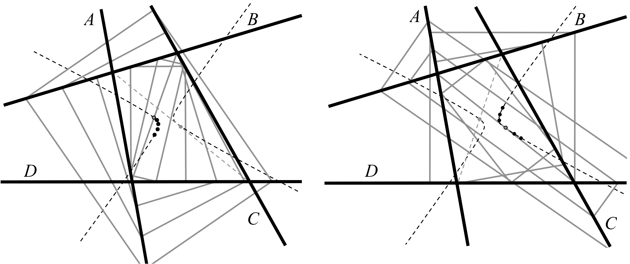

For the purpose of giving intuition, we briefly describe the behavior of the rectangles inscribed in four lines . Figure 1 shows two sets of rectangles inscribed on four lines in . These examples suggest a path of rectangles, and it is with the description of this path that the paper is concerned. The rectangles whose vertices are inscribed in sequence in the lines can be viewed as points in the set . For additional flexibility, we consider not just but all scaled copies of and their rectangles. The union of these sets is a five-dimensional vector space and so we may consider its projective space . For our purposes, turns out to be the place to work. Thus we shift focus to projective space and work out the geometry of the inscribed rectangles there.
We show in Section 3 that the points in that represent the inscribed rectangles comprise a plane curve of degree . This curve, as we show in Sections 5 and 6, is the union of two paths: a slope path given by a regular map that sends a ratio represented as a point on the projective line to a rectangle having this slope, and an aspect path given by a regular map that sends a ratio to a rectangle having this aspect ratio. These paths pick up additional rectangles, those that are inscribed at infinity for the configuration, and these rectangles are the subject of Section 4. In any case, the slope and aspect paths solve the problem of finding the rectangles of specified slope and aspect ratio. In Sections 5 and 6 we give succinct versions of the defining polynomials for these paths in order to exhibit some of the internal symmetry of the algebra of the paths. The formulations of these polynomials belong to our main results. The two paths share a number of formal features that suggest more could be learned about the relationship between them.
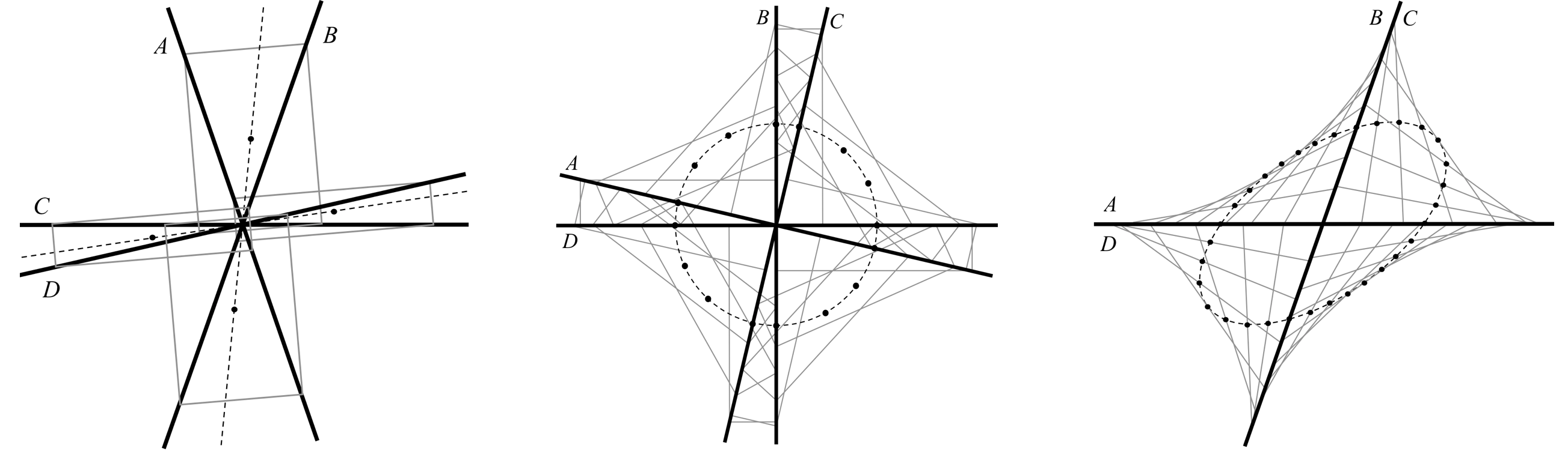
In Sections 7 and 8 we show that the slope and aspect paths either (a) have exactly the same image in , and thus find the same rectangles, or (b) they are distinct lines of rectangles. Case (b) occurs precisely if the diagonals of the configuration are orthogonal (Theorem 7.1). In case (a), the affine piece of the curve of rectangles in is a non-degenerate conic (Theorem 7.1), which if is a hyperbola (Theorem 3.6). Otherwise, in case (b), each path is a line, so the two lines form a degenerate conic. (It can happen that one of these lines is the line at infinity.) Case (b) is illustrated by the examples in Figure 2. In Section 9 we go further with the degenerate case and interpret the paths of the centers of the rectangles in these two lines geometrically.
A final word on generality: Even though our main motivation is the case in which is the field of real numbers, we work with an arbitrary field for two reasons. First, doing so comes at no extra expense since our arguments are algebro-geometric and need no modification to be cast in the general setting of fields. So while we have no specific application in mind for, say, rectangles over finite fields, our approach does apply to such rectangles without any additional effort so it seems worthwhile to note this, as also it emphasizes the purely algebraic nature of our arguments. Our approach is therefore similar in spirit to the texts [2] and [5] of Kaplansky and Samuel. Second, working over a field makes it possible to find rectangles whose vertices are restricted to a subfield of the real numbers. For example, by applying the results of the paper to the field of rational numbers, we find inscribed rectangles in the real plane whose vertices have rational coordinates.
We used MapleTM to assist with calculations and examples.
2. Complete quadrilaterals in the projective plane
Throughout the paper denotes a field. In only a few instances the choice of field matters, and it is only in these cases we put additional hypotheses on . The reductions made in the following standing assumptions, which will be in force for the rest of the article, simplify the presentation and as explained below essentially result in no loss of generality when working with four not necessarily distinct lines that (a) are not all parallel, (b) do not all go through the same point, and (c) are not vertical. The condition (c) is used to simplify equations and in almost all situations, reflection about a line through the origin allows us to reduce to this case. For example, this is possible if the field has characteristic other than and at least 9 elements. This follows from [2, Theorem 14, p. 18].
Standing assumptions. Throughout this article we work with two pairs of lines and such that ; and are not parallel; and there are constants such that the equations defining the lines are
To help with later notation, we also let and so that each line is defined by an equation of the form . The following quantities, which are interpreted in Lemma 2.4, will play a fundamental role in our calculations. We write for , for , etc..
In seeking rectangles inscribed in four lines , , , satisfying (a), (b) and (c) above, we can reduce to the standing assumptions as follows. First, we can relabel lines within the pairs and to guarantee that and are not parallel. A translation then guarantees that and meet at the origin. If goes through the origin, we can switch the labels of and with those of and so as to arrange that does not pass through the origin. Scaling allows us to assume the -intercept of is . Note also that can be equal to or , and so the standing assumptions cover the case of rectangles inscribed in lines.
We work often in projective space. For this, we use standard notation for homogeneous coordinates: If , with not all the equal to , then
Projective -space, the collection of all such points , is denoted . The points at infinity for are the points of the form , where the are in and not all zero. With this in mind, in the next definition we view the configuration of the four lines as defining axes on which lie the vertices of the inscribed rectangles. We allow for scaled copies of these axes, something that will be important for defining rectangles in four-dimensional projective space.
Definition 2.1.
For each line and , let be the line in whose equation is . Let
Define a subspace of by
Alternatively, can be viewed as the the projective space of the five-dimensional subspace of . The points at infinity for are the points in with .
The special case (i.e., where ) is a configuration of the four lines through the origin. These is the configuration viewed from infinity, and it plays an important role in analyzing rectangles at infinity for .
In the next section we will interpret parallelograms and rectangles in the plane as points in , a flexibility that allows us to define rectangles at infinity also. To do so, it is helpful to view the lines as lines in the projective plane that form a complete quadrilateral that consists of four lines and six points of intersection, where some of these six points are possibly at infinity. These six points give rise to three diagonals. (Because we work over a field, the notion of a segment of a line may not have meaning, so we view our diagonals as lines rather than segments.)

Definition 2.2.
We define the diagonals and for the configuration as follows.
- (1)
If , then is the line in through the origin (the intersection of and ) and the intersection of and , which is possibly at infinity. Otherwise, if , then is the line through the origin that is orthogonal to , i.e., the line defined by .
- (2)
If , then is the line in through the intersection of and and that of and . Otherwise, if , then is the line through the intersection of and that is orthogonal to .
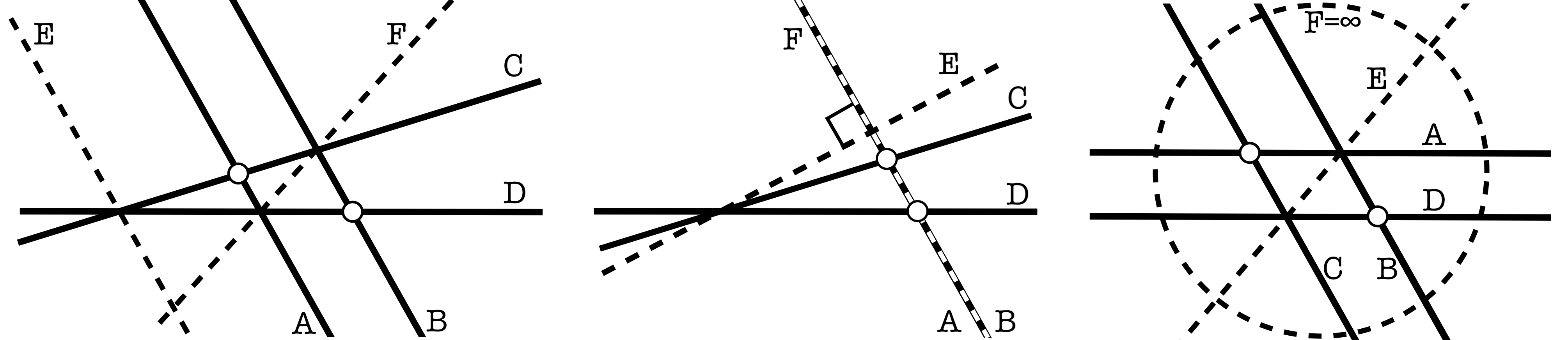
The third diagonal for the configuration can be defined similarly but only a special case of it will be needed, and not until Section 9, so we define it there. Figure 3 exhibits some complete quadrilaterals and their diagonals in the case in which no two lines are parallel. The case in which some of the lines are parallel is clarified by the following remark and Figure 4.
Remark 2.3.
- (1)
If and , then is the line through the intersection of and that is parallel to and ; see the first configuration in Figure 4. If , then coincides with and as in the second configuration, and is an altitude for the triangle that is formed from the four lines in .
- (2)
If and , then is the line at infinity; see the third configuration in Figure 4. Otherwise, if and intersect in a single point and and are parallel, then is the line parallel to and through this point. Similarly, if and intersect in a single point and and are parallel and distinct, then is the line through the point that is parallel to and .
We end this section with a technical lemma that explains the significance of the constants from the standing assumptions. The purpose of the lemma and the formulation of the constants is to shift what would be tedious case-by-case calculations throughout the paper to a few such calculations here in this proof. The lemma refers to the slope of a line, which will have the usual meaning, but which we often interpret as a point on the projective line so as to have some flexibility with infinite slope. Specifically, we view the slope of a line through two distinct points and in as the point , and we write this equivalence class as , where possibly . We continue also to represent slopes such as etc., as an element of but sometimes interpret as the point .
Lemma 2.4.
if and only if . Otherwise, if , the slope of is . Similarly, or is the line at infinity if and only if . Otherwise, the slope of is .
Proof.
If , then and , so and hence . The converse is clear. Now suppose that . If , then by Remark 2.3, . Since , this implies that . Thus so that has slope . Otherwise, if is not parallel to , then and intersect in the point
Since and intersect at the origin, the slope of is .
We show next that iff or and . Suppose that . Then yields
Since is not parallel to , it must be that . Thus . If , then and and ; otherwise, if , then . This proves that if , then or is the line at infinity. The converse is straightforward.
It remains to prove the last assertion. Suppose that , and is not parallel to . Then and . Also, . Therefore,
Thus the slope of is . A similar argument shows that if and is not parallel to , then the slope of is again .
Finally, suppose that is not parallel to and is not parallel to . The two points
are the points of intersection of and and and , respectively. The slope of the line through these two points is
which proves the lemma. ∎
3. The curve of inscribed rectangles
We define parallelograms and rectangles inscribed in the lines as points in .
Definition 3.1.
Let . A parallelogram in is a point such that and . The points are the vertices of the parallelogram. A parallelogram in is a point such that is a parallelogram in . The parallelogram is at infinity if . We allow the possibility that two or more of the vertices are the same point, and in this case, we say that the parallelogram is degenerate.
Thus the parallelograms inscribed in sequence11 1 A parallelogram in has vertices inscribed in sequence in the lines . If we wish to find parallelograms or rectangles whose vertices fall in a different sequence, we would define the Cartesian product using the lines in a different sequence. As discussed in [4, Section 4], finding all rectangles inscribed on four lines requires finding all the rectangles inscribed in 21 configurations involving these four lines. (In some of these configurations, two pairs of lines share a line; these configurations are needed to find the rectangles having two vertices on the same line.) In any case, the important point here is: Finding rectangles inscribed in lines reduces to finding the rectangles in . in the lines are the parallelograms in . Those inscribed in scaled copies of are the parallelograms in . A parallelogram in is an equivalence class of the scaled copies of a parallelogram in or , the latter being the parallelograms at infinity.
Rectangles are parallelograms whose vertices are subject to an additional condition:
Definition 3.2.
Let . A rectangle is a parallelogram such that A rectangle in is a parallelogram such that is a rectangle in . The rectangle is at infinity if . See Figure 5 for examples of rectangles at infinity.
If is the field of real numbers, then the equation in Definition 3.2 implies that the line passing through the parallelogram’s vertices on lines and is perpendicular to the line passing through the vertices on and . Interpreting this condition as an orthogonality condition for fields that are not formally real can be problematic: If is the field of complex numbers, then the same line can be “orthogonal” to itself under this definition (e.g., the line has this property). Thus for fields such as the field of complex numbers, what we are calling rectangles may not match with other natural notions of rectangles defined using inner products more typical for the choice of such a field.22 2 For simplicity’s sake, in this article we work only in the case in which the inner product is the dot product. In a future paper, when we need to work over an inner product space, we will view the inner product space as a linear transformation of a vector space equipped with the dot product and in doing so apply the results of the current paper. But our primary interest is in formally real fields, including itself, and in these cases, our algebraic rectangles reflect an obvious choice of orthogonality relation.
Theorem 3.3.
The set of parallelograms in is a plane, and the set of rectangles is a curve of degree in this plane. The line at infinity for this plane is the set of parallelograms at infinity, while the points at infinity for the curve of rectangles in the plane are the rectangles at infinity.
Proof.
To prove that the set of parallelograms in is a plane, it suffices to show that a point is a parallelogram if and only if
| (1) |
Suppose that is a parallelogram. Using the fact that the vertices of lie on the lines , we have
and
Rewriting,
Now since the lines and are not parallel, so
Thus is as claimed. Since , we have also that .
Conversely, if satisfy the equations in , then the above matrix calculations show
so defines a parallelogram in .
Now let be indeterminates for . Define a polynomial by
Applying the relevant definitions and using , the rectangles in are the parallelograms in of the form where are the zeroes of the polynomial
It follows that the set of rectangles in is a curve of degree in the plane of parallelograms in . The points at infinity for this plane are the points in of the form , where is a parallelogram in . Thus the points at infinity in the plane of parallelograms are the parallelograms at infinity, and similarly the rectangles at infinity are the points at infinity for the curve of rectangles. ∎
As we see in the next lemma, outside of one special case there are at most two rectangles at infinity. We discuss rectangles at infinity in more detail in the next section. For now, we need them in the proof of Theorem 3.6 in order to better identify the nature of the curve of rectangles in . In order to formulate Lemma 3.5, we give names in Definition 3.4 to two types of configuration of the lines that appear in the lemma and recur often in this article as exceptional cases. We say that a line with slope is orthogonal to a line with slope (written ) if . We adopt the convention that the line at infinity for is orthogonal to every line in .
Definition 3.4.
- (1)
has twin pairs if and or and .
- (2)
has dual pairs if and either or .
If has dual pairs, then , and so the condition of dual pairs cannot occur if is formally real. In the case , an elliptic cone with apex in the -plane can be associated to each of the pairs and as in [4]. The configuration has twin pairs if and only if these cones are identical, unrotated copies of each other, the only difference being that their apexes are in different locations. See Proposition 4.3 of [4] and its proof.
Lemma 3.5.
Every parallelogram at infinity in is a rectangle at infinity if and only if has twin pairs or dual pairs. If does not have twin pairs or dual pairs, then there are at most two rectangles at infinity in , and if , there are exactly two.
Proof.
With polynomials and as in the proof of Theorem 3.3, the rectangles at infinity are the parallelograms in for which . Every parallelogram at infinity in is a rectangle at infinity if and only if is identically . To prove the first assertion of the lemma, we show that if and only if has twin pairs or dual pairs.
Expanding , a calculation shows
where Thus if and only if
- (i)
or ;
- (ii)
or ; and
- (iii)
.
If has twin pairs or dual pairs, then (i), (ii) and (iii) clearly hold. Conversely, if both pairs and are orthogonal, then has twin pairs, so suppose that at least one of the pairs is not orthogonal, say and are not orthogonal. By (i), . If , then has twin pairs, so suppose that . By (ii), , and by (iii), . Thus has dual pairs. On the other hand, if and are not orthogonal, then . If , then has twin pairs. Otherwise, if , then by (i), , and so by (iii), , so that has dual pairs. This proves the first assertion of the lemma.
Now suppose that does not have twin pairs or dual pairs. Then is not identically zero, so this polynomial is homogeneous of degree . Therefore, there are most two zeroes of in . Suppose that . We show that are exactly two zeroes in for this polynomial. A calculation shows the discriminant of is
We claim that if , then has twin pairs. Suppose . Then , and since all four lines are not parallel, at least one of these slopes is nonzero, say . Thus , and so from we obtain This along with and implies that has twin pairs, a contradiction. Similarly, if , then another calculation shows that , and again has twin pairs. Symmetric arguments involving and instead of and also yield that has twin pairs. Therefore, if does not have twin pairs, then , and has two zeroes in . Consequently, there are two rectangles at infinity for . ∎
If , then the set of rectangles in is a conic by Theorem 3.3. The nature of this conic when restricted to is clarified by the next theorem.
Theorem 3.6.
If , then the set of rectangles in is a line if and only if has twin pairs. Otherwise, the set of rectangles in is a planar hyperbola.
Proof.
By Theorem 3.3, the set of rectangles in is a conic in the plane of parallelograms in . Suppose first that has twin pairs. By Lemma 3.5, the line at infinity for the plane of parallelograms in consists of rectangles at infinity. Since has twin pairs, we have either that and or and . In either case, if , then is parallel to , which is a contradiction to our standing assumptions. Therefore, and are not parallel. Let be the intersection of and , and recall that is the intersection of and . The point defines a degenerate rectangle in that is not on the line at infinity for the plane of parallelograms. Since the set of rectangles in is a conic and contains the line at infinity and a point not on this line, it follows that the set of rectangles in is a degenerate conic that is a pair of distinct lines, one of which is at infinity. Thus the set of rectangles in is a line.
Conversely, if the set of rectangles in is a line , then the planar conic that is the set of rectangles in is degenerate. Since by Lemma 3.5 there are at least two rectangles at infinity for the conic consisting of all the rectangles in , there is a point at infinity on the conic that is not a point at infinity for . Since the conic is degenerate, the point must lie on a line in that does not contain . Since the set of rectangles in is , it follows that is the line at infinity in the plane of parallelograms. Thus every parallelogram at infinity is a rectangle at infinity. By Lemma 3.5, has twin pairs.
Finally, if the set of rectangles at infinity is not the line at infinity, then by Lemma 3.5 there are two points at infinity for the planar conic consisting of the rectangles in . This conic is therefore a planar hyperbola in . ∎
Theorem 3.6 implies that if and has twin pairs, then the set of rectangles in is a line. The proof shows that this line can be viewed as part of a degenerate hyperbola, with the other line occurring at infinity in . See Section 9 for a discussion of how the theorem can be used to recover results from [4] and [6] regarding the locus of centers of the rectangles in .
4. Rectangles at infinity
We defined a rectangle in as an equivalence class consisting of the uniformly scaled copies of a rectangle . Slope and aspect ratio, to be defined below, are invariant for the rectangles in the equivalence class. In this section we determine the slopes and aspect ratios of the rectangles at infinity.
We treat slope and aspect ratio of rectangles in the same way we treated slope in Section 2, namely as points in that we write as . The following definition is motivated by the idea that the slope of a rectangle in is the slope of the line through the vertices of the rectangle that lie on and . However, since we permit degenerate rectangles, these two vertices may coincide, and so we define the slope in this case to be the slope of a line that is orthogonal to the line through the vertices that lie on and . This last complication is the reason why two equations rather than one are used in the following definition.
Definition 4.1.
A rectangle has slope if and are not both and are a solution to the system of equations
| (2) |
The slope of the rectangle is whichever of and is defined. When both are defined, these two points are equal since the line through and is orthogonal to the line through and .
We will show that the slopes of the rectangles at infinity are determined by the following polynomial.
Notation 4.2.
Define a polynomial by
where
Using the arguments such as in Lemma 3.5, it is not hard to see that is identically zero if and only if has twin pairs.
Remark 4.3.
Direct calculation shows that
Lemma 4.4.
Let , where not both are zero. There is a vector and a matrix with entries in and determinant such that for each , a parallelogram is a rectangle of slope if and only if
Proof.
Let with both and not zero, and let be a parallelogram in . As in the proof of Theorem 3.3,
Since , we have for all . Let
That the determinant of is is verified by direct calculation.
Unpacking the relevant definitions, the above substitutions for and show that the parallelogram and the elements satisfy the slope equations in Definition 4.1,
if and only if Thus if is a rectangle of slope , this rectangle satisfies the matrix equation in the lemma.
Conversely, if the matrix equation holds for and , then it suffices to show that the parallelogram is a rectangle. Indeed, as above, the matrix equation can be rewritten as and Either or . Suppose . Now so that since , we have Similarly, if , then since
we obtain This proves that is a rectangle. ∎
The next theorem shows that if there is a rectangle at infinity (which is the case if ), then there is a rectangle at infinity having slope orthogonal to the first. A similar theorem has been proved by Schwartz [6, Theorem 1.3] in his setting.
Theorem 4.5.
Let with not both and equal to . Then is the slope of a rectangle at infinity in if and only if ; if and only if is the slope of a rectangle at infinity.
Proof.
Suppose that is the slope of a rectangle at infinity . By Lemma 4.4, there is a matrix whose entries depend on and with and
| (3) |
If , then all the coordinates of are via the equations in the proof of Theorem 3.3, a contradiction to the fact that this point is in . Therefore, the matrix equation has a nonzero solution, which implies that . Conversely, if , then the equation (3) has a nonzero solution, and hence by Lemma 4.4 there is a rectangle at infinity having slope . Finally, from the definition of it is clear that if and only if . ∎
As with slope, the aspect ratio of a rectangle is made more complicated by degenerate rectangles, a case we handle similarly to that of slope by using a pair of homogeneous linear equations. As with slope, we view aspect ratio as a point in .
Definition 4.6.
A rectangle has aspect ratio if is a solution to the system of equations
| (4) |
The aspect ratio of a rectangle in is well defined because the orthogonality condition in Definition 3.2 guarantees the system (4) has a nonzero solution. It is a simple consequence of the equations in Definition 4.6 that in the case where , the absolute value of the aspect ratio in Definition 4.6 coincides with the usual definition of aspect ratio of a rectangle in terms of a ratio of lengths of sides.
The two vertices and are the same if and only if the aspect ratio of the rectangle is . Similarly, if and only if the aspect ratio is “infinite;” i.e., . The (degenerate) rectangle with slope lies on the diagonal while the rectangle with slope lies on .
Notation 4.7.
The analogue of Lemma 4.4 for aspect ratio is the following lemma. A related version of the lemma appears in [6, Section 2.4] and is used for similar purposes of finding the aspect ratios that do not occur for a rectangle in .
Lemma 4.8.
Let , where not both are zero. There is a vector and a matrix with entries in and determinant such that for each , a parallelogram is a rectangle with slope if and only if
Proof.
Let be a parallelogram in . As in the proof of Theorem 3.3 we have
and for all . Let
A calculation shows that the determinant of is .
Substitution into the defining equations for aspect ratio show that satisfy the equations
if and only if . Therefore, if is a rectangle of aspect ratio , then the matrix equation in the lemma holds for and .
To prove the converse, suppose that the matrix equation holds for . To see that is a rectangle, we use the fact that either or . Suppose . Then . The matrix equation implies that the equations for aspect ratio in Definition 4.6 are valid for and . Since and , we conclude that . In this case, is a degenerate rectangle in with aspect ratio . Similarly, if , then and , and is a degenerate rectangle in with aspect ratio . Finally, if , then which implies that Thus is a rectangle in with aspect ratio . ∎
Theorem 4.9.
An element in is the aspect ratio of a rectangle at infinity if and only if .
Proof.
Theorem 4.5 shows how to find the slope of a second rectangle at infinity given a first. The next remark is the analogue for aspect ratio.
Remark 4.10.
Three of the lines are parallel if and only if there are two (degenerate) rectangles at infinity, one with aspect ratio and the other with aspect ratio . This follows from Theorem 4.9 since inspection of the polynomial shows that three of the lines are parallel if and only if ; if and only if . Otherwise, if no three of the lines are parallel and is the aspect ratio of a rectangle at infinity, then is also the aspect ratio of a rectangle at infinity. To see this, observe that so since , then and the claim follows.
5. The slope path
While the ideas in Section 3 give equations that govern the rectangles in , they do not directly find rectangles of a specified slope. To remedy this, we develop the notion of a slope path that gives a regular map from to so that an element in is sent to a rectangle with slope . In Notation 5.2 we propose candidates for a parameterization of the slope path, and in Theorem 5.4 we prove that these candidates work. Much of what follows in this and later sections depends on how these polynomials are written in terms of two polynomials and that encode information about the diagonals and via Lemma 2.4. Thus it is not so much the existence of the equations in Notation 5.2 that is the issue—versions of parameterizing polynomials can be found by computational means using Lemma 4.4—but the form of the polynomials and how they encode information about the diagonals. This matters for the ability to give conceptual rather than purely computational proofs of the results in this and later sections. In this sense, Notation 5.2 is one of our main theorems.
Frst we define the polynomials and . For this, recall from Remark 2.3 and Lemma 2.4 that it cannot happen that both and .
Notation 5.1.
With indeterminates and for , we define
- •
and if
- •
and if .
In all other cases, let and let be if and if .
We define the coordinate polynomials for the slope path using and .
Notation 5.2.
| , where |
Remark 5.3.
The polynomial of Notation 4.2 is the polynomial with and replaced by and , respectively. In the ring , divides the polynomial , with equality if and only if .
The polynomials from Notation 5.2 are used to find rectangles with specified slope:
Theorem 5.4.
The regular map defined for all by
sends to a rectangle with slope and aspect ratio .
Proof.
Define and For each , let and be the polynomials and with and replaced by and . A calculation involving the and shows that
With this observation, the following identities are easily verified.
We claim that these identities remain true with the asterisk removed from the superscripts. Let denote these same identities with the asterisk removed. To verify (), consider the cases in the definition of and . If , then
so holds. If , then and , so is clear. Finally, if and or , then
and so () is verified.
Now we prove the theorem. First, observe there is no common zero of and in . Indeed if is a common zero of these five polynomials, then using (), we conclude that , which is impossible by the definition of and and the fact that it cannot happen that . Thus the image of is indeed in .
Next, and Thus, for all , is a parallelogram in . Moreover, by (),
and so is a rectangle. That the slope of the rectangle is follows from the observation via () that
The aspect ratio of the rectangle is calculated similarly from ():
Thus the aspect ratio of the rectangle is . This proves the theorem. ∎
Definition 5.5.
The map is the slope path for . When no confusion can arise, we refer also to the image of as the slope path for .
The next corollary gives for all choices that are not zeros of the coordinates of the vertices of the unique inscribed rectangle with slope .
Corollary 5.6.
If such that , then there is a rectangle in with slope and vertices
, where .
Proof.
Apply Theorem 5.4. ∎
6. Aspect path
We develop the aspect path along similar lines by first proposing in Notation 6.2 the parameterizing polynomials that are needed to find for each a rectangle in with aspect ratio .
Notation 6.1.
Define polynomials and in by
- •
and if
- •
and if .
In all other cases, let and let be if and if .
The coordinate polynomials for the aspect path are now defined using and .
Notation 6.2.
| , where . |
Remark 6.3.
In the ring , divides the polynomial from Notation 4.7, with equality holding if and only if .
Theorem 6.4.
The regular map defined for all by
sends to a rectangle in with aspect ratio and slope
Proof.
The proof is similar to that of Theorem 6.4. First, a calculation shows that
As in the proof of Theorem 5.4, we use the following identities, which are verified along similar lines as the identities in the proof of that theorem.
We first claim there is no such that . For if there were such a , then the fact that and the above identities imply that , which is impossible by the definition of and . Thus the map sends each element of into . The proof now proceeds along the same lines as that of Theorem 5.4, making use of the stated identities.∎
Definition 6.5.
The map (or its image, if the context is clear) is the aspect path in .
The aspect path can be the line at infinity for the plane of parallelograms in ; see Corollary 7.5. Schwartz [6, Lemma 2.1] has given a version of the aspect path for the case in which , is nondegenerate (see Section 7 for a definition) and none of the lines are parallel or perpendicular. In this case with , the aspect path has an interesting interpretation, one that is missing from our more general setting: The aspect path is the restriction of a hyperbolic isometry from the hyperbolic plane to the convex domain bounded by the hyperbola that is the rectangle locus for the configuration, where this domain is equipped with the Hilbert metric.
While Schwartz does not explicitly formulate a slope path, his arguments in the proof of [6, Lemma 2.9] show that under these same assumptions, there is a homography of the projective line that gives the slope path from the aspect path by factoring through this homography. That the configuration is non-degenerate is needed for the existence of the homography, and so the slope path, like the aspect path, is only directly deducible in the case in [6] for the case in which is non-degenerate. Such a homography appears for us too, although for different reasons; see Theorem 8.3.
7. Degeneracy of the slope and aspect paths
The slope and aspect paths, since they consist of rectangles in , lie on the plane curve of degree from Theorem 3.6 that is comprised of the rectangles in . We show in Corollary 8.2 that this curve is the union of the two paths. But first in Theorem 7.1 we give criteria for when the aspect and slope paths are lines. The criterion in (1) involving the orthogonality of the diagonals and of the configuration (see Section 2) is important for how it connects degenerate behavior of the slope and aspect paths to an elementary geometric property of the configuration. In the case where and no two lines in the configuration are parallel or perpendicular, Schwartz in [6, Theorem 3.3] gave a partial version of this criterion by showing in his setting that statement (1) implies that there are two sets of rectangles in , one set of which consists of rectangles with the same slope and the other of rectangles with the same aspect ratio.
Theorem 7.1.
The following are equivalent.
- (1)
The diagonals and are orthogonal.
- (2)
The slope path is a line.
- (3)
The aspect path is a line.
- (4)
Every rectangle on the slope path has the same aspect ratio.
- (5)
Every rectangle on the aspect path has the same slope (which is the slope ).
- (6)
The set of rectangles in is the union of two distinct lines, one of which is the slope path and the other the aspect path.
- (7)
.
Proof.
: If , or is the line at infinity, then the diagonals and are orthogonal by definition, and so Lemma 2.4 implies that either or ; hence (1) and (7) both hold. In all other cases, if , then since by Lemma 2.4 the slopes of and are and , respectively, the diagonals and are orthogonal, and conversely, if and are orthogonal, then by Lemma 2.4.
(2) (3) (7): The polynomials are constant if and only if . Thus if , the slope and aspect paths are lines. Conversely, and are constant if and only if the polynomials , , are either or homogeneous of degree . Also, and have degree if and only if the are homogeneous of degree . If the slope path is a line, the polynomials are linear, which in turn implies and are constant. Similarly, if the aspect path is a line, then and are constant.
(2) (4): If the slope path is a line, then and must be constant, so Theorem 5.4 implies that every rectangle on the slope path has the same aspect ratio.
(4) (7): Suppose every rectangle on the slope path has the same aspect ratio . If , then clearly , so suppose at least one of is nonzero. Suppose by way of contradiction that . Then , , and . By Theorem 5.4, for all . Thus and , and so and . Since and , it follows that . But then since , and so from the equations and we conclude that , contrary to assumption. Thus .
(2) (6): That (6) implies (2) is clear. Conversely, assume (2). We have established that (2) is equivalent to (3), so both the slope path and the aspect path are lines. These two lines are contained in the set of rectangles in , which is defined by a planar quadric in . The proof of Theorem 3.3 shows there is an isomorphism of varieties from onto the plane of parallelograms in . There are linear polynomials such that the image of the slope path under is the zero set of in and the image of the aspect path is the zero set of in . Let be the polynomial in the proof of Theorem 3.3. Let denote the algebraic closure of . By the Nullstellensatz, the fact that and are irreducible imply that there are such that . Since has degree and and have degree , this implies that for some . The zero set of is the union of the zero sets of and . Applying , the set of rectangles in is the union of the slope path and the aspect path.
Finally, to see that the slope path and the aspect path are not the same, use the fact that we have established already that (2) and (4) are equivalent. Thus, if the slope path is the aspect path, then every rectangle on the aspect path has the same aspect ratio, contrary to Theorem 6.4. From this we conclude that the slope path and aspect path are distinct from one another.
(3) (5): If the aspect path is a line, then as in the proof that (2) and (3) are equivalent, Theorem 6.4 implies that the degrees of and are not , and so Theorem 6.4 implies that every rectangle on the aspect path has the same slope. To see that this slope is the slope of , suppose first that . Then . Since , every rectangle in has vertices that lie on and , and so the slope of each rectangle is the slope of . Now suppose that . Lemma 2.4 implies that or . Using Notation 6.1 and Theorem 6.4, the slope of every rectangle on the aspect path is , which by Lemma 2.4 is the slope of a line that is orthogonal to , and hence by the equivalence of (1) and (3) is the slope of .
(5) (7): The proof is similar to the proof that (4) implies (7). Suppose every rectangle on the aspect path has the same slope , and suppose by way of contradiction that . Then
By Theorem 6.4, for all . Thus and , and so and . Since , it follows that . But then since , and so , a contradiction to the assumption that . Therefore, . ∎
Definition 7.2.
The configuration is degenerate if satisfies the equivalent statements of Theorem 7.1.
Figure 2 illustrates the statements in Theorem 7.1 for a degenerate configuration. If , then Theorems 3.6 and 7.1 imply that is degenerate if and only if the set of rectangles in is a degenerate planar hyperbola or a line. In this same case , Schwartz [6, Section 2.2] defines a “perpendicularity test” for a configuration, an expression involving the slopes and -intercepts of the lines that is if and only if the diagonals and are perpendicular. A calculation shows that the expression he gives is if and only if , and so our interpretation of the and the in Proposition 2.4 in terms of the slopes of and gives another point of view on how his equation encodes the orthogonality of the diagonals. As with our case, Schwartz [6, Theorem 3.3] concludes in his setting that (4), (5) and (6) hold for a degenerate configuration.
Corollary 7.3.
If two lines in are equal, has twin pairs or has dual pairs, then is degenerate.
Proof.
This is verified by an easy calculation using the fact that is degenerate if and only if . ∎
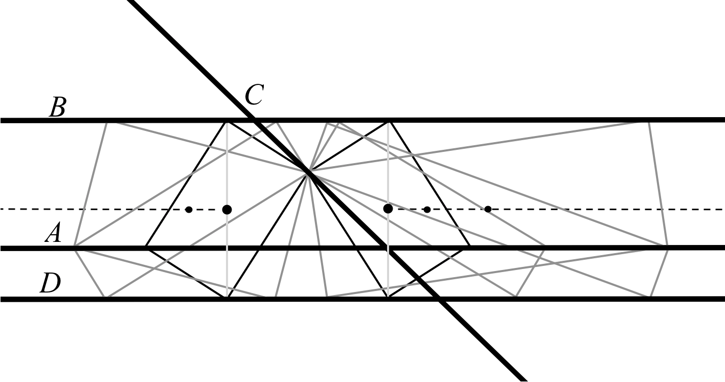
See Figure 6 for an example in which , an example that covers the case of rectangles inscribed in 3 lines.

Since degeneracy of is equivalent to the orthogonality of the diagonals and , there are many more cases of degenerate configurations than Corollary 7.3 might suggest. The next corollary shows that it is always possible to degenerate the configuration by translating one line only, and that if does not have twin pairs, there are only two such translations that work.
Corollary 7.4.
Let . If does not have twin pairs, then with fixed, there are two choices for in which is degenerate, while if is does have twin pairs, any choice of yields a degenerate configuration.
Proof.
By Theorem 7.1, is degenerate if and only if . Equivalently, using the definition of the , is degenerate if and only if is a zero of the polynomial
where A calculation shows that the discriminant of this polynomial is
which is the discriminant from the proof of Theorem 3.5. As in that proof, if , then if and only if has twin pairs. As long as does not have twin pairs, there are exactly two choices of that result in a degenerate configuration for . On the other hand, if has twin pairs, Corollary 7.3 implies is degenerate. ∎
Lemma 3.5 shows that an entire line of rectangles in may occur at infinity. If this happens, then is degenerate by Theorem 7.1. In Corollary 7.5 we distinguish when it is the slope path vs. the aspect path that occurs at infinity. By Theorem 7.1(6), the slope and aspect paths cannot both be the line at infinity for the plane of parallelograms in . See Figure 5 for two examples in which the slope path is the line at infinity.
Corollary 7.5.
The slope path is the line at infinity for the plane of parallelograms in if and only if has twin pairs, and the aspect path is the line at infinity if and only if has dual pairs.
Proof.
Suppose that the slope path is the line at infinity. By Lemma 3.5, either has twin pairs or dual pairs. Since the slope path is the line at infinity, , and so by Remark 5.3, . In this case, , so if has dual pairs, then and , so that , contrary to our standing assumption on and . Therefore, has twin pairs.
Conversely, if has twin pairs, then is degenerate by Corollary 7.3 and so the slope and aspect paths are lines by Theorem 7.1. By Lemma 3.5, one of these lines is the line at infinity for the plane of parallelograms at infinity. Since has twin pairs, examination of the coefficients of the polynomial shows that , and so every element of occurs as the slope of a rectangle at infinity by Theorem 4.5. By Theorem 7.1, every rectangle on the aspect path has the same slope, so the aspect path is not the line at infinity. Therefore, the slope path is the line at infinity.
Similarly, if the aspect path is the line at infinity, then , and Remark 6.3 implies that . Thus one of the following sets consists of parallel lines: Since is not parallel to , we have either that or . By Lemma 3.5, has twin pairs or dual pairs. Since , we cannot have that has twin pairs along with three slopes being equal, so we conclude has dual pairs.
Conversely, if has dual pairs, then is degenerate by Corollary refcases. A calculation shows that the coefficients of are . By Theorem 4.9, every element in occurs as the aspect ratio of a rectangle at infinity, so, since by Theorem 7.1 every rectangle on the aspect path has the same aspect ratio, the line at infinity is not the slope path. Therefore, the aspect path is the line at infinity. ∎
Thus if is a formally real field, the aspect path is never the line at infinity for the plane of parallelograms, and so there are at most two rectangles at infinity on the aspect path.
8. Non-degenerate configuration
Theorem 7.1(7) shows that a generic choice of the configuration —that is, a choice of for which —results in a non-degenerate configuration, and so the non-degenerate configurations present a more typical situation. Because of this, it is worthwhile to describe the behavior of the slope and aspect paths in this case too. Negations of the statements in Theorem 7.1 give useful characterizations of the non-degenerate case, but some of the ideas can be pushed a little farther to obtain stronger statements. We do this in the next theorem.
Theorem 8.1.
The following are equivalent.
- (1)
is non-degenerate.
- (2)
Every rectangle in lies on the slope path.
- (3)
Every rectangle in lies on the aspect path.
- (4)
The slope path is the aspect path.
- (5)
No two rectangles on the aspect path have the same slope.
- (6)
No two rectangles on the slope path have the same aspect ratio.
- (7)
No two rectangles in have the same slope.
- (8)
No two rectangles in have the same aspect ratio.
Proof.
To see that (1) implies (2), suppose that is non-degenerate. We use the isomorphism from the proof of Theorem 7.1 to work in instead of . By Theorem 7.1 the slope path is not a line, Let be the algebraic closure of , let be the defining equation for the image of the slope path in under , and let be the defining equation for the image in of the set of rectangles in as in Theorem 3.3. Since the image of the slope path lies in this set, the Nullstellensatz implies that is in the radical of the ideal generated by in the ring . Since a projective rational plane curve that is parameterized by polynomials has order equal to the highest degree of these polynomials [7, Exercise 3, p. 151], this implies that has degree . If is irreducible in this ring, then since has degree at most , for some . In this case, the slope path is the set of rectangles in , from which (2) follows. Otherwise, if is not irreducible, then is a product of two linear homogeneous polynomials in . It follows that for some . Thus and have the same zeroes in , which proves that the slope path is the set of rectangles in . For the proof that (1) implies (3), apply the same argument to the aspect path. It follows from this also that (1) implies (4).
That (2) implies (5) follows from the fact that every rectangle on the slope path has a different slope by Theorem 5.4. Similarly, (3) implies (6) by Theorem 6.4. Also, that (4) implies (5) follows from Theorem 5.4. That (5) and (6) each imply (1) follows from Theorem 7.1. This proves that (1)–(6) are equivalent. That (4) implies (7) and (8) follows from the already established fact that (4) implies (5) and (6). Also, (7) and (8) each imply (1) by Theorem 7.1, so (1)–(8) are equivalent. ∎
Figure 1 illustrates Theorem 8.1. With the theorem, we can show finally that the slope and aspect paths find all rectangles in .
Corollary 8.2.
Every rectangle in lies on the slope path or the aspect path.
Proof.
We show next that if is non-degenerate, the slope and aspect paths are computable from each other by factoring through a homography, and so the aspect ratio of a rectangle in depends entirely on its slope, and vice versa, slope is determined by aspect ratio. Theorem 7.1 shows this is only true for the non-degenerate case.
Theorem 8.3.
If is non-degenerate, then the slope path is the aspect path composed with a homography . The aspect path is the slope path composed with .
Proof.
First we show there is a homography such that a rectangle in has slope if and only if its aspect ratio is . Define for all by and Theorem 7.1 implies that is non-degenerate if and only if , and so , , and . A simple calculation shows that is the inverse of . By Theorem 5.4, for each , is the aspect ratio of the rectangle on the slope path that has slope , and by Theorem 6.4, is the slope of the rectangle on the aspect path that has aspect ratio .
Let denote the slope and aspect paths from Theorems 5.4 and 6.4, and let be the homography from Theorem 8.3. Let . By Theorem 6.4 and the fact that , we have that is a rectangle with slope . By Theorem 5.4, also is a rectangle in with slope , and so by Theorem 8.1. This shows that . Since is a homography, . ∎
9. Rectangle locus
In this section, because we work with midpoints, we assume is a field of characteristic other than . It is sometimes useful to have a direct way of representing rectangles in with a point in rather than . In [4] and [6], this is done for the case using the rectangle locus of the configuration, the set of centers of the rectangles in . If neither of the pairs of lines in the configuration consists of parallel lines, then each point on the rectangle locus uniquely determines a rectangle inscribed in sequence in the lines , and so the rectangle locus gives a good way to track the path of inscribed rectangles through the configuration. It is shown in [4] and [6] that in the case in which and neither pair nor consists of parallel or perpendicular lines, the rectangle locus is a hyperbola. See Figures 1 and 2 for examples of this. However, if at least one of the pairs consists of parallel lines or both pairs consist of perpendicular lines, then the locus can be a line, a line with a segment missing, or a point; see [4, Section 4]. Figures 7 and 8 illustrate two such cases.

Theorem 3.6 helps explain these observations. This is because there is a linear transformation from to that sends a rectangle to its center, and the rectangle locus is the image under this transformation of either a line or a plane curve of degree . If , then by Theorem 3.6 the rectangle locus is the image of either a line or a planar hyperbola, and if no pairs among are parallel or orthogonal, then the rectangle locus is a hyperbola. (With the assumption of no parallel lines, it is straightforward to see that this linear transformation restricts to a bijection from the set of rectangles in to the rectangle locus for .)
For the rest of the section we work under the assumption that none of are parallel, and we interpret the rectangle locus and rectangles at infinity for the case in which is degenerate. With degenerate, the rectangle locus is by Theorem 7.1 a pair of lines, one the image of the slope path and the other the image of the aspect path. We say that the image of the slope path is the slope path of centers for and the image of the aspect path is the aspect path of centers for . The slope path of centers is the image of the linear transformation from to that sends a rectangle to its center composed with the slope path, and so it sends to the center of a rectangle in with slope . A similar statement holds for the aspect path of centers.
Let denote the intersection of the lines and , the intersection of and , etc.. If , then the midpoints of the traditional diagonals of the complete quadrilateral formed by lie on a line, the Gauss-Newton line. It is straightforward to see that this remains true for any choice of field with characteristic other than ; i.e., the following points are collinear:
We refer to the line through these three points as the Gauss-Newton line. Also, for the purpose of stating the next theorem, we denote by the third diagonal of the configuration , that is, the line through the points and . (Recall that is the line through and and is the line through and .)
Theorem 9.1.
Suppose is a degenerate configuration in which no lines are parallel. Then the aspect path of centers is the Gauss-Newton line. If at least one of the pairs or is not orthogonal, the slope path of centers is a line that is parallel to the diagonal .
Proof.
By Theorem 7.1, the slope and aspect paths are lines, so the slope and aspect paths of centers are lines too. The points and are the vertices of a degenerate rectangle in with slope that is orthogonal to the slope of , the line that passes through them. Similarly, and , which lie on , are the vertices of a degenerate rectangle in with slope equal to , the slope of . Since is orthogonal to by Theorem 7.1, these two degenerate rectangles have slope .
We claim these two rectangles lie on the aspect path. By Theorem 7.1, every rectangle on the aspect path, including the rectangle at infinity, has slope , and so by Theorem 4.5, the other rectangle at infinity has slope equal to the slope of . By Theorem 5.4, no two rectangles on the slope path have the same slope, so there is at most one rectangle on the slope path with slope . The point of intersection of the slope path and aspect path is a rectangle having slope , so since every rectangle occurs on the slope path or the aspect path by Corollary 8.2, both of these degenerate rectangles lie on the aspect path, and hence their centers, which are the midpoints of the degenerate rectangles, lie on the aspect path of centers. Since this path is a line, it is the Gauss-Newton line.
To prove the second claim of the theorem, suppose that at least one of the pairs and is not orthogonal. By Lemma 2.4 the slope of the diagonal is . We have observed already that there are two rectangles at infinity, one having the slope of and the other the slope of , and that the rectangle at infinity for the aspect path has slope equal to the slope of . Thus the rectangle at infinity for the slope path has slope . By Theorem 4.5, , and by Theorem 5.4, the rectangle at infinity on the slope path is
The center of this rectangle is
Since this rectangle is the point at infinity for the slope path of centers, the slope of the line that is the slope path of centers is
Since is degenerate and , we have and or , whichever is defined. Since , regardless of whichever of these fractions is defined, we have . Calculating, we see
Similarly, since , we have
The lines and the lines intersect, respectively, in the two points
so the slope of the diagonal is which is the same as the slope of the slope path of centers. ∎
The restriction in the theorem that at least one of the pairs and is not orthogonal is necessary. Otherwise, has twin pairs and the slope path is the line at infinity (Corollary 7.5), and so the slope path is not parallel to .
We next interpret the rectangles at infinity for a degenerate configuration. To do so, it suffices to describe the slope and aspect ratio of these rectangles since this information uniquely determines the rectangle up to scale. The four points of intersection defined above are the vertices of a quadrilateral, and it is straightforward to see that the midpoints of adjacent “sides” form the vertices of a parallelogram. (In the case , this is known as the Varignon parallelogram of the quadrilateral.) The center of the parallelogram is the centroid of . The diagonals and are orthogonal if and only if this parallelogram is a rectangle.
Definition 9.2.
Suppose is a degenerate configuration in which no lines are parallel. The center rectangle is the rectangle in whose center is the intersection of the two lines that comprise the rectangle locus. The centroid rectangle is the rectangle in whose center is the centroid of .

Theorem 9.3.
Suppose is a degenerate configuration in which no lines are parallel. The rectangle at infinity for the slope path has the aspect ratio of the center rectangle and is orthogonal to it, while the rectangle at infinity for the aspect path has the slope of the centroid rectangle and aspect ratio the negative of the aspect ratio of the centroid rectangle.
The theorem is more easily stated in the case : The rectangle at infinity for the slope path is the center rectangle with a quarter turn, while the rectangle at infinity for the aspect path is the centroid rectangle flipped and inscribed in the opposite of whichever direction, clockwise or counterclockwise, the centroid rectangle is inscribed.
Proof.
As in the proof of Theorem 9.1, the rectangle at infinity for the aspect path has slope and the rectangle at infinity for the slope path has slope equal to the slope of . Also by Theorem 7.1, every rectangle on the slope path has the same aspect ratio, so the rectangle at infinity for the slope path has the same aspect ratio as the center rectangle and is orthogonal to it. The aspect ratio of the centroid rectangle is
Using the calculation of these vertices from the proof of Lemma 2.4, we have
Therefore, the aspect ratio of the centroid is By Theorem 5.4, the aspect ratio of the rectangle at infinity for the slope path is . By Remark 4.10, is the aspect ratio of the rectangle at infinity for the aspect path, and this is the negative of the aspect ratio of the centroid rectangle. ∎

Remark 9.4.
As discussed in the introduction, our approach throughout the paper assumes that at least two lines in a configuration are not parallel. The situation in which all four lines are parallel and the field does not have characteristic can be described as follows. If the pairs and do not share the same midline (i.e., the line consisting of midpoints of the points on either line), then there are no rectangles inscribed in . Otherwise, if the pairs share the same midline, then the midline is the rectangle locus, and for each choice of with , there is a unique rectangle inscribed in whose vertices on and are and . Therefore, the “curve” of rectangles for this configuration is not a curve at all but a surface in parameterized by the points in In any case, this accounts for all the rectangles inscribed in . Figure 10 illustrates this situation.
References
- [1] A. Emch, On some properties of the medians of closed continuous curves formed by analytic arcs, Amer. J. Math. 38 (1916), 6–18.
- [2] I. Kaplansky, Linear algebra and geometry: a second course, Dover, 2003.
- [3] M. D. Meyerson, Balancing acts, Topology Proc. 6 (1981), 59–75.
- [4] B. Olberding and E. A. Walker, The conic geometry of rectangles inscribed in lines, Proc. Amer. Math. Soc., to appear, arXiv:1908.05413.
- [5] P. Samuel, Projective geometry, Springer, 1988.
- [6] R. Schwartz, Four lines and a rectangle, Exper. Math. (2020), DOI: 10.1080/10586458.2019.1671923.
- [7] R. J. Walker, Algebraic curves, Dover, New York, 1962.