跳到论文正文
W Papers独立论文阅读器 arXiv:2006.14325 论文正文 计算阅读时间 · 0%
引用这篇论文根据当前论文元数据生成,正式投稿前建议核对。


License: arXiv.org perpetual non-exclusive license
arXiv:2006.14325v1 [cs.LG] 25 Jun 2020

High-Dimensional Quadratic Discriminant Analysis
under Spiked Covariance Model

Houssem Sifaou       Abla Kammoun    and Mohamed-Slim Alouini    Thanks: H. Sifaou, A. Kammoun and M.S. Alouini are with the Computer, Electrical, and Mathematical Sciences and Engineering (CEMSE) Division, KAUST, Thuwal, Makkah Province, Saudi Arabia (e-mail: houssem.sifaou@kaust.edu.sa, abla.kammoun@kaust.edu.sa, slim.alouini@kaust.edu.sa).
Abstract

Quadratic discriminant analysis (QDA) is a widely used classification technique that generalizes the linear discriminant analysis (LDA) classifier to the case of distinct covariance matrices among classes. For the QDA classifier to yield high classification performance, an accurate estimation of the covariance matrices is required. Such a task becomes all the more challenging in high dimensional settings, wherein the number of observations is comparable with the feature dimension. A popular way to enhance the performance of QDA classifier under these circumstances is to regularize the covariance matrix, giving the name regularized QDA (R-QDA) to the corresponding classifier. In this work, we consider the case in which the population covariance matrix has a spiked covariance structure, a model that is often assumed in several applications. Building on the classical QDA, we propose a novel quadratic classification technique, the parameters of which are chosen such that the fisher-discriminant ratio is maximized. Numerical simulations show that the proposed classifier not only outperforms the classical R-QDA for both synthetic and real data but also requires lower computational complexity, making it suitable to high dimensional settings.

Index Terms: 
High-Dimensional Data, Quadratic Discriminant Analysis, Random Matrix Theory, Spiked Covariance Models.

I Introduction

Classification is among the most typical examples of supervised learning techniques. When the data is normally distributed with common covariance matrices across classes, linear discriminant analysis (LDA) is known to be the optimal classifier in terms of misclassification rate minimization. In the case of different covariances across classes, it has recently been shown that the use of LDA does not enable to leverage the information on the differences between covariance matrices [1]. Under such circumstances, it can be more advisable to employ the quadratic discriminant analysis (QDA), which turns out to be the optimal classifier under Gaussian data and known statistics. In practical scenarios, the covariance matrices and the means associated with each class are not perfectly known. They are often estimated based on the available training data for which the class label associated with each observation is provided. If the number of training samples nn and their dimensions pp are commensurable, a situation widely met in numerous applications such as medical imaging [2], functional data analysis [3], meteorology and oceanography [4], many estimators of the covariance matrices such as the sample covariance matrix become highly inaccurate. A typical extreme scenario corresponds to the case n<pn<p, in which the sample covariance matrix becomes singular, and as such, cannot be used as a plug-in estimator of the covariance matrix since the QDA classifier involves the computation of the inverse covariance matrix. To get around this issue, it was proposed to use instead, a regularized covariance matrix estimator that linearly shrinks through the use of a scalar regularization parameter the sample covariance matrix towards identity [5]. The corresponding classifier is referred to as regularized QDA (R-QDA). This regularization appoach has been used succefully in several applications [6, 7, 8]. However, QDA and R-QDA remain widely unused in high-dimensional settings, being very sensitive to the estimation quality of the covariance matrix [9].

In this work, we consider a high-dimensional setting in which the number of observations is assumed to scale with their dimensions. We further assume that the population covariance matrix associated with each class is a low-rank perturbation of a scaled identity; that is, it is isotropic except for a finite number of symmetry-breaking directions. Such a model is used in many real applications such as detection[10], electroencephalogram (EEG) signals[11, 12], and financial econometrics[13, 14], and is known in the random matrix theory terminology as the spiked covariance model. Based on this model, we propose to employ for each class a parametrized covariance matrix estimator following the same model as the population covariance matrix. The parameters correspond to the largest eigenvalues, which are optimized to maximize the classifier performance. More specifically, by leveraging tools from random matrix theory, we compute the asymptotic Fisher ratio in the regime nn and pp growing to infinity at the same pace. Closed-form expressions of the optimal parameters that maximize the asymptotic Fisher ratio are then provided. The approach consisting of exploiting the spiked structure of the covariance matrix has mainly been considered in signal processing applications [15] and [16]. It has only recently been used for the classification problem in our work in [17, 18], wherein a similar approach is applied to find an improved LDA classifier under the spiked covariance model assumption. Considering a QDA based classifier is needed when the covariance matrices between classes are different. It is also more challenging since it involves an involved quadratic statistic, the statistical properties of which are much harder to characterize.

The proposed classifier is compared with the regularized QDA (R-QDA) classifier [5] using both real and synthetic data. The proposed classifier outperforms the classical R-QDA classifier while requiring less computational complexity. As shown next in the paper, the proposed classifier involves a statistic that avoids computing the inverse of the covariance matrix. Moreover, since the parameters are obtained in closed-form, it avoids the grid search or the cross-validation approach needed to determine the optimal regularization parameter of the R-QDA classifier[5].

The remainder of this paper is organized as follows. In the next section, a brief overview of QDA and R-QDA classifiers is provided. Section III details the steps of the design of our proposed classifier. The performance of the proposed classifier is studied in section IV, and some concluding remarks are drawn in section V.

I-A Notations

Throughout this work, boldface lower case is used for denoting column vectors, 𝐱{\bf x}, and upper case for matrices, 𝐗{\bf X}. 𝐗T{\bf X}^{T} denotes the transpose. Moreover, 𝐈p{\bf I}_{p}, 𝟎p\boldsymbol{0}_{p} and 𝟏p\boldsymbol{1}_{p} denote the identity matrix, the all-zero vector and all-one vector of size pp respectively. |𝐗|\left|{\bf X}\right| and tr⁡(𝐗)\tr\left({\bf X}\right) denote the determinant and the trace of 𝐗{\bf X} respectively. {xj}j=1r\left\{x_{j}\right\}_{j=1}^{r} is used to denote the row vector with entries xjx_{j} whereas ∥.∥\|.\| is used to denote the ℓ2\ell_{2}-norm. The almost sure convergence and the convergence in distribution of random variables will be denoted as ⟶a.s.\overset{a.s.}{\longrightarrow} and ⟶𝑑\overset{d}{\longrightarrow} receptively.

II Quadratic Discriminant Analysis

Consider 𝐱1,⋯,𝐱n{\bf x}_{1},\cdots,{\bf x}_{n} observations of size pp belonging to two different classes 𝒞0\mathcal{C}_{0} and 𝒞1\mathcal{C}_{1} with nin_{i} observations belonging to class 𝒞i\mathcal{C}_{i}. For notational convenience, we denote by 𝒯i\mathcal{T}_{i} the set of indexes of the observations belonging to class 𝒞i\mathcal{C}_{i}. We assume that 𝐱ℓ∈𝒞i,i∈{0,1}{\bf x}_{\ell}\in\mathcal{C}_{i},i\in\{0,1\}, is drawn from a Gaussian distribution with mean 𝝁i\boldsymbol{\mu}_{i} and covariance 𝚺i\boldsymbol{\Sigma}_{i}. In this work, a ’spiked model’ is assumed for the covariance matrices. Under this assumption, for i∈{0,1}i\in\left\{0,1\right\}, 𝚺i\boldsymbol{\Sigma}_{i} is written as:

𝚺i=σi2​𝐈p+σi2​∑j=1riλj,i​𝐯j,i​𝐯j,iT,\boldsymbol{\Sigma}_{i}=\sigma_{i}^{2}{\bf I}_{p}+\sigma_{i}^{2}\sum_{j=1}^{r_{i}}\lambda_{j,i}{\bf v}_{j,i}{\bf v}_{j,i}^{T}, (1)

where σi2>0\sigma_{i}^{2}>0, λ1,i≥⋯,≥λri,i>0\lambda_{1,i}\geq\cdots,\geq\lambda_{r_{i},i}>0 and 𝐯1,i,⋯,𝐯ri,i{\bf v}_{1,i},\cdots,{\bf v}_{r_{i},i} are orthonormal.

Remark.

The assumed model of the covariance matrices is encountered in many real applications such as detection[10], EEG signals[11, 12], and financial econometrics[13, 14].

The starting point of our work is the classical QDA classifier whose discriminant function is given by:

WQDA​(𝐱)\displaystyle W^{\rm QDA}({\bf x}) =ηQDA−12​(𝐱−𝝁0)T​𝚺0−1​(𝐱−𝝁0)+12​(𝐱−𝝁1)T​𝚺1−1​(𝐱−𝝁1),\displaystyle=\eta^{\rm QDA}-\frac{1}{2}({\bf x}-\boldsymbol{\mu}_{0})^{T}\boldsymbol{\Sigma}_{0}^{-1}({\bf x}-\boldsymbol{\mu}_{0})+\frac{1}{2}({\bf x}-\boldsymbol{\mu}_{1})^{T}\boldsymbol{\Sigma}_{1}^{-1}({\bf x}-\boldsymbol{\mu}_{1}), (2)

where ηQDA=−12​log⁡|𝚺0||𝚺1|−log⁡π1π0\eta^{\rm QDA}=-\frac{1}{2}\log\frac{|\boldsymbol{\Sigma}_{0}|}{|\boldsymbol{\Sigma}_{1}|}-\log\frac{\pi_{1}}{\pi_{0}} and πi\pi_{i} is the prior probability for class 𝒞i\mathcal{C}_{i}. An observation 𝐱{\bf x} is classified to 𝒞0\mathcal{C}_{0} if the discriminant function WQDA​(𝐱)W^{\rm QDA}({\bf x}) is positive and to class 𝒞1\mathcal{C}_{1} otherwise. In practice, the mean vectors and covariance matrices are unknown and are usually replaced by their empirical estimates. For notational convenience, we define the sample mean and the sample covariance matrix of class i∈{0,1}i\in\left\{0,1\right\}, respectively as:

𝐱¯i=1ni​∑ℓ∈𝒯i𝐱ℓ,\displaystyle\overline{{\bf x}}_{i}=\frac{1}{n_{i}}\sum_{\ell\in\mathcal{T}_{i}}{\bf x}_{\ell},
𝚺^i=1ni−1​∑ℓ∈𝒯i(𝐱ℓ−𝐱¯i)​(𝐱ℓ−𝐱¯i)T.\displaystyle\hat{\boldsymbol{\Sigma}}_{i}=\frac{1}{n_{i}-1}\sum_{\ell\in\mathcal{T}_{i}}({\bf x}_{\ell}-\overline{{\bf x}}_{i})({\bf x}_{\ell}-\overline{{\bf x}}_{i})^{T}.

It is the case in many real data sets that the dimension of the observations is of the same order of magnitude if not higher than their numbers, which makes the sample covariance matrix 𝚺^i\hat{\boldsymbol{\Sigma}}_{i} ill-conditioned. To overcome this issue, ridge estimators of the inverse of the covariance matrix are used [19, 9]:

𝐇i=(𝐈p+γ​𝚺^i)−1,γ>0.{\bf H}_{i}=\left({\bf I}_{p}+\gamma\hat{\boldsymbol{\Sigma}}_{i}\right)^{-1},\ \ \gamma>0. (3)

Replacing 𝚺i\boldsymbol{\Sigma}_{i} by 𝐇i{\bf H}_{i} into (2) yields the R-QDA classifier, the statistic of which is given by:

W^R−QDA​(𝐱)\displaystyle\hat{W}^{\rm R-QDA}({\bf x}) =ηR−QDA−12​(𝐱−𝐱¯0)T​𝐇0−1​(𝐱−𝐱¯0)+12​(𝐱−𝐱¯1)T​𝐇1−1​(𝐱−𝐱¯1),\displaystyle=\eta^{\rm R-QDA}-\frac{1}{2}({\bf x}-\overline{{\bf x}}_{0})^{T}{\bf H}_{0}^{-1}({\bf x}-\overline{{\bf x}}_{0})+\frac{1}{2}({\bf x}-\overline{{\bf x}}_{1})^{T}{\bf H}_{1}^{-1}({\bf x}-\overline{{\bf x}}_{1}), (4)

where ηR−QDA=−12​log⁡|𝐇1||𝐇0|−log⁡π1π0\eta^{\rm R-QDA}=-\frac{1}{2}\log\frac{|{\bf H}_{1}|}{|{\bf H}_{0}|}-\log\frac{\pi_{1}}{\pi_{0}}. The classification error of R-QDA corresponding to class ii can be written as,

ϵiR−QDA\displaystyle\epsilon^{\rm R-QDA}_{i} =ℙ⁡[(−1)i​W^R−QDA​(𝐱)<0|𝐱∈𝒞i],\displaystyle=\mathbb{P}\left[(-1)^{i}\hat{W}^{\rm R-QDA}({\bf x})<0|{\bf x}\in\mathcal{C}_{i}\right],

The global classification error is given by,

ϵR−QDA=π0​ϵ0R−QDA+π1​ϵ1R−QDA.\epsilon^{\rm R-QDA}=\pi_{0}\epsilon^{\rm R-QDA}_{0}+\pi_{1}\epsilon^{\rm R-QDA}_{1}. (5)

The optimal parameter of R-QDA classifier γ∗\gamma^{*}, that minimizes the global classification error, is generally computed by comparing the performance of a few candidate values using a cross-validation method [5].

III Improved QDA

III-A Proposed classification rule

In this section, we propose an improved QDA classifier that leverages the structure of the covariance matrix model in (1). For simplicity, we assume that σi2\sigma_{i}^{2} and rir_{i} are perfectly known. In practice, there exist several efficient algorithms in the literature for the estimation of these parameters. For more details, we refer the reader to the following works [14, 20, 21, 13].

Let 𝚺^i=∑j=1psj,i​𝐮j,i​𝐮j,iT,\hat{\boldsymbol{\Sigma}}_{i}=\sum_{j=1}^{p}s_{j,i}{\bf u}_{j,i}{\bf u}_{j,i}^{T}, be the eigenvalue decomposition of the sample covariance matrix corresponding to class ii, with sj,is_{j,i} is the jj-th largest eigenvalue of 𝚺^i\hat{\boldsymbol{\Sigma}}_{i} and 𝐮j,i{\bf u}_{j,i} its corresponding eigenvector. We look for an inverse covariance matrix estimator that possesses the same eigenvector basis. It can be thus written as:

𝐂^i−1=∑j=1ptj,i​𝐮j,i​𝐮j,iT,\hat{\bf C}_{i}^{-1}=\sum_{j=1}^{p}t_{j,i}{\bf u}_{j,i}{\bf u}_{j,i}^{T},

where tj,it_{j,i} are some parameters to be designed. In accordance with the covariance matrix model in (1), it is natural to set tp−r,i=⋯=tp,i=1/σi2t_{p-r,i}=\cdots=t_{p,i}=1/\sigma_{i}^{2}. Such operation allows to shrink the covariance matrix estimator towards the structure described by (1), giving it the name of a shrinkage estimator [22]. Thus, the inverse of the covariance matrix can be estimated as,

𝐂^i−1=1σi2​(𝐈p+∑j=1riwj,i​𝐮j,i​𝐮j,iT),\hat{\bf C}_{i}^{-1}=\frac{1}{\sigma_{i}^{2}}\left({\bf I}_{p}+\sum_{j=1}^{r_{i}}w_{j,i}{\bf u}_{j,i}{\bf u}_{j,i}^{T}\right), (6)

where wj,i=σi2​tj,i−1w_{j,i}=\sigma_{i}^{2}t_{j,i}-1. In the sequel, we work with wj,iw_{j,i} as the considered optimization variables. For notational convenience, we define 𝐰=[w1,1,⋯,wr1,1,w1,0,⋯,wr0,0]T{\bf w}=[w_{1,1},\cdots,w_{r_{1},1},w_{1,0},\cdots,w_{r_{0},0}]^{T}. Our analysis relies on an asymptotic analysis of the behavior of the proposed QDA classifier. The asymptotic regime that is considered in our work is described in the following assumption:

Assumption 1.

Throughout this work, we assume that, for i∈{0,1}i\in\left\{0,1\right\},

  • (i) ni,p​⟶a.s.​∞n_{i},p\overset{a.s.}{\longrightarrow}\infty, with fixed ratio ci=p/nic_{i}=p/n_{i}.

  • (ii) rir_{i} is fixed and λ1,i>⋯>λri,i>ci\lambda_{1,i}>\cdots>\lambda_{r_{i},i}>\sqrt{c_{i}}, independently of pp and nin_{i}.

  • (iii) The spectral norm of 𝚺i\boldsymbol{\Sigma}_{i}, ‖𝚺i‖\|\boldsymbol{\Sigma}_{i}\| are bounded, that is ‖𝚺i‖=O⁡(1)\|\boldsymbol{\Sigma}_{i}\|=O(1).

  • (iv) The mean difference vector 𝝁≜𝝁1−𝝁0\boldsymbol{\mu}\triangleq\boldsymbol{\mu}_{1}-\boldsymbol{\mu}_{0} has a bounded Euclidean norm, that is ‖𝝁‖=O⁡(1)\|\boldsymbol{\mu}\|=O(1).

  • (v) σi2=O⁡(1)\sigma_{i}^{2}=O(1) and σ02−σ12=O⁡(1/p)\sigma_{0}^{2}-\sigma_{1}^{2}=O(1/p).

Remark.
  • •

    Assumption (i) is a key assumption that is generally in the framework of the theory of large random matrices.

  • •

    Assumption (ii) is fundamental in our analysis since it guarantees, as per standard results from random matrix theory, the one-to-one mapping between the sample eigenvalues sj,is_{j,i} and the unknown λj,i\lambda_{j,i}. In fact, when λj,i>ci\lambda_{j,i}>\sqrt{c_{i}}, λj,i\lambda_{j,i} can be consistently estimated using sj,is_{j,i} as we will see later. In the case where λj,i≤ci\lambda_{j,i}\leq\sqrt{c_{i}}, the relation between sj,is_{j,i} and λj,i\lambda_{j,i} no longer holds and λj,i\lambda_{j,i} cannot be estimated [23, 24].

  • •

    Assumption (v) is a technical assumption, under which tr⁡(𝚺1−𝚺0)=O⁡(1)\tr\left(\boldsymbol{\Sigma}_{1}-\boldsymbol{\Sigma}_{0}\right)=O(1). Moreover, from (1), it ensures that the low-rank perturbation in 𝚺i\boldsymbol{\Sigma}_{i} has a non-negligible contribution in tr⁡(𝚺1−𝚺0)\tr\left(\boldsymbol{\Sigma}_{1}-\boldsymbol{\Sigma}_{0}\right). This is a key assumption that is needed for the parameter vector 𝐰{\bf w} to be asymptotically relevant for the classification.

Using the proposed covariance estimator, the discriminant function associated with the proposed classifier is given as:

W^Imp−QDA​(𝐱)=\displaystyle\hat{W}^{\rm Imp-QDA}({\bf x})= η−12​(𝐱−𝝁0)T​𝐂^0−1​(𝐱−𝝁0)+12​(𝐱−𝝁1)T​𝐂^1−1​(𝐱−𝝁1),\displaystyle\eta-\frac{1}{2}({\bf x}-\boldsymbol{\mu}_{0})^{T}\hat{\bf C}_{0}^{-1}({\bf x}-\boldsymbol{\mu}_{0})+\frac{1}{2}({\bf x}-\boldsymbol{\mu}_{1})^{T}\hat{\bf C}_{1}^{-1}({\bf x}-\boldsymbol{\mu}_{1}), (7)

where η\eta accounts for an additional bias; the way it is selected will be shown later. Let 𝐱{\bf x} be a testing observation belonging to class 𝒞i\mathcal{C}_{i}. Then, 𝐱=𝝁i+𝚺i12​𝐳{\bf x}=\boldsymbol{\mu}_{i}+\boldsymbol{\Sigma}_{i}^{\frac{1}{2}}{\bf z} with 𝐳∼𝒩⁡(𝟎,𝐈p){\bf z}\sim\mathcal{N}({\bf 0},{\bf I}_{p}). The classification error corresponding to class 𝒞i\mathcal{C}_{i} can be written as,

ϵiImp−QDA\displaystyle\epsilon^{\rm Imp-QDA}_{i} =ℙ⁡[(−1)i​W^Imp−QDA​(𝐱)<0|𝐱∈𝒞i],\displaystyle=\mathbb{P}\left[(-1)^{i}\hat{W}^{\rm Imp-QDA}({\bf x})<0|{\bf x}\in\mathcal{C}_{i}\right], (8)
=ℙ⁡[(−1)i​Yi​(𝐂^0,𝐂^1)<0|𝐳∼𝒩⁡(𝟎,𝐈p)],\displaystyle=\mathbb{P}\left[(-1)^{i}Y_{i}(\hat{\bf C}_{0},\hat{\bf C}_{1})<0|{\bf z}\sim\mathcal{N}(\boldsymbol{0},{\bf I}_{p})\right], (9)

where

Yi​(𝐂^0,𝐂^1)=𝐳T​𝐁i​𝐳+2​𝐲iT​𝐳−ξi,Y_{i}(\hat{\bf C}_{0},\hat{\bf C}_{1})={\bf z}^{T}{\bf B}_{i}{\bf z}+2{\bf y}_{i}^{T}{\bf z}-\xi_{i}, (10)

with

𝐁i=\displaystyle{\bf B}_{i}= 𝚺i12​(𝐂^1−1−𝐂^0−1)​𝚺i12,\displaystyle\boldsymbol{\Sigma}_{i}^{\frac{1}{2}}\left(\hat{\bf C}_{1}^{-1}-\hat{\bf C}_{0}^{-1}\right)\boldsymbol{\Sigma}_{i}^{\frac{1}{2}},
𝐲i=\displaystyle{\bf y}_{i}= 𝚺i12​[𝐂^1−1​(𝝁i−𝐱¯1)−𝐂^0−1​(𝝁i−𝐱¯0)],\displaystyle\boldsymbol{\Sigma}_{i}^{\frac{1}{2}}\left[\hat{\bf C}_{1}^{-1}(\boldsymbol{\mu}_{i}-\overline{{\bf x}}_{1})-\hat{\bf C}_{0}^{-1}(\boldsymbol{\mu}_{i}-\overline{{\bf x}}_{0})\right],
ξi=\displaystyle\xi_{i}= −2​η+(𝝁i−𝐱¯0)T​𝐂^0−1​(𝝁i−𝐱¯0)−(𝝁i−𝐱¯1)T​𝐂^1−1​(𝝁i−𝐱¯1),\displaystyle-2\eta+(\boldsymbol{\mu}_{i}-\overline{{\bf x}}_{0})^{T}\hat{\bf C}_{0}^{-1}(\boldsymbol{\mu}_{i}-\overline{{\bf x}}_{0})-(\boldsymbol{\mu}_{i}-\overline{{\bf x}}_{1})^{T}\hat{\bf C}_{1}^{-1}(\boldsymbol{\mu}_{i}-\overline{{\bf x}}_{1}),
Proposition 1.

Under the conditions (i){\it(i)}, (𝑖𝑖𝑖){\it(iii)} and (v){\it(v)} of Assumption 1, we have

Yi​(𝐂^0,𝐂^1)−Y~i​⟶𝑑​0\displaystyle Y_{i}(\hat{\bf C}_{0},\hat{\bf C}_{1})-\tilde{Y}_{i}\overset{d}{\longrightarrow}0

where

Y~i=p​σi2​(1σ12−1σ02)+νi+2​𝐲iT​𝐳−ξi,\displaystyle\tilde{Y}_{i}=p\sigma_{i}^{2}\left(\frac{1}{\sigma_{1}^{2}}-\frac{1}{\sigma_{0}^{2}}\right)+\nu_{i}+2{\bf y}_{i}^{T}{\bf z}-\xi_{i},

with νi=1σ12​∑j=1r1wj,1​(𝐳~iT​𝐮j,1)2−1σ02​∑j=1r0wj,0​(𝐳~iT​𝐮j,0)2\nu_{i}=\frac{1}{\sigma_{1}^{2}}\sum_{j=1}^{r_{1}}w_{j,1}(\tilde{\bf z}_{i}^{T}{\bf u}_{j,1})^{2}-\frac{1}{\sigma_{0}^{2}}\sum_{j=1}^{r_{0}}w_{j,0}(\tilde{\bf z}_{i}^{T}{\bf u}_{j,0})^{2} and 𝐳~i=𝚺i12​𝐳\tilde{\bf z}_{i}=\boldsymbol{\Sigma}_{i}^{\frac{1}{2}}{\bf z}.

It entails from Proposition 1 that the asymptotic behavior of Yi​(𝐂^0,𝐂^1)Y_{i}(\hat{\bf C}_{0},\hat{\bf C}_{1}) corresponds to that of a linear combination of a chi-squared and normal distributions. For illustration, we plot in Fig. 1 the empirical distributions of Y0​(𝐂^0,𝐂^1)Y_{0}(\hat{\bf C}_{0},\hat{\bf C}_{1}) and Y1​(𝐂^0,𝐂^1)Y_{1}(\hat{\bf C}_{0},\hat{\bf C}_{1}) built based on several testing vectors drawn from 𝒞0\mathcal{C}_{0} and 𝒞1\mathcal{C}_{1}. Unfortunately. the distribution of Yi{Y}_{i} does not have closed form expressions, which makes the analysis of the misclassification rate cumbersome.
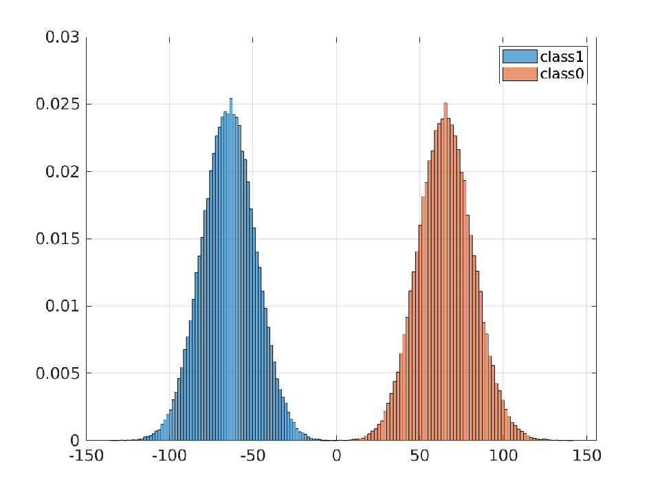
Refer to caption
Fig. 1: Histograms of Y0​(𝐂^0,𝐂^1)Y_{0}(\hat{\bf C}_{0},\hat{\bf C}_{1}) and Y1​(𝐂^0,𝐂^1)Y_{1}(\hat{\bf C}_{0},\hat{\bf C}_{1}) with synthetic data with σ02=σ12=1\sigma_{0}^{2}=\sigma_{1}^{2}=1, r0=r1=3r_{0}=r_{1}=3, λ1,0=λ1,1=4\lambda_{1,0}=\lambda_{1,1}=4, λ2,0=λ2,1=3\lambda_{2,0}=\lambda_{2,1}=3, λ3,0=λ3,1=2\lambda_{3,0}=\lambda_{3,1}=2 and 𝝁0=−𝝁1=4p​𝟏p\boldsymbol{\mu}_{0}=-\boldsymbol{\mu}_{1}=\frac{4}{\sqrt{p}}\boldsymbol{1}_{p}.

III-B Parameter optimization

In this section, we present a possible setting of the parameter vector 𝐰{\bf w}. Since the misclassification rate cannot be characterized in closed-form, we propose instead for tractability to maximize the Fisher ratio metric. Such a metric quantifies the separability between the two classes, by measuring the ratio of the separation between the means to the variance within classes and has been fundamental in the design of the Fisher discriminant analysis (FDA) based classifier. Under our setting, the square root of the Fisher-Ratio [25] associated with the classifier in (2) is given by:

ρ⁡(𝐰)=|m0​(𝐰)−m1​(𝐰)|v0​(𝐰)+v1​(𝐰),\rho({\bf w})=\frac{\left|m_{0}({\bf w})-m_{1}({\bf w})\right|}{\sqrt{v_{0}({\bf w})+v_{1}({\bf w})}},

where for i∈{0,1}i\in\left\{0,1\right\}, mi​(𝐰)m_{i}({\bf w}) and vi​(𝐰)v_{i}({\bf w}) are respectively the mean and the variance of Y~i\tilde{Y}_{i} with respect to 𝐳{\bf z}, given by:

mi​(𝐰)\displaystyle m_{i}({\bf w}) =p​σi2​(1σ12−1σ02)+𝔼​νi−ξi,\displaystyle=p\sigma_{i}^{2}\left(\frac{1}{\sigma_{1}^{2}}-\frac{1}{\sigma_{0}^{2}}\right)+\mathbb{E}\nu_{i}-\xi_{i},
vi​(𝐰)\displaystyle v_{i}({\bf w}) =var⁡(νi)+4​𝐲iT​𝐲i.\displaystyle=\var(\nu_{i})+4{\bf y}_{i}^{T}{\bf y}_{i}.

where we have used the fact that νi\nu_{i} and 𝐲iT​𝐳{\bf y}_{i}^{T}{\bf z} are uncorrelated. Following the same methodology in the design of FDA, we propose to select 𝐰{\bf w} that solves the following optimization problem:

𝐰⋆=argmax𝐰ρ⁡(𝐰).{\bf w}^{\star}=\underset{{\bf w}}{\rm argmax}\ \ \ \rho({\bf w}).

The optimization cannot be performed at this stage since mi​(𝐰)m_{i}({{\bf w}}) and vi​(𝐰)v_{i}({\bf w}) involve unknown quantities such as λj,i\lambda_{j,i} and 𝐯j,i{\bf v}_{j,i} that appear in 𝚺i\boldsymbol{\Sigma}_{i}. To overcome this issue, we resort to techniques from random matrix theory which allows us to compute deterministic equivalents of mi​(𝐰)m_{i}({\bf w}) and vi​(𝐰)v_{i}({\bf w}). Using these deterministic equivalents, the unknown quantities λj,i\lambda_{j,i} and 𝐯j,i{\bf v}_{j,i} can be consistently estimated by some observable quantities under the asymptotic regime defined in assumption 1. Before presenting the deterministic equivalents of mi​(𝐰)m_{i}({\bf w}) and vi​(𝐰)v_{i}({\bf w}), we shall first define the following quantities

αi=‖𝝁‖2σi2,i=0,1\displaystyle\alpha_{i}=\frac{\|\boldsymbol{\mu}\|^{2}}{\sigma_{i}^{2}},\ i=0,1 (11)
aj,i=1−ci/λj,i21+ci/λj,i,j=1,⋯,ri,i=0,1\displaystyle a_{j,i}=\frac{1-c_{i}/\lambda_{j,i}^{2}}{1+c_{i}/\lambda_{j,i}},\ j=1,\cdots,r_{i},\ i=0,1
bj,i=𝝁T​𝐯j,i​𝐯j,iT​𝝁‖𝝁‖2,j=1,⋯,ri,i=0,1\displaystyle b_{j,i}=\frac{\boldsymbol{\mu}^{T}{\bf v}_{j,i}{\bf v}_{j,i}^{T}\boldsymbol{\mu}}{\|\boldsymbol{\mu}\|^{2}},\ j=1,\cdots,r_{i},\ i=0,1
ψℓ,j,1,0=ψj,ℓ,0,1=𝐯ℓ,1T𝐯j,0,ℓ=1,⋯,r1,j=1,⋯,r0\displaystyle\psi_{\ell,j,1,0}=\psi_{j,\ell,0,1}={\bf v}_{\ell,1}^{T}{\bf v}_{j,0},\ \ell=1,\cdots,r_{1},j=1,\cdots,r_{0}
ϕj,0=1+aj,0∑ℓ=1r1λℓ,1ψℓ,j,1,02,j=1,⋯,r0\displaystyle\phi_{j,0}=1+a_{j,0}\sum_{\ell=1}^{r_{1}}\lambda_{\ell,1}\psi_{\ell,j,1,0}^{2},\ j=1,\cdots,r_{0}
ϕj,1=1+aj,1∑ℓ=1r0λℓ,0ψj,ℓ,1,02,j=1,⋯,r1\displaystyle\phi_{j,1}=1+a_{j,1}\sum_{\ell=1}^{r_{0}}\lambda_{\ell,0}\psi_{j,\ell,1,0}^{2},\ j=1,\cdots,r_{1}

Moreover, we shall assume that 𝝁T​𝐮j,i>0\boldsymbol{\mu}^{T}{\bf u}_{j,i}>0 and 𝝁T​𝐯j,i>0\boldsymbol{\mu}^{T}{\bf v}_{j,i}>0 for i=0,1,j=1,⋯,rii=0,1,\ j=1,\cdots,r_{i}. This assumption, which is needed to simplify the presentation of the results, can be made without loss of generality since eigenvectors are defined up to a sign.

Theorem 2.

Under the asymptotic regime defined in Assumption 1, we have

mi​(𝐰)−m¯i​(𝐰)​⟶a.s.​0,m_{i}({\bf w})-\overline{m}_{i}({\bf w})\overset{a.s.}{\longrightarrow}0, (12)
vi​(𝐰)−v¯i​(𝐰)​⟶a.s.​0,v_{i}({\bf w})-\overline{v}_{i}({\bf w})\overset{a.s.}{\longrightarrow}0, (13)

with

m¯i​(𝐰)\displaystyle\overline{m}_{i}({\bf w}) =2​η+c1−c0+p⁡(σi2σ12−σi2σ02)\displaystyle=2\eta+c_{1}-c_{0}+p\left(\frac{\sigma_{i}^{2}}{\sigma_{1}^{2}}-\frac{\sigma_{i}^{2}}{\sigma_{0}^{2}}\right) (14)
+(−1)i​αi~+𝐠iT​𝐰,\displaystyle+(-1)^{i}\alpha_{\tilde{i}}+{\bf g}_{i}^{T}{\bf w},
v¯i​(𝐰)\displaystyle\overline{v}_{i}({\bf w}) =4​(𝐰T​𝐄i​𝐰+2​𝐞iT​𝐰+bi),\displaystyle=4\left({\bf w}^{T}{\bf E}_{i}{\bf w}+2{\bf e}_{i}^{T}{\bf w}+b_{i}\right), (15)

where i~=1−i\tilde{i}=1-i and

𝐠0\displaystyle{\bf g}_{0}\! =[{α1​aj,1​bj,1+σ02σ12​ϕj,1}j=1r1,{−1−λj,0​aj,0}j=1r0]T,\displaystyle=\!\left[\!\left\{\alpha_{1}a_{j,1}b_{j,1}+\frac{\sigma_{0}^{2}}{\sigma_{1}^{2}}\phi_{j,1}\right\}_{j=1}^{r_{1}},\left\{-1-\lambda_{j,0}a_{j,0}\right\}_{j=1}^{r_{0}}\right]^{T}\!,
𝐠1\displaystyle{\bf g}_{1}\! =[{1+λj,1​aj,1}j=1r1,−{α0​aj,0​bj,0+σ12σ02​ϕj,0}j=1r0]T,\displaystyle=\!\left[\!\left\{1+\lambda_{j,1}a_{j,1}\right\}_{j=1}^{r_{1}},-\left\{\alpha_{0}a_{j,0}b_{j,0}+\frac{\sigma_{1}^{2}}{\sigma_{0}^{2}}\phi_{j,0}\right\}_{j=1}^{r_{0}}\right]^{T}\!,
b0\displaystyle b_{0} =α1​σ02σ12​[1+∑j=1r0λj,0​bj,0]+c1​σ04σ14+c0,\displaystyle=\alpha_{1}\frac{\sigma_{0}^{2}}{\sigma_{1}^{2}}\left[1+\sum_{j=1}^{r_{0}}\lambda_{j,0}b_{j,0}\right]+c_{1}\frac{\sigma_{0}^{4}}{\sigma_{1}^{4}}+c_{0},
b1\displaystyle b_{1} =α0​σ12σ02​[1+∑j=1r1λj,1​bj,1]+c0​σ14σ04+c1,\displaystyle=\alpha_{0}\frac{\sigma_{1}^{2}}{\sigma_{0}^{2}}\left[1+\sum_{j=1}^{r_{1}}\lambda_{j,1}b_{j,1}\right]+c_{0}\frac{\sigma_{1}^{4}}{\sigma_{0}^{4}}+c_{1},
𝐞0\displaystyle{\bf e}_{0}\! =α1​σ02σ12​[{aj,1​bj,1+∑ℓ=1r0λℓ,0​aj,1​bj,1​bℓ,0​ψj,ℓ,1,0}j=1r1,𝟎r0]T\displaystyle=\!\frac{\alpha_{1}\sigma_{0}^{2}}{\sigma_{1}^{2}}\!\left[\!\left\{\!a_{j,1}b_{j,1}\!+\!\sum_{\ell=1}^{r_{0}}\lambda_{\ell,0}a_{j,1}\sqrt{b_{j,1}b_{\ell,0}}\psi_{j,\ell,1,0}\!\right\}_{j\!=\!1}^{r_{1}}\!,\!\boldsymbol{0}_{r_{0}}\!\right]^{T}
𝐞1\displaystyle{\bf e}_{1}\! =α0​σ12σ02​[𝟎r1,{aj,0​bj,0+∑ℓ=1r1λℓ,1​aj,0​bj,0​bℓ,1​ψj,ℓ,0,1}j=1r0]T\displaystyle=\!\frac{\alpha_{0}\sigma_{1}^{2}}{\sigma_{0}^{2}}\!\left[\!\boldsymbol{0}_{r_{1}},\!\left\{\!a_{j,0}b_{j,0}\!+\!\sum_{\ell=1}^{r_{1}}\lambda_{\ell,1}a_{j,0}\sqrt{b_{j,0}b_{\ell,1}}\psi_{j,\ell,0,1}\!\right\}_{\!j=\!1}^{r_{0}}\!\right]^{T}
𝐄0\displaystyle{\bf E}_{0} =[𝐃~0+𝐌0𝐍0𝐍0T𝐃0],𝐄1=[𝐃1𝐍1𝐍1T𝐃~1+𝐌1],\displaystyle=\begin{bmatrix}\tilde{\bf D}_{0}+{\bf M}_{0}&{\bf N}_{0}\\ {\bf N}_{0}^{T}&{\bf D}_{0}\end{bmatrix},\ \ \ {\bf E}_{1}=\begin{bmatrix}{\bf D}_{1}&{\bf N}_{1}\\ {\bf N}_{1}^{T}&\tilde{\bf D}_{1}+{\bf M}_{1}\end{bmatrix},

with 𝐃i∈ℝri×ri{\bf D}_{i}\in\mathbb{R}^{r_{i}\times r_{i}}, 𝐃~i,𝐌i∈ℝri~×ri~\tilde{\bf D}_{i},{\bf M}_{i}\in\mathbb{R}^{r_{\tilde{i}}\times r_{\tilde{i}}} and 𝐍i∈ℝr1×r0{\bf N}_{i}\in\mathbb{R}^{r_{1}\times r_{0}} defined as,

𝐃i\displaystyle{\bf D}_{i} =12​diag⁡{(1+λj,i​aj,i)2}j=1ri,\displaystyle=\frac{1}{2}\diag\left\{(1+\lambda_{j,i}a_{j,i})^{2}\right\}_{j=1}^{r_{i}},
𝐃~i\displaystyle\tilde{\bf D}_{i} =diag⁡{σi4σi~4​ϕj,i~22+σi2σi~2​αi~​aj,i~​bj,i~}j=1ri,\displaystyle=\diag\left\{\ \frac{\sigma_{i}^{4}}{\sigma_{\tilde{i}}^{4}}\frac{\phi_{j,\tilde{i}}^{2}}{2}+\frac{\sigma_{i}^{2}}{\sigma_{\tilde{i}}^{2}}\alpha_{\tilde{i}}a_{j,\tilde{i}}b_{j,\tilde{i}}\right\}_{j=1}^{r_{i}},
[Ni]ℓ,j\displaystyle[N_{i}]_{\ell,j} =−12​σi2σi~2​(1+λℓ,i)2​aℓ,i​aj,i~​ψℓ,j,i,i~2,\displaystyle=-\frac{1}{2}\frac{\sigma_{i}^{2}}{\sigma_{\tilde{i}}^{2}}{(1+\lambda_{\ell,i})^{2}}a_{\ell,i}a_{j,\tilde{i}}\psi_{\ell,j,i,\tilde{i}}^{2},
[Mi]j,k\displaystyle[M_{i}]_{j,k} =αi~​σi2σi~2​aj,i~​ak,i~​bj,i~​bk,i~​∑ℓ=1riλℓ,i​ψℓ,j,i,i~​ψℓ,k,i,i~.\displaystyle=\alpha_{\tilde{i}}\frac{\sigma_{i}^{2}}{\sigma_{\tilde{i}}^{2}}a_{j,\tilde{i}}a_{k,\tilde{i}}\sqrt{b_{j,\tilde{i}}b_{k,\tilde{i}}}\sum_{\ell=1}^{r_{i}}\lambda_{\ell,i}\psi_{\ell,j,i,\tilde{i}}\psi_{\ell,k,i,\tilde{i}}.
Remark.

Using item (v) of Assumption 1, the expressions in Theorem 2 can be further simplified by leveraging the fact that σ12σ02→1\frac{\sigma_{1}^{2}}{\sigma_{0}^{2}}\to 1. However, when handling real data sets, we observed that working with the non-simplified expressions may lead to better performances, due to a possible inaccuracy of item (v) in Assumption 1. This is the reason why in our simulations we worked with the expressions of Theorem 2, which can be further simplified by substituting σ1σ0\frac{\sigma_{1}}{\sigma_{0}} and σ0σ1\frac{\sigma_{0}}{\sigma_{1}} by 1. In doing so, we obtain the following simplified expressions which we provide below for the sake of completeness:

𝐠0\displaystyle{\bf g}_{0}\! =[{α1​aj,1​bj,1+ϕj,1}j=1r1,{−1−λj,0​aj,0}j=1r0]T,\displaystyle=\!\left[\!\left\{\alpha_{1}a_{j,1}b_{j,1}+\phi_{j,1}\right\}_{j=1}^{r_{1}},\left\{-1-\lambda_{j,0}a_{j,0}\right\}_{j=1}^{r_{0}}\right]^{T}\!,
𝐠1\displaystyle{\bf g}_{1}\! =[{1+λj,1​aj,1}j=1r1,−{α0​aj,0​bj,0+ϕj,0}j=1r0]T,\displaystyle=\!\left[\!\left\{1+\lambda_{j,1}a_{j,1}\right\}_{j=1}^{r_{1}},-\left\{\alpha_{0}a_{j,0}b_{j,0}+\phi_{j,0}\right\}_{j=1}^{r_{0}}\right]^{T}\!,
b0\displaystyle b_{0} =α1​[1+∑j=1r0λj,0​bj,0]+c1+c0,\displaystyle=\alpha_{1}\left[1+\sum_{j=1}^{r_{0}}\lambda_{j,0}b_{j,0}\right]+c_{1}+c_{0},
b1\displaystyle b_{1} =α0​[1+∑j=1r1λj,1​bj,1]+c0+c1,\displaystyle=\alpha_{0}\left[1+\sum_{j=1}^{r_{1}}\lambda_{j,1}b_{j,1}\right]+c_{0}+c_{1},
𝐞0\displaystyle{\bf e}_{0}\! =α1​[{aj,1​bj,1+∑ℓ=1r0λℓ,0​aj,1​bj,1​bℓ,0​ψj,ℓ,1,0}j=1r1,𝟎r0]T\displaystyle=\!{\alpha_{1}}\!\left[\!\left\{\!a_{j,1}b_{j,1}\!+\!\sum_{\ell=1}^{r_{0}}\lambda_{\ell,0}a_{j,1}\sqrt{b_{j,1}b_{\ell,0}}\psi_{j,\ell,1,0}\!\right\}_{j\!=\!1}^{r_{1}}\!,\!\boldsymbol{0}_{r_{0}}\!\right]^{T}
𝐞1\displaystyle{\bf e}_{1}\! =α0​[𝟎r1,{aj,0​bj,0+∑ℓ=1r1λℓ,1​aj,0​bj,0​bℓ,1​ψj,ℓ,0,1}j=1r0]T\displaystyle=\!{\alpha_{0}}\!\left[\!\boldsymbol{0}_{r_{1}},\!\left\{\!a_{j,0}b_{j,0}\!+\!\sum_{\ell=1}^{r_{1}}\lambda_{\ell,1}a_{j,0}\sqrt{b_{j,0}b_{\ell,1}}\psi_{j,\ell,0,1}\!\right\}_{\!j=\!1}^{r_{0}}\!\right]^{T}
𝐄0\displaystyle{\bf E}_{0} =[𝐃~0+𝐌0𝐍0𝐍0T𝐃0],𝐄1=[𝐃1𝐍1𝐍1T𝐃~1+𝐌1],\displaystyle=\begin{bmatrix}\tilde{\bf D}_{0}+{\bf M}_{0}&{\bf N}_{0}\\ {\bf N}_{0}^{T}&{\bf D}_{0}\end{bmatrix},\ \ \ {\bf E}_{1}=\begin{bmatrix}{\bf D}_{1}&{\bf N}_{1}\\ {\bf N}_{1}^{T}&\tilde{\bf D}_{1}+{\bf M}_{1}\end{bmatrix},

with 𝐃i∈ℝri×ri{\bf D}_{i}\in\mathbb{R}^{r_{i}\times r_{i}}, 𝐃~i,𝐌i∈ℝri~×ri~\tilde{\bf D}_{i},{\bf M}_{i}\in\mathbb{R}^{r_{\tilde{i}}\times r_{\tilde{i}}} and 𝐍i∈ℝr1×r0{\bf N}_{i}\in\mathbb{R}^{r_{1}\times r_{0}} defined as,

𝐃i\displaystyle{\bf D}_{i} =12​diag⁡{(1+λj,i​aj,i)2}j=1ri,\displaystyle=\frac{1}{2}\diag\left\{(1+\lambda_{j,i}a_{j,i})^{2}\right\}_{j=1}^{r_{i}},
𝐃~i\displaystyle\tilde{\bf D}_{i} =diag⁡{ϕj,i~22+αi~​aj,i~​bj,i~}j=1ri,\displaystyle=\diag\left\{\frac{\phi_{j,\tilde{i}}^{2}}{2}+\alpha_{\tilde{i}}a_{j,\tilde{i}}b_{j,\tilde{i}}\right\}_{j=1}^{r_{i}},
[Ni]ℓ,j\displaystyle[N_{i}]_{\ell,j} =−12​(1+λℓ,i)2​aℓ,i​aj,i~​ψℓ,j,i,i~2,\displaystyle=-\frac{1}{2}{(1+\lambda_{\ell,i})^{2}}a_{\ell,i}a_{j,\tilde{i}}\psi_{\ell,j,i,\tilde{i}}^{2},
[Mi]j,k\displaystyle[M_{i}]_{j,k} =αi~​aj,i~​ak,i~​bj,i~​bk,i~​∑ℓ=1riλℓ,i​ψℓ,j,i,i~​ψℓ,k,i,i~.\displaystyle=\alpha_{\tilde{i}}a_{j,\tilde{i}}a_{k,\tilde{i}}\sqrt{b_{j,\tilde{i}}b_{k,\tilde{i}}}\sum_{\ell=1}^{r_{i}}\lambda_{\ell,i}\psi_{\ell,j,i,\tilde{i}}\psi_{\ell,k,i,\tilde{i}}.

Using these deterministic equivalents, a deterministic equivalent of the Fisher ratio ρ⁡(𝐰)\rho({\bf w}) can be obtained as,

ρ​(𝐰)−ρ¯​(𝐰)​⟶a.s.​0,\rho({\bf w})-\overline{\rho}({\bf w})\overset{a.s.}{\longrightarrow}0,

where

ρ¯​(𝐰)=|m¯0​(𝐰)−m¯1​(𝐰)|v¯0​(𝐰)+v¯1​(𝐰),\overline{\rho}({\bf w})=\frac{\left|\overline{m}_{0}({\bf w})-\overline{m}_{1}({\bf w})\right|}{\sqrt{\overline{v}_{0}({\bf w})+\overline{v}_{1}({\bf w})}},

Replacing m¯i​(𝐰)\overline{m}_{i}({\bf w}) and v¯i​(𝐰)\overline{v}_{i}({\bf w}) by their expressions, our optimization problem can be written as:

max𝐰⁡|𝐠T​𝐰+β0+β1|2​𝐰T​𝐄𝐰+2​𝐞T​𝐰+b,\max_{\bf w}\ \ \frac{\left|{\bf g}^{T}{\bf w}+\beta_{0}+\beta_{1}\right|}{2\sqrt{{\bf w}^{T}{\bf E}{\bf w}+2{\bf e}^{T}{\bf w}+b}}, (16)

where βi=αi+p⁡(σi2σi~2−1)\beta_{i}=\alpha_{i}+p\left(\frac{\sigma_{i}^{2}}{\sigma_{\tilde{i}}^{2}}-1\right), 𝐠=𝐠0−𝐠1{\bf g}={\bf g}_{0}-{\bf g}_{1}, 𝐞=𝐞0+𝐞1{\bf e}={\bf e}_{0}+{\bf e}_{1}, 𝐄=𝐄0+𝐄1{\bf E}={\bf E}_{0}+{\bf E}_{1} and b=b0+b1b=b_{0}+b_{1}. To simplify the optimization, we perform the change of variable 𝐰~=𝐄12​𝐰+𝐄−12​𝐞\tilde{\bf w}={\bf E}^{\frac{1}{2}}{\bf w}+{\bf E}^{-\frac{1}{2}}{\bf e}.

Proposition 3.

Assume that β0+β1−𝐠T​𝐄−1​𝐞≠0\beta_{0}+\beta_{1}-{\bf g}^{T}{\bf E}^{-1}{\bf e}\neq 0. The optimal parameter vector 𝐰⋆{\bf w}^{\star} is given by

𝐰⋆=𝐄−1​(θ⋆​𝐠−𝐞){\bf w}^{\star}={\bf E}^{-1}(\theta^{\star}{\bf g}-{\bf e}) (17)

where θ⋆=b−𝐞T​𝐄−1​𝐞|β0+β1−𝐠T​𝐄−1​𝐞|\theta^{\star}=\frac{b-{\bf e}^{T}{\bf E}^{-1}{\bf e}}{|\beta_{0}+\beta_{1}-{\bf g}^{T}{\bf E}^{-1}{\bf e}|}.

Remark.

We assumed in Proposition 3 that β0+β1−𝐠T​𝐄−1​𝐞≠0\beta_{0}+\beta_{1}-{\bf g}^{T}{\bf E}^{-1}{\bf e}\neq 0. Although we did not prove that, it is found to be true in all our extensive simulations on both real and synthetic data.

Until now, we assumed that the constant η\eta that appears in the score function of the proposed classifier is known. It should be noted that the optimization of the Fisher ratio is not impacted by this assumption since it does not depend on η\eta. A possible choice of η\eta is the one that ensures equal distance between both means, i.e. m¯0​(𝐰⋆)+m¯1​(𝐰⋆)=0\overline{m}_{0}({\bf w}^{\star})+\overline{m}_{1}({\bf w}^{\star})=0. The η\eta that verifies this equation is:

η\displaystyle\eta =−14​[(𝐠0+𝐠1)T​𝐰⋆+α1−α0+2​(c1−c0)+p​σ04−σ14σ02​σ12],\displaystyle=-\frac{1}{4}\left[({\bf g}_{0}+{\bf g}_{1})^{T}{\bf w}^{\star}+\alpha_{1}-\alpha_{0}+2(c_{1}-c_{0})+p\frac{\sigma_{0}^{4}-\sigma_{1}^{4}}{\sigma_{0}^{2}\sigma_{1}^{2}}\right], (18)

The optimal design parameters 𝐰⋆{\bf w}^{\star} in proposition 3 could not be directly used in practice, since they depend on the unobservable quantities αi\alpha_{i}, λj,i\lambda_{j,i} and bj,ib_{j,i}. To solve this issue, consistent estimators for these quantities need to be retrieved. This is the objective of the following result:

Proposition 4.

Under the settings of Assumption 1, we have

|λj,i−λ^j,i|​⟶a.s.​0,|αi−α^i|​⟶a.s.​0,\displaystyle|\lambda_{j,i}-\hat{\lambda}_{j,i}|\overset{a.s.}{\longrightarrow}0,\ \ \ \ |\alpha_{i}-\hat{\alpha}_{i}|\overset{a.s.}{\longrightarrow}0,
|bj,i−b^j,i|​⟶a.s.​0,|ψℓ,j,1,0−ψ^ℓ,j,1,0|​⟶a.s.​0,\displaystyle|b_{j,i}-\hat{b}_{j,i}|\overset{a.s.}{\longrightarrow}0,\ \ \ \ \ |\psi_{\ell,j,1,0}-\hat{\psi}_{\ell,j,1,0}|\overset{a.s.}{\longrightarrow}0,

where

α^i=‖𝝁^‖2−c1​σ12−c0​σ02σi2,\displaystyle\hat{\alpha}_{i}=\frac{\|\hat{\boldsymbol{\mu}}\|^{2}-c_{1}\sigma_{1}^{2}-c_{0}\sigma_{0}^{2}}{\sigma_{i}^{2}},
λ^j,i=sj,i/σi2+1−ci+(sj,i/σi2+1−ci)2−4​sj,i/σi22,\displaystyle\hat{\lambda}_{j,i}=\frac{{s_{j,i}/\sigma_{i}^{2}}+1-c_{i}+\sqrt{(s_{j,i}/\sigma_{i}^{2}+1-c_{i})^{2}-4s_{j,i}/\sigma_{i}^{2}}}{2},
b^j,i=1+ci/λ^j,i1−ci/λ^j,i2​𝝁^T​𝐯j,i​𝐯j,iT​𝝁^‖𝝁^‖2−c1​σ12−c0​σ02,\displaystyle\hat{b}_{j,i}=\frac{1+c_{i}/\hat{\lambda}_{j,i}}{1-c_{i}/\hat{\lambda}_{j,i}^{2}}\frac{\hat{\boldsymbol{\mu}}^{T}{\bf v}_{j,i}{\bf v}_{j,i}^{T}\hat{\boldsymbol{\mu}}}{\|\hat{\boldsymbol{\mu}}\|^{2}-c_{1}\sigma_{1}^{2}-c_{0}\sigma_{0}^{2}},
ψ^ℓ,j,1,0=1aℓ,1​aj,0​𝐮ℓ,1T​𝐮j,0,\displaystyle\hat{\psi}_{\ell,j,1,0}=\frac{1}{\sqrt{a_{\ell,1}a_{j,0}}}{\bf u}_{\ell,1}^{T}{\bf u}_{j,0},

with 𝛍^=𝐱¯𝟎−𝐱¯𝟏\hat{\boldsymbol{\mu}}=\overline{\bf x}_{0}-\overline{\bf x}_{1} and sj,is_{j,i} is the jj-th largest eigenvalue of the sample covariance matrix 𝚺^i\hat{\boldsymbol{\Sigma}}_{i} corresponding to class ii.

Proof.

The proof is a direct application of results from [24, 23] and it is thus omitted. ∎

The steps of the design of the proposed classifier are summarized in the following algorithm.

Algorithm 1 Steps for the computation of the proposed classifier decision rule
1. Given the training set corresponding to class ii, use one of the algorithms of [14, 20, 21, 13] to estimate σi2\sigma_{i}^{2} and rir_{i}.
2. Compute {sj,i}j=1ri\left\{s_{j,i}\right\}_{j=1}^{r_{i}} the rir_{i} largest eigenvalues of the sample covariance matrix of class ii and their corresponding eigenvectors uj,iu_{j,i}.
3. Compute the parameters of the proposed classifier defined in Theorem 2.
4. Compute η\eta using equation (18) and the optimal parameter vector 𝐰⋆{\bf w}^{\star} using equation (17).
5. Plugging η\eta and 𝐰⋆{\bf w}^{\star} into (7) yields the decision rule of the proposed classifier.

IV Numerical Simulations

In this section, we compare the performance of the proposed improved QDA classifier with R-QDA classifier using both synthetic and real data.

IV-A Synthetic data

For the synthetic data simulations, we used the following protocol for Montecarlo estimation of the true misclassification rate:

  • •

    Step 1: Set r0=r1=3r_{0}=r_{1}=3, orthogonal symmetry breaking directions as follows:

    𝐕0=[𝐯1,0,𝐯2,0,𝐯3,0]=[𝐈3×3,𝟎3,p−3]T\displaystyle{\bf V}_{0}=[{\bf v}_{1,0},{\bf v}_{2,0},{\bf v}_{3,0}]=[{\bf I}_{3\times 3},\boldsymbol{0}_{3,p-3}]^{T}
    𝐕1=[𝐯1,1,𝐯2,1,𝐯3,1]=[𝟎3×3,𝐈3×3,𝟎3,p−6]T\displaystyle{\bf V}_{1}=[{\bf v}_{1,1},{\bf v}_{2,1},{\bf v}_{3,1}]=[\boldsymbol{0}_{3\times 3},{\bf I}_{3\times 3},\boldsymbol{0}_{3,p-6}]^{T}

    and their corresponding weights λ1,0=5\lambda_{1,0}=5, λ2,0=4\lambda_{2,0}=4, λ3,0=3\lambda_{3,0}=3, λ1,1=6\lambda_{1,1}=6, λ2,1=5\lambda_{2,1}=5, λ3,1=4\lambda_{3,1}=4. Set 𝝁0=ap​[1,1,⋯,1]T\boldsymbol{\mu}_{0}=\frac{a}{\sqrt{p}}[1,1,\cdots,1]^{T} and 𝝁1=−𝝁0\boldsymbol{\mu}_{1}=-\boldsymbol{\mu}_{0} where aa is a finite constant. In our simulations, we choose a=0.5a=0.5 and a=0.8a=0.8.

  • •

    Step 2: Generate nin_{i} training samples for class ii.

  • •

    Step 3: Using the training set, design the improved QDA classifier as explained in section III.

  • •

    Step 4: Estimate the true misclassification rate of both classifiers using a set of 2000 testing samples. For the R-QDA classifier, a grid search over γ∈{10i/10,i=−10:1:10}\gamma\in\{10^{i/10},i=-10:1:10\} is performed.

  • •

    Step 5: Repeat Step 2–4, 250 times and determine the average misclassification rate of both classifiers.

In Fig. 2, we plot the misclassification rate vs. training sample size nn when p=500p=500, σ02=σ12=1\sigma_{0}^{2}=\sigma_{1}^{2}=1 and π0=π1=1/2\pi_{0}=\pi_{1}=1/2 for the proposed improved QDA and the classical R-QDA using synthetic data. It is observed that the improved QDA outperforms the classical R-QDA and the gap between the two schemes is significant.

8008009009001,0001{,}0001,1001{,}1001,2001{,}2000.150.150.20.20.250.25Sample size nnMisclassification rateR-QDAImp-QDA
(a) a=0.5a=0.5
8008009009001,0001{,}0001,1001{,}1001,2001{,}2000.10.10.120.120.140.140.160.160.180.180.20.2Sample size nnMisclassification rateR-QDAImp-QDA
(b) a=0.8a=0.8
Fig. 2: Misclassification rate vs. sample size nn for p=500p=500, σ02=σ12=1\sigma_{0}^{2}=\sigma_{1}^{2}=1 and π0=π1=1/2\pi_{0}=\pi_{1}=1/2. Comparison between Improved QDA and R-QDA with synthetic data.
TABLE I: Misclassification error for n=1000n=1000, p=500p=500, a=0.5a=0.5, σ02=1\sigma_{0}^{2}=1 and different values of σ12\sigma_{1}^{2}.
σ12=1.2\sigma_{1}^{2}=1.2 σ12=1.5\sigma_{1}^{2}=1.5 σ12=2\sigma_{1}^{2}=2
R-QDA 0.2050.0080.205_{0.008} 0.1020.0070.102_{0.007} 0.01330.0020.0133_{0.002}
Imp-QDA 0.0970.0070.097_{0.007} 0.0010.00080.001_{0.0008} 0.0000.0000.000_{0.000}

As a second investigation, we study the impact of the difference between the noise variances σ02\sigma_{0}^{2} and σ12\sigma_{1}^{2}. Table I reports the misclassification rate of the R-QDA classifier and our proposed classifier for fixed σ02\sigma_{0}^{2} and different values of σ12\sigma_{1}^{2}. As can be seen, the improved QDA outperforms the classical R-QDA and exploits better the difference between σ02\sigma_{0}^{2} and σ12\sigma_{1}^{2}. Such a finding is expected since as the difference |σ02−σ12||\sigma_{0}^{2}-\sigma_{1}^{2}| increases, the classes become more distinguishable, resulting in better performances. The R-QDA is not able to leverage this difference well since it undergoes a higher estimation error in the covariance matrix, which affects its performance considerably.

IV-B Real data

For real data simulation, we use two datasets. The first one is the epileptic seizure detection dataset, which consists of recordings of brain activity using EEG signals. The dataset is composed of 5 classes with 2300 samples of dimension p=178p=178 available for each class. In our simulation, we consider the most confusing classes of this dataset for binary classification, namely class 4, which corresponds to recordings where the patients had their eyes closed and class 5, which corresponds recordings where the patients had their eyes open. This dataset is publicly available at https://archive.ics.uci.edu/ml/datasets/Epileptic+Seizure+Recognition.

The second dataset considered in this paper is the Gisette dataset composed of handwritten digits. The objective is to separate the highly confusing digits ’4’ and ’9’. In our simulation, prior to applying the classification technique, a standard PCA is applied in order to reduce the observation size. This is a standard procedure in machine learning and is referred to as feature selection. We leverage all the data available in the training and validation data sets. A subset of these samples serves to build the classifier, while the remaining samples are used as a test data set to estimate the misclassification rate. This dataset is publicly available at https://archive.ics.uci.edu/ml/datasets/Gisette. We used the following protocol for the real dataset:

  • •

    Step 1: Let q0q_{0} be the ratio between the total number of samples in class 𝒞0\mathcal{C}_{0} to the total number of samples available in the full dataset. Denote by nFulln_{\rm Full} the total number of samples in the full dataset. Choose n<nFulln<n_{\rm Full} the number of training samples; set n0=⌊q0​n⌋n_{0}=\lfloor q_{0}n\rfloor, where ⌊.⌋\lfloor.\rfloor is the floor function and n1=n−n0n_{1}=n-n_{0}. Take nin_{i} training samples belonging to class 𝒞i\mathcal{C}_{i} randomly from the full dataset. The remaining samples are used as a test dataset in order to estimate the classification error.

  • •

    Step 2: Using the training dataset, design the improved QDA classifier, as explained in section III.

  • •

    Step 3: Using the test dataset, estimate the true classification error for both classifiers. For the R-QDA classifier, a grid search over γ∈{10i/10,i=−10:1:10}\gamma\in\{10^{i/10},i=-10:1:10\} is performed.

  • •

    Step 4: Repeat steps 1–4, 250 times, and determine the average misclassification rate of both classifiers.

5005001,0001{,}0001,5001{,}5002,0002{,}0002,5002{,}5000.260.260.280.280.30.30.320.320.340.34Sample size nnMisclassification rateR-QDAImp-QDA
Fig. 3: Misclassification rate vs. sample size nn for p=98p=98. Comparison between Improved QDA and R-QDA with elliptic seizure detection dataset.

In Fig. 3, we compare the performance of the proposed classifier with that of the R-QDA classifier when used for the elliptic seizure detection dataset. The misclassification rate of both classifiers is plotted versus the number of training samples. As observed, the proposed classifier outperforms the classical R-QDA significantly.

In Fig. 4, the performance of the proposed classifier is assessed along with that of the classical R-QDA when the Gisette dataset is considered. We note the important gain of the proposed Imp-QDA similarly.

400400450450500500550550600600650650700700445566778899⋅10−2\cdot 10^{-2}Sample size nnMisclassification rateR-QDAImp-QDA
Fig. 4: Misclassification rate vs. sample size nn for p=98p=98. Comparison between Improved QDA and R-QDA with gisette dataset.
TABLE II: Misclassification rate for the binary classification of class 4 and class 5 of the elliptic seizure detection dataset. Comparaison between the prposed classifier and classical techniques.
n=200n=200 n=1000n=1000 n=2000n=2000
Imp-QDA 0.270{\bf 0.270} 0.268{\bf 0.268} 0.267{\bf 0.267}
R-QDA 0.3370.337 0.3280.328 0.3270.327
SVM (lin) 0.4850.485 0.4790.479 0.4740.474
SVM (Poly3) 0.3890.389 0.2990.299 0.2700.270
KNN1 0.3950.395 0.3540.354 0.3350.335
KNN5 0.4320.432 0.3880.388 0.3690.369

As a final investigation, using the elliptic seizure dataset, we compare the performance of the proposed classifier with other standard classifiers such as support vector machine (SVM) and k-nearest neighbors (KNN). For SVM, linear and polynomial kernels are used, and for KNN, the number of neighbors used is 1 and 5. The Imp-QDA outperforms all these classifiers. Moreover, a larger training set is needed for these classifiers to approach the performance of Imp-QDA. For instance, polynomial SVM requires a training set of size n=2000n=2000 to achieve the performance of our classifier with a training set of size n=200n=200.

V Conclusion

In this paper, we proposed an improved QDA classifier that is shown to outperform the classical R-QDA while requiring lower computation complexity. The proposed classifier is more suited for spiked covariance populations; a situation frequently met in EEG signal processing, detection, and econometrics applications. The obtained results are very promising, opening the path to extend the analysis to more general covariance models such as a diagonal-plus-low-rank-perturbation model.

Appendix A Proof of Proposition 3

Replacing 𝐂^0−1\hat{\bf C}_{0}^{-1} and 𝐂^1−1\hat{\bf C}_{1}^{-1} by their expressions, one can easily get

Yi​(𝐂^0,𝐂^1)\displaystyle Y_{i}(\hat{\bf C}_{0},\hat{\bf C}_{1}) =(1σ12−1σ02)​𝐳T​𝚺i​𝐳+νi+2​𝐲iT​𝐳−ξi\displaystyle=\left(\frac{1}{\sigma_{1}^{2}}-\frac{1}{\sigma_{0}^{2}}\right){\bf z}^{T}\boldsymbol{\Sigma}_{i}{\bf z}+\nu_{i}+2{\bf y}_{i}^{T}{\bf z}-\xi_{i}

where

νi=1σ12​∑j=1r1wj,1​(𝐳~iT​𝐮j,1)2−1σ02​∑j=1r0wj,0​(𝐳~iT​𝐮j,0)2.\nu_{i}=\frac{1}{\sigma_{1}^{2}}\sum_{j=1}^{r_{1}}w_{j,1}(\tilde{\bf z}_{i}^{T}{\bf u}_{j,1})^{2}-\frac{1}{\sigma_{0}^{2}}\sum_{j=1}^{r_{0}}w_{j,0}(\tilde{\bf z}_{i}^{T}{\bf u}_{j,0})^{2}.

Applying the trace lemma [24], we have

1p​𝐳T​𝚺i​𝐳−1p​tr⁡(𝚺i)​⟶a.s.​0,\frac{1}{p}{\bf z}^{T}\boldsymbol{\Sigma}_{i}{\bf z}-\frac{1}{p}\tr(\boldsymbol{\Sigma}_{i})\overset{a.s.}{\longrightarrow}0,

The assumed spiked model implies that 1p​tr⁡(𝚺i)⟶σi2\frac{1}{p}\tr(\boldsymbol{\Sigma}_{i})\longrightarrow\sigma_{i}^{2}. Thus,

(1σ12−1σ02)​𝐳T​𝚺i​𝐳−p​σi2​(1σ12−1σ02)​⟶a.s.​0,\left(\frac{1}{\sigma_{1}^{2}}-\frac{1}{\sigma_{0}^{2}}\right){\bf z}^{T}\boldsymbol{\Sigma}_{i}{\bf z}-p\sigma_{i}^{2}\left(\frac{1}{\sigma_{1}^{2}}-\frac{1}{\sigma_{0}^{2}}\right)\overset{a.s.}{\longrightarrow}0,

Using Slutsky’s theorem, we can conclude that

Yi​(𝐂^0,𝐂^1)−(p​σi2​(1σ12−1σ02)+νi+2​𝐲iT​𝐳−ξi)​⟶𝑑​0Y_{i}(\hat{\bf C}_{0},\hat{\bf C}_{1})-\left(p\sigma_{i}^{2}\left(\frac{1}{\sigma_{1}^{2}}-\frac{1}{\sigma_{0}^{2}}\right)+\nu_{i}+2{\bf y}_{i}^{T}{\bf z}-\xi_{i}\right)\overset{d}{\longrightarrow}0

which concludes the proof.

Appendix B Proof of Theorem 4

First, we recall the following results from [24] that will be used throughout the proof:

𝐯j,iT​𝐮k,i​𝐮k,iT​𝐯j,i−aj,i​δj,k​⟶a.s.​0,\displaystyle\bf{\displaystyle v}_{j,i}^{T}{\bf u}_{k,i}{\bf u}_{k,i}^{T}{\bf v}_{j,i}-a_{j,i}\delta_{j,k}\overset{a.s.}{\longrightarrow}0, (19)
𝐯j,iT​𝐮k,ℓ​𝐮k,ℓT​𝐯j,i−ak,ℓ​(𝐯j,iT​𝐯k,ℓ)2​⟶a.s.​0,\displaystyle\bf{\displaystyle v}_{j,i}^{T}{\bf u}_{k,\ell}{\bf u}_{k,\ell}^{T}{\bf v}_{j,i}-a_{k,\ell}({\bf v}_{j,i}^{T}{\bf v}_{k,\ell})^{2}\overset{a.s.}{\longrightarrow}0,
1‖𝝁‖2​𝝁T​𝐮j,i​𝐮j,iT​𝝁−aj,i​bj,i​⟶a.s.​0,\displaystyle\frac{1}{\|\boldsymbol{\mu}\|^{2}}\boldsymbol{\mu}^{T}{\bf u}_{j,i}{\bf u}_{j,i}^{T}\boldsymbol{\mu}-a_{j,i}b_{j,i}\overset{a.s.}{\longrightarrow}0,

where δj,k\delta_{j,k} is Kronecker delta. We shall also recall the following formula allowing to compute the variance and covariance of quadratic forms of a multivariate normal distribution. If 𝐳∼𝒩⁡(𝟎,𝐈p){\bf z}\sim\mathcal{N}({\bf 0},{\bf I}_{p}) and 𝐐{\bf Q} is a deterministic p×pp\times p matrix, then:

var⁡(𝐳T​𝐐𝐳)=2​tr⁡𝐐2{\rm var}({\bf z}^{T}{\bf Q}{\bf z})=2\tr{\bf Q}^{2} (20)

Let 𝐐1{\bf Q}_{1} and 𝐐2{\bf Q}_{2} be two deterministic p×pp\times p matrices, we have similarly:

cov⁡(𝐳T​𝐐1​𝐳,𝐳T​𝐐2​𝐳)=2​tr⁡𝐐1​𝐐2{\rm cov}\left({\bf z}^{T}{\bf Q}_{1}{\bf z},{\bf z}^{T}{\bf Q}_{2}{\bf z}\right)=2\tr{\bf Q}_{1}{\bf Q}_{2} (21)

The mean of Y~i\tilde{Y}_{i} is given by,

mi​(𝐰)=p​σi2​(1σ12−1σ02)+ν~i−ξi,\displaystyle m_{i}({\bf w})=p\sigma_{i}^{2}\left(\frac{1}{\sigma_{1}^{2}}-\frac{1}{\sigma_{0}^{2}}\right)+\tilde{\nu}_{i}-\xi_{i},

where ν~i=∑j=1r1wj,1σ12​𝐮j,1T​𝚺i​𝐮j,1−∑j=1r0wj,0σ02​𝐮j,0T​𝚺i​𝐮j,0\tilde{\nu}_{i}=\sum_{j=1}^{r_{1}}\frac{w_{j,1}}{\sigma_{1}^{2}}{\bf u}_{j,1}^{T}\boldsymbol{\Sigma}_{i}{\bf u}_{j,1}-\sum_{j=1}^{r_{0}}\frac{w_{j,0}}{\sigma_{0}^{2}}{\bf u}_{j,0}^{T}\boldsymbol{\Sigma}_{i}{\bf u}_{j,0}. Let us begin by treating the term ξi\xi_{i}. First, we have

ξi\displaystyle\xi_{i} =−2​ηImp−QDA+(𝝁i−𝐱¯0)T​𝐂^0−1​(𝝁i−𝐱¯0)−(𝝁i−𝐱¯1)T​𝐂^1−1​(𝝁i−𝐱¯1),\displaystyle=-2\eta^{\rm Imp-QDA}+(\boldsymbol{\mu}_{i}-\overline{{\bf x}}_{0})^{T}\hat{\bf C}_{0}^{-1}(\boldsymbol{\mu}_{i}-\overline{{\bf x}}_{0})-(\boldsymbol{\mu}_{i}-\overline{{\bf x}}_{1})^{T}\hat{\bf C}_{1}^{-1}(\boldsymbol{\mu}_{i}-\overline{{\bf x}}_{1}),

Noting that 𝐱¯i=𝝁i+1ni​𝛀i​𝟏ni\overline{{\bf x}}_{i}=\boldsymbol{\mu}_{i}+\frac{1}{n_{i}}{\boldsymbol{\Omega}}_{i}\boldsymbol{1}_{n_{i}} where 𝛀i=𝚺i12​𝐙i{\boldsymbol{\Omega}}_{i}=\boldsymbol{\Sigma}_{i}^{\frac{1}{2}}{\bf Z}_{i} and 𝐙i∈ℝp×ni{\bf Z}_{i}\in\mathbb{R}^{p\times n_{i}} with entries i.i.d. 𝒩⁡(0,1)\mathcal{N}(0,1), we can write

ξ0\displaystyle\xi_{0} =−2​ηImp−QDA+1n02​𝟏n0T​𝛀0T​𝐂^0−1​𝛀0​𝟏n0−(𝝁−1n1​𝛀1​𝟏n1)T​𝐂^1−1​(𝝁−1n1​𝛀1​𝟏n1),\displaystyle=-2\eta^{\rm Imp-QDA}+\frac{1}{n_{0}^{2}}\boldsymbol{1}_{n_{0}}^{T}{\boldsymbol{\Omega}}_{0}^{T}\hat{\bf C}_{0}^{-1}{\boldsymbol{\Omega}}_{0}\boldsymbol{1}_{n_{0}}-(\boldsymbol{\mu}-\frac{1}{n_{1}}{\boldsymbol{\Omega}}_{1}\boldsymbol{1}_{n_{1}})^{T}\hat{\bf C}_{1}^{-1}(\boldsymbol{\mu}-\frac{1}{n_{1}}{\boldsymbol{\Omega}}_{1}\boldsymbol{1}_{n_{1}}), (22)

Let 𝐳¯i=1ni​𝛀i​𝟏ni\bar{\bf z}_{i}=\frac{1}{\sqrt{n_{i}}}{\boldsymbol{\Omega}}_{i}\boldsymbol{1}_{n_{i}}. The sample covariance matrix 𝚺^i\hat{\boldsymbol{\Sigma}}_{i} is independent of 𝐳¯i\bar{\bf z}_{i} [9], which means also that 𝐳¯i\bar{\bf z}_{i} is independent of the eigenvectors of 𝚺^i\hat{\boldsymbol{\Sigma}}_{i} that appears in 𝐂^i−1\hat{\bf C}_{i}^{-1}. Thus, we have

1ni​𝝁T​𝐂^i−1​𝛀i​𝟏ni​⟶a.s.​0,\displaystyle\frac{1}{n_{i}}\boldsymbol{\mu}^{T}\hat{\bf C}_{i}^{-1}{\boldsymbol{\Omega}}_{i}\boldsymbol{1}_{n_{i}}\overset{a.s.}{\longrightarrow}0, (23)
1ni2​𝟏niT​𝛀iT​𝐂^i−1​𝛀i​𝟏ni−1ni​tr⁡𝚺i​𝐂^i−1​⟶a.s.​0,\displaystyle\frac{1}{n_{i}^{2}}\boldsymbol{1}_{n_{i}}^{T}{\boldsymbol{\Omega}}_{i}^{T}\hat{\bf C}_{i}^{-1}{\boldsymbol{\Omega}}_{i}\boldsymbol{1}_{n_{i}}-\frac{1}{n_{i}}\tr\boldsymbol{\Sigma}_{i}\hat{\bf C}_{i}^{-1}\overset{a.s.}{\longrightarrow}0, (24)

Replacing 𝚺i\boldsymbol{\Sigma}_{i} and 𝐂^i−1\hat{\bf C}_{i}^{-1} by their expressions in (24) and using the fact that rr is finite, we have 1ni​tr⁡𝚺i​𝐂^i−1−ci​⟶a.s.​0\frac{1}{n_{i}}\tr\boldsymbol{\Sigma}_{i}\hat{\bf C}_{i}^{-1}-{c_{i}}\overset{a.s.}{\longrightarrow}0. Thus,

1ni2​𝟏niT​𝛀iT​𝐂^i−1​𝛀i​𝟏ni−ci​⟶a.s.​0,\displaystyle\frac{1}{n_{i}^{2}}\boldsymbol{1}_{n_{i}}^{T}{\boldsymbol{\Omega}}_{i}^{T}\hat{\bf C}_{i}^{-1}{\boldsymbol{\Omega}}_{i}\boldsymbol{1}_{n_{i}}-c_{i}\overset{a.s.}{\longrightarrow}0, (25)

On the other hand, replacing 𝐂^i−1\hat{\bf C}_{i}^{-1} by its expression and applying (19), one can get easily

𝝁T​𝐂^i−1​𝝁−‖𝝁‖2σi2​(1+∑j=1riwj,i​aj,i​bj,i)​⟶a.s.​0.\displaystyle\boldsymbol{\mu}^{T}\hat{\bf C}_{i}^{-1}\boldsymbol{\mu}-\frac{\|\boldsymbol{\mu}\|^{2}}{\sigma_{i}^{2}}\left(1+\sum_{j=1}^{r_{i}}w_{j,i}a_{j,i}b_{j,i}\right)\overset{a.s.}{\longrightarrow}0. (26)

Combining (22), (23), (25) and (26), we get

ξ0−[−2​η+c0−c1−‖𝝁‖2σ12​(1+∑j=1r1wj,1​aj,1​bj,1)]​⟶a.s.​0\xi_{0}-\left[-2\eta+c_{0}-c_{1}-\frac{\|\boldsymbol{\mu}\|^{2}}{\sigma_{1}^{2}}\left(1+\sum_{j=1}^{r_{1}}w_{j,1}a_{j,1}b_{j,1}\right)\right]\overset{a.s.}{\longrightarrow}0 (27)

Applying the same approach, one can prove that

ξ1−[−2​η+c0−c1+‖𝝁‖2σ02​(1+∑j=1r0wj,0​aj,0​bj,0)]​⟶a.s.​0\xi_{1}-\left[-2\eta+c_{0}-c_{1}+\frac{\|\boldsymbol{\mu}\|^{2}}{\sigma_{0}^{2}}\left(1+\sum_{j=1}^{r_{0}}w_{j,0}a_{j,0}b_{j,0}\right)\right]\overset{a.s.}{\longrightarrow}0 (28)

Moreover, replacing 𝚺0\boldsymbol{\Sigma}_{0} and 𝚺1\boldsymbol{\Sigma}_{1} by their expressions and applying (19), we have

ν0−[σ02σ12​∑j=1r1wj,1​ϕj,1−∑j=1r0wj,0​(1+aj,0​λj,0)]​⟶a.s.​0\displaystyle\nu_{0}-\left[\frac{\sigma_{0}^{2}}{\sigma_{1}^{2}}\sum_{j=1}^{r_{1}}w_{j,1}\phi_{j,1}-\sum_{j=1}^{r_{0}}w_{j,0}(1+a_{j,0}\lambda_{j,0})\right]\overset{a.s.}{\longrightarrow}0 (29)
ν1−[∑j=1r1wj,1​(1+aj,1​λj,1)−σ12σ02​∑j=1r0wj,0​ϕj,0]​⟶a.s.​0\displaystyle\nu_{1}-\left[\sum_{j=1}^{r_{1}}w_{j,1}(1+a_{j,1}\lambda_{j,1})-\frac{\sigma_{1}^{2}}{\sigma_{0}^{2}}\sum_{j=1}^{r_{0}}w_{j,0}\phi_{j,0}\right]\overset{a.s.}{\longrightarrow}0

Combining (27), (28) and (29), we obtain the first convergence result of Theorem 4. Now, we address the convergence of vi​(𝐰)v_{i}({\bf w}). We will treat the term v1​(𝐰)v_{1}({\bf w}) only. The convergence of v0​(𝐰)v_{0}({\bf w}) can be obtained by applying the same steps. Since 𝐳{\bf z} is Gaussian, it is not hard to see that ν1\nu_{1} and 𝐲1T​𝐳{\bf y}_{1}^{T}{\bf z} are uncorrelated. Thus, we have

v1​(𝐰)=var⁡(ν1)+4​var⁡(𝐲1T​𝐳),v_{1}({\bf w})=\var(\nu_{1})+4\var({\bf y}_{1}^{T}{\bf z}),

Let us begin by var⁡(νi)\var(\nu_{i}) which can be written as

var⁡(ν1)\displaystyle\var(\nu_{1}) =1σ14​∑j=1r1wj,12​var⁡([𝐮j,1T​𝚺112​𝐳]2)+1σ04​∑j=1r0wj,02​var⁡([𝐮j,0T​𝚺112​𝐳]2)\displaystyle=\frac{1}{\sigma_{1}^{4}}\sum_{j=1}^{r_{1}}w_{j,1}^{2}\var\left(\left[{\bf u}_{j,1}^{T}\boldsymbol{\Sigma}_{1}^{\frac{1}{2}}{\bf z}\right]^{2}\right)+\frac{1}{\sigma_{0}^{4}}\sum_{j=1}^{r_{0}}w_{j,0}^{2}\var\left(\left[{\bf u}_{j,0}^{T}\boldsymbol{\Sigma}_{1}^{\frac{1}{2}}{\bf z}\right]^{2}\right)
−∑ℓ=1r1∑j=1r02​wℓ,1​wj,0σ12​σ02cov([𝐮ℓ,1T𝚺112𝐳]2,[𝐮j,0T𝚺112𝐳]2)\displaystyle-\sum_{\ell=1}^{r_{1}}\sum_{j=1}^{r_{0}}\frac{2w_{\ell,1}w_{j,0}}{\sigma_{1}^{2}\sigma_{0}^{2}}{\rm cov}\!\left(\!\left[{\bf u}_{\ell,1}^{T}\boldsymbol{\Sigma}_{1}^{\frac{1}{2}}{\bf z}\right]^{2}\!,\left[{\bf u}_{j,0}^{T}\boldsymbol{\Sigma}_{1}^{\frac{1}{2}}{\bf z}\right]^{2}\!\right)

where we have used in the last equation the fact that 𝐮j,kT​𝚺112​𝐳{\bf u}_{j,k}^{T}\boldsymbol{\Sigma}_{1}^{\frac{1}{2}}{\bf z} is independent of 𝐮j′,kT​𝚺112​𝐳{\bf u}_{j^{\prime},k}^{T}\boldsymbol{\Sigma}_{1}^{\frac{1}{2}}{\bf z} for j′≠j,k=0,1j^{\prime}\neq j,\ k=0,1, a fact that follows from the orthogonality between eigenvectors 𝐮j,k{\bf u}_{j,k} and 𝐮j′,k{\bf u}_{j^{\prime},k}.

Using (20), we obtain

var⁡([𝐮j,1T​𝚺112​𝐳]2)\displaystyle\var\left(\left[{\bf u}_{j,1}^{T}\boldsymbol{\Sigma}_{1}^{\frac{1}{2}}{\bf z}\right]^{2}\right) =2​tr⁡[𝚺112​𝐮j,1​𝐮j,1T​𝚺112]2=2​[𝐮j,1T​𝚺1​𝐮j,1]2\displaystyle=2\tr\left[\boldsymbol{\Sigma}_{1}^{\frac{1}{2}}{\bf u}_{j,1}{\bf u}_{j,1}^{T}\boldsymbol{\Sigma}_{1}^{\frac{1}{2}}\right]^{2}=2\left[{\bf u}_{j,1}^{T}\boldsymbol{\Sigma}_{1}{\bf u}_{j,1}\right]^{2}

Replacing 𝚺1\boldsymbol{\Sigma}_{1} by its expression and applying (19), we can easily show that

[𝐮j,1T​𝚺i​𝐮j,1]2−σ14​(1+λj,1​aj,1)2​⟶a.s.​0.\left[{\bf u}_{j,1}^{T}\boldsymbol{\Sigma}_{i}{\bf u}_{j,1}\right]^{2}-\sigma_{1}^{4}(1+\lambda_{j,1}a_{j,1})^{2}\overset{a.s.}{\longrightarrow}0.

Thus, we have

var⁡([𝐮j,1T​𝚺112​𝐳]2)−2​σ14​(1+λj,1​aj,1)2​⟶a.s.​0.\var\left(\left[{\bf u}_{j,1}^{T}\boldsymbol{\Sigma}_{1}^{\frac{1}{2}}{\bf z}\right]^{2}\right)-2\sigma_{1}^{4}(1+\lambda_{j,1}a_{j,1})^{2}\overset{a.s.}{\longrightarrow}0. (30)

Similarly, we have

var⁡([𝐮j,0T​𝚺112​𝐳]2)=2​[𝐮j,0T​𝚺1​𝐮j,0]2\displaystyle\var\left(\left[{\bf u}_{j,0}^{T}\boldsymbol{\Sigma}_{1}^{\frac{1}{2}}{\bf z}\right]^{2}\right)=2\left[{\bf u}_{j,0}^{T}\boldsymbol{\Sigma}_{1}{\bf u}_{j,0}\right]^{2}

Applying (19) again, we can easily show that

[𝐮j,0T​𝚺1​𝐮j,0]2−σ14​ϕj,02​⟶a.s.​0.\left[{\bf u}_{j,0}^{T}\boldsymbol{\Sigma}_{1}{\bf u}_{j,0}\right]^{2}-\sigma_{1}^{4}\phi_{j,0}^{2}\overset{a.s.}{\longrightarrow}0.

Thus, we have

var⁡([𝐮j,0T​𝚺112​𝐳]2)−2​σ14​ϕj,02​⟶a.s.​0.\var\left(\left[{\bf u}_{j,0}^{T}\boldsymbol{\Sigma}_{1}^{\frac{1}{2}}{\bf z}\right]^{2}\right)-2\sigma_{1}^{4}\phi_{j,0}^{2}\overset{a.s.}{\longrightarrow}0. (31)

Using now (21), we obtain:

cov⁡([𝐮ℓ,1T​𝚺112​𝐳]2,[𝐮j,0T​𝚺112​𝐳]2)=2​[𝐮j,0T​𝚺1​𝐮ℓ,1]2\displaystyle{\rm cov}\left(\left[{\bf u}_{\ell,1}^{T}\boldsymbol{\Sigma}_{1}^{\frac{1}{2}}{\bf z}\right]^{2},\left[{\bf u}_{j,0}^{T}\boldsymbol{\Sigma}_{1}^{\frac{1}{2}}{\bf z}\right]^{2}\right)=2\left[{\bf u}_{j,0}^{T}\boldsymbol{\Sigma}_{1}{\bf u}_{\ell,1}\right]^{2}

Applying (19) again, we obtain

[𝐮j,0T​𝚺1​𝐮ℓ,1]2−σ14​aℓ,1​aj,0​(1+λℓ,1)2​(𝐯j,0T​𝐯ℓ,1)2​⟶a.s.​0.\left[{\bf u}_{j,0}^{T}\boldsymbol{\Sigma}_{1}{\bf u}_{\ell,1}\right]^{2}-\sigma_{1}^{4}a_{\ell,1}a_{j,0}(1+\lambda_{\ell,1})^{2}({\bf v}_{j,0}^{T}{\bf v}_{\ell,1})^{2}\overset{a.s.}{\longrightarrow}0. (32)

Combining (30), (31) and (32), we obtain

var⁡(ν1)−v¯1,1​⟶a.s.​0,\var(\nu_{1})-\overline{v}_{1,1}\overset{a.s.}{\longrightarrow}0, (33)

where

v¯1,1\displaystyle\overline{v}_{1,1} =2​∑j=1r1wj,12​(1+λj,1​aj,1)2+2​σ14σ04​∑j=1r0wj,02​ϕj,02−4​σ12σ02​∑ℓ=1r1∑j=1r0wℓ,1​wj,0​aℓ,1​aj,0​(1+λℓ,1)2​(𝐯j,0T​𝐯ℓ,1)2.\displaystyle=2\sum_{j=1}^{r_{1}}w_{j,1}^{2}(1+\lambda_{j,1}a_{j,1})^{2}+2\frac{\sigma_{1}^{4}}{\sigma_{0}^{4}}\sum_{j=1}^{r_{0}}w_{j,0}^{2}\phi_{j,0}^{2}-4\frac{\sigma_{1}^{2}}{\sigma_{0}^{2}}\sum_{\ell=1}^{r_{1}}\sum_{j=1}^{r_{0}}w_{\ell,1}w_{j,0}a_{\ell,1}a_{j,0}(1+\lambda_{\ell,1})^{2}({\bf v}_{j,0}^{T}{\bf v}_{\ell,1})^{2}.

It remains now to deal with the term var⁡(𝐲1T​𝐳)\var({\bf y}_{1}^{T}{\bf z}), which can be written as

var⁡(𝐲1T​𝐳)\displaystyle\var({\bf y}_{1}^{T}{\bf z}) =𝔼​𝐲1T​𝐳𝐳T​𝐲1=𝐲1T​𝐲1\displaystyle=\mathbb{E}{\bf y}_{1}^{T}{\bf z}{\bf z}^{T}{\bf y}_{1}={\bf y}_{1}^{T}{\bf y}_{1}
=(−𝐂^1−1​𝛀1​𝟏n1n1+𝐂^0−1​(𝝁+𝛀0​𝟏n0n0))T​𝚺1​(−𝐂^1−1​𝛀1​𝟏n1n1+𝐂^0−1​(𝝁+𝛀0​𝟏n0n0))\displaystyle=\left(-\hat{\bf C}_{1}^{-1}\frac{{\boldsymbol{\Omega}}_{1}\boldsymbol{1}_{n_{1}}}{n_{1}}+\hat{\bf C}_{0}^{-1}(\boldsymbol{\mu}+\frac{{\boldsymbol{\Omega}}_{0}\boldsymbol{1}_{n_{0}}}{n_{0}})\right)^{T}\boldsymbol{\Sigma}_{1}\left(-\hat{\bf C}_{1}^{-1}\frac{{\boldsymbol{\Omega}}_{1}\boldsymbol{1}_{n_{1}}}{n_{1}}+\hat{\bf C}_{0}^{-1}(\boldsymbol{\mu}+\frac{{\boldsymbol{\Omega}}_{0}\boldsymbol{1}_{n_{0}}}{n_{0}})\right)

Using the same arguments as in (23), the following convergence holds

1ni​𝝁T​𝐂^i−1​𝚺1​𝐂^i−1​𝛀i​𝟏ni​⟶a.s.​0,\displaystyle\frac{1}{n_{i}}\boldsymbol{\mu}^{T}\hat{\bf C}_{i}^{-1}\boldsymbol{\Sigma}_{1}\hat{\bf C}_{i}^{-1}{\boldsymbol{\Omega}}_{i}\boldsymbol{1}_{n_{i}}\overset{a.s.}{\longrightarrow}0,

The independence of 𝛀1{\boldsymbol{\Omega}}_{1} and 𝛀0{\boldsymbol{\Omega}}_{0} yields

1n0​n1​𝟏n0T​𝛀0T​𝐂^0−1​𝚺1​𝐂^1−1​𝛀1​𝟏n1​⟶a.s.​0,\displaystyle\frac{1}{n_{0}n_{1}}\boldsymbol{1}_{n_{0}}^{T}{\boldsymbol{\Omega}}_{0}^{T}\hat{\bf C}_{0}^{-1}\boldsymbol{\Sigma}_{1}\hat{\bf C}_{1}^{-1}{\boldsymbol{\Omega}}_{1}\boldsymbol{1}_{n_{1}}\overset{a.s.}{\longrightarrow}0,

while the trace lemma [24, Theorem 3.4] yields:

1ni2​𝟏niT​𝛀iT​𝐂^i−1​𝚺1​𝐂^i−1​𝛀i​𝟏ni−1ni​tr⁡𝚺1​𝐂^i−1​𝚺1​𝐂^i−1​⟶a.s.​0,\displaystyle\frac{1}{n_{i}^{2}}\boldsymbol{1}_{n_{i}}^{T}{\boldsymbol{\Omega}}_{i}^{T}\hat{\bf C}_{i}^{-1}\boldsymbol{\Sigma}_{1}\hat{\bf C}_{i}^{-1}{\boldsymbol{\Omega}}_{i}\boldsymbol{1}_{n_{i}}-\frac{1}{n_{i}}\tr\boldsymbol{\Sigma}_{1}\hat{\bf C}_{i}^{-1}\boldsymbol{\Sigma}_{1}\hat{\bf C}_{i}^{-1}\overset{a.s.}{\longrightarrow}0,

Replacing 𝚺i\boldsymbol{\Sigma}_{i} and 𝐂^i−1\hat{\bf C}_{i}^{-1} by their expressions using the fact that rr is finite, we have 1n1​tr⁡𝚺1​𝐂^1−1​𝚺1​𝐂^1−1−c1​⟶a.s.​0\frac{1}{n_{1}}\tr\boldsymbol{\Sigma}_{1}\hat{\bf C}_{1}^{-1}\boldsymbol{\Sigma}_{1}\hat{\bf C}_{1}^{-1}-{c_{1}}\overset{a.s.}{\longrightarrow}0 and 1n0​tr⁡𝚺1​𝐂^0−1​𝚺1​𝐂^0−1−c0​σ14σ04​⟶a.s.​0\frac{1}{n_{0}}\tr\boldsymbol{\Sigma}_{1}\hat{\bf C}_{0}^{-1}\boldsymbol{\Sigma}_{1}\hat{\bf C}_{0}^{-1}-{c_{0}}\frac{\sigma_{1}^{4}}{\sigma_{0}^{4}}\overset{a.s.}{\longrightarrow}0 . Thus,

1ni2​𝟏niT​𝛀iT​𝐂^i−1​𝚺1​𝐂^i−1​𝛀i​𝟏ni−ci​σ14σi4​⟶a.s.​0,\displaystyle\frac{1}{n_{i}^{2}}\boldsymbol{1}_{n_{i}}^{T}{\boldsymbol{\Omega}}_{i}^{T}\hat{\bf C}_{i}^{-1}\boldsymbol{\Sigma}_{1}\hat{\bf C}_{i}^{-1}{\boldsymbol{\Omega}}_{i}\boldsymbol{1}_{n_{i}}-c_{i}\frac{\sigma_{1}^{4}}{\sigma_{i}^{4}}\overset{a.s.}{\longrightarrow}0,

It remains to deal with the term 𝝁T​𝐂^0−1​𝚺1​𝐂^0−1​𝝁\boldsymbol{\mu}^{T}\hat{\bf C}_{0}^{-1}\boldsymbol{\Sigma}_{1}\hat{\bf C}_{0}^{-1}\boldsymbol{\mu}. Applying (19), one can obtain after standard calculations:

𝝁T​𝐂^0−1​𝚺1​𝐂^0−1​𝝁−v¯0,1​⟶a.s.​0\displaystyle\boldsymbol{\mu}^{T}\hat{\bf C}_{0}^{-1}\boldsymbol{\Sigma}_{1}\hat{\bf C}_{0}^{-1}\boldsymbol{\mu}-\overline{v}_{0,1}\overset{a.s.}{\longrightarrow}0 (34)

where v¯0,1\overline{v}_{0,1} is given by

v¯0,1\displaystyle\overline{v}_{0,1} =‖𝝁‖2​σ12σ04[1+∑ℓ=1r1λℓ,1bℓ,1+2∑j=1r0wj,0aj,0bj,0+∑j=1r0∑ℓ=1r1wj,0λℓ,1aj,0bj,0​bℓ,1𝐯j,0T𝐯ℓ,1+∑j=1r0wj,02aj,0bj,0\displaystyle=\frac{\|\boldsymbol{\mu}\|^{2}\sigma_{1}^{2}}{\sigma_{0}^{4}}\left[1+\sum_{\ell=1}^{r_{1}}\lambda_{\ell,1}b_{\ell,1}+2\sum_{j=1}^{r_{0}}w_{j,0}a_{j,0}b_{j,0}+2\!\sum_{j=1}^{r_{0}}\sum_{\ell=1}^{r_{1}}\!w_{j,0}\lambda_{\ell,1}a_{j,0}\!\sqrt{b_{j,0}b_{\ell,1}}{\bf v}_{j,0}^{T}{\bf v}_{\ell,1}\!+\!\sum_{j=1}^{r_{0}}w_{j,0}^{2}a_{j,0}b_{j,0}\right.
+∑k,j=1r0∑ℓ=1r1wj,0wk,0λℓ,1aj,0ak,0bj,0​bk,0𝐯j,0T𝐯ℓ,1𝐯k,0T𝐯ℓ,1]\displaystyle\left.+\!\sum_{k,j=1}^{r_{0}}\sum_{\ell=1}^{r_{1}}w_{j,0}w_{k,0}\lambda_{\ell,1}a_{j,0}a_{k,0}\sqrt{b_{j,0}b_{k,0}}{\bf v}_{j,0}^{T}{\bf v}_{\ell,1}{\bf v}_{k,0}^{T}{\bf v}_{\ell,1}\!\right]

Putting all these results together and writing the result in vector form yields the convergence of the variance v1​(𝐰)v_{1}({\bf w}).

Appendix C Proof of Proposition 5

Using the change of variables 𝐰~=𝐄12​𝐰+𝐄−12​𝐞\tilde{\bf w}={\bf E}^{\frac{1}{2}}{\bf w}+{\bf E}^{-\frac{1}{2}}{\bf e}, our optimization problem can be written as,

max𝐰~⁡|f⁡(𝐰~)|,\max_{\tilde{\bf w}}\ \ \left|f(\tilde{\bf w})\right|, (35)

where

f⁡(𝐰~)=𝐠T​𝐄−12​𝐰~+d2​‖𝐰~‖2+b−𝐞T​𝐄−1​𝐞f(\tilde{\bf w})=\frac{{\bf g}^{T}{\bf E}^{-\frac{1}{2}}\tilde{\bf w}+d}{2\sqrt{\|\tilde{\bf w}\|^{2}+b-{\bf e}^{T}{\bf E}^{-1}{\bf e}}}

with d=β0+β1−𝐠T​𝐄−1​𝐞d=\beta_{0}+\beta_{1}-{\bf g}^{T}{\bf E}^{-1}{\bf e}. If at optimality we have f⁡(𝐰~⋆)<0f(\tilde{\bf w}^{\star})<0, then max𝐰~⁡|f⁡(𝐰~)|=max𝐰~−f⁡(𝐰~)\max_{\tilde{\bf w}}\left|f(\tilde{\bf w})\right|=\max_{\tilde{\bf w}}-f(\tilde{\bf w}). Moroever, if f⁡(𝐰~⋆)≥0f(\tilde{\bf w}^{\star})\geq 0, then max𝐰~⁡|f⁡(𝐰~)|=max𝐰~⁡f⁡(𝐰~)\max_{\tilde{\bf w}}\left|f(\tilde{\bf w})\right|=\max_{\tilde{\bf w}}f(\tilde{\bf w}). Clearly, we can conclude that

|f⁡(𝐰~⋆)|=max⁡{max𝐰~−f⁡(𝐰~),max𝐰~⁡f⁡(𝐰~)}\left|f(\tilde{\bf w}^{\star})\right|=\max\left\{\max_{\tilde{\bf w}}-f(\tilde{\bf w}),\max_{\tilde{\bf w}}f(\tilde{\bf w})\right\}

It remains now to solve these two problems 𝒫1:max𝐰~⁡f⁡(𝐰~)\mathcal{P}_{1}:\max_{\tilde{\bf w}}f(\tilde{\bf w}) and 𝒫2:max𝐰~−f⁡(𝐰~)\mathcal{P}_{2}:\max_{\tilde{\bf w}}-f(\tilde{\bf w}). Let us begin by solving 𝒫1:max𝐰~⁡f⁡(𝐰~)\mathcal{P}_{1}:\max_{\tilde{\bf w}}f(\tilde{\bf w}), which can be reformulated, by separating the optimization over the norm and the direction of 𝐰~\tilde{\bf w}, as

maxθ1⁡max‖𝐰¯1‖=1​θ1​𝐠T​𝐄−12​𝐰¯1+d2​θ12+b−𝐞T​𝐄−1​𝐞,\max_{\theta_{1}}\ \max_{\|\bar{\bf w}_{1}\|=1}\ \ \frac{\theta_{1}{\bf g}^{T}{\bf E}^{-\frac{1}{2}}\bar{\bf w}_{1}+d}{2\sqrt{\theta_{1}^{2}+b-{\bf e}^{T}{\bf E}^{-1}{\bf e}}}, (36)

Clearly, the optimal direction is 𝐰¯1⋆=𝐄−12​𝐠‖𝐄−12​𝐠‖\bar{\bf w}_{1}^{\star}=\frac{{\bf E}^{-\frac{1}{2}}{\bf g}}{\|{\bf E}^{-\frac{1}{2}}{\bf g}\|}, thus it remains to solve the following problem

maxθ1≥0⁡θ1​𝐠T​𝐄−1​𝐠+d2​θ12+b−𝐞T​𝐄−1​𝐞,\max_{\theta_{1}\geq 0}\ \ \frac{\theta_{1}\sqrt{{\bf g}^{T}{\bf E}^{-1}{\bf g}}+d}{2\sqrt{\theta_{1}^{2}+b-{\bf e}^{T}{\bf E}^{-1}{\bf e}}}, (37)

If d>0d>0, function θ↦θ1​𝐠T​𝐄−1​𝐠+d2​θ12+b−𝐞T​𝐄−1​𝐞\theta\mapsto\frac{\theta_{1}\sqrt{{\bf g}^{T}{\bf E}^{-1}{\bf g}}+d}{2\sqrt{\theta_{1}^{2}+b-{\bf e}^{T}{\bf E}^{-1}{\bf e}}} is maximized when θ=θ1⋆\theta=\theta_{1}^{\star} with

θ1⋆=𝐠T​𝐄−1​𝐠​(b−𝐞T​𝐄−1​𝐞)d\theta_{1}^{\star}=\frac{\sqrt{{\bf g}^{T}{\bf E}^{-1}{\bf g}}(b-{\bf e}^{T}{\bf E}^{-1}{\bf e})}{d}

On the other hand, if d<0d<0, θ↦θ1​𝐠T​𝐄−1​𝐠+d2​θ12+b−𝐞T​𝐄−1​𝐞\theta\mapsto\frac{\theta_{1}\sqrt{{\bf g}^{T}{\bf E}^{-1}{\bf g}}+d}{2\sqrt{\theta_{1}^{2}+b-{\bf e}^{T}{\bf E}^{-1}{\bf e}}} is strictly increasing and tends to 12​𝐠T​𝐄−1​𝐠\frac{1}{2}\sqrt{{\bf g}^{T}{\bf E}^{-1}{\bf g}} when θ→∞\theta\to\infty. We thus conclude

sup𝐰~f⁡(𝐰~)={12​𝐠T​𝐄−1​𝐠+d2b−𝐞T​𝐄−1​𝐞if​d>012​𝐠T​𝐄−1​𝐠otherwise\sup_{\tilde{\bf w}}f(\tilde{\bf w})=\begin{cases}\ \ \frac{1}{2}\sqrt{{\bf g}^{T}{\bf E}^{-1}{\bf g}+\frac{d^{2}}{b-{\bf e}^{T}{\bf E}^{-1}{\bf e}}}\ \ &{\rm if}\ \ d>0\\ \frac{1}{2}\sqrt{{\bf g}^{T}{\bf E}^{-1}{\bf g}}\ \ \ \ \ \ &{\rm otherwise}\end{cases}

Similarly, following the same analysis, we obtain:

sup𝐰~−f(𝐰~)={12​𝐠T​𝐄−1​𝐠+d2b−𝐞T​𝐄−1​𝐞if​d<012​𝐠T​𝐄−1​𝐠otherwise\sup_{\tilde{\bf w}}-f(\tilde{\bf w})=\begin{cases}\ \ \frac{1}{2}\sqrt{{\bf g}^{T}{\bf E}^{-1}{\bf g}+\frac{d^{2}}{b-{\bf e}^{T}{\bf E}^{-1}{\bf e}}}\ \ &{\rm if}\ \ d<0\\ \frac{1}{2}\sqrt{{\bf g}^{T}{\bf E}^{-1}{\bf g}}\ \ \ \ \ \ &{\rm otherwise}\end{cases}

Comparing the optimal objective values, at optimum we have:

𝐰~⋆=b−𝐞T​𝐄−1​𝐞|d|​𝐄−12​𝐠if​d≠0\displaystyle\tilde{\bf w}^{\star}=\frac{b-{\bf e}^{T}{\bf E}^{-1}{\bf e}}{|d|}{\bf E}^{-\frac{1}{2}}{\bf g}\ \ \ {\rm if}\ \ d\neq 0

Going back to 𝐰{\bf w}, we ultimately find that the optimal 𝐰⋆{\bf w}^{\star} has the following closed-form expression

𝐰⋆=𝐄−12​𝐰~⋆−𝐄−1​𝐞=𝐄−1​[b−𝐞T​𝐄−1​𝐞|d|​𝐠−𝐞].{\bf w}^{\star}={\bf E}^{-\frac{1}{2}}\tilde{\bf w}^{\star}-{\bf E}^{-1}{\bf e}={\bf E}^{-1}\left[\frac{b-{\bf e}^{T}{\bf E}^{-1}{\bf e}}{|d|}{\bf g}-{\bf e}\right].

References

  • [1] Khalil Elkhalil, Abla Kammoun, Romain Couillet, Tareq Y. Al-Naffouri, and Mohamed-Slim Alouini, “A Large Dimensional Study of Regularized Discriminant Analysis Classifiers,” https://arxiv.org/abs/1711.00382, 2017.
  • [2] K. J. Friston, C. D. Frith, P. F. Liddle, and R. S. J. Frackowiak, “Functional connectivity: The principal-component analysis of large (pet) data sets,” J. Cereb. Blood Flow Metab., vol. 13, pp. 5–14, 1993.
  • [3] J. Ramsay and B. W. Silverman, Functional Data Analysis, New York: Springer, 1997.
  • [4] R. Preisendorfer, Principal Component Analysis in Meteorology and Oceanography, Amesterdam, Holland: Elsevier, 1988.
  • [5] J. H. Friedman, “Regularized discriminant analysis,” Journal of the American Statistical Association, vol. 84, no. 405, pp. 165–175, 1989.
  • [6] Jieping Ye and Tie Wang, “Regularized discriminant analysis for high dimensional, low sample size data,” in Proceedings of the 12th ACM SIGKDD international conference on Knowledge discovery and data mining, 2006, pp. 454–463.
  • [7] Haoyi Xiong, Wei Cheng, Jiang Bian, Wenqing Hu, Zeyi Sun, and Zhishan Guo, “Dbsda: Lowering the bound of misclassification rate for sparse linear discriminant analysis via model debiasing,” IEEE transactions on neural networks and learning systems, vol. 30, no. 3, pp. 707–717, 2018.
  • [8] Jiang Bian, Laura E Barnes, Guanling Chen, and Haoyi Xiong, “Early detection of diseases using electronic health records data and covariance-regularized linear discriminant analysis,” in 2017 IEEE EMBS International Conference on Biomedical & Health Informatics (BHI), 2017, pp. 457–460.
  • [9] A. Zollanvari and E. R. Dougherty, “Generalized consistent error estimator of linear discriminant analysis,” IEEE Transactions on Signal Processing, vol. 63, no. 11, pp. 2804–2814, 2015.
  • [10] L.C. Zhao, P.R. Krishnaiah, and Z.D. Bai, “On detection of the number of signals in presence of white noise,” Journal of Multivariate Analysis, vol. 20, no. 1, pp. 1– 25, 1986.
  • [11] D. J. Davidson, “Functional mixed-effect models for electrophysiological responses,” Neurophysiology, vol. 41, no. 1, pp. 71–79, Feb 2009.
  • [12] S. Fazli, M. Danöczy, J. Schelldorfer, and K.-R. Müller, “l1-penalized linear mixed-effects models for high dimensional data with application to bci,” NeuroImage, vol. 56, no. 4, pp. 2100 – 2108, 2011.
  • [13] D. Passemier, Z. Li, and J. Yao, “On estimation of the noise variance in high dimensional probabilistic principal component analysis,” Journal of the Royal Statistical Society: Series B (Statistical Methodology), vol. 79, no. 1, pp. 51–67, 2017.
  • [14] S. Kritchman and B. Nadler, “Determining the number of components in a factor model from limited noisy data,” Chemometrics and Intelligent Laboratory Systems, vol. 94, no. 1, pp. 19 – 32, 2008.
  • [15] L. Yang, M. R. McKay, and R. Couillet, “High-dimensional MVDR beamforming: optimized solutions based on spiked random matrix models,” IEEE Transactions on Signal Processing, vol. 66, no. 7, Apr. 2018.
  • [16] D. L. Donoho, M. Gavish, and I. M. Johnstone, “Optimal shrinkage of eigenvalues in the spiked covariance model,” 2017.
  • [17] H. Sifaou, A. Kammoun, and M. Alouini, “Improved LDA classifier based on spiked models,” in 2018 IEEE 19th International Workshop on Signal Processing Advances in Wireless Communications (SPAWC), 2018, pp. 1–5.
  • [18] H. Sifaou, A. Kammoun, and M.-S. Alouini, “High-dimensional linear discriminant analysis classifier for spiked covariance model,” Journal of Machine Learning Research, vol. 21, no. 112, pp. 1–24, 2020.
  • [19] T. Hastie, R. Tibshirani, and J. Friedman, The Elements of Statistical Learning, Springer, 2001.
  • [20] I. M. Johnstone and A. Y. Lu, “On consistency and sparsity for principal components analysis in high dimensions,” J. Amer. Stat. Assoc., vol. 104, no. 486, pp. 682–693, 2009.
  • [21] M. O. Ulfarsson and V. Solo, “Dimension estimation in noisy pca with sure and random matrix theory,” IEEE Transactions on Signal Processing, vol. 56, no. 12, pp. 5804–5816, Dec. 2008.
  • [22] M. J. Daniels and R. E. Kass, “Shrinkage estimators for covariance matrices,” Biometrics, vol. 57, no. 4, pp. 1173–1184, 2001.
  • [23] J. Baik, G. Ben Arous, and S. Péché, “Phase transition of the largest eigenvalue for nonnull complex sample covariance matrices,” Ann. Probab., vol. 33, no. 5, pp. 1643–1697, Sept. 2005.
  • [24] T. Couillet and M. Debbah, Random Matrix Methods for Wireless Communications, U.K., Cambridge: Cambridge Univ. Press, 2011.
  • [25] R. A. Fisher, “The use of multiple measurements in taxonomic problems,” Annals of Eugenics, vol. 7, no. 2, pp. 179–188, 1936.