Graph Structural-topic Neural NetworkConference: Proceedings of the 26th ACM SIGKDD Conference on Knowledge Discovery and Data Mining; August 23–27, 2020; Virtual Event, CA, USAProceedings of the 26th ACM SIGKDD Conference on Knowledge Discovery and Data Mining (KDD ’20), August 23–27, 2020, Virtual Event, CA, USAPrice: 15.00DOI: 10.1145/3394486.3403150ISBN: 978-1-4503-7998-4/20/08CCS: Networks Network structureCCS: Information systems Collaborative and social computing systems and tools
Abstract.
Graph Convolutional Networks (GCNs) achieved tremendous success by effectively gathering local features for nodes. However, commonly do GCNs focus more on node features but less on graph structures within the neighborhood, especially higher-order structural patterns. However, such local structural patterns are shown to be indicative of node properties in numerous fields. In addition, it is not just single patterns, but the distribution over all these patterns matter, because networks are complex and the neighborhood of each node consists of a mixture of various nodes and structural patterns. Correspondingly, in this paper, we propose Graph Structural-topic Neural Network, abbreviated GraphSTONE 11 1 Codes and datasets are available at https://github.com/YimiAChack/GraphSTONE/, a GCN model that utilizes topic models of graphs, such that the structural topics capture indicative graph structures broadly from a probabilistic aspect rather than merely a few structures. Specifically, we build topic models upon graphs using anonymous walks and Graph Anchor LDA, an LDA variant that selects significant structural patterns first, so as to alleviate the complexity and generate structural topics efficiently. In addition, we design multi-view GCNs to unify node features and structural topic features and utilize structural topics to guide the aggregation. We evaluate our model through both quantitative and qualitative experiments, where our model exhibits promising performance, high efficiency, and clear interpretability.
Keywords:
Graph Convolutional Network, Local Structural Patterns, Topic Modeling1. Introduction
Graphs22 2 In this paper we interchangeably use terms network and graph. are intractable due to their irregularity and sparsity. Fortunately, Graph Convolutional Networks (GCNs) succeed in learning deep representations of graph vertices and attract tremendous attention due to their performance and scalability.
While GCNs succeed in extracting local features from a node’s neighborhood, it should be noted that they primarily focus on node features and are thus less capable of exploiting local structural properties of nodes. Specifically, uniform aggregation depicts one-hop relations, leaving higher-order structural patterns within the neighborhood less attended. Moreover, it is shown that (Oono and Suzuki 2020) deep GCNs can learn little other than degrees and connected components, which further underscores such inability. However, higher-order local structural patterns of nodes, such as network motifs (Milo et al. 2002) do provide insightful guidance towards understanding networks. For example, in social networks, network motifs around a node will shed light on social relationships (Granovetter 1977) and dynamic behaviors (Zhou et al. 2018).
There have been several works that utilize higher-order structural patterns in GCNs, including (Lee et al. 2019). However, in (Lee et al. 2019) only a few motifs are selected for each node for convolution, which we consider inadequate. In most cases the higher-order neighborhood of a node consists of nodes with a mixture of characteristics, leading to possibly many structural patterns within the neighborhood. Consequently, selecting a few local structural patterns would be insufficient to fully characterize a node’s neighborhood.
We illustrate our claim using Fig. 1 which shows the neighborhoods of a Manager X and a Professor Y, both with three types of relations: family, employees, and followers. Family members know each other well, while employees form hierarchies, and followers may be highly scattered and do not know each other. It can be seen that although both networks contain all three relations, a manager generally leads a larger team, while a professor is more influential and has more followers. As a result, although structural patterns like clusters, trees and stars appear in both neighborhoods, a significant difference in their distributions can be observed. Consequently, it is the distribution of structural patterns, rather than individuals, that is required to precisely depict a node’s neighborhood.
Topic modeling is a technique in natural language processing (NLP) where neither documents nor topics are defined by individuals, but distributions of topics and words. Such probabilistic nature immediately corresponds with the distribution of structural patterns required to describe complex higher-order neighborhoods of networks. Consequently, we similarly model nodes with structural topics to capture such differences in distributions of local structural patterns. For example in Fig. 1, three structural topics characterized by clusters, trees and stars can be interpreted as family, employees and followers respectively, with Manager X and Prof. Y showing different distributions over the structural topics.
We highlight two advantages of topic models for graph structural patterns. On one hand, probabilistic modeling captures the distributional differences of local structural patterns for nodes more accurately, which better complements node features captured by GCNs. On the other hand, the structural topics are lower-dimensional representations compared with previous works that directly deal with higher-order structures (Jin et al. 2020), thus possessing less variance and leading to better efficiency.
However, several major obstacles stand in our path towards leveraging topic modeling of structural patterns to enhance GCNs:
- (1)
Discovering Structural Patterns is itself complex. Specifically, previous works (Liu et al. 2017) generally focus on pre-defined structures, which may not be flexible enough to generalize well on networks with varying nature. Also, many structural metrics require pattern matching, whose time consumption would barely be acceptable for GCNs.
- (2)
Topic Modeling for Graphs also requires elaborate effort, as graphs are relational while documents are independent samples. Consequently, adequate adaptations should be made such that the structural topics are technically sound.
- (3)
Leveraging Structural Features in GCNs requires unifying node features with structural features of nodes. As they depict different aspects of a node, it would take elaborate designs of graph convolutions such that each set of features would act as a complement to the other.
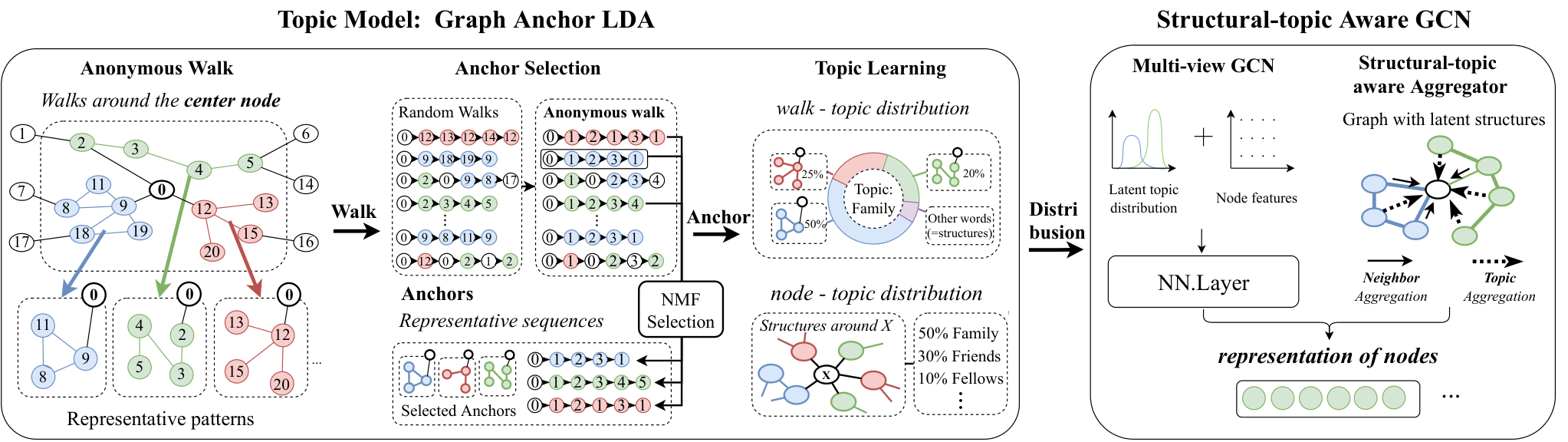
In response to these challenges, in this paper we propose Graph Structural Topic Neural Network, abbreviated GraphSTONE, a GCN framework featuring topic modeling of graph structures. Specifically, we model structural topics via anonymous walks (Micali and Zhu 2016) and Graph Anchor LDA. On one hand, anonymous walks are a flexible and efficient metric of depicting structural patterns, which only involve sampling instead of matching. On the other hand, we propose Graph Anchor LDA, a novel topic modeling algorithm that pre-selects “anchors”, i.e. representative structural patterns, which will be emphasized during the topic modeling. By doing so, we are relieved of the overwhelming volume of structural patterns and can thus focus on relatively few key structures. As a result, concise structural topics can be generated with better efficiency.
We also design multi-view graph convolutions that are able to aggregate node features and structural topic features simultaneously, and utilize the extracted structural topics to guide the aggregation. Extensive experiments are carried out on multiple datasets, where our model outperforms competitive baselines. In addition, we carry out visualization on a synthetic dataset, which provides intuitive understandings of both Graph Anchor LDA and GraphSTONE.
To summarize, we make the following contributions.
- (1)
We propose structural topic modeling on graphs that capture distributional differences over local structural patterns on graphs, which to the best of our knowledge, is the first attempt to utilize topic modeling on graphs.
- (2)
We enable topic modeling on graphs through anonymous walks and a novel Graph Anchor LDA algorithm, which are both flexible and efficient.
- (3)
We propose a multi-view GCN unifying both node features with structural topic features, which we show are complementary to each other.
- (4)
We carry out extensive experiments on multiple datasets, where GraphSTONE shows competence in both performance and efficiency.
2. Related Work
2.1. Graph Neural Networks (GNNs)
Recent years have witnessed numerous works focusing on deep architectures over graphs (Kipf and Welling 2017; Hamilton et al. 2017), among which the GCNs received the most attention. GCNs are generally based on neighborhood aggregation, where the computation of a node is carried out by sampling and aggregating features of neighboring nodes.
Although neighborhood aggregation makes GCNs as powerful as the Weisfeiler-Lehman (WL) isomorphism test (Xu et al. 2018; Morris et al. 2019; Li et al. 2019), common neighborhood aggregations refer to node features only, leaving them less capable in capturing complex neighborhood structures. Such weakness is also shown in theory. For example, (Loukas 2020) states that GCNs should be sufficiently wide and deep to be able to detect a given subgraph, while (Oono and Suzuki 2020) demonstrates that deep GCNs can learn little other than degrees and connected components.
To complement, many works have focused on GCNs with emphasis on higher-order local structural patterns. For example, (Lee et al. 2019) selects indicative motifs within a neighborhood before applying attention, which we claim to be insufficient. On the contrary, our work focuses on distributions over structures rather than individual structures. (Jin et al. 2020) captures local structural patterns via anonymous walks, which can capture complex structures yet suffers from poor efficiency. By comparison, our solution using topic models would be more efficient in that we pre-select anchors for topic modeling.
2.2. Modeling Graph Structures
There are many previous works on depicting graph structure properties using metrics such as graphlets and shortest paths (Shervashidze et al. 2009; Borgwardt and Kriegel 2005). However, they commonly require pattern matching, which is hardly affordable in large, real-world networks. In addition, these models are constrained to extract pre-designed structural patterns, which are not flexible enough to depict real-world networks with different properties. A parallel line of works, such as (Koutra et al. 2014) aim to decompose a graph into indicative structures. However, they focus on graph-level summarization but fail to generate node-level structural depictions.
Several works in network embedding also exploit network structures to generate node representations, such as (Ribeiro et al. 2017; Donnat et al. 2018; Long et al. 2019). However, their focuses are generally singular in that they do not refer to node features, while our model is able to combine both graph structures and node features through GCNs.
2.3. Topic Modeling
Topic modeling in NLP is a widely used technique aiming to cluster texts. Such models assign a distribution of topics to each document, and a distribution of words to each topic to provide low-dimensional, probabilistic descriptions of documents and words.
Latent Dirichlet Allocation (LDA) (Blei et al. 2003), a three-level generative model, embodies the most typical topic models. However, although prevalent in NLP (Liu et al. 2015; Kawamae 2019), LDA has hardly, if ever, been utilized in non-i.i.d. data like networks. In this work, we design a topic model on networks, where structural topics are introduced to capture distributional differences over structural patterns in networks.
3. Model: GraphSTONE
In this section we introduce our model Graph Structural-topic Neural Network, i.e. GraphSTONE. We first present the topic modeling on graphs, before presenting the multi-view graph convolution.
Fig. 2 gives an overview of our model GraphSTONE. Anonymous random walks are sampled for each node to depict local structures of a node. Graph Anchor LDA is then carried out on anonymous walks for each node, where we first select “anchors”, i.e. indicative anonymous walks through non-negative matrix factorization. After obtaining the walk-topic and node-topic distributions, we combine these structural properties with original node features through a multi-view GCN which outputs representations for each node.
3.1. Topic Modeling for Graphs
3.1.1. Anonymous Walks
We briefly introduce anonymous walks here and refer readers to (Micali and Zhu 2016; Ivanov and Burnaev 2018) for further details.
An anonymous walk is similar to a random walk, but with the exact identities of nodes removed. A node in an anonymous walk is represented by the first position where it appears. Fig. 2 (a) provides intuitive explanations of anonymous walks which we find appealing. For example, is a random walk starting from node 0, and its anonymous walk is defined as . It is highly likely that it is generated through a triadic closure.
We present the following theorem to demonstrate the property of anonymous walks in depicting graph structures.
Theorem 1.
(Micali and Zhu 2016) Let be the subgraph induced by all nodes such that and be the distribution of anonymous walks of length starting from , one can reconstruct using , where , is the number of edges in .
Theorem 1 underscores the ability of anonymous walks in describing local structures of nodes in a general manner. Therefore, we take each anonymous walk as a basic pattern for describing graph structures33 3 Although we do not explicitly reconstruct , such theorem demonstrates the ability of anonymous walks to represent structural properties..
3.1.2. Problem Formulation
We formulate topic modeling on graphs in our paper as follows.
Definition 1 (Topic Modeling on Graphs).
Given a graph , a set of possible anonymous walks of length as , and the number of desired structural topics , a topic model on graphs aims to learn the following parameters.
- •
A node-topic matrix , where a row corresponds to a distribution with denoting the probability of node belonging to the -th structural topic.
- •
A walk-topic matrix where a row is a distribution over and denotes the probability of belonging to the -th structural topic.
In addition, we define the set of anonymous walks starting from as , with as the number of walks to sample.
The formulation is an analogy to topic modeling in NLP, where anonymous walks correspond to words, and the sets of walks starting from each node correspond to documents. By making the analogy, nodes are given probabilistic depictions over their local structural patterns, and structural topics would thus consist of structural pattern distributions that are indicative towards node properties (social relations in Fig. 1, for example).
According to LDA constraints in NLP (Arora et al. 2012), we introduce Lemma 1 to show that the topic model in networks can indeed be learned.
Lemma 1.
There is a polynomial-time algorithm that fits a topic model on a graph with error , if and the length of walks satisfy
where is the number of topics, is the number of nodes. and are parameters related to topic imbalance defined in (Blei et al. 2003), which we assume to be fixed.
We first introduce the general idea of the lemma. In topic models in NLP, it is assumed that the length of each document as well as the vocabulary is fixed, while the corpus is variable-sized. Marked differences exist in graphs, where the number of nodes is fixed, while anonymous walk sets and samples are variable-sized. Hence we focus on instead of .
Proof.
(Arora et al. 2012) gives a lower bound on the number of documents such that the topic model can be fit, namely
where is the vocabulary size. As the latter term is constant, we focus on the first term.
We then get the bound of and , namely
The number of anonymous walks increases exponentially with length of walks (Ivanov and Burnaev 2018), i.e.,
Consequently we reach Lemma 1. ∎
3.1.3. Graph Anchor LDA
A large number of different walk sequences will be generated on complex networks, among which many may not be indicative, as illustrated in (Milo et al. 2002). If sequences are regarded separately, we would be encountered with a huge “vocabulary”, which would compromise our model, since the model may overfit on meaningless sequences and ignore more important ones.
Unfortunately, while in NLP the concept of stopwords is utilized to remove meaningless words, no such results exist in networks to remove such walk sequences. Consequently, we propose to select highly indicative structures first, which we call “anchors”, before moving on to further topic modeling.
Specifically, we define the walk-walk co-occurrence matrix , with , and adopt non-negative matrix factorization (NMF) (Lee and Seung 1999) to extract anchors
| (1) | ||||
We iteratively update until convergence, before finding the anchors by , where is the set of indices for anchors, and is the -th row of . Intuitively, by choosing the walks with largest weights, we are choosing the walks most capable of interpreting the occurrence of other walks, i.e. indicative walks. We later show theoretically that the selected walks are not only indicative of walk co-occurrences but also the underlying topics.
Based on the anchors we picked, we move forward to learn the walk-topic distribution . (Arora et al. 2013) presents a fast optimization for LDA with anchors as primary indicators and non-anchors providing auxiliary information. We get through optimizing
| (2) |
where is the re-arranged walk co-occurrence matrix with anchors lying in the first rows and columns, and is the row of for the -th anchor.
In addition, we define node-walk matrix as with denoting the occurrences of in . We then get the node-topic distribution through , where denotes pseudo-inverse.
3.1.4. Theoretical Analysis
We here provide a brief theoretical analysis of our Graph Anchor LDA in its ability to recover “anchors” of not only walk co-occurrences but also topics. We first formalize the notion of “anchors” via the definition of separable matrices.
Definition 2 (-separable matrices).
(Arora et al. 2012) An non-negative matrix is -separable if for each there is some row of that has a single nonzero entry with .
Specifically, if a walk-topic matrix is separable, we call the walks with non-zero weights “anchors”. We then present a corollary derived from (Arora et al. 2012) indicating that the non-negative matrix factorization is indeed capable of finding such anchors.
Corollary 0.
Suppose the real walk-node matrix (i.e. the real walk distribution of each node) is generated via , where is the real walk-topic matrix and is a matrix of coefficients, both non-negative. We define and as an observation of . For every , there is a polynomial time algorithm that factorizes such that . Moreover, if is -separable, then the rows of almost reconstruct the anchors up to an error of .
Specifically, the walk co-occurrence matrix serves as an estimate of the walk covariance in Corollary 2. Corollary 2 emphasizes that our Graph Anchor LDA algorithm is indeed able to select representative structural patterns within each structural topic. In reality, the topics are generally non-separable, where we will empirically show the effectiveness of anchor selection.
3.1.5. Discussion
We discuss the difference between Graph Anchor LDA and community detection, both of which can be used for dimensionality reduction on graphs. While community detection focuses on dense connections, Graph Anchor LDA focuses on the distribution of local structures, which will assign similar topics to structurally similar, but not necessarily connected nodes (e.g. and in Fig. 3). We will show such a difference by comparing Graph Anchor LDA with MNMF (Jin et al. 2019) in the experiments.
3.2. Structural-topic Aware GCN
We then introduce our design of graph convolutions which fuses structural topic features along with node features.
3.2.1. Structural-topic Aware Aggregator
Prevalent GCNs gather all neighbors with equal contributions, while GAT, although assigning different weights on neighbors, takes only node features but not structural properties into account. Consequently, we propose to utilize the learned structural topics to guide the aggregation of neighbors. We utilize the scheme of importance sampling for nodes based on the similarities of their structural topics, such that the neighborhood can be aggregated in a way that illustrates homophily, i.e. similar nodes influence each other more,
| (3) |
where denotes the output vector for node from the -th layer. We take identical as GraphSAGE while being flexible to more sophisticated methods.
3.2.2. Multi-view GCN
As the two types of features come from different domains, utilizing one to complement the other would be ideal. Inspired by the idea of boosting, we introduce two parallel GCNs, one focusing on structural topics and the other on node features correspondingly. Specifically, let and denote the outputs of the two GCNs for node at layer , we apply a nonlinear neural network layer on the two output vectors.
| (4) |
where is the final output of the multi-view GCN for node , and can be arbitrary operations, where we take as concatenation.
For the initialization of , we take , the node feature of , and be the concatenation of the following: a) the vector indicating the distribution of anchors in the neighborhood of , and b) the node-topic distribution .
Finally, we adopt the unsupervised objective of GraphSAGE (Hamilton et al. 2017) for learning the output vectors.
| (5) |
where is the sigmoid function, co-occurs with in random walks, and is the noise distribution for negative sampling.
We show the pseudo-code of GraphSTONE in Algorithm 1.
4. Experiments
In this section, we introduce our empirical evaluations of the model GraphSTONE. We first introduce experimental settings, before results on various tasks. Specifically, our evaluation consists of:
- •
Quantitative evaluation, including link reconstruction and node classification.
- •
Qualitative evaluation, including visualization tasks that illustrate the results of Graph Anchor LDA and GraphSTONE in a straightforward manner.
- •
Self evaluation, including analysis on model parameters and model components.
4.1. Experimental Setup
We first introduce the datasets, comparison methods as well as settings for experimental evaluation.
Datasets We utilize citation networks (Cora, Pubmed (Kipf and Welling 2017)), social network (Aminer (Zhang et al. 2019)) and protein interaction network (PPI) to evaluate our model. Dataset statistics are listed in Table 1.
| Datasets | Type | # Classes | ||
|---|---|---|---|---|
| Cora | Citation | 2,708 | 5,429 | 7 |
| AMiner | Social | 3,121 | 7,219 | 4 |
| Pubmed | Citation | 19,717 | 44,338 | 3 |
| PPI | Protein | 14,755 | 228,431 | 121 |
Baselines We take the following novel approaches in network representation learning as baselines.
- •
Structure models, focusing on structural properties of nodes. Here we choose a popular model Struc2Vec (Ribeiro et al. 2017).
- •
GNNs, including GraphSAGE, GCN (Kipf and Welling 2017) and GAT (Veličković et al. 2017). We train these models using the unsupervised loss of Eq. 5.
- •
GraphSTONE (nf). We take the outputs of Graph Anchor LDA directly as inputs of GCN to verify how the extracted structural topics on networks contribute to better GCN modeling. We denote this variant as GraphSTONE (nf). Note that GraphSTONE (nf) does not take raw node features as inputs.
Settings We take 64-dimensional embeddings for all methods, and adopt Adam optimizer with a learning rate of 0.005. For GNNs, we take 2-layer networks with a hidden layer sized 100. For skip-gram optimization (Eq. 5), we take , window size as 5 and the number of negative sampling . For models involving neighborhood sampling, we take the number for sampling as 20. We leave the parameters of other baselines as default mentioned in corresponding papers. In addition, we take for GraphSTONE.
We also introduce two settings for node classification tasks.
- •
Transductive. We allow all models access to the whole graph, i.e. all edges and node features. We apply this setting for Cora, AMiner, Pubmed and PPI.
- •
Inductive. The test nodes are unobserved during training. We apply this setting on PPI, where we train all GNNs on 20 graphs and directly predict on two fixed test graphs, as in (Hamilton et al. 2017). Note that only GNNs are capable of inductive classification.
Input Model Cora AMiner Pubmed AUC Recall@0.5 AUC Recall@0.5 AUC Recall@0.5 No features Struc2Vec 54.29 54.38 47.55 47.63 53.14 53.14 GraLSP 66.28 66.38 65.40 65.50 57.62 57.63 GCN 74.60 74.71 71.98 72.07 59.20 59.22 GraphSTONE (nf) 92.44 92.56 89.87 89.91 87.47 87.48 Features GCN 94.14 94.26 94.47 94.55 92.23 92.25 GAT 94.66 94.78 95.24 95.34 92.36 92.38 GraLSP 94.39 94.51 94.85 94.89 90.83 90.84 GraphSAGE 95.30 95.42 94.92 95.02 91.52 91.54 GraphSTONE 96.37 96.70 95.94 96.06 94.25 94.27
Input Model Cora AMiner Pubmed PPI Macro-f1 Micro-f1 Macro-f1 Micro-f1 Macro-f1 Micro-f1 Macro-f1 Micro-f1 30% 70% 30% 70% 30% 70% 30% 70% 30% 70% 30% 70% 30% 70% 30% 70% No features Struc2Vec 17.55 18.92 29.07 31.34 23.17 21.80 36.11 38.44 31.29 31.31 41.50 41.49 12.89 13.53 40.49 40.74 GraLSP 58.86 61.62 60.88 62.45 43.19 43.03 45.85 45.92 38.89 38.84 45.88 46.01 10.19 10.72 37.65 37.88 GCN 11.65 11.94 32.30 32.83 14.86 16.81 41.24 42.51 35.07 36.51 46.56 47.83 8.75 9.08 36.70 37.46 GraphSTONE (nf) 70.25 71.33 71.73 72.42 57.11 56.70 58.21 58.91 56.87 58.88 60.47 60.69 10.28 11.20 38.93 38.96 Features GCN 79.84 81.09 80.97 81.94 65.02 67.33 64.89 66.72 76.93 77.21 76.42 77.49 12.57 12.62 40.40 40.44 GAT 79.33 82.08 80.41 83.43 68.76 69.10 67.92 68.16 76.94 76.92 77.64 77.82 11.91 11.97 39.92 40.10 GraLSP 82.43 83.27 83.67 84.31 68.82 70.15 69.12 69.73 81.21 81.38 81.43 81.52 11.34 11.89 39.55 39.80 GraphSAGE 80.52 81.90 82.13 83.17 67.40 68.32 66.59 67.54 76.61 77.24 77.36 77.84 11.81 12.41 39.80 40.08 GraphSTONE 82.78 83.54 83.88 84.73 69.37 71.16 69.51 69.93 78.61 78.87 79.53 81.03 15.55 15.91 43.60 43.64
4.2. Proof-of-concept Visualization
As we propose a new problem – topic modeling on graphs, we first show a visualization result to intuitively explain its results. We carry out visualization on a synthetic dataset as a simple proof-of-concept. We design using three types of structures: one dense cluster, one T-shaped and one star, and then connect such structures interleavingly on a ring. We show an illustration of in Fig. 4(a). For a clear illustration, we replace each structure with a colored dot. Apparently, the nodes in possess three distinct structural properties (with the ring excluded), which can be regarded as three structural topics. We then obtain representation vectors from GraphSTONE, GraLSP and MNMF, and plot them on a 2d plane. We also obtain a node-topic distribution with using Graph Anchor LDA and also plot them on the plane.
As shown in Fig. 4(b) and 4(c), both Graph Anchor LDA and GraphSTONE cluster the three types of nodes clearly. The results are even more astonishing as GraLSP (Fig. 4(d)) fails to cluster nodes in a satisfactory manner, which shows that probabilistic topic modeling better captures indicative structural patterns and marks the difference between neighborhoods of nodes. Also, MNMF, a community-aware embedding algorithm, largely ignores the structural similarity between nodes and fails to separate nodes clearly.
Moreover, we visualize the walk-topic distributions generated by Graph Anchor LDA in Fig. 5(a), and compare them with those by ordinary LDA, where x-axis denotes indices of anonymous walks, and y-axis denotes the corresponding probability. It can be shown that the anchors selected by our Graph Anchor LDA are not only indicative of “topics”, but are also in accordance with the actual graph structures. Moreover, the walk-topic distributions generated by Graph Anchor LDA are indeed sharper than those by ordinary LDA, underscoring the need for selecting anchors. We hence conclude that Graph Anchor LDA is highly selective and interpretable in summarizing graph structures.
4.3. Quantitative Evaluations
We conduct experiments on link reconstruction and node classification to evaluate GraphSTONE quantitatively.
4.3.1. Link Reconstruction
We conduct link reconstruction using Cora, AMiner, and Pubmed, but not PPI as it contains disjoint graphs. We sample a proportion of edges from the initial network, which are used as positive samples, along with an identical number of random negative edges. It should be noted that the positive edges are not removed from training. We take the inner product of embedding vectors as the score for each sample, which is used for ranking. Samples with scores among top 50% are predicted as “positive” edges. We report AUC and Recall as metrics.
The results are shown in Table 2. It can be showed that by combining structural features with original node features, our model is able to generate representations that more accurately summarizes the original network. It is even more remarkable that based on structural features alone, GraphSTONE(nf) is able to significantly outperform the counterparts without the help of raw node features. Although Struc2Vec considers global network structures, its poor performance in link reconstruction reveals its shortage in capturing the simplest structure – edges. By comparison, GraphSTONE and GraphSTONE (nf) achieve a more elaborate balance among simple structures, like edges, and complex structures.
4.3.2. Node Classification
We then carry out node classification according to the setting of each dataset. For the transductive setting, different fractions of nodes are sampled randomly for testing, leaving the rest for training. For the inductive setting, we take embedding vectors of nodes from the training graphs for training, and those from the test graphs for testing. We use Logistic Regression as the classifier and take the macro and micro F1 scores for evaluation. The results are averaged over 10 independent runs.
Transductive classification Results of transductive node classification are shown in Table 3. It is generally shown that compared to competitive baselines, GraphSTONE is able to achieve satisfactory results. In addition, GraphSTONE (nf) significantly outperforms GCN without feature input, hence verifying that the structural topic information extracted by topic modeling does contribute significantly to more accurate representations of nodes.
Inductive classification Results of inductive classification are shown in Table 4. Note that algorithms that do not refer to node features are not inductive and thus not listed. It is shown that GraphSTONE also outperforms competitive GNNs, showing that the learned structural topic features generalize well across networks of the same type.
| Model | Macro-f1 | Micro-f1 |
|---|---|---|
| GCN | 12.15 | 40.85 |
| GAT | 12.31 | 39.76 |
| GraLSP | 12.59 | 40.81 |
| GraphSAGE | 11.92 | 40.05 |
| GraphSTONE | 18.14 | 46.02 |
4.4. Model Analysis
We carry out model analysis, including ablation studies, parameter analysis and efficiency. We use node classification to reflect the performance of the model.
4.4.1. Ablation studies
We carry out thorough ablation studies on the two parts of GraphSTONE, topic modeling and GCN and show the results in Table 5.
First, we delve deeper into the design of our Graph Anchor LDA by comparing it with several variants. On one hand, we vary the analogy of “words” by substituting anonymous walks with three other units of structures: individual nodes, distribution of node degrees in and random walks without anonymity. We denote the three variants as GraphSTONE (node), GraphSTONE (degree) and GraphSTONE (rw). On the other hand, we verify the contribution of “anchors” by comparing with GraphSTONE without anchors, referred to as GraphSTONE (no anchors). It can be shown that all three variants, GraphSTONE (node), (degree) and (rw) all fail to outperform GraphSTONE, probably because individual nodes and degrees only depict one-hop structures, and raw random walks are too sparse to observe co-appearance. By comparison, GraphSTONE (no anchors) performs better than the previous three due to its use of anonymous walks, but worse than GraphSTONE, which endorses the contribution of anchors in topic modeling and corresponds with Fig. 5(a).
| Model | Macro-f1 | Micro-f1 |
|---|---|---|
| GCN | 81.46 | 82.61 |
| GraphSTONE (node) | 82.33 | 83.55 |
| GraphSTONE (degree) | 81.29 | 82.36 |
| GraphSTONE (rw) | 82.35 | 82.85 |
| GraphSTONE (no anchors) | 83.12 | 83.39 |
| GCN-concat | 81.43 | 82.62 |
| GraphSTONE | 84.21 | 85.13 |


In addition, we validate the effectiveness of our structural multi-view GCN by comparing GraphSTONE with GCN-concat, a GCN with its input node features concatenated with structural topic features. It can be shown that with our designs of multi-view graph convolution, GraphSTONE enables node and structural features to complement each other, while simple aggregation fails to do so.
4.4.2. Parameter Analysis
We analyze two parameters in our model, the length of walks and the number of topics and plot the performances in Fig. 6. As shown, performances peak at certain choices for both parameters, while unduly set values, either too big or too small, will compromise the model performance. In addition, the sensitivity to parameter depends on whether to use node features. If node features are not used, GraphSTONE (nf) relies solely on structural topic features, thus being more sensitive to . By comparison, GraphSTONE is less sensitive to .
4.4.3. Efficiency
We compared the efficiency of GraphSTONE with several baselines: Struc2Vec, GCN and GraLSP. We train all models and report the time needed for convergence on a single machine equipped with a GPU with 12GB RAM.
Results are presented in Fig.7. It can be shown that GraLSP suffers from poor efficiency due to its direct modeling of anonymous walks. By comparison, GraphSTONE takes significantly less time than GraLSP, showing the effectiveness of topic modeling. In addition, GraphSTONE becomes even more efficient when anchors are extracted and barely takes more time than GCN.
4.5. Visualization
We carry out visualization on real-world datasets to qualitatively evaluate our model. We learn the representation vectors on Cora, which are then reduced to 2d vectors using PCA. We select representative models: Struc2Vec (structure models), GraphSAGE (GNNs) and GraLSP (structure GNNs), and our model to compare.
The results are shown in Fig.8, where different colors correspond to 7 labels in Cora. It is observed that GraphSTONE clusters nodes in a compact and separable manner, especially on certain colors (yellow, green and blue), compared with other methods.
5. Conclusion
In this paper, we present a GCN framework that captures local structural patterns for graph convolution, called GraphSTONE. To the best of our knowledge, it is the first attempt on topic modeling on graphs and GCNs. Specifically, we observe that the distributions, rather than individuals of local structural patterns are indicative towards node properties in networks, while current GCNs are scarcely capable of modeling. We then utilize topic modeling, specifically Graph Anchor LDA to capture the distributional differences over local structural patterns, and multi-view GCNs to incorporate such properties. We demonstrate that GraphSTONE is competitive, efficient and interpretable through multiple experiments.
For future work, we seek to extend our work to see how GNNs are theoretically improved by incorporating various graph structures.
Acknowledgements.
We are grateful to Ziyao Li for his insightful advice towards this work. This work was supported by the National Natural Science Foundation of China (Grant No. 61876006 and No. 61572041).References
- (1)
- Arora et al. (2013) Sanjeev Arora, Rong Ge, Yonatan Halpern, David Mimno, Ankur Moitra, David Sontag, Yichen Wu, and Michael Zhu. 2013. A practical algorithm for topic modeling with provable guarantees. In International Conference on Machine Learning. 280–288.
- Arora et al. (2012) Sanjeev Arora, Rong Ge, and Ankur Moitra. 2012. Learning topic models–going beyond SVD. In 2012 IEEE 53rd Annual Symposium on Foundations of Computer Science. IEEE, 1–10.
- Blei et al. (2003) David M Blei, Andrew Y Ng, and Michael I Jordan. 2003. Latent dirichlet allocation. Journal of machine Learning research 3, Jan (2003), 993–1022.
- Borgwardt and Kriegel (2005) Karsten M Borgwardt and Hans-Peter Kriegel. 2005. Shortest-path kernels on graphs. In Fifth IEEE international conference on data mining. IEEE, 8–pp.
- Donnat et al. (2018) Claire Donnat, Marinka Zitnik, David Hallac, and Jure Leskovec. 2018. Learning structural node embeddings via diffusion wavelets. In Proceedings of the 24th ACM SIGKDD International Conference on Knowledge Discovery & Data Mining. 1320–1329.
- Granovetter (1977) Mark S Granovetter. 1977. The strength of weak ties. In Social networks. Elsevier, 347–367.
- Hamilton et al. (2017) Will Hamilton, Zhitao Ying, and Jure Leskovec. 2017. Inductive representation learning on large graphs. In Advances in Neural Information Processing Systems. 1024–1034.
- Ivanov and Burnaev (2018) Sergey Ivanov and Evgeny Burnaev. 2018. Anonymous Walk Embeddings. In International Conference on Machine Learning. 2191–2200.
- Jin et al. (2019) Di Jin, Xinxin You, Weihao Li, Dongxiao He, Peng Cui, Françoise Fogelman-Soulié, and Tanmoy Chakraborty. 2019. Incorporating network embedding into markov random field for better community detection. In Proceedings of the AAAI Conference on Artificial Intelligence, Vol. 33. 160–167.
- Jin et al. (2020) Yilun Jin, Guojie Song, and Chuan Shi. 2020. GraLSP: Graph Neural Networks with Local Structural Patterns. In The Thirty-Fourth AAAI Conference on Artificial Intelligence, AAAI 2020, New York, NY, USA. AAAI Press, 4361–4368.
- Kawamae (2019) Noriaki Kawamae. 2019. Topic Structure-Aware Neural Language Model: Unified language model that maintains word and topic ordering by their embedded representations. In The World Wide Web Conference. ACM, 2900–2906.
- Kipf and Welling (2017) Thomas Kipf and Max Welling. 2017. Semi-Supervised Classification with Graph Convolutional Networks. In International Conference of Learning Representations.
- Koutra et al. (2014) Danai Koutra, U Kang, Jilles Vreeken, and Christos Faloutsos. 2014. Vog: Summarizing and understanding large graphs. In Proceedings of the 2014 SIAM international conference on data mining. SIAM, 91–99.
- Lee and Seung (1999) Daniel D Lee and H Sebastian Seung. 1999. Learning the parts of objects by non-negative matrix factorization. Nature 401, 6755 (1999), 788.
- Lee et al. (2019) John Boaz Lee, Ryan A Rossi, Xiangnan Kong, Sungchul Kim, Eunyee Koh, and Anup Rao. 2019. Graph Convolutional Networks with Motif-based Attention. In Proceedings of the 28th ACM International Conference on Information and Knowledge Management. 499–508.
- Li et al. (2019) Ziyao Li, Liang Zhang, and Guojie Song. 2019. GCN-LASE: towards adequately incorporating link attributes in graph convolutional networks. In Proceedings of the 28th International Joint Conference on Artificial Intelligence. AAAI Press, 2959–2965.
- Liu et al. (2017) Lin Liu, Lin Tang, Libo He, Shaowen Yao, and Wei Zhou. 2017. Predicting protein function via multi-label supervised topic model on gene ontology. Biotechnology & Biotechnological Equipment 31, 3 (2017), 630–638.
- Liu et al. (2015) Yang Liu, Zhiyuan Liu, Tat-Seng Chua, and Maosong Sun. 2015. Topical word embeddings. In Twenty-Ninth AAAI Conference on Artificial Intelligence.
- Long et al. (2019) Qingqing Long, Yiming Wang, Lun Du, Guojie Song, Yilun Jin, and Wei Lin. 2019. Hierarchical Community Structure Preserving Network Embedding: A Subspace Approach. In Proceedings of the 28th ACM International Conference on Information and Knowledge Management. 409–418.
- Loukas (2020) Andreas Loukas. 2020. What graph neural networks cannot learn: depth vs width. In International Conference on Learning Representations. https://openreview.net/forum?id=B1l2bp4YwS
- Micali and Zhu (2016) Silvio Micali and Zeyuan Allen Zhu. 2016. Reconstructing markov processes from independent and anonymous experiments. Discrete Applied Mathematics 200 (2016), 108–122.
- Milo et al. (2002) Ron Milo, Shai Shen-Orr, Shalev Itzkovitz, Nadav Kashtan, Dmitri Chklovskii, and Uri Alon. 2002. Network motifs: simple building blocks of complex networks. Science 298, 5594 (2002), 824–827.
- Morris et al. (2019) Christopher Morris, Martin Ritzert, Matthias Fey, William L Hamilton, Jan Eric Lenssen, Gaurav Rattan, and Martin Grohe. 2019. Weisfeiler and leman go neural: Higher-order graph neural networks. In Proceedings of the AAAI Conference on Artificial Intelligence, Vol. 33. 4602–4609.
- Oono and Suzuki (2020) Kenta Oono and Taiji Suzuki. 2020. Graph Neural Networks Exponentially Lose Expressive Power for Node Classification. In International Conference on Learning Representations. https://openreview.net/forum?id=S1ldO2EFPr
- Ribeiro et al. (2017) Leonardo FR Ribeiro, Pedro HP Saverese, and Daniel R Figueiredo. 2017. struc2vec: Learning node representations from structural identity. In Proceedings of the 23rd ACM SIGKDD International Conference on Knowledge Discovery and Data Mining. ACM, 385–394.
- Shervashidze et al. (2009) Nino Shervashidze, SVN Vishwanathan, Tobias Petri, Kurt Mehlhorn, and Karsten Borgwardt. 2009. Efficient graphlet kernels for large graph comparison. In Artificial Intelligence and Statistics. 488–495.
- Veličković et al. (2017) Petar Veličković, Guillem Cucurull, Arantxa Casanova, Adriana Romero, Pietro Lio, and Yoshua Bengio. 2017. Graph attention networks. arXiv preprint arXiv:1710.10903 (2017).
- Xu et al. (2018) Keyulu Xu, Weihua Hu, Jure Leskovec, and Stefanie Jegelka. 2018. How powerful are graph neural networks? arXiv preprint arXiv:1810.00826 (2018).
- Zhang et al. (2019) Yizhou Zhang, Guojie Song, Lun Du, Shuwen Yang, and Yilun Jin. 2019. DANE: Domain Adaptive Network Embedding. In Proceedings of the Twenty-Eighth International Joint Conference on Artificial Intelligence.
- Zhou et al. (2018) Lekui Zhou, Yang Yang, Xiang Ren, Fei Wu, and Yueting Zhuang. 2018. Dynamic network embedding by modeling triadic closure process. In Thirty-Second AAAI Conference on Artificial Intelligence.