Ferroelectricity-induced multiorbital odd-frequency superconductivity in SrTiO3Preprint: APS/123-QED
Abstract
We demonstrate that SrTiO3 can be a platform for observing the bulk odd-frequency superconducting state owing to the multiorbital/multiband nature. We consider a three-orbital tight-binding model for SrTiO3 in the vicinity of a ferroelectric critical point. Assuming an intraorbital spin-singlet -wave superconducting order parameter, it is shown that the odd-frequency pair correlations are generated due to the intrinsic LS coupling which leads to the local orbital mixing. Furthermore, we show the existence of additional odd-frequency pair correlations in the ferroelectric phase, which is induced by an odd-parity orbital hybridization term proportional to the ferroelectric order parameter. We also perform a group theoretical classification of the odd-frequency pair amplitudes based on the fermionic and space group symmetries of the system. The classification table enables us to predict dominant components of the odd-frequency pair correlations based on the symmetry of the normal state Hamiltonian that we take into account. Furthermore, we show that experimental signatures of the odd-parity orbital hybridization, which is an essential ingredient for the ferroelectricity-induced odd-frequency pair correlations, can be observed in the spectral functions and density of states.
pacs
Valid PACS appear hereI Introduction
The Berezinskii rule Balatsky and Abrahams 1992 is a statement about the permutation anti-symmetry of the anomalous Green’s function under a simultaneous exchange of spin, coordinate, time, later extended to any orbital indices of the single-particle fermionic operators, for a summary see e.g. Linder and Balatsky 2019. The generalization allows for an extension of the possible symmetries of the superconducting order parameter to those that are both non-local and odd under the sign reversal of the relative time coordinate, or, equivalently, frequency. Originally proposed by Berezinskii Berezinskii 1974a; *Berezinskii74 as an odd-frequency spin-triplet -wave order parameter for superfluid 3He, it was soon considered as a possible candidate in various superconducting systems, including disordered systems Kirkpatrick and Belitz 1991, heavy fermion Coleman et al. 1993 and Kondo systems Coleman et al. 1994; Coleman et al. 1995; Fuseya et al. 2003. More recently, it was considered in the context of topological materials Huang et al. 2015; Gnezdilov 2019; Tanaka et al. 2011, such as Dirac semimetals Sukhachov et al. 2019, but a conclusive evidence for a thermodynamically stable odd-frequency superconducting order parameter is still lacking.
Notwithstanding the issue of thermodynamic stability, various exotic properties in bulk superconducting materials are associated with enhanced pair correlations in the odd-frequency channel. A very promising route in generating odd-frequency pair correlations is in multiband (multiorbital, multichannel) systems Black-Schaffer and Balatsky 2013; Triola et al. 2020, where, under fairly general conditions, such as band hybridization, odd-frequency interband pairing is generated even if the superconducting order parameter is strictly intraband and even-frequency. Candidates where such conditions are met were conceived in iron-pnictide superconductors Moreo et al. 2009; *Moreo2012; Youmans et al. 2018, systems with disorder Komendová et al. 2015, multi-channel Kondo systems Emery and Kivelson 1992; Cox and Zawadowski 1998, quantum spin Hall insulators on a honeycomb lattice Kuzmanovski and Black-Schaffer 2017, and driven systems Triola and Balatsky 2017. In the presence of spin-orbit coupling, such as the case of Sr2RuO4, it leads to Kerr effect Komendová and Black-Schaffer 2017; Triola and Black-Schaffer 2018.
SrTiO3 (STO) is an example of multiband (multiorbital) superconductors, and hence is an ideal candidate platform for observing the generation of odd-frequency pair correlations and associated features. The bands crossing the Fermi level are due to the three orbitals, whose degeneracy is further lifted by spin-orbit coupling and the tetragonal crystal field due to antiferrodistortive rotations. The issue of the numerous superconducting bands and gaps in STO is a subject of a debate. The existence of multiple superconducting gaps is indicated by early tunneling measurement Binnig et al. 1980, quantum oscillation measurement Lin et al. 2014a, and thermal conductivity data Lin et al. 2014b. These experimental data encouraged various theoretical studies about the multiband/multiorbital effects on the superconductivity in STO Fernandes et al. 2013; Edge and Balatsky 2015; Trevisan et al. 2018; Kanasugi and Yanase 2019. On the other hand, recent tunneling experiment Swartz et al. 2018 and optical conductivity data Thiemann et al. 2018 suggest single superconducting gap in STO.
Another intriguing feature of STO is the relationship between superconductivity and ferroelectric (FE) instability. The superconducting state in STO emerges in very low carrier density regime on the order of 1017 cm-3 Schooley et al. 1964; Lin et al. 2013; Lin et al. 2014a; Bretz-Sullivan et al. 2019, where the pairing mechanism cannot be captured by the Migdal-Eliashberg theory due to extreme retardation effects. Although various pairing interactions (e.g, plasmons Takada 1980; Ruhman and Lee 2016, localized longitudinal optical modes Gor’kov 2016; Gor’kov 2017) have been proposed to explain the persistence of superconductivity in the dilute density limit, the issue of the pairing mechanism has not yet been settled. On the other hand, STO is a quantum paraelectric (PE) in the vicinity of a FE quantum critical point Müller and Burkard 1979, and which can undergo a FE transition under various chemical and physical actions such as isovalent substitution of Sr with Ca Bednorz and Müller 1984, isotope substitution of oxygen Itoh et al. 1999, strain Uwe and Sakudo 1976, and electric field Hemberger et al. 1995. This FE instability motivated proposals of the pairing scenarios related to optical phonons mediating FE fluctuations Edge et al. 2015; Dunnett et al. 2018; Wölfle and Balatsky 2018; Arce-Gamboa and Guzmán-Verri 2018; Kedem 2018; van der Marel et al. 2019; Gastiasoro et al. 2020; Sumita and Yanase 2020. Indeed, enhancement of the superconducting transition temperature near a FE quantum critical point has been observed experimentally Stucky et al. 2016; Rischau et al. 2017; Tomioka et al. 2019; Ahadi et al. 2019; Herrera et al. 2019. Furthermore, the coexistent phase of superconducting and FE-like orders, so-called FE superconducting state Kanasugi and Yanase 2018; Kanasugi and Yanase 2019, was recently observed in experiments Rischau et al. 2017; Russell et al. 2019.
In this work, we consider a three-orbital tight-binding model of STO in the vicinity of a FE critical point. Superconductivity is assumed to be due to some intraorbital spin-singlet isotropic order parameter. Under a FE transition, an additional Rashba-like spin-orbit coupling term appears proportional to the spontaneous FE order parameter that decreases the point group symmetry of the material from to . We not only demonstrate that these ingredients guarantee the generation of odd-frequency pair correlations, but also classify them by combining the Berezinskii rule and the space group symmetry in the PE and FE phase of the system. The classification table indicates that some components, although allowed by symmetry, are not dynamically generated by the terms of the normal state Hamiltonian that we take into account. Furthermore, we show that signatures of the odd-parity orbital hybridization, which is essential for the ferroelectricity-induced odd-frequency pair correlations, can be observed in the spectral functions and density of states (DOS).
The rest of the article is organized as follows. In Sec. II, we demonstrate a group theoretical classification of the multiorbital odd-frequency pair amplitudes based on the Berezinskii rule and space group symmetry of the system. As a specific example, we provide a classification table of the odd-frequency pair amplitudes in electron systems such as STO. In Sec. III, a three-orbital tight-binding model of bulk STO near a FE critical point is introduced. By using this model, we study the odd-frequency pair amplitudes in Sec. IV. It is shown that some components of the even-parity odd-frequency pair amplitudes are generated by the intrinsic LS coupling in the PE phase. Furthermore, we show that a FE transition induces the generation of additional odd-parity odd-frequency pair amplitudes and the enhancement of even-parity odd-frequency pair amplitudes. It is confirmed that the symmetry of the odd-frequency pair amplitudes is consistent with the results of the group theoretical classification in Sec. III. In Sec. V, we show that experimental signatures of the ferroelectricity-induced odd-parity hybridization can be observed in the orbital-resolved spectral functions and double-peak structure of DOS. Finally, a brief summary and conclusion are given in Sec. VI.
II Symmetry of multiorbital odd-frequency pair correlations
II.1 Fermionic symmetry
We begin our discussion by classifying multiorbital superconducting states based on the fermionic symmetry, namely the Berezinskii rule Balatsky and Abrahams 1992; Black-Schaffer and Balatsky 2013. The pair amplitude, namely the anomalous Green’s function, can be defined in a multiorbital system as
| (1) |
where is the imaginary time and is the annihilation operator for an electron with momentum , orbital index , and spin . denotes the time-ordering operator for . The Matsubara representation of Eq. (1) is given by
| (2) |
where is a Matsubara frequency for the inverse temperature . We here consider the spacial, time, spin, and orbital parities of Cooper pairs in a multiorbital system. The spacial inversion operation is defined as
| (3) |
The time inversion operation , which changes sign of the relative time (not to be confused with the time reversal operation), acts on the Matsubara anomalous Green’s function as
| (4) |
The spin inversion operation and the orbital index inversion operation , simple swap operators permuting respective indices, are introduced as:
| (5) | |||||
| (6) |
The Fermi-Dirac statistics gives the sign change of the anomalous Green’s function under the combined action of the spacial, time, spin, and orbital index inversion operations as
| (7) |
which we write symbolically as . The full symmetries of the Cooper pair that satisfies Eq. (7) are summarized in Table 1.
| Pairing | |||||
|---|---|---|---|---|---|
Then, we perform the classification of the pair amplitude based on the results in Table 1. First of all, the anomalous Green’s function can be decomposed as
| (8) |
where is a identity matrix and are the Pauli matrices. We here used the abbreviate notation . The spin-singlet (triplet) pair amplitude () is even (odd) under the spin inversion . Furthermore, we define the orbital-singlet and orbital-triplet pair amplitudes as
| (9) | ||||
| (10) |
The orbital-triplet pair amplitudes and are even under the orbital index inversion . On the other hand, the orbital-singlet pair amplitudes and are odd under the orbital index inversion .
Using Eqs. (9) and (10), the odd-frequency pair amplitudes, that are odd under the time inversion , can be obtained as follows:
| (11) | ||||
| (12) | ||||
| (13) | ||||
| (14) |
where we suppressed the -dependence for brevity. The spin-triplet pair amplitudes are described by using a vector notation . The above odd-frequency pair amplitudes satisfy the Berezinskii rule (i.e., ).
II.2 Space group symmetry
In the previous section, we classified a multiorbital odd-frequency superconducting state based on the fermionic symmetry of the Cooper pair. Superconducting state can also lower point group symmetry of the state and any pairing state can be classified by the space group symmetry of the crystal structure Sigrist and Ueda 1991. Here, we provide a classification of multiorbital superconducting states based on the space group symmetry by considering the transformation of the Bloch wave function.
A creation operator of a Bloch state with orbital index and spin can be defined as
| (15) |
where represents the position for the unit cell (lattice vector). Using Eq. (15), the creation operator is transformed by a space group operation as follows:
| (16) | |||||
where and are the representation matrices for a point group operation in spin and orbital space, respectively. By defining , Eq. (16) is rewritten as
| (17) |
From Eq. (17), the pair amplitude is transformed by a space group operation as
| (18) | |||||
where the corresponding representation matrices are
| (19) | ||||
| (20) |
and is the representation matrix of the irreducible representation (IR) of the gap function. Note that the frequency dependence of the pair amplitude is not changed by the space group operations. By using Eq. (18), we can classify the -dependence of pair amplitudes under a given space group symmetry.
II.3 Application to polar electron systems
In this section, we perform the classification of the multiorbital odd-frequency pair amplitude based on both fermionic and space group symmetries. As far as we know, we here provide a first example of group theoretical classification for the multiorbital odd-frequency superconductivity, although that for the multiorbital even-frequency superconductivity Nomoto et al. 2016 and single-orbital odd-frequency superconductivity Geilhufe and Balatsky 2018 has been done in previous works. Note that we can classify the even-frequency pair amplitude in the same manner (see Appendix A).
As a demonstration, we here consider a time-reversal symmetric electron system in tetragonal or point group. To simplify the discussion, we assume -wave superconducting states which belong to trivial IR (i.e., ). Then, according to Eq. (18), it is sufficient to classify the pair amplitudes based on the point group symmetry, not space group symmetry. Extension to anisotropic superconducting states that transform in accordance with nontrivial IRs is straightforward. The basis functions for -dependence of the odd-frequency pair amplitudes, that are determined by using Eq. (18), are listed in Table 2. When the anomalous Green’s function belongs to the trivial IR of point group, that is IR, only the even-parity () pair amplitudes and in Table 2 are allowed. Then, the odd-parity () pair amplitudes should vanish because they do not belong to IR due to the sign change under spacial inversion operation . On the other hand, the odd-parity pair amplitudes may be trivial under all symmetry operations in point group, since point group can be decomposed as . Therefore, the odd-parity pair amplitudes and belonging to IR in point group are listed in Table 2, because is reduced to the trivial IR in point group. In the microscopic analysis of a three-orbital model (Secs. III and IV), we obtain pair amplitudes compatible with Table 2.
The odd-parity pair amplitudes are symmetrically forbidden in centrosymmetric point group, when the superconductivity belongs to the trivial IR as expected in STO. In order to induce the odd-parity pair amplitudes, a spacial inversion symmetry breaking, which descends the crystallographic point group from to , is necessary. This symmetry lowering from to can be realized by a FE phase transition, such as a polar inversion symmetry breaking that actually occurs in STO Bednorz and Müller 1984; Itoh et al. 1999; Uwe and Sakudo 1976; Hemberger et al. 1995.
| -dependence of | IR | |
| -dependence of | IR | |
| -dependence of | IR | |
| -dependence of | IR | |
III Model and method
In this section, we introduce an electron-lattice coupled multiorbital model for bulk STO.
III.1 Three-orbital model
First, we introduce a three-orbital tight-binding model for electrons in bulk STO as follows:
| (21) | ||||
| (22) | ||||
| (23) | ||||
| (24) | ||||
| (25) |
where orbitals are denoted by the orbital index , respectively. The tight-binding forms are given by
| (26) | |||||
| (27) | |||||
| (28) | |||||
| (29) |
The first term is the kinetic-energy term of orbitals. The single electron kinetic energy includes the chemical potential and the tetragonal crystal field arising from the antiferrodistortive structural transition. The chemical potential is determined to fix the carrier density per Ti site as . The second term represents the atomic LS coupling of Ti ions. The orbital angular momentum operator is defined as
| (30) |
in the orbital basis . Here, is the projection of the angular momentum operator onto the orbital subspace. The band structure of bulk STO is reproduced by with the parameter set Hirayama et al. 2012; Khalsa and MacDonald 2012; Zhong et al. 2013; Kanasugi and Yanase 2019, where the unit of energy is chosen as . The third term is an intersite odd-parity orbital hybridization term. Since belongs to IR of point group, it is allowed only in the FE phase with broken mirror symmetry along the axis. Then, the hopping integral can be treated as a FE order parameter which characterize the polar inversion symmetry breaking along the [001] axis Kanasugi and Yanase 2019 (i.e., ). Combination of and leads to the Rashba-type spin-orbit splitting of the band structure in the FE phase. We study superconductivity by adopting the BCS-type static attractive interaction . For simplicity, we assume momentum-independent intraorbital pairing interaction. is the number of Ti sites, and is the pairing interaction strength.
In this study, we apply the mean-field approximation to as
| (31) |
by introducing the orbital-dependent superconducting order parameter,
| (32) |
Note that under 4-fold rotational symmetry. By introducing the multiorbital Nambu spinors
| (33) | ||||
| (34) |
we obtain the matrix representation of the mean-field Hamiltonian as
| (35) |
The Bogoliubov-de Gennes (BdG) Hamiltonian is described as
| (36) |
where the normal state part and pairing part are given by
| (37) |
The BdG Hamiltonian is diagonalized by carrying out the Bogoliubov transformation as
| (38) |
where is the annihilation operator for a Bogoliubov quasiparticle with momentum , pseudoorbital , and pseudospin . Then, Eq. (35) is rewritten as
| (39) | |||||
and hence the electronic free energy per Ti site is obtained as
| (40) | |||||
Here, we used an abbreviate notation . The last term of Eq. (40) is necessary since the carrier density per Ti site is fixed as instead of fixing the chemical potential . Using obtained by solving Eq. (32), we calculate the electronic part of the free energy from Eq. (40).
III.2 Polar lattice distortion
Next, we introduce the Landau free energy arising from the polar lattice distortion as
| (41) |
where , , and are the lattice parameters which describe the elasticity of the lattice Kanasugi and Yanase 2019. The temperature dependence of lattice parameters is neglected in accordance with the fact that the dielectric constant in bulk STO is almost constant at low temperatures Müller and Burkard 1979.
Then, the total free energy including the contributions of both electrons and lattice is given by
| (42) |
The thermodynamically stable state is determined by minimizing the free energy with respect to and Kanasugi and Yanase 2018; Kanasugi and Yanase 2019. The values of and are determined to cut off the FE order parameter in a realistic regime Zhong et al. 2013; Kanasugi and Yanase 2019. The lattice parameter is a control parameter for the ferroelectricity, and we determined its value so as to realize a PE normal state near a FE critical point. Then, we consider the superconductivity in bulk STO which is tuned toward the vicinity of the FE critical point by isovalent substitution of Sr with Ca Bednorz and Müller 1984, isotope substitution of oxygen Itoh et al. 1999, strain Uwe and Sakudo 1976, electric field Hemberger et al. 1995, and by any other means.
III.3 Numerical setup
To study the interplay of odd-frequency superconductivity and FE transition in bulk STO, we perform numerical calculations in a dilute carrier density regime in which both the superconductivity and ferroelectricity can be stabilized simultaneously owing to the Lifshitz transition Kanasugi and Yanase 2019.
The carrier density is fixed as which corresponds to cm-3 by adopting the lattice constant of STO ( Å) as the unit of length. The pairing interaction is chosen to be which gives the superconducting transition temperature K at . The value of is set to be larger than the realistic transition temperature ( 0.3 K) to reduce the cost of the numerical calculation. The cutoff lattice parameters are chosen as . Then, the coexistent phase of superconductivity and ferroelectricity is stabilized when the lattice parameter is set to be smaller than a critical value. The value of and obtained results of the superconducting and FE order parameters at almost zero temperature () are summarized in Table 3.
| PE phase | FE phase | |
|---|---|---|
| 0 | 0.105 | |
| 0.00160 | 0.00277 | |
| 0.000268 | 0.00138 |
IV Odd-frequency pair correlations
On the basis of numerical solution of the electron-lattice coupled three-orbital model, we elucidate odd-frequency pair amplitudes in bulk STO. Using the BdG Hamiltonian matrix in Eq. (37), we obtain the full Matsubara Green’s function matrix as
| (43) |
where is a identity matrix. The matrix structure of is described as
| (44) |
The submatrix and are the normal and anomalous Green’s functions, respectively. () is the particle-hole counterpart of (). By applying Eqs. (11)-(14) to the matrix elements of , we calculate the odd-frequency pair amplitudes in bulk STO.
IV.1 Paraelectric phase
First, we consider the odd-frequency pairing in the PE phase with point group symmetry. Since we assumed the -wave () pairing [Eq. (25)], the odd-frequency pair amplitudes should belong to IR in the PE phase. Then, the even-parity odd-frequency pair amplitudes can be finite. The orbital hybridization due to the LS coupling [Eq. (23)] is essential for the odd-frequency Cooper pairs because they disappear in the absence of the LS coupling. The representative components of even-parity odd-frequency pair amplitudes at are shown in Fig. 1. Because of the time-reversal symmetry, the spin-singlet (spin-triplet) even-parity orbital-singlet (orbital-triplet) odd-frequency pair amplitude () is pure imaginary (real). The pair amplitude is normalized by a maximum value of the BCS pair amplitude which is defined as
| (45) |
where is given by Eq. (56) in Appendix A. As shown in Fig. 1(a), the spin-singlet even-parity orbital-singlet odd-frequency pair amplitude is not generated in our model although it is symmetrically allowed. On the other hand, some components of the spin-triplet even-parity orbital-triplet odd-frequency pair amplitudes , that have - or -wave like -dependence, are generated although their value is small compared to the BCS pair amplitude [Figs. 1(b) and 1(c)]. These results can be understood on the basis of the group theoretical classification in Sec.II.3. Table 2 shows that the -dependence of is proportional to ( and ) near the point. This means that the generation of requires the existence of terms proportional to in the model Hamiltonian. Indeed, the even-parity interorbital hybridizations proportional to are allowed by symmetry, and they may generate odd-frequency pair amplitudes . However, we omitted such hybridizations since their amplitude is tiny in bulk STO Hirayama et al. 2012; Khalsa and MacDonald 2012; Zhong et al. 2013; Kanasugi and Yanase 2019. Then, is not induced in our model. On the other hand, Table 2 also shows that -dependence of some components in are given by a linear combination of (e.g., ). Thus, the generation of these components is expected in bulk STO. We found finite , , and in the PE phase as expected. Intraorbital components vanish similarly to .
IV.2 Ferroelectric phase
Next, we investigate the odd-frequency pairing in the FE phase with point group symmetry. In the FE phase, the odd-parity odd-frequency pair amplitudes, that belong to IR, can also be induced owing to the breakdown of the spacial inversion symmetry. Figure 2 shows the -dependence of the representative components of odd-parity odd-frequency pair amplitudes. Owing to the time-reversal symmetry, the spin-singlet (spin-triplet) odd-parity orbital-triplet (orbital-singlet) odd-frequency pair amplitude () is real (pure imaginary). They have -wave like -dependence in consistent with the group theoretical classification in Table 2. These ferroelectricity-induced odd-frequency pair amplitudes originate from the odd-parity interorbital hybridization which appear in the FE phase [Eq. (24)], and hence they should have -wave like -dependence (e.g., -wave like pair amplitude is not driven by the FE order along the [001] axis, although it is allowed by symmetry). We confirmed that , , , , , and are induced by the FE transition in bulk STO [Fig. 2] in accordance with the group theoretical classification as well as above discussions. In addition, the odd-parity interorbital hybridization also generates some components of the even-parity odd-frequency pair amplitudes, whose -dependences are proportional to (). For instance, takes a finite value in the FE phase [Fig. 3(a)] although it is zero in the PE phase [Fig. 1(a)]. We found that , , , , , , , , and are finite in the FE phase [Fig. 3].
V Experimental signaures of odd-parity orbital hybridization
In this section, we demonstrate possible experimental signatures of the ferroelectricity-induced odd-parity orbital hybridization that leads to the emergence and enhancement of the odd-frequency pair amplitudes in bulk STO.
V.1 Spectral function
First, we study the spectral function which can be directly measured by the angle-resolved photoemission spectroscopy (ARPES). Using the Matsubara representation of the normal Green’s function in Eq. (44), the spectral function is obtained as
| (46) |
Here, we define the orbital-resolved spectral function as
| (47) |
whose -dependences are shown in Fig. 4. The electronic structure near the Fermi level is mainly constructed from and orbitals in the PE phase [Figs. 4(a) and 4(c)]. Then, and orbitals are responsible for the superconductivity, and the orbital-resolved spectral function clearly shows a single superconducting gap at zero energy. In the FE phase, the orbital-resolved spectral functions exhibit the Rashba spin-orbit splitting due to the spacial inversion symmetry breaking [Figs. 4(b) and 4(d)]. Since the odd-parity hybridization induces the mixing between and orbitals, the weight of orbital at the Fermi level is enhanced by the FE transition [compare Fig. 4(d) with Fig. 4(c)]. Thus, the contribution of orbital to the superconductivity is increased in the FE phase.
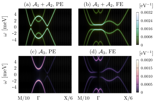
V.2 Density of states
To see the detail of the superconducting gap structure, we here investigate the DOS which can be measured by tunneling spectroscopy. The DOS is obtained by taking the trace of the spectral function as
| (48) |
where we defined the orbital-resolved DOS . Figure 5 shows the total and orbital-resolved DOS in bulk STO. Because of the 4-fold rotational symmetry of the system, the orbital-resolved DOS for orbital and that for orbital are equivalent.
In the PE phase, the DOS exhibits the BCS-like form with a single set of coherence peaks [Fig. 5(a)]. The coherence peaks originate from since the electronic states near the Fermi level are mainly constructed from orbitals [see Figs. 4(a) and 4(c)]. In the FE phase, the orbital-resolved DOS for orbital becomes comparable to owing to the odd-parity hybridization in the FE phase [Fig. 5(b)]. The total DOS shows two sets of the coherence peaks in the FE phase. The lower energy coherence peaks originate from both and , and hence they are generated by all of orbitals. On the other hand, the higher energy coherence peaks originate only from . We also note that the DOS shows the ferroelectricity-induced enhancement of superconducting gap which originates from the Lifshitz transition Kanasugi and Yanase 2019.
V.3 Gap functions in band basis
To clarify the ferroelectricity-induced splitting of coherence peaks in the DOS, we here investigate the superconducting gap functions in the band basis. We carry out the band diagonalization for the BdG Hamiltonian as follows:
| (49) |
where the unitary matrix is defined as
| (50) |
The unitary matrix diagonalizes the normal state part of the BdG Hamiltonian , and then the diagonal submatrix is obtained as
| (51) | ||||
| (52) |
Here, denotes the energy spectrum in the normal state [ () and ]. In the PE phase, the energy spectrum is 2-fold degenerate (i.e., ) owing to the spacial inversion and time-reversal symmetries. The pairing part of the BdG Hamiltonian in the band basis can be described as
| (53) | ||||
| (54) |
In our calculations, the superconductivity is dominated by the two lowest energy bands that construct the Fermi surfaces. Then, the effective two-band Hamiltonian for the two lowest energy bands can be obtained as
| (55) |
by neglecting the higher energy bands that do not give rise to the Fermi surface. Figure 6 shows the superconducting gap functions and 2-fold degenerate Fermi surfaces in the PE phase. It is shown that the pseudospin-singlet superconducting state is stabilized (i.e., [Figs. 6(a) and 6(b)] and ). Thus, the superconducting gap in the PE phase is given by , and its magnitude is consistent with the zero energy gap in the DOS [compare Fig. 5(a) with Fig. 6(c)]. On the other hand, Fig. 7 shows the superconducting gap functions and Rashba-split Fermi surfaces in the FE phase. It is shown that the intraband superconducting state is stabilized as and . Then, the superconducting gaps for each Fermi surfaces are given by . The difference between and leads to a two gap structure shown in Fig. 5(b). The two gap structure does not appear in single-orbital Rashba systems (see Appendix B), and it is indeed a fingerprint of multiorbital Rashba superconductors.
Now, we elucidate the origin of the two coherence peaks in the FE phase. The maximum value of is approximately equivalent to the splitting width of the two superconducting gaps [compare Fig. 5(b) and Fig. 7(c)]. Therefore, the splitting of the coherence peaks in DOS can be attributed to the difference of the superconducting gap between two Rashba-split Fermi surfaces. The difference between and originates from their different orbital character. The orbital-resolved spectral function reveals that orbital does not contribute to the superconducting gap opening at -point in the FE phase [see Fig. 4(d)], since the odd-parity hybridization vanishes at (i.e., ). On the other hand, the Fermi surface for the higher (lower) energy band () is located near the -point (away from the -point). Then, is mainly constructed from orbitals, while has contribution from orbital comparable to that from orbitals. Therefore, is realized [Figs. 7(a) and 7(b)] because the superconducting order parameter for orbitals is larger than that for orbital (i.e., ) in our calculation [see Table 3]. Indeed, the higher energy coherence peaks at for the small Fermi surface are constructed only from orbitals. We note that the two gap structure discussed above is essentially different from that due to parity mixing in Cooper pairs.


VI Summary and conclusion
In summary, we have studied the odd-frequency pair correlations in bulk STO near a FE critical point, based on the group theoretical classification and microscopic numerical calculations. First, by considering the fermionic and point group symmetries of a electron system, we have provided a classification table for the odd-frequency pair amplitudes. The -dependence for both intraorbital and interorbital pair amplitudes has been clarified. By combining with the symmetry of terms of the normal state Hamiltonian, the classification table enables us to predict which components of the odd-frequency pair correlations are generated. Then, we have calculated the odd-frequency pair amplitudes in a dilute carrier density regime of STO, by using a three-orbital tight-binding model coupled to polar lattice distortion. The obtained results are consistent with the group theoretical classification.
In the PE phase, the spin-triplet even-parity orbital-triplet odd-frequency pair correlations, that belong to IR of point group, are generated owing to the intrinsic LS coupling which leads to local orbital hybridization. In the FE phase, additional odd-parity odd-frequency pair correlations, that belong to IR of point group, are induced due to the odd-parity orbital mixing term proportional to the FE order parameter. This odd-parity orbital hybridization also leads to the generation of the spin-singlet even-parity orbital-singlet odd-frequency pair correlations. We have demonstrated that experimental signatures of the odd-parity orbital hybridization, which is essential for the ferroelectricity-induced odd-frequency pair correlations, can be observed in the spectral functions and DOS. In the FE phase, the orbital-resolved spectral function exhibits the Rashba splitting, and the weight of orbital at the Fermi level is increased. Accordingly, the DOS in the FE superconducting phase shows a two gap structure, while that in the PE superconducting phase has a BCS-like single gap structure. The splitting of the coherence peaks in the FE phase is attributed to the difference in the orbital character between Rashba split Fermi surfaces. This is indeed a characteristic property of the multiorbital Rashba superconductors.
This paper is a first proposal of the multiorbital odd-frequency superconductivity in bulk STO. Since we assumed an intraorbital superconducting order parameter, the essential ingredient for the generation of the odd-frequency pair correlations is the orbital mixing in the normal state Black-Schaffer and Balatsky 2013, which comes from the intrinsic LS coupling and polar inversion symmetry breaking. In addition, as far as we know, we have demonstrated a first example of group theoretical classification for the odd-frequency superconducting state in multiorbital systems. Our classification method is based on both fermionic symmetry of the anmalous Green’s function (Berezinskii rule) and space group symmetry of the system, and may provide a useful tool for searching the odd-frequency pair correlations in multiorbital systems.
Acknowledgements.
The authors are grateful to A. M. Black-Schaffer and J. Haraldsen for helpful discussions. This work was supported by VR 2017-03997, and by KAW 2018-0104, and by JSPS KAKENHI (Grants No. JP15H05884, No. JP18H04225, No. JP18H05227, No. JP18H01178, and No. 20H05159). S. K. is supported by a JSPS research fellowship and by JSPS KAKENHI (Gran No. 19J22122).Appendix A Even-frequency pair correlations
In the main text, we have classified the odd-frequency pair amplitude based on the fermionic symmetry and space group symmetry. Here, we classify the even-frequency pair amplitude in the same manner. By using Eqs. (9) and (10), the even-frequency pair amplitudes, that are even under the time inversion , can be obtained as
| (56) | ||||
| (57) | ||||
| (58) | ||||
| (59) |
The above even-frequency pair amplitudes satisfy the Berezinskii rule () shown in Table 1. Then, the basis functions for -dependence of the even-frequency pair amplitudes are determined by using Eq. (18). The result of the classification is summarized in Table 4.
| -dependence of | IR | |
| -dependence of | IR | |
| -dependence of | IR | |
| -dependence of | IR | |
Appendix B Single-orbital Rashba superconductor
In this Appendix, we discuss the superconducting gap structure of single-orbital Rashba superconductors to illuminate multiorbital effect in STO. We consider a Rashba electron system in the cubic crystal lattice structure for comparison with the model of bulk STO. The model Hamiltonian is given by
| (60) | |||||
where is the annihilation operator for an electron with momentum and spin . The single-electron kinetic energy is described as . The Rashba spin-orbit coupling takes the form . We assume the superconducting gap function as
| (61) |
where is the spin-singlet -wave component of the gap function, and is the spin-triplet -wave component. By diagonalizing the BdG Hamiltonian, we obtain the energy spectrum as follows:
| (62) |
where and the superconducting gap functions in the band basis are given by
| (63) | ||||
| (64) |
In the absence of the parity-mixing-induced -wave pairing interaction (), the superconducting gaps for each Rashba split bands are equal (). Therefore, the multiple superconducting gap structure such as in Fig. 5(b) is not realized in conventional -wave Rashba superconductors. This is in sharp contrast to the effectively single-band Rashba superconductor discussed in Sec. V.3, where the two gap structure is induced by the orbital degree of freedom.
References
- Balatsky and Abrahams (1992) A. Balatsky and E. Abrahams, Phys. Rev. B 45, 13125 (1992).
- Linder and Balatsky (2019) J. Linder and A. V. Balatsky, Rev. Mod. Phys. 91, 045005 (2019).
- Berezinskii (1974a) V. L. Berezinskii, ZhETF Pis. Red. 20, 628 (1974a).
- Berezinskii (1974b) V. L. Berezinskii, JETP Lett. 20, 287 (1974b).
- Kirkpatrick and Belitz (1991) T. R. Kirkpatrick and D. Belitz, Phys. Rev. Lett. 66, 1533 (1991).
- Coleman et al. (1993) P. Coleman, E. Miranda, and A. Tsvelik, Phys. Rev. Lett. 70, 2960 (1993).
- Coleman et al. (1994) P. Coleman, E. Miranda, and A. Tsvelik, Phys. Rev. B 49, 8955 (1994).
- Coleman et al. (1995) P. Coleman, E. Miranda, and A. Tsvelik, Phys. Rev. Lett. 74, 1653 (1995).
- Fuseya et al. (2003) Y. Fuseya, H. Kohno, and K. Miyake, J. Phys. Soc. Jpn. 72, 2914 (2003).
- Huang et al. (2015) Z. Huang, P. Wölfle, and A. V. Balatsky, Phys. Rev. B 92, 121404(R) (2015).
- Gnezdilov (2019) N. V. Gnezdilov, Phys. Rev. B 99, 024506 (2019).
- Tanaka et al. (2011) Y. Tanaka, M. Sato, and N. Nagaosa, J. Phys. Soc. Jpn. 81, 011013 (2011).
- Sukhachov et al. (2019) P. O. Sukhachov, V. Juričić, and A. V. Balatsky, Phys. Rev. B 100, 180502(R) (2019).
- Black-Schaffer and Balatsky (2013) A. M. Black-Schaffer and A. V. Balatsky, Phys. Rev. B 88, 104514 (2013).
- Triola et al. (2020) C. Triola, J. Cayao, and A. M. Black-Schaffer, Ann. Phys. 532, 1900298 (2020).
- Moreo et al. (2009) A. Moreo, M. Daghofer, J. A. Riera, and E. Dagotto, Phys. Rev. B 79, 134502 (2009).
- Moreo et al. (2012) A. Moreo, M. Daghofer, J. A. Riera, and E. Dagotto, Phys. Rev. B 85, 139904(E) (2012).
- Youmans et al. (2018) C. Youmans, A. Ghazaryan, M. Kargarian, and P. Ghaemi, Phys. Rev. B 98, 144517 (2018).
- Komendová et al. (2015) L. Komendová, A. V. Balatsky, and A. M. Black-Schaffer, Phys. Rev. B 92, 094517 (2015).
- Emery and Kivelson (1992) V. J. Emery and S. Kivelson, Phys. Rev. B 46, 10812 (1992).
- Cox and Zawadowski (1998) D. L. Cox and A. Zawadowski, Adv. Phys. 47, 599 (1998).
- Kuzmanovski and Black-Schaffer (2017) D. Kuzmanovski and A. M. Black-Schaffer, Phys. Rev. B 96, 174509 (2017).
- Triola and Balatsky (2017) C. Triola and A. V. Balatsky, Phys. Rev. B 95, 224518 (2017).
- Komendová and Black-Schaffer (2017) L. Komendová and A. M. Black-Schaffer, Phys. Rev. Lett. 119, 087001 (2017).
- Triola and Black-Schaffer (2018) C. Triola and A. M. Black-Schaffer, Phys. Rev. B 97, 064505 (2018).
- Binnig et al. (1980) G. Binnig, A. Baratoff, H. E. Hoenig, and J. G. Bednorz, Phys. Rev. Lett. 45, 1352 (1980).
- Lin et al. (2014a) X. Lin, G. Bridoux, A. Gourgout, G. Seyfarth, S. Krämer, M. Nardone, B. Fauqué, and K. Behnia, Phys. Rev. Lett. 112, 207002 (2014a).
- Lin et al. (2014b) X. Lin, A. Gourgout, G. Bridoux, F. Jomard, A. Pourret, B. Fauqué, D. Aoki, and K. Behnia, Phys. Rev. B 90, 140508(R) (2014b).
- Fernandes et al. (2013) R. M. Fernandes, J. T. Haraldsen, P. Wölfle, and A. V. Balatsky, Phys. Rev. B 87, 014510 (2013).
- Edge and Balatsky (2015) J. M. Edge and A. V. Balatsky, Journal of Superconductivity and Novel Magnetism 28, 2373 (2015).
- Trevisan et al. (2018) T. V. Trevisan, M. Schütt, and R. M. Fernandes, Phys. Rev. Lett. 121, 127002 (2018).
- Kanasugi and Yanase (2019) S. Kanasugi and Y. Yanase, Phys. Rev. B 100, 094504 (2019).
- Swartz et al. (2018) A. G. Swartz, H. Inoue, T. A. Merz, Y. Hikita, S. Raghu, T. P. Devereaux, S. Johnston, and H. Y. Hwang, Proc. Natl Acad. Sci. USA 115, 1475 (2018).
- Thiemann et al. (2018) M. Thiemann, M. H. Beutel, M. Dressel, N. R. Lee-Hone, D. M. Broun, E. Fillis-Tsirakis, H. Boschker, J. Mannhart, and M. Scheffler, Phys. Rev. Lett. 120, 237002 (2018).
- Schooley et al. (1964) J. F. Schooley, W. R. Hosler, and M. L. Cohen, Phys. Rev. Lett. 12, 474 (1964).
- Lin et al. (2013) X. Lin, Z. Zhu, B. Fauqué, and K. Behnia, Phys. Rev. X 3, 021002 (2013).
- Bretz-Sullivan et al. (2019) T. M. Bretz-Sullivan, A. Edelman, J. Jiang, A. Suslov, D. Graf, J. Zhang, G. Wang, C. Chang, J. E. Pearson, A. B. Martinson, P. B. Littlewood, and A. Bhattacharya, arXiv preprint arXiv:1904.03121 (2019).
- Takada (1980) Y. Takada, J. Phys. Soc. Jpn. 49, 1267 (1980).
- Ruhman and Lee (2016) J. Ruhman and P. A. Lee, Phys. Rev. B 94, 224515 (2016).
- Gor’kov (2016) L. P. Gor’kov, Proc. Natl Acad. Sci. USA 113, 4646 (2016).
- Gor’kov (2017) L. P. Gor’kov, Journal of Superconductivity and Novel Magnetism 30, 845 (2017).
- Müller and Burkard (1979) K. A. Müller and H. Burkard, Phys. Rev. B 19, 3593 (1979).
- Bednorz and Müller (1984) J. G. Bednorz and K. A. Müller, Phys. Rev. Lett. 52, 2289 (1984).
- Itoh et al. (1999) M. Itoh, R. Wang, Y. Inaguma, T. Yamaguchi, Y.-J. Shan, and T. Nakamura, Phys. Rev. Lett. 82, 3540 (1999).
- Uwe and Sakudo (1976) H. Uwe and T. Sakudo, Phys. Rev. B 13, 271 (1976).
- Hemberger et al. (1995) J. Hemberger, P. Lunkenheimer, R. Viana, R. Böhmer, and A. Loidl, Phys. Rev. B 52, 13159 (1995).
- Edge et al. (2015) J. M. Edge, Y. Kedem, U. Aschauer, N. A. Spaldin, and A. V. Balatsky, Phys. Rev. Lett. 115, 247002 (2015).
- Dunnett et al. (2018) K. Dunnett, A. Narayan, N. A. Spaldin, and A. V. Balatsky, Phys. Rev. B 97, 144506 (2018).
- Wölfle and Balatsky (2018) P. Wölfle and A. V. Balatsky, Phys. Rev. B 98, 104505 (2018).
- Arce-Gamboa and Guzmán-Verri (2018) J. R. Arce-Gamboa and G. G. Guzmán-Verri, Phys. Rev. Materials 2, 104804 (2018).
- Kedem (2018) Y. Kedem, Phys. Rev. B 98, 220505(R) (2018).
- van der Marel et al. (2019) D. van der Marel, F. Barantani, and C. W. Rischau, Phys. Rev. Research 1, 013003 (2019).
- Gastiasoro et al. (2020) M. N. Gastiasoro, T. V. Trevisan, and R. M. Fernandes, Phys. Rev. B 101, 174501 (2020).
- Sumita and Yanase (2020) S. Sumita and Y. Yanase, arXiv preprint arXiv:2004.08086 (2020).
- Stucky et al. (2016) A. Stucky, G. Scheerer, Z. Ren, D. Jaccard, J.-M. Poumirol, C. Barreteau, E. Giannini, and D. van der Marel, Sci. Rep. 6, 37582 (2016).
- Rischau et al. (2017) C. W. Rischau, X. Lin, C. P. Grams, D. Finck, S. Harms, J. Engelmayer, T. Lorenz, Y. Gallais, B. Fauque, J. Hemberger, and K. Behnia, Nat. Phys. 13, 643 (2017).
- Tomioka et al. (2019) Y. Tomioka, N. Shirakawa, K. Shibuya, and I. H. Inoue, Nature communications 10, 738 (2019).
- Ahadi et al. (2019) K. Ahadi, L. Galletti, Y. Li, S. Salmani-Rezaie, W. Wu, and S. Stemmer, Sci. Adv. 5, eaaw0120 (2019).
- Herrera et al. (2019) C. Herrera, J. Cerbin, A. Jayakody, K. Dunnett, A. V. Balatsky, and I. Sochnikov, Phys. Rev. Materials 3, 124801 (2019).
- Kanasugi and Yanase (2018) S. Kanasugi and Y. Yanase, Phys. Rev. B 98, 024521 (2018).
- Russell et al. (2019) R. Russell, N. Ratcliff, K. Ahadi, L. Dong, S. Stemmer, and J. W. Harter, Phys. Rev. Materials 3, 091401 (2019).
- Sigrist and Ueda (1991) M. Sigrist and K. Ueda, Rev. Mod. Phys. 63, 239 (1991).
- Nomoto et al. (2016) T. Nomoto, K. Hattori, and H. Ikeda, Phys. Rev. B 94, 174513 (2016).
- Geilhufe and Balatsky (2018) R. M. Geilhufe and A. V. Balatsky, Phys. Rev. B 97, 024507 (2018).
- Hirayama et al. (2012) M. Hirayama, T. Miyake, and M. Imada, J. Phys. Soc. Jpn. 81, 084708 (2012).
- Khalsa and MacDonald (2012) G. Khalsa and A. H. MacDonald, Phys. Rev. B 86, 125121 (2012).
- Zhong et al. (2013) Z. Zhong, A. Tóth, and K. Held, Phys. Rev. B 87, 161102(R) (2013).
*