Practical applications of metric space magnitude and weighting vectors
Abstract
Metric space magnitude, an active subject of research in algebraic topology, originally arose in the context of biology, where it was used to represent the effective number of distinct species in an environment. In a more general setting, the magnitude of a metric space is a real number that aims to quantify the effective number of distinct points in the space. The contribution of each point to a metric space’s global magnitude, which is encoded by the weighting vector, captures much of the underlying geometry of the original metric space.
Surprisingly, when the metric space is Euclidean, the weighting vector also serves as an effective tool for boundary detection. This allows the weighting vector to serve as the foundation of novel algorithms for classic machine learning tasks such as classification, outlier detection and active learning. We demonstrate, using experiments and comparisons on classic benchmark datasets, the promise of the proposed magnitude and weighting vector-based approaches.
1 Introduction

Magnitude is a scalar quantity that has meaning for many different kinds of data, and as with other scalar quantities such as rank, diameter, and measure, it has wide applicability, an intuitive interpretation and a solid theoretical foundation. Magnitude has been discovered, and rediscovered multiple times in both practical and theoretical contexts. In this paper, our goal is to apply recent developments drawn from magnitude theory to machine learning, and to empirically demonstrate characteristics of magnitude that, while implicitly described by abstract theoretical results, have not, to our knowledge, been explicitly stated before, nor have they been leveraged for practical purpose.
Informally, magnitude aims to quantify the effective number of points in a space. Our aim is more subtle: we wish to identify which points are considered “effective” and “important.” We do this using the weighting vector. The weighting vector appears naturally in the definition of magnitude, and we find that the weighting vector, under appropriate conditions, serves as an effective boundary detector. It is this behavior that makes the weighting vector especially well suited for machine learning tasks.
1.1 Background, notation and examples
We now define magnitude and the weighting vector, we present several canonical examples, and we state several central theorems of the field. While our focus is largely on subsets of , we note that the concept magnitude and weighting vector can be defined for far more general types of sets.
Definition 1.
Let be a finite metric space with metric . Denote the number of points in by . The similarity matrix of is defined to be for . Whenever the inverse of exists, we define the weighting vector of to be
where is the column vector of all ones. The magnitude of is defined to be the quantity
That is, is the sum of all the entries of the weighting vector .
Example.
When is a finite subset of Euclidean space, is a symmetric positive definite matrix [Theorem 2.5.3, (Leinster 2013)]. In particular, is guaranteed to exist. Hence, the weighting vector and magnitude exist for finite subsets of .
Example.
Given an undirected, unweighted graph , one can define a metric space whose points are given by the vertices of , and whose metric is taken to be the length of the shortest path between two vertices. The weighting vector of this metric space is not guaranteed to exist.
Definition 2.
For an arbitrary subset , the magnitude of is defined as
Example.
In 1 dimension, and for , one has that . This was shown by Leinster in (Leinster 2013). The magnitude of the ball with radius in is a rational function of , and this was recently demonstrated by Barceló and Carbery (Barceló & Carbery 2018).
For a finite metric space , and any , we can define a new metric space in the following way. The points of are the same as those of , and the metric is scaled by : . The magnitude function of is the map , and it is well-defined whenever is invertible. Although the inverse of may not be defined in general, it has been shown in [Proposition 2.2.6 (Leinster 2013)] that for finite subsets of , the magnitude function is analytic on . We also have the following:
Theorem 3 (Proposition 2.2.6 (Leinster 2013)).
For finite, .
The above proposition is one of the reasons underlying the informal interpretation of magnitude as quantifying the effective number of points in a space. The following very recent theorem gives a connection between the magnitude of and the -volume of .
Theorem 4 (Theorem 1 (Barceló & Carbery 2018)).
For nonempty and compact, we have
where is the unit ball.
1.2 Properties of the weighting vector
The weighting vector plays a central role in the applications that are discussed below, but it is not obvious by inspection of its definition what useful information the individual entries of the weighting vector carries. To provide some intuition about this vector, we now highlight its key features. Our present aim is to convey a qualitative sense of things, so our focus is on numerical examples and basic facts. Note that the ability of the weighting vector to perform boundary detection is more than conjecture: it may be completely explained using harmonic analysis (Folland 1999; Meckes 2015). But for reasons of space and scope, we limit our focus.
Let be a finite set and recall that the weighting vector of is defined as . This vector is related to the magnitude of through . Note that while , the vector , i.e., the dimension of the weighting vector is a function of the size of , and not of the dimension . Also note that the entries of may be indexed in a canonical way by . We call , the weight of .
Since all operations involved in evaluating are continuous, the weighting vector of a small perturbation of will approximate the weighting vector of itself. More precisely, let . Then for all , one has . Since the similarity matrix is positive definite, its inverse exists and is also positive definite. Thus, . Although the average value of the entries of is guaranteed to be positive, it may happen that holds for some . It is currently unknown what, if any, significance to ascribe to the sign of .
Let be an affine isometry, i.e., for some and , and satisfies for all . Since is an isometry, the similarity matrices of and agree (i.e., ), and as a result, . By the Mazur-Ulam theorem, all surjective isometries between normed spaces are necessarily affine. Thus, we have that the weighting vector is invariant under transformation by any surjective isometry. More concretely, in Figure 1, the weightings that are displayed are independent of the location and the orientation of the sets.
When is large, the scaled space has the property that all points in it are far from each other. Thus, one has . By Theorem 3, the magnitude function satisfies . Combining these observations, we find that for all , . The closely-related concept of a scattered space appears in prior work (Definition 2.1.2, (Leinster 2013)), where under conditions far more general than considered here, it is shown that scattered spaces have well-defined magnitudes, and hence, weighting vectors.
Conversely, when is small, each entry of the similarity matrix is close to 1. In particular, the limiting matrix is the rank-1 matrix , which does not have an inverse. However, by Theorem 4, one has . Empirically, when is very small, we find that the weights of “interior points” of the global space of are small, while the “extreme” points of —especially points that live nearest the convex hull of —are significantly larger.
Finally, we consider weighting vectors of that is neither too scattered nor especially concentrated about the origin. As one example, let be a regular convex polytope. By a symmetry argument, for all vertices one has . Thus, modulo a normalizing constant, the weighting vector is completely specified. Next, consider Figure 1, which displays weightings of two sets that do not have any special symmetry: which consists of points supported in the union of four disjoint sets, and which lives on an embedding of the Möbius strip. Both sets were generated using a uniform random sampling process. In these renderings, every has its weight, , conveyed both by the marker size and by color, where . It is clear from these figures that points within the relative interior of some component have low weight, while points in close proximity to some boundary tend to have larger weight. It is this empirical observation that leads to the utility of weightings in applications.
We close this section by observing that magnitude, and by extension, weighting vectors, are well-defined on a very general class of sets, including sets that are not necessarily subsets of . It is therefore possible to extend the notion that connects a point’s weight and its proximity to a boundary to any space that has a weighting vector.
1.3 Related work, paper structure
An early reference to the concept of magnitude occurs in (Solow & Polasky 1994), where it was introduced as a way to measure biological diversity. However, the mathematical motivations were not divulged in this paper. Two decades later, Leinster (Leinster 2013) placed the magnitude of a metric space within a formal mathematical framework using category theory. This highly abstract perspective lead to the current era, where it is being explored through many different lenses, including functional analysis (Meckes 2013; Barceló & Carbery 2018), harmonic analysis (Meckes 2015) and homology theory (Leinster & Shulman 2017), where it has been shown to be equivalent to an Euler characteristic. Much of the prior emphasis has been on a set’s magnitude, and this focus has overshadowed the potential utility of the weighting vector.
Recently, topological data analysis has emerged as an approach to the problem of describing the shape of high-dimensional data (Edelsbrunner et al. 2002; Scopigno et al. 2004; Zomorodian & Carlsson 2004). One particularly popular topic within this field is persistent homology (Edelsbrunner et al. 2002). Recent efforts have realized magnitude as the Euler characteristic of a homology theory, called magnitude homology (Leinster & Shulman 2017). It has also been shown that there is a direct relationship between magnitude homology and persistent homology (Otter 2018); however, the current paper is the first known application of magnitude directly to machine learning.
We now describe the remaining sections of this paper. Section 2 presents practical techniques for working with, and computing, the magnitude and weighting vectors of a discrete set. Section 3 introduces three algorithms that leverage the weighting vector in some essential way. The algorithms perform classification, active learning, and outlier detection. Section 4 presents results. We end with concluding remarks in Section 5.
2 Useful properties of magnitude
In this section, we offer some techniques that are useful when working with weighting vectors. We discuss how the computation of the weighting vector may be effectively computed by breaking the computation into smaller pieces and “gluing” the results together.
2.1 Inclusion-Exclusion for Weight and Magnitude
In this section we investigate how to calculate the weighting vector for a set that is the union of two sets. Here and are all finite subsets of . To approach this, first we investigate the case when and are disjoint. Then we will look at the case when , and show how to calculate either or when one knows the other. Finally we will arrive at a corrected version of the inclusion-exclusion principle for magnitude, as well as the weighting vector.
Before proceeding, we recall the definition of the Schur complement.
Definition 5.
Let be the block matrix where the matrices are of dimensions and respectively. If is invertible, then the Schur complement of in is the matrix
Similarly, if is invertible, then the Schur complement of in is the matrix
Let be finite sets. Without loss of generality, we can index the points of such that the first of them correspond to those points in . Then we can see that can be written as a block matrix
| (1) |
where , and denotes the submatrix of formed by taking the rows corresponding to and columns corresponding to . We can now rewrite the formula using equation 1 as the system of equations
where and are respectively the and column vectors of all ones. Since both and are invertible, we can form both of the Schur complements and . With these in hand, we can write
| (2) | ||||
| (3) |
where and are the weight vectors for and respectively, and is the weight vector of , restricted to those indices corresponding to . Thus if we know and , equations 2 and 3 give a way to compute .
Next, for finite sets we wish to calculate either the weight vector or given the other.
Definition 6.
For a block matrix ,
with invertible, define
Now recall that for a block matrix as in Definition 6, we have that
| (4) |
Definition 7.
For finite sets, assume is in block matrix format as in Equation 1. Define the matrix
where is taken to be the zero matrix when , and is taken to be when .
Lemma 8.
For finite sets , let be a permutation matrix such that
Then we have
Proof.
This follows by setting , employing Equation 4, and multiplying on the right by . ∎
We can now calculate the weight vector of where and are not necessarily disjoint. This can be viewed as a corrected inclusion-exclusion principle for weight vectors as well as magnitude.
Theorem 9.
For finite sets , set . Then we have
2.2 Numerical Considerations
In the setting where we have finite sets , and we have calculated , we can calculate without having to invert the entire matrix using Corollary 8. Since
we only need to invert the matrices –which we are assuming we have already done–and , which is an matrix. Then all the matrix products must be performed in the block matrix formulation of . In particular, for the case when we are adding a single point to the set , is a scalar, and the products needed to form are matrix-vector products. This will be used in the sequel to perform more efficient inference of the machine learning classifier.
3 Algorithms
In this section we give details on how one may use weighting vectors and magnitude for a number of typical machine learning tasks.
3.1 Magnitude as a classifier
In this section, we develop an algorithm that uses metric space magnitude for a machine learning classification task. In a classification task, we are given a set of training examples in , , . Each has an associated label, , which is an element of a finite set of possible labels, . Given an unlabeled new point, , we seek to assign it an associated label .
Classification is fundamentally a task of finding or defining boundaries, thus because the weight vector can serve as a boundary detector, it is a natural fit for the task. In a classification task, we are working with finite sets of points , so the term “boundary” is not well-defined in the mathematical sense. This prompts the following convention: A point with is in the interior of if its weight value is sufficiently small (where “sufficient” is context-specific). Two points regarding our convention are worth mentioning. First, for convex sets, Definition 2 ensures that our convention matches with intuition on finite subsets that are sampled sufficiently densely, as the points with small weight all lie near the interior. Second, we can’t distinguish between a point near the boundary of a set and one on the exterior of a set, as both will have relatively high weight. However, as discussed below, using our convention of interior points will be sufficient for use in a classification setting.
The weight of a point, and therefore our notion of interior points of a finite set captures global information, as it depends on all other points in the set. By changing other points in the set , but leaving fixed, it’s weight changes; the difference in the weight of a point relative to changes in the set is the key part of the classification algorithm.
Let be the set of labels, and . If is an unlabeled point, the logic proceeds as follows. For each label , compute , the weight of in the set . If weight vectors and inverse matrices for each are computed in advance and cached, by the discussion in 2.2, each only requires matrix multiplication of order and inverting a matrix. Intuitively, if has a low value, it likely is an interior point of and therefore is appropriate. However, if has a high value, it is likely not on the interior of , so another label is more appropriate. Figure 2 shows an example.
If the classes are well-balanced and have similar underlying distributions, using the original metric space for each class is appropriate as the values of the will be similarly scaled and directly comparable. When the classes are imbalanced or have different underlying distributions, that assumption may not be appropriate, as the values of will not necessarily be comparable. We overcome this potential limitation by introducing a parameter for each that is used to scale distances when calculating , that is we perform all operations related to in the metric space . Optimal can be tuned during training for example using grid search and cross-validation. For simplicity and readability, we omit from the basic version in algorithm 1.
We can further ensure consistency between the for different by introducing a function , which serves to normalize relative to weights of other points with label . Taking to be the weight of , some examples of possible functions are absolute value, , and percentile .
We select a class label using a function DECIDE which operates on the after they have been scaled using . Letting denote , an example of DECIDE is argmax, where for all By allowing DECIDE to accept one additional threshold parameter, however, the algorithm can account for previously unseen classes as follows. If all are above the threshold parameter, it is likely the point is far from any of the labeled points, and thus from an unseen class, so it is assigned NULL. Otherwise, apply the decision function as described above. Note that for simplicity and readability, we omit the threshold parameter from the basic version presented in algorithm 1.
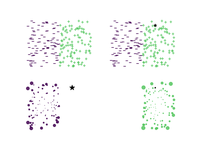
3.2 Magnitude for active learning

Next, we will describe how we can use magnitude and the weight vector to define a query strategy for an active learning algorithm. As stated in (Settles 2009), “The key idea behind active learning is that a machine learning algorithm can achieve greater accuracy with fewer training labels if it is allowed to choose the data from which it learns.”
Approaches that minimize the number of human feedback needed to train machine learning models have sparked renewed interested due to the cost of labeling and the the fact that recent deep-learning-based approaches need handle large amounts of training data to achieve optimal performance. Let (the labeled dataset) and the (unlabeled dataset) be two subsets of the available pool of training data , with and . An iteration of the algorithm will pick some points in to be labeled by an oracle (transferring them to ). The current model will be then updated using the new updated dataset and its corresponding labels.
For simplicity we will state the algorithm for a binary classification problem i.e. when , however it can be trivially extended to a multi-class problem.
The intuition behind the algorithm is simple: at each iteration , we assign every training data point to one of the sets or according to its predicted label by the current classifier . We will calculate the corresponding weight vectors and . Then, we choose to label (submit to an oracle for labeling) the point with the minimum value (interior point) and the with the maximum value (likely to be in the boundary) for both sets and . By choosing this way we are aiming to: (a) reinforce, validate and refine high confidence classifier information (labels) acquired in prior iterations (exploitation) and (b) to acquire labels in the predicted class boundaries where our classifier confidence is potentially lower (exploration). The proposed active learning algorithm is stated below.
Where denotes all components of the vector in absolute value. We present some numerical experiments in Section 4.
3.3 Magnitude for Outlier Detection
In this section we give an algorithm that uses the values of the weight vector of a set to find outliers in a dataset. As we have seen, the weight vector serves as a boundary detector for a data set. But if the boundary is not well defined because there are outlier data points, we can use the weight to mark points as outliers. Suppose we have a data set , and wish to determine if a new point should be considered an outlier with respect to . By looking at the value , we can see if adding increased the magnitude substantially, thereby greatly extending the "border" of . By Lemma 3.1.3 in (Leinster 2013) we have that .
Care must be taken, however; both the points on the boundary of the data set, and the outlier points will have high weight relative to the interior of the data set. Thus we collect all the points in whose weight is below a threshold (here we take median weight plus 1.5 times standard deviation), and denote this subset as , the inliers. The points of not in we call outlier candidates, and denote as . Next, for each with less than a user-defined threshold , we move from to . Then we have our final decomposition of the data set into inliers and outliers: . We record this algorithm in Algorithm 3.
In Figure 4 we have the results of this algorithm using synthetic data. Inlier data was generated from two Gaussian distributions, and outliers were drawn from a uniform distribution.
Remark.
It can be noted that the NULL class prediction algorithm described in Section 3.1 can be viewed as a type of online outlier detection algorithm. If the same paradigm is used when there is a single class, we obtain an outlier detection algorithm that is trained on data that only contains inliers.

4 Results
4.1 Classification Experiments
To test the classification algorithm, we ran a set of ten experiments across 5 classic benchmark datasets from the UCI repository, a synthetic two-dimensional checkerboard dataset, as well as the scikit-learn digit and iris datasets, and multiple classifiers. Each experiment consisted of using a random stratified splitting method to partition the the data set into a training set consisting of 70% of the data, and a testing set consisting of the remaining 30%. The classifiers were trained without fine-tuning any parameters; the basic algorithm presented in 1 with ARGMAX for DECIDE and absolute value for , and the defaults in scikit-learn (Pedregosa et al. 2011) for all parameters in the other algorithms. Table 1 records the average and standard deviation of the accuracy on the testing dataset for all classifiers.
Remark.
Our model performed quite similarly to -nearest neighbors in our experiments, which is quite remarkable given the dramatic differences between the algorithms. We also note the promise it implies: our initial attempt at using the boundary detection properties of the weighting vector in a machine learning setting have matched the performance of a well-established and widely-used model. We believe this will be improved upon and expanded as techniques using the weighting vector are adopted more widely.
| dataset | K-Neighbors | Logistic Reg. | Rand. Forest | SVM | Weight |
|---|---|---|---|---|---|
| 2-d checkerboard | 0.92 0.02 | 0.51 0.04 | 0.94 0.01 | 0.62 0.04 | 0.92 0.01 |
| clevedata.mat | 0.82 0.04 | 0.85 0.02 | 0.82 0.03 | 0.84 0.03 | 0.84 0.03 |
| dimdata.mat | 0.94 0.01 | 0.95 0.01 | 0.95 0.00 | 0.96 0.00 | 0.93 0.01 |
| housingdata.mat | 0.87 0.02 | 0.87 0.03 | 0.87 0.02 | 0.87 0.03 | 0.87 0.02 |
| ionodata.mat | 0.84 0.05 | 0.89 0.02 | 0.94 0.02 | 0.95 0.02 | 0.81 0.08 |
| iris | 0.94 0.04 | 0.87 0.05 | 0.94 0.04 | 0.96 0.03 | 0.85 0.13 |
| sklearn digits | 0.97 0.01 | 0.96 0.01 | 0.95 0.01 | 0.98 0.01 | 0.97 0.00 |
| ticdata.mat | 0.85 0.02 | 0.69 0.03 | 0.93 0.02 | 0.88 0.02 | 0.78 0.03 |
To demonstrate the NULL class label capabilities, we trained the magnitude classifier on examples of six and nine from the scikit-learn digits dataset, then predicted on images of ones, sixes, and nines. The confusion matrix with a NULL class threshold of is shown in table 2.
| null | 6 | 9 | |
| null | 53 | 0 | 1 |
| 6 | 1 | 53 | 0 |
| 9 | 1 | 0 | 54 |
4.2 Active learning Experiments


In order to assess the effectiveness of the weighting-vector-based active learning (AL) algorithm proposed in Section 3.2, we compared Algorithm 2 to the simplest but highly effective and most commonly used query AL framework: uncertainty sampling (Lewis & Gale 1994). In this framework, the AL algorithm queries the instances for which it is least certain about how to label (i.e. for many algorithms or where the decision function is close to ). For simplicity we used a kernelized Ridge regression model (Cristianini & Shawe-Taylor 2000) (also refer as to LS-SVM (Suykens & Vandewalle 1999) or proximal SVM (Fung & Mangasarian 2001)). Laplacian kernels were used both as magnitude to calculate the weighting vector and as classification kernel ( with . At each iteration of Algorithm 2 the classifier learned after obtained labels from the oracle has the form , where is the bias term.
We performed experiments on five classic benchmark datasets from the UCI repository taking 67% of the data as training pool and the remaining 33% as a testing set. Note that the weighing-vector-inspired algorithm chooses points per iterations so we picked the four more uncertain points for the uncertainty sampling algorithm to be fair.
Figure 5 shows average performance curves over 100 runs. The performance from the weighting vector algorithm seems to perform better in four out of the five datasets and slightly worse on the Galaxy dim. and Checkerboard datasets.
5 Conclusions
We apply the concepts of metric space magnitude and weighting vector to a wide variety of classical machine learning tasks. We introduce practical algorithms that are suited to these tasks, and we demonstrate performance that is competitive with, and in many cases, surpasses the performance of benchmark methods. Additionally, we introduce the notion that the weighting vector can accurately identify boundaries on scattered data that lives in a Euclidean space.
Prior work in the field of metric space magnitude has generally been theoretical and focused on the magnitude functional itself, and the properties of the weighting vector have been overshadowed. Practical aspects of metric space magnitude and the weighting vector is still an emergent field. Since magnitude and the weighting vector are well-defined for an extraordinarily wide class of sets, we believe that one natural aim of future work would be to develop vector weighting and magnitude into a robust, unifying foundation for the analysis of familiar, but also highly unusual, spaces.
References
- Barceló & Carbery (2018) Barceló, J. and Carbery, A. On the magnitudes of compact sets in Euclidean spaces. American Journal of Mathematics, 140(2):449–494, 2018. doi: 10.1353/ajm.2018.0011. URL https://muse.jhu.edu/article/688522.
- Cristianini & Shawe-Taylor (2000) Cristianini, N. and Shawe-Taylor, J. An Introduction to Support Vector Machines and Other Kernel-based Learning Methods. Cambridge University Press, 2000.
- Edelsbrunner et al. (2002) Edelsbrunner, H., Letscher, D., and Zomorodian, A. Topological persistence and simplification. Discrete & Computational Geometry, 28(4):511–533, Nov 2002. ISSN 1432-0444. doi: 10.1007/s00454-002-2885-2.
- Folland (1999) Folland, G. Real analysis: modern techniques and their applications. Pure and applied mathematics. Wiley, 1999. ISBN 9780471317166.
- Fung & Mangasarian (2001) Fung, G. and Mangasarian, O. L. Proximal support vector machine classifiers. In KDD ’01, 2001.
- Leinster (2013) Leinster, T. The magnitude of metric spaces. Documenta Mathematica, 18:857–905, 2013.
- Leinster & Shulman (2017) Leinster, T. and Shulman, M. Magnitude homology of enriched categories and metric spaces, 2017. URL https://arxiv.org/abs/1711.00802.
- Lewis & Gale (1994) Lewis, D. D. and Gale, W. A. A sequential algorithm for training text classifiers. CoRR, abs/cmp-lg/9407020, 1994.
- Meckes (2013) Meckes, M. Positive definite metric spaces. Positivity, 17:733–757, Sept 2013. doi: 10.1007/s11117-012-0202-8.
- Meckes (2015) Meckes, M. W. Magnitude, diversity, capacities, and dimensions of metric spaces. Potential Analysis, 42(2):549–572, 2015.
- Otter (2018) Otter, N. Magnitude meets persistence. Homology theories for filtered simplicial sets, 2018. URL https://arxiv.org/abs/1807.01540.
- Pedregosa et al. (2011) Pedregosa, F., Varoquaux, G., Gramfort, A., Michel, V., Thirion, B., Grisel, O., Blondel, M., Prettenhofer, P., Weiss, R., Dubourg, V., Vanderplas, J., Passos, A., Cournapeau, D., Brucher, M., Perrot, M., and Duchesnay, E. Scikit-learn: Machine Learning in Python . Journal of Machine Learning Research, 12:2825–2830, 2011.
- Scopigno et al. (2004) Scopigno, R., Zorin, D., Carlsson, G., Zomorodian, A., Collins, A., and Guibas, L. Persistence barcodes for shapes, 2004.
- Settles (2009) Settles, B. Active learning literature survey. Technical report, University of Wisconsin-Madison Department of Computer Sciences, 2009.
- Solow & Polasky (1994) Solow, A. R. and Polasky, S. Measuring biological diversity. Environmental and Ecological Statistics, 1(2):95–103, Jun 1994. ISSN 1573-3009. doi: 10.1007/BF02426650.
- Suykens & Vandewalle (1999) Suykens, J. and Vandewalle, J. Least squares support vector machine classifiers. Neural Processing Letters, 9:293–300, 06 1999.
- Zomorodian & Carlsson (2004) Zomorodian, A. and Carlsson, G. Computing persistent homology. In Proceedings of the Twentieth Annual Symposium on Computational Geometry, SCG ’04, pp. 347–356, New York, NY, USA, 2004. Association for Computing Machinery. ISBN 1581138857. doi: 10.1145/997817.997870.