Mitigating measurement errors in multi-qubit experiments

Quantum computing experiments are beginning a shift from few-qubit demonstrations of entangling gates and short quantum circuits to larger multi-qubit quantum algorithms attempting to address practically important computational problems. Although available devices are noisy, error mitigation methods have emerged as a possible near-term solution of the fault-tolerance problem Temme et al. 2017; Li and Benjamin 2017; Endo et al. 2018; Otten and Gray 2018; Bonet-Monroig et al. 2018. Error mitigation schemes are particularly attractive because they introduce no overhead in terms of the number of qubits and gates. These methods have recently enabled a reliable simulation of shallow quantum circuits on a noisy hardware without resorting to quantum error correcting codes Kandala et al. 2019; Havlíček et al. 2019. The key idea behind error mitigation is to combine outcomes of multiple experiments in a way that cancels the contribution of noise to the quantity of interest, see Temme et al. 2017; Li and Benjamin 2017; Endo et al. 2018 for details.

Readout errors introduced by imperfect qubit measurements are often the dominant factor limiting scalability of near-term devices. Here we introduce methods for mitigating readout errors for a class of quantum algorithms, where measurement outcomes are only used for computing mean values of observables. Notable examples of such algorithms are variational quantum eigensolvers Peruzzo et al. 2014; Kandala et al. 2017, quantum machine learning Havlíček et al. 2019, and tomography of entangled states DiCarlo et al. 2010. However, our techniques are not applicable to single-shot measurements. The latter are indispensable to many applications such as quantum teleportation, measurement-based computation, and quantum error correction.

Prior work Chen et al. 2019; Chow et al. 2010; Ryan et al. 2015; Merkel et al. 2013; Chow et al. 2012 demonstrated that readout errors in quantum devices based on superconducting qubits can be well understood in terms of purely classical noise models. Such models describe a noisy $n$-qubit measurement by a matrix of transition probabilities $A$ of size $2^{n}\times 2^{n}$ such that $A_{y,x}$ is the probability of observing a measurement outcome $y$ provided that the true outcome is $x$. It is common to simplify the noise model further by assuming that the noise acts independently on each qubit Sun and Geller 2018; Kandala et al. 2017. This defines a tensor product noise model such that $A$ is a tensor product of $2\times 2$ noise matrices. The model depends on $2n$ error rates describing single-qubit readout errors $0\to 1$ and $1\to 0$. The open-source software package, Qiskit Aleksandrowicz et al. 2019, provides a toolkit for calibrating $A$ and mitigating readout errors for either a tensor product or a general noise model.

Although the tensor product noise model is appealingly simple, it leaves aside cross-talk errors encountered in real-world setups. Cross-talk during readout can arise from the underlying qubit-qubit coupling, and spectral overlap of readout resonators with stray couplings or multiplexing Heinsoo et al. 2018. Here we introduce a correlated noise model based on Continuous Time Markov Processes (CTMP). The corresponding noise matrix has the form $A=e^{G}$, where $G$ is a sum of local operators generating single- and two-qubit readout errors such as $01\to 10$, $11\to 00$, etc. The model depends on $2n^{2}$ error rates.

Measurement calibration aims at learning the unknown parameters of a noise model. This is achieved by preparing a set of well-characterized input states (we use the standard basis vectors) and repeatedly performing $n$-qubit measurements on each input state. We show how to extract parameters of the considered noise models from the calibration data using simple analytic formulas. The number of input states required to calibrate the tensor product and CTMP noise models scales linearly with the number of qubits $n$.

Once parameters of the noise model are known, error mitigation proceeds by applying the inverse noise matrix to a probability vector that represents the noisy measurement outcomes. We show how to sidestep the explicit computation of the inverse noise matrix, which may be prohibitive for a large number of qubits. Instead, we follow ideas of Temme et al. 2017 and cancel errors by sampling noise matrices from a suitable quasi-probability distribution. The total error mitigation overhead, including the number of measurements and the cost of classical post-processing, scales as $e^{4\gamma}poly(n)$, where $\gamma$ is a parameter quantifying the noise strength, as formally defined below. For example, if each qubit independently undergoes a bit-flip readout error with probability $\epsilon$ then $\gamma=n\epsilon$. Thus our methods are practical whenever $\gamma$ is a small constant. For comparison, all previously studied readout error mitigation techniques require manipulations with probability vectors of size $2^{n}$ which limits their scalability. Importantly, both tensor product and CTMP error mitigation methods provide an unbiased estimator of the ideal mean value to be measured. For a fixed number of qubits, the cost of approximating the ideal mean value with a specified error tolerance $\delta$ scales as $\delta^{-2}$.

The proposed error mitigation techniques are demonstrated using a $20$-qubit IBM Quantum device. The device has a few-percent readout error rate. For small number of qubits ($n\leq 7$), a comparison is performed between the full noise matrix $A$, the tensor product, and the CTMP noise models. It is found that the CTMP model provides a considerably more accurate approximation of the readout noise. Error mitigated stabilizer measurements of $n$-qubit graph states are reported for $n\leq 12$. Finally, we perform error-mitigated stabilizer measurements on $20$-qubit states generated by low-depth random Clifford circuits. The classical post-processing associated with the error mitigation, including the measurement calibration and the noise inversion steps, can be done on a laptop in a few-second time frame for each of these experiments. Note that the error mitigation runtime is crucial for VQE-type algorithms Kandala et al. 2017 where quantum mean value estimation is repeatedly used in a feedback loop.

Let us briefly discuss the previous work. Seif et al Seif et al. 2018 considered a system of trapped-ion qubits and the problem of discriminating between different basis states based on data collected by an array of photon detectors. It was shown that a neural network trained on the measurement calibration data can realize a high-fidelity state discrimination Seif et al. 2018. It remains to be seen whether similar methods can address the problem of high-precision mean value estimation considered here. Our techniques build off earlier work from Kandala et al Kandala et al. 2017 and are most closely related to the work of Sun and Geller Sun and Geller 2018; Geller 2020; Geller and Sun 2020 who showed how to characterize readout errors in multi-qubit devices. In particular, Ref. Sun and Geller 2018 introduced a noise model based on single- and two-qubit correlation functions which can be viewed as an analogue of the CTMP model considered here. Ref. Maciejewski et al. 2019 elucidated how performance of readout error mitigation methods is affected by the quality of the measurement calibration, number of measurement samples, and the presence of coherent (non-classical) measurement errors, see also Chen et al. 2019. Ref. Nachman et al. 2019 pointed out a surprising connection between quantum readout error mitigation methods and unfolding algorithms used in high energy physics to cope with a finite resolution of particle detectors Cowan 2002. However the classical processing cost of unfolding methods may be prohibitive for multi-qubit experiments since they require manipulations with exponentially large probability vectors. Applications of the noise matrix inversion method in the context of variational quantum algorithms are discussed in Hamilton and Pooser 2019.

After completion of the present paper we became aware of a closely related work by Hamilton, Kharazi et al. Hamilton et al. 2020 which developed a scalable characterization of readout errors based on a cumulant expansion. The latter can be viewed as a counterpart of the CTMP noise model considered here. Namely, both methods provide a recipe for combining single- and two-qubit noise matrices into the full noise matrix describing a multi-qubit device.

The paper is organized as follows. Section II defines an error-mitigated mean value of an observable and shows that it provides an unbiased estimator of the ideal mean value. The tensor product and CTMP noise models are discussed in Sections III,IV. The parameters of these noise models can be extracted from the measurement calibration data as described in Section V. The experimental demonstration of our error mitigation methods is reported in Section VI. Appendices A,B,C prove technical lemmas used in the main text and provide additional details on the implementation of our algorithms. The experimental hardware is described in Appendix D.

Let $\rho$ be the output state of a (noisy) quantum circuit acting on $n$ qubits. Our goal is to measure the expected value of a given observable $O$ on the state $\rho$ within a specified precision $\delta$. For simplicity, below we assume that the observable $O$ is diagonal in the standard basis and takes values in the range $[-1,1]$, that is,

Consider $M$ independent experiments where each experiment prepares the state $\rho$ and then measures each qubit in the standard basis. Let $s^{i}\in\{0,1\}^{n}$ be the string of measurement outcomes observed in the $i$-th experiment. In the absence of measurement errors one can approximate the mean value $\mathrm{Tr}(\rho O)$ by an empirical mean value

By Hoeffding’s inequality, $|\mu-\mathrm{Tr}(\rho O)|\leq\delta$ with high probability (at least $2/3$) if we choose $M=4\delta^{-2}$. Furthermore, $\mu$ is an unbiased estimator of $\mathrm{Tr}(\rho O)$.

Suppose now that measurements are noisy. The most general model of a noisy $n$-qubit measurement involves a POVM with $2^{n}$ elements $\{\Pi_{x}\}$ labeled by $n$-bit strings $x$. The probability of observing a measurement outcome $x$ is given by $P(x)=\mathrm{Tr}(\rho\Pi_{x})$. In the ideal case one has $\Pi_{x}=|x\rangle\langle x|$ while in the presence of noise $\Pi_{x}$ could be arbitrary positive semi-definite operators that obey the normalization condition $\sum_{x}\Pi_{x}=I$. To enable efficient error mitigation, we make a simplifying assumption that all POVM elements $\Pi_{x}$ are diagonal in the standard basis, that is,

for some stochastic matrix $A$ of size $2^{n}$. In other words, $\langle y|A|x\rangle$ is the probability of observing an outcome $y$ provided that the true outcome is $x$. For example, suppose $n=1$ and

Then the probability of measuring $1$ on a qubit prepared in the state $|0\rangle$ is $10\%$. The probability of measuring $0$ on a qubit prepared in the state $|1\rangle$ is $20\%$. For brevity, we shall refer to such readout errors as $0\to 1$ and $1\to 0$ respectively. In this section we assume that the matrix $A$ is known (this assumption is relaxed in Section V). By analogy with Eq. (1), define an error-mitigated empirical mean value as

A proof of the lemma is given in Appendix A. By Hoeffding’s inequality, $|\xi-\mathrm{Tr}(\rho O)|\leq\delta$ with high probability (at least $2/3$) if the number of measurements is

Recall that $M\sim\delta^{-2}$ in the ideal case. Thus the quantity $\Gamma^{2}$ can be viewed as an error mitigation overhead. In other words, error mitigation increases the number of measurements required to achieve a given precision $\delta$ by a factor of $\Gamma^{2}$ compared with the case of ideal measurements.

Consider first a simple case when $A$ is a tensor product of $2\times 2$ stochastic matrices,

Here $\epsilon_{j}$ and $\eta_{j}$ are error rates describing readout errors $0\to 1$ and $1\to 0$ respectively. The error-mitigated mean value $\xi$ defined in Eq. (2) can be easily computed when the observable $O$ has a tensor product form,

For example, $O$ could be a product of Pauli $Z$ operators on some subset of qubits. Alternatively, $O$ could project some subset of qubits onto $0$ or $1$ states. Define a single-qubit state $|e\rangle=|0\rangle+|1\rangle$. From Eqs. (2,5) one gets

Here $s^{i}\in\{0,1\}^{n}$ is the outcome observed in the $i$-th measurement and $s^{i}_{j}\in\{0,1\}$ is $j$-th bit of $s^{i}$. The single-qubit matrix element that appears in Eq. (6) can be computed in constant time for any fixed pair $i,j$. Thus one can compute $\xi$ in time $\approx nM$, that is, the classical post-processing runtime is linear in the number of qubits and the number of measurements. The above algorithm is generalized to arbitrary observables $O$ in Appendix C. The algorithm has runtime $\approx nM\tau$, where $\tau$ is the cost of computing the observable $O(x)$ for a given $x$.

Suppose the noise is weak such that $\epsilon_{j},\eta_{j}\leq 1/2$ for all $j$. Substituting the definition of $A$ into Eq. (3) one gets

We show how to extract the error rates $\epsilon_{j}$ and $\eta_{j}$ from the readout calibration data in Section V. Then Eqs. (4,7) determine the number of measurements $M$, as a function of the desired precision $\delta$. Assuming that $\epsilon_{j},\eta_{j}\ll 1$ one gets $\Gamma\approx e^{2\gamma}$, where $\gamma$ is the noise strength defined as

The error mitigation overhead thus scales as $\Gamma^{2}\approx e^{4\gamma}$.

How can one extend the tensor product noise model to account for correlated (cross-talk) errors ? A natural generalization of a tensor product operator is a Matrix Product Operator (MPO) Schollwöck 2011. Unfortunately, we empirically observed that MPO-based noise models poorly agree with the experimental data, unless the MPO bond dimension is unreasonably large. Noise models based on neural networks provide another possible extension Seif et al. 2018. However, training such noise models and computing error-mitigated mean values in a few-second time frame might not be possible for multi-qubit experiments. Instead, here we propose noise models based on Continuous Time Markov Processes (CTMP) Gillespie 1977.

Define a CTMP noise model as a stochastic matrix $A$ of size $2^{n}\times 2^{n}$ such that ¹¹ 1 Although our definition makes no reference to time, one can express $A$ as a solution of a differential equation $\dot{A}(t)=GA(t)$ with the initial condition $A(0)=I$. Thus $G$ serves as a generator of a continuous time Markov process such that $\langle y|G|x\rangle$ is the rate of transitions from a state $x$ to a state $y\neq x$.

where $e^{G}=\sum_{p=0}^{\infty}G^{p}/p!$ is the matrix exponential, $r_{i}\geq 0$ are error rates, and $G_{i}$ are single-qubit or two-qubit operators from the following list

Each operator $G_{i}$ generates a readout error on some bit or some pair of bits. The right column shows the number of ways to choose qubit(s) acted upon by a generator. The negative terms in $G_{i}$ ensure that $A$ is a stochastic matrix. The CTMP model depends on $2n^{2}$ parameters $r_{i}$, as can be seen by counting the number of generators $G_{i}$ of each type. We show how to extract the error rates $r_{i}$ from the readout calibration data in Section V. Furthermore, the tensor product model Eq. (5) is a special case of CTMP with $r_{i}=0$ for all two-qubit errors. Indeed, in this case Eq. (8) defines a tensor product of single-qubit stochastic matrices

Here we assume that $\epsilon+\eta<1$.

Next let us show how to compute the error-mitigated mean value $\xi$ defined in Eq. (2). Since $\xi$ itself is only a $\delta$-estimate of the true mean value $\mathrm{Tr}(\rho O)$, it suffices to approximate $\xi$ within an error $\approx\delta$. We use a version of the well-known Gillespie algorithm Gillespie 1977 for simulating continuous Markov processes combined with the following lemma proved in Appendix B.

Here $\Gamma$ is the quantity defined in Eq. (3). Suppose we have found a decomposition Eq. (9) for the inverse CTMP noise matrix $A^{-1}=e^{-G}$. Then the error-mitigated mean value $\xi$ defined in Eq. (2) can be approximated using the following algorithm.

Algorithm 1: $T\leftarrow 4\delta^{-2}\|c\|_{1}^{2}$ for $t=1$ to $T$ do   Sample $i\in[M]$ uniformly at random   Sample $\alpha$ from the distribution $q_{\alpha}=|c_{\alpha}|/\|c\|_{1}$   Sample $x$ from the distribution $\langle x|S_{\alpha}|s^{i}\rangle$   $\xi_{t}\leftarrow\mathrm{sgn}(c_{\alpha})O(x)$ end for return $\xi^{\prime}=T^{-1}\|c\|_{1}\sum_{t=1}^{T}\xi_{t}$

Here $c_{\alpha},S_{\alpha}$ are the same as in Lemma 2. We claim that the output this algorithm satisfies $|\xi^{\prime}-\xi|\leq\delta$ with high probability (at least $2/3$). Indeed, substituting Eq. (9) into Eq. (2) one gets

that is,

Here $i\in[M]$ is picked uniformly at random, $\alpha$ is sampled from $q_{\alpha}$, and $x(i,\alpha)$ is sampled from the distribution $\langle x|S_{\alpha}|s^{i}\rangle$ with fixed $i,\alpha$. Accordingly, a random variable $\|c\|_{1}\mathrm{sgn}(c_{\alpha})O(x(i,\alpha))$ is an unbiased estimator of $\xi$ with the variance at most $\|c\|_{1}^{2}$. By Hoeffding’s inequality, $|\xi^{\prime}-\xi|\leq\delta$ with high probability (at least $2/3$).

In the special case of the tensor product noise one can efficiently compute a decomposition $A^{-1}=\sum_{\alpha}c_{\alpha}S_{\alpha}$ defined in Lemma 2 with $\|c\|_{1}=\Gamma$, see Appendix C. This yields an instantiation of Algorithm 1 that computes a $\delta$-estimate of $\xi$ in time roughly

Here $M$ is the number of measurements determined by Eq. (4). Further details on the implementation of Algorithm 1 for the tensor product noise can be found in Appendix C.

Next, let us show how to implement Algorithm 1 for the CTMP model $A=e^{G}$. Define a parameter

We shall see that the error mitigation overhead introduced by the CTMP method scales as $e^{4\gamma}$. To avoid a confusion with individual error rates $r_{i}$ we shall refer to the quantity $\gamma$ as the CTMP noise strength. The function $-\langle x|G|x\rangle$ can be viewed as a classical Ising-like Hamiltonian with two-spin interactions. Although finding the maximum energy of such Hamiltonians is NP-hard in the worst case, this can be easily done for moderate system sizes, say $n\leq 50$, using heuristic optimizers such as simulated annealing. Below we assume that the noise strength $\gamma$ has been already computed.

First we note that $\gamma\geq 0$ since $G$ has non-positive diagonal elements. Define a matrix

Using Eq. (13) and the fact that $G$ has zero column sums, one can check that $B$ is a stochastic matrix. Furthermore,

where

Clearly, $S_{\alpha}$ is a stochastic matrix for any integer $\alpha\geq 0$. Thus Eqs. (15,16) provide a stochastic decomposition of $A^{-1}$ stated in Lemma 2 with the $1$-norm

The probability distribution

is the Poisson distribution with the mean $\gamma$. Substitute the decomposition of Eqs. (15,16) into Algorithm 1. The only non-trivial step of the algorithm is sampling $x$ from the distribution

This amounts to simulating $\alpha$ steps of a Markov Chain with the transition matrix $B$. Note that $B$ is a sparse efficiently computable matrix. More precisely, each column of $B$ has $\approx n^{2}$ non-zero elements. Thus one can simulate a single step of the Markov chain in time $\approx n^{2}$. Since $\mathbb{E}(\alpha)=\gamma$, simulating $\alpha$ steps of the Markov chain on average takes time $\approx\gamma n^{2}$. The overall runtime of Algorithm 1 becomes

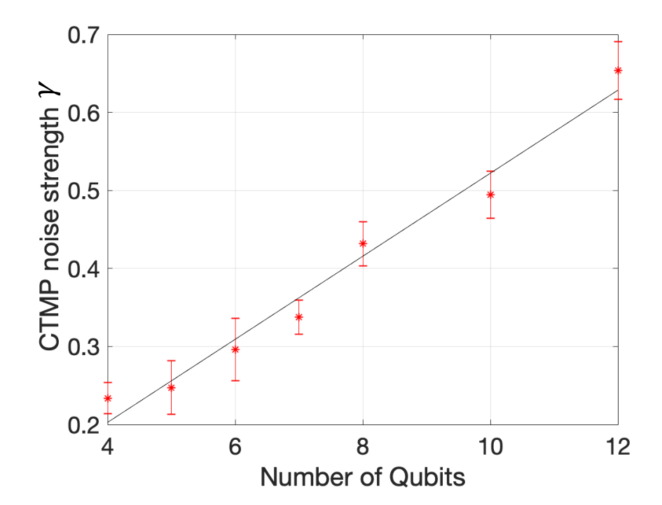
Here we used Eq. (17). Assuming that cross-talk errors result from short-range interactions between qubits, one should expect that each qubit participates in a constant number of generators $G_{i}$ independent of $n$. If this is the case, each column of $G$ has at most $Cn$ non-zero elements for some constant $C$. Then $\gamma\leq C\epsilon n$, where $\epsilon=\max_{i}r_{i}$ is the maximum error rate. Thus the exponential term in the runtime of Algorithm 1 becomes $e^{4C\epsilon n}$. Experimental data presented in Section VI are consistent with a linear scaling $\gamma\sim n$, see Fig. 5.

Calibration aims at learning parameters of the noise model from the experimental data. A single calibration round initializes the $n$-qubit register in a basis state $|x\rangle$ and performs a noisy measurement of each qubit, keeping the record of the measured outcome $y$. Let $m(y,x)$ be the number of rounds with the input state $x$ and the measured output state $y$. We fix some set of input states ${\cal C}\subseteq\{0,1\}^{n}$ and perform $N_{\mathsf{cal}}$ calibration rounds for each input state $x\in{\cal C}$. Thus $\sum_{y}m(y,x)=N_{\mathsf{cal}}$ if $x\in{\cal C}$ and $m(y,x)=0$ if $x\notin{\cal C}$. The calibration requires $N_{\mathsf{cal}}\cdot|{\cal C}|$ experiments in total.

Learning the full noise matrix requires calibration of each possible input state, i.e. ${\cal C}=\{0,1\}^{n}$. Let $A_{\mathsf{full}}$ be the empirical estimate of the full noise matrix, i.e.

where $x,y\in\{0,1\}^{n}$.

To learn error rates of the tensor product or the CTMP model it suffices to calibrate a small subset of basis states. Consider first the tensor product model. To ensure that each possible single-qubit readout error is probed on some input state, we assume that for any qubit $j$ the set ${\cal C}$ contains at least one state $x$ with $x_{j}=0$ and at least one state with $x_{j}=1$. Let $\epsilon_{j}$ and $\eta_{j}$ be the rates of errors $0\to 1$ and $1\to 0$ on the $j$-th qubit, see Eq. (5). We set

For example, $\epsilon_{j}$ is the fraction of calibration rounds that resulted in a readout error $0\to 1$ on the $j$-th qubit among all rounds with $x_{j}=0$. Let $A_{\mathsf{tp}}$ be the tensor product noise matrix defined by the rates $\epsilon_{j},\eta_{j}$ and Eq. (5).

Next consider the CTMP model. Recall that the model is defined by $2n^{2}$ error rates describing readout errors $0\leftrightarrow 1$, $01\leftrightarrow 10$, and $00\leftrightarrow 11$. To ensure that each possible two-qubit readout error is probed on some input state, we assume that for any pair of qubits $j\neq k$ and for any $v_{j},v_{k}\in\{0,1\}$ the set ${\cal C}$ contains at least one state $x$ such that $x_{j}=v_{j}$ and $x_{k}=v_{k}$. For example, ${\cal C}$ could include bit strings $0^{n}$, $1^{n}$, and all weight-$1$ strings. Fix a pair of qubits $j\neq k$. Given a bit string $x\in\{0,1\}^{n}$, let $x_{\mathsf{in}}\in\{0,1\}^{2}$ be the restriction of $x$ onto the bits $j,k$ and $x_{\mathsf{out}}\in\{0,1\}^{n-2}$ be the restriction of $x$ onto all remaining bits $i\notin\{j,k\}$. We choose CTMP error rates on qubits $j,k$ by defining a local noise matrix $A(j,k)$ and fitting $A(j,k)$ with a two-qubit CTMP model. More formally, $A(j,k)$ is a stochastic matrix of size $4\times 4$ with matrix elements

Here $v,w\in\{0,1\}^{2}$. In words, $\langle w|A(j,k)|v\rangle$ is the fraction of calibration rounds that resulted in a readout error $v\to w$ on qubits $j,k$ and no errors on qubits $i\notin\{j,k\}$ among all rounds with $x_{\mathsf{in}}=v$ that resulted in no errors on qubits $i\notin\{j,k\}$. Let

be the matrix logarithm of $A(j,k)$. We choose the branch of the $\log$ function such that $G(j,k)=0$ if $A(j,k)=I$. The rates of two-qubit errors occurring on the qubits $j,k$ are chosen as shown in the following table.

Here $G^{\prime}(j,k)$ is a matrix obtained from $G(j,k)$ by setting to zero all negative off-diagonal elements. Let $r_{j}^{0\to 1}$ and $r_{j}^{1\to 0}$ be the rates of single-qubit readout errors $0\to 1$ and $1\to 0$ occurring on the $j$-th qubit. We set

Here we noted that two-qubit errors $01\leftrightarrow 10$ or $00\leftrightarrow 11$ on qubits $j,k$ can only be generated by the local noise matrix $A(j,k)$. Meanwhile, single-qubit errors $0\leftrightarrow 1$ on the $j$-th qubit can be generated by any local noise matrix $A(j,k)$ with $k\neq j$. The above definition of single-qubit error rates amounts to taking the average over all such possibilities. Let $A_{\mathsf{ctmp}}$ be the CTMP noise model defined by the above error rates and Eq. (8).

The calibration method described above is well-defined only if the set of input states ${\cal C}$ is complete in the sense that any two-bit readout error can be probed on some input state $x\in{\cal C}$. More formally, let us say that a set of $n$-bit strings ${\cal C}$ is complete if for any pair of bits $1\leq a<b\leq n$ and for any bit values $\alpha,\beta\in\{0,1\}$ there exists at least one string $x\in{\cal C}$ such that $x_{a}=\alpha$ and $x_{b}=\beta$, see Fig. 1 for an example. Below we describe complete sets of input states used in our experiments.

All experiments are performed using $n$-qubit registers of the 20-qubit IBM Quantum device called $\mathsf{ibmq\_johannesburg}$, see Appendix D for details. Only the chosen $n$-qubit register is used for readout calibration. The unused qubits are initialized in the $|0\rangle$ state in each calibration round. Measurement outcomes on the unused qubits are ignored. All experiments were performed with $N_{\mathsf{cal}}=8192$ calibration rounds.

First, let us discuss how well the tensor product (TP) and the CTMP models approximate the readout noise observed in the experiment. We quantify the difference between a pair of $n$-qubit noise matrices $A$ and $A^{\prime}$ using the Total Variation Distance (TVD)

The TVD provides an upper bound on the probability of distinguishing output distributions $A|p\rangle$ and $A^{\prime}|p\rangle$ for any input distribution $p$. This enables a comparison between noise models in the worst-case scenario rather than for a specific quantum state and a specific observable.

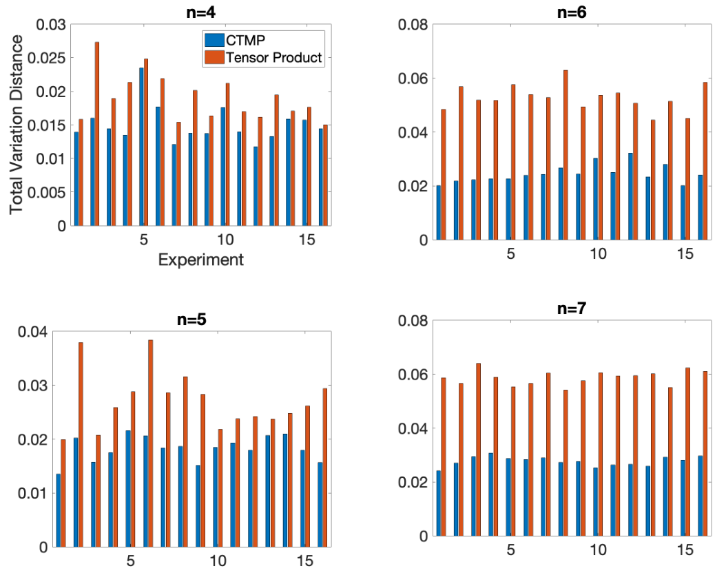
For small number of qubits, $n\leq 7$, all three calibration methods described in Section V have been performed. Let $A_{\mathsf{full}}$ be the full noise matrix. Let $A_{\mathsf{tp}}$ and $A_{\mathsf{ctmp}}$ be the noise matrices predicted by the TP and CTMP models with weight-$2$ calibration. Fig. 2 shows the observed distances $\mathsf{TVD}(A_{\mathsf{full}},A_{\mathsf{ctmp}})$ and $\mathsf{TVD}(A_{\mathsf{full}},A_{\mathsf{tp}})$ for $n=4,5,6,7$ qubits (with the qubits chosen for $n<7$ consisting of subsets of the $n=7$ case) and $16$ independent experiments per each number of qubits. It indicates that the CTMP model provides a more accurate approximation of the readout noise achieving 2X reduction in the TVD metric for $n=6,7$ qubits. The increased separation between TP and CTMP models for larger numbers of qubits indicates that readout crosstalk is larger in the additional qubits used for the circuits with more qubits. Note that this improvement comes at no additional cost since both models have access to exactly the same calibration data set.

In order to compare the methods of measurement mitigation on relevant quantum circuits, we use graph states as an example of a highly entangled state that can serve as a benchmark for quantum devices. We estimate the fidelity with stabilizer measurements for $n$-qubit graph states Raussendorf and Briegel 2001 of the form

The corresponding graph is a path with $n$ vertices. The state $|G_{n}\rangle$ is a stabilizer state with the stabilizer group ${\cal S}$ generated by Pauli operators $S_{1}=X_{1}Z_{2}$, $S_{n}=Z_{n-1}X_{n}$, and $S_{j}=Z_{j-1}X_{j}Z_{j+1}$ for $1<j<n$. Let $\rho$ is an approximate version of $|G_{n}\rangle$ prepared in the lab by executing the quantum circuit Eq. (21). The fidelity $\langle G_{n}|\rho|G_{n}\rangle$ can be estimated by picking a random element of the stabilizer group $S\in{\cal S}$ and measuring its mean value on the state $\rho$,

A comparison between the error-mitigated fidelity $F$ obtained using the full $A$-matrix, TP, and CTMP methods with weight-$1$ calibration is shown on Fig. 3(a). We also show raw values of $F$ obtained without error mitigation. The full $A$-matrix model was only used for $n\leq 7$. The data suggests that CTMP provides much more accurate estimates of the fidelity, compared with the TP model which systematically over-estimates the fidelity. The mean value of each stabilizer was estimated by measuring $M=8192$ copies of the graph state $|G_{n}\rangle$. The entire experiment (calibration and mean value measurements) was repeated $16$ times in order to estimate error bars.

For the six-qubit graph state, there are few enough stabilizers that we can measure all of them. Let $\xi_{\mathsf{full}}(S)$, $\xi_{\mathsf{tp}}(S)$, and $\xi_{\mathsf{ctmp}}(S)$ be the error-mitigated mean values $\mathrm{Tr}(\rho S)$ of a stabilizer $S$ obtained using the full $A$-matrix, the TP, and the CTMP method respectively. Fig. 3(b) shows the differences $\xi_{\mathsf{full}}(S)-\xi_{\mathsf{tp}}(S)$ and $\xi_{\mathsf{full}}(S)-\xi_{\mathsf{ctmp}}(S)$ averaged over stabilizers of the same weight, $|S|$. It can be seen that the TP method systematically over-estimates the mean values for stabilizers with the weight $3,4,5,6$, while CTMP shows a much better agreement with the full $A$-matrix method. The difference between CTMP and TP increases for higher weight stabilizers, which we expect to be more sensitive to correlated readout errors. Fig. 4 (a) shows the combined rate of correlated two-qubit errors $01\leftrightarrow 10$ and $00\leftrightarrow 11$, as described by the CTMP model, for each pair of qubits in the chosen 12-qubit register. It can be seen that some pairs of qubits, such as $(7,8)$, experience correlated errors with a few-percent rate.

Recall that the error mitigation overhead introduced by the CTMP method is roughly $e^{4\gamma}$, where $\gamma$ is the noise strength defined in Eq. (13). Fig. 5 shows the noise strength $\gamma$ observed in the graph state experiments as a function of the number of qubits. Error bars were estimated from $16$ independent experiments. The data is consistent with a linear scaling, $\gamma\approx 0.05n$, and with single qubit readout fidelities of a few percent (see Appendix D for more details on the readout errors in the hardware). We observed $\gamma\leq 0.7$ for all experiments reported above. The error mitigation overhead is therefore at most $e^{4\cdot 0.7}\leq 20$, indicated a factor of $20$ increase in the number of measurements required.

Our last experiment demonstrates error mitigated stabilizer measurements on an entangled $20$-qubit state $|\psi\rangle$ generated by a random depth-$4$ Clifford circuit. The circuit consists of two layers of CNOT gates on nearest-neighbor pairs of qubits and two layers of single-qubit Clifford operators, see Fig. 6. Such state $|\psi\rangle$ can be specified by a group of Pauli-type stabilizers $S\in\pm\{I,X,Y,Z\}^{\otimes 20}$ such that $S|\psi\rangle=|\psi\rangle$. We have measured mean values $\langle\psi|S|\psi\rangle$ for $\approx 500$ stabilizers $S$ chosen randomly such that the weight of $S$ varies between $1$ and $20$. In the absence of readout and gate errors one has $\langle\psi|S|\psi\rangle=1$ for all stabilizers $S$. Our results for the error mitigated mean values $\langle\psi|S|\psi\rangle$ obtained with the TP and CTMP methods and Hadamard-type calibration are shown on Fig. 6. In contrast to the graph state experiment, error rates associated with correlated two-qubit errors $01\leftrightarrow 10$ and $00\leftrightarrow 11$ observed in the $20$-qubit experiment are less than $1\%$ for all pairs of qubits, see Fig. 4(b). Accordingly, the difference between error mitigated mean values obtained using the TP and CTMP methods is less pronounced.

The $20$-qubit experiment showcases the scalability of our method. For example, computing the error-mitigated mean value of a $20$-qubit stabilizer using the CTMP method with $T=10^{6}$ samples in Algorithm 1 takes about $2$ seconds on a laptop computer (recall that $T$ affects the cost of a classical post-processing but not the number of experiments). Extracting CTMP error rates from the $20$-qubit calibration data takes about $1$ second. Thus we expect that our methods can be scaled up to a larger number of qubits.

We introduced scalable methods of mitigating readout errors in multi-qubit experiments. Our methods are capable of mitigating correlated cross-talk errors and enable efficient implementation of the calibration and the noise inversion steps. The proposed error mitigation methods are demonstrated experimentally for measurements of up to $20$ qubits. We believe that our techniques will be useful for many near term quantum applications, and their scalability will be increasingly important as the problem sizes become larger.