Turbocharging Treewidth-Bounded
Bayesian Network Structure
LearningThanks: This is the full version of a paper to appear in
the proceedings of AAAI-21, the Thirty-Fifth AAAI Conference on
Artificial Intelligence. The authors acknowledge the support by the FWF
(projects P32441 and W1255) and by the WWTF (project
ICT19-065).
Abstract
We present a new approach for learning the structure of a treewidth-bounded Bayesian Network (BN). The key to our approach is applying an exact method (based on MaxSAT) locally, to improve the score of a heuristically computed BN. This approach allows us to scale the power of exact methods—so far only applicable to BNs with several dozens of random variables—to large BNs with several thousands of random variables. Our experiments show that our method improves the score of BNs provided by state-of-the-art heuristic methods, often significantly.
1 Introduction
Bayesian network structure learning is the notoriously difficult problem of discovering a Bayesian network (BN) that optimally represents a given set of training data [6]. Since exact inference on a BN is exponential in the BN’s treewidth [17], one is particularly interested in learning BNs of bounded treewidth. However, learning a BN of bounded treewidth that optimally fits the data (i.e., with the largest possible score) is, in turn, an NP-hard task [16]. This predicament caused the research on treewidth-bounded BN structure learning to split into two branches:
- 1.
Heuristic Learning (see, e.g., Elidan and Gould 2009, Nie et al. 2015, Scanagatta et al. 2016, Scanagatta et al. 2018, Benjumeda et al. 2019), which is scalable to large BNs with thousands of random variables but with a score that can be far from optimal, and
- 2.
Exact Learning (see, e.g., Berg et al. 2014, Korhonen and Parviainen 2013, Parviainen et al. 2014), which learns optimal BNs but is scalable only to a few dozen random variables.
In this paper, we combine heuristic and exact learning and take the best of both worlds.
The basic idea for our approach is to first compute a BN with a heuristic method (the global solver), and then to apply an exact method (the local solver) to parts of the heuristic solution. The parts are chosen small enough that they allow an optimal solution reasonably quickly with the exact method. Although the basic idea sounds compelling and reasonably simple, its realization requires several conceptual contributions and new results.
For the global solver, any heuristic algorithm for treewidth-bounded BN learning, such as the recent algorithms k-MAX [31] or ETL [3]. The local solver’s task is significantly more complex than treewidth-bounded BN structure learning, as several additional constraints need to be incorporated. Namely, it is not sufficient that the BN computed by the local solver is acyclic. We need fortified acyclicity constraints that prevent cycles that run through the other parts of the BN, which have not been changed by the local solver. Similarly, it is not sufficient that the local BN is of bounded treewidth. We need fortified treewidth constraints that prevent the local BN from introducing links between a diverse set of nodes that, together with the other parts of the BN, which have not been changed by the local solver, increase the treewidth.
Given these additional requirements, we propose a new local solver BN-SLIM (SAT-based Local Improvement Method), which satisfies the fortified constraints. We formulate a fortified version of the treewidth-bounded BN structure learning problem. In Theorem 1, we show that we can express the fortified constraints with certain virtual arcs and virtual edges. The virtual arcs represent directed paths that run outside the local instance; with these virtual arcs we can ensure fortified acyclicity. The virtual edges represent essential parts of a global tree decomposition using which we can ensure bounded treewidth.
The new formulation of the local problem is well-suited to be expressed as a MaxSAT (Maximum Satisfiability) problem and hence allows us to harvest the power of state-of-the-art MaxSAT solvers (which received a significant performance gain over the last decade). A distinctive feature of our encoding is that, in contrast to the virtual edges, the virtual arcs are conditional and depend on the local solver’s solution.
1.1 Results
We implement BN-SLIM and evaluate it empirically on a large set of benchmark data sets, consisting between 64 and 10,000 random variables and for the treewidth bounds 2, 5, and 8. As the global solver, we use the state-of-the-art heuristic algorithms for treewidth-bounded BN learning k-MAX [31], and two variants of ETL [3]. k-MAX improves over the k-greedy algorithm [30], which was the first algorithm for treewidth-bounded structure learning that scaled to thousands of random variables. The more recent algorithm ETL is reported to perform better than k-MAX in many cases [3].
We consider about a hundred benchmark data sets based on real-world and synthetic data sets, ranging up to 4000 random variables in our experiments. First we run the global solvers on the data sets, followed by running BN-SLIM to improve the score of the DAG they provided. Our results show that after running BN-SLIM for 5 minutes, 73% of all DAGs could be improved; by extending the time for BN-SLIM to 15 minutes, the improvement extends to 82%. We also notice that, overall, BN-SLIM can improve the lower treewidth DAGs more efficiently.
Since k-MAX is an anytime algorithm that can produce better and better solutions over time, we can directly compare the improvements achieved by k-MAX after some initial run with the improvements achieved by BN-SLIM. Our experiments show that after an initial run of k-MAX for 30 minutes, it is highly beneficial to stop k-MAX and hand the torch over to BN-SLIM, as BN-SLIM provides improvements at a significantly higher rate. According to the BIC metric, which was used by Scanagatta et al. 2018 for comparing treewidth-bounded BN structure learning algorithms, the results are “extremely positive” in favor of BN-SLIM over k-MAX in a vast majority of the experiments.
We cannot perform such a direct comparison between ETL and BN-SLIM, since the available implementation of ETL does not support an anytime run, but stops after a certain time. Hence, we let ETL finish, and run BN-SLIM afterwards for 30 minutes. The achieved improvement in terms of the BIC metric is “extremely positive” for 84% of all DAGs computed by two variants of ETL.
1.2 Related work
The first SAT-encoding for finding the treewidth of a graph was proposed by Samer and Veith 2009. Fichte et al. 2017 proposed the first SAT-based local improvement method for treewidth, using the Samer-Veith encoding as the local solver. Recently, SAT encodings have been proposed for other graph and hypergraph width measures [9, 10, 20, 32]. So far, there have been four concrete approaches that use the SLIM framework, one for branchwidth [19, 21], one for treewidth [8], one for treedepth [26] and one for decision trees [33].
Several exact approaches to treewidth-bounded BN structure learning have been proposed. Korhonen and Parviainen 2013 proposed a dynamic-programming approach, and Parviainen et al. 2014 proposed a Mixed-Integer Programming approach. Berg et al. 2014 proposed a MaxSAT approach by extending the basic Samer-Veith encoding for treewidth. Our approach for BN-SLIM uses a similar general strategy, but we encode acyclicity differently. Moreover, BN-SLIM deals with the fortified constraints in terms of virtual edges and virtual arcs.
Since the exact methods are limited to small domains, Nie et al. 2015, Nie et al. 2016 suggested heuristic approaches that scale up to hundreds of random variables. The k-greedy algorithm proposed by Scanagatta et al. 2016 at NIPS’16 provided a breakthrough, consistently yielding better DAGs than its competitors and scaling up to several thousand of random variables. As mentioned above, k-MAX [31] is a more recent improvement over k-greedy. More recently, Benjumeda et al. 2019 came up with the ETL algorithms, based on local search within the space of structures called elimination trees. These algorithms perform better than k-MAX and k-greedy in many cases.
2 Preliminaries
2.1 Structure learning
We consider the problem of learning the structure (i.e., the DAG) of a BN from complete data set of instances over a set of categorical random variables . The goal is to find a DAG where is the set of nodes (one for each random variable) and is the set of arcs (directed edges). The value of a score function determines how well a DAG fits the data; the DAG , together with local parameters, forms the BN [15].
We assume that the score is decomposable, i.e., being constituted by the sum of the individual random variables’ scores. Hence we can assume that the score is given in terms of a score function that assigns each node and each subset a real number , the score of for . The score of the entire DAG is then
where denotes the parent set of in . This setting accommodates several popular scores like AIC, BDeu, and BIC [1, 13, 34]. If and are two potential parent sets of a random variable such that and , then we can safely disregard the potential parent set of . Consequently, we can disregard all nonempty potential parent sets of with a score . Such a restricted score function is a score function cache.
2.2 Treewidth
Treewidth is a graph invariant that provides a good indication of how costly probabilistic inference on a BN is. Treewidth is defined on undirected graphs and applies to BNs via the moralized graph of the DAG underlying the BN under consideration, where
A tree decomposition of a graph is a pair , where is a tree and is a function that assigns each tree node a set of vertices of such that the following conditions hold:
- T1
-
For every edge of there is a tree node such that .
- T2
-
For every vertex of , the set of tree nodes with induces a non-empty subtree of .
The sets are called bags of the decomposition , and is the bag associated with the tree node . The width of a tree decomposition is the size of a largest bag minus . The treewidth of , denoted by , is the minimum width over all tree decompositions of .
The treewidth-bounded BN structure learning problem takes as input a set of nodes, a decomposable score function on , and an integer , and it asks to compute a DAG of treewidth , such that is maximal.
3 Local improvement
Consider an instance of the treewidth-bounded BN structure learning problem, and assume we have computed an initial solution heuristically, together with a tree decomposition of width of the moralized graph .
We select a subtree such that the number of vertices in is at most some budget . The budget is a parameter that we specify beforehand, such that the subinstance induced by is small enough to be solved optimally by an exact method, which we call the local solver. The local solver computes for each a new parent set, optimizing the score of the resulting DAG .
Consider the induced DAG , where . The local solver ensures that the following conditions are met:
- C1
is acyclic.
- C2
The moral graph has treewidth .
We assume that the local solver certifies C2 by producing a tree decomposition of of width , which can be used by the global solver.
The two conditions stated above are not sufficient to ensure that is acyclic and that treewidth of remains bounded by . Acyclicity can be violated by cycles formed by the combination of the new incoming arcs of vertices in together with old arcs that are kept from . The treewidth can increase by a number that is linear in .
Hence, we need additional side conditions, which we will formulate using the following additional concepts.
Let us call a vertex a boundary vertex if there exists a tree node such that , i.e., it occurs in some bag outside . We call the other vertices in internal vertices, and the vertices in external vertices. Further, we call two boundary vertices adjacent if there exists a tree node such that , i.e., both vertices occur together in some bag outside . It is easy to see that any pair of adjacent boundary vertices occur together in a bag of as well.
For any two adjacent boundary vertices , we call a virtual edge. Let be the set of all virtual edges. These virtual edges form a clique and serve a similar purpose as the marker cliques used in other work [8]. The extended moral graph is obtained from by adding all virtual edges.
For any two adjacent boundary vertices , we call a virtual arc, if contains a directed path from to , where all the vertices on the path, except for and , are external. Let be the set of all virtual arcs.
We can now formulate the side conditions.
- C3
is a tree decomposition of the extended moral graph .
- C4
For each , if contains external vertices, then there is some such that .
- C5
The digraph is acyclic.
We note that condition C4 implies that in , all parents of an internal vertex are internal.
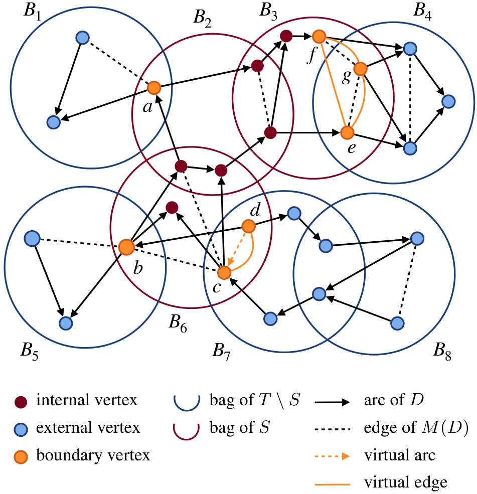
Theorem 1.
If all the conditions C1–C5 are satisfied, then is acyclic, the treewidth of is at most , and the score of is at least the score of .
Proof.
We define a new tree decomposition of as follows. Let be the connected components of , i.e., the ’s are the subtrees of that we get when deleting the subtree . Let , , and observe that each external vertex belongs to exactly one of the sets . Let , , be the set of boundary vertices in . We observe that all the vertices in are mutually adjacent boundary vertices and occur together in a bag of and in a bag , for , as we can take and to be the two neighboring tree nodes of with and . We also observe that each forms a clique in the extended moral graph .
Recall that by assumption, the local solver provides a tree decomposition of of width . Additionally, by condition C3, is also a tree decomposition of , and hence, by a basic property of tree decompositions (see, e.g., Bodlaender and Möhring 1993), there must exist a bag , , with . Hence we can define as the tree we get by connecting the disjoint trees with the edges , . We extend from to by setting for .
Claim 1.
is a tree decomposition of of width .
To prove the claim, we show that satisfies the conditions T1 and T2.
Condition T1. There are two reasons for an edge to belong to : first, because of an arc and second, because of two arcs . First case: . If and are both external, then for some . If neither nor is external, then , and since is a tree decomposition of , for some . If is external but isn’t, then the arc was already present in , as the parents of external vertices didn’t change. Hence, since is a tree decomposition of , it follows that for some . If is external but isn’t, it follows from C4 that for some . Second case: . If , then , and so for some , since is a tree decomposition of . If but or , then C4 implies that for some . If , then are two adjacent boundary vertices, hence is a virtual edge which, by C3, means for some . We conclude that T1 holds.
Condition T2. Let . If is external, then there is exactly one , such that . Since we do not change the tree decomposition of , condition T2 carries over from to . Similarly, if is internal, then does not appear in any bag for , hence condition T2 carries over from to . It remains to consider the case where is a boundary vertex. The tree nodes with are connected, because satisfies T2, and for , the tree nodes for which are connected, since satisfies T2. By construction of , if , then there are neighboring tree nodes and with . Hence all the tree nodes with are connected, and T2 also holds for boundary vertices.
To conclude the proof of the claim, it remains to observe the width of cannot exceed the widths of or , hence the width of is at most .
Claim 2.
is acyclic.
To prove the claim, suppose to the contrary that contains a directed cycle . The cycle cannot lie entirely in , nor can it lie entirely in , because and are acyclic. Hence, contains at least one arc from and at least one arc from . Let and , for , be these arcs, such that they appear on in the order , , , . It is possible that or . We observe that the vertices on the path from to on all belong to some . Hence and are adjacent boundary vertices, and contains all the arcs , . However, the cycle contains also the paths from to , for , which only run through vertices in . These paths, together with the virtual arcs form a cycle which lies in . This contradicts C5 which requires that this digraph be acyclic. Hence the claim holds.
Claim 3.
The score of is at least the score of .
We observe that by taking we have a solution that satisfies all the required conditions and maintains the score. ∎
4 Implementing the local improvement
In this section, we first discuss how the set representing the subinstance is constructed. Then we provide a detailed explanation of the MaxSAT encoding that is responsible for solving the subinstance.
4.1 Constructing the subinstance
For this section, we follow the same notation as used in the previous section. To construct the subinstance, we initialize the subtree with a tree node picked at random from . We then expand by performing a bread-first search from and adding a new tree node to as long as the size of does not exceed the budget. Next, we compute for the chosen . Finally, we prune the parent sets of each vertex so as to only retain those parent sets which satisfy conditions C3 and C4. This can be done by first checking, for each parent set, if the required tree node is present , and if it does, we record the set of virtual arcs that are imposed by this parent set as long as none of the virtual arcs are self-loops. For each and , we denote by the set of imposed virtual arcs when has the parent set in . We denote by , the collection of parent sets of node that remain after this pruning process. Notice that, under this pruning, all remaining parent sets satisfy C4. Also note that, since is conditional on the chosen parent sets, it cannot be precomputed.
Further, since we intend to solve the subinstance using a MaxSAT encoding, we need to ensure that the score of each parent set is non-negative. Recall that only contains those non-empty parent sets whose score is at least that of the empty parent set. Thus, we may assume that the empty parent set has the lowest score among all the parents of a certain vertex. Consequently, we can adjust the score function by setting for and , which implies that for all and .
4.2 MaxSAT encoding
We now describe the weighted partial MaxSAT instance that encodes conditions C1–C5. We build on top of the SAT encoding proposed by Samer and Veith 2009. The only difference in our case is that there are no explicit edges and hence we do not require the corresponding clauses. Instead, the edges of the moralized graph are dependent on and decided by other variables that govern the DAG structure. For convenience, let denote the size of the subinstance, i.e., . A part of the encoding is based on the elimination ordering of a tree decomposition (see, e.g., Samer and Veith 2009).
The main variables used in our encoding are
- •
variables represent for each node the chosen parent set ,
- •
variables represent the topological ordering of ,
- •
variables represent the elimination ordering of the tree decomposition,
- •
variables represent the arcs in the moralized graph , along with the fill-in edges (see Samer and Veith 2009).
Since and represent linear orderings, we enforce transitivity of these variables by means of the clauses
To prevent self-loops in the moralized graph, we add the clauses
For each node , and parent set , the variable is true if and only if is the parent set of . Since each node must have exactly one parent set, we introduce the cardinality constraint
Next, for each node , parent set , and , if is the parent set of then must precede in the topological ordering. Hence we add the clause
Similarly, for each node , parent set , and , if is the parent set of then we must add an arc in the moralized graph respecting the elimination ordering between and , as follows:
Next, we encode the moralization by adding an arc between every pair of parents of a node, using the following clauses
Now, we encode the fill-in edges, with the following clauses
Lastly, to bound the treewidth, we add a cardinality constraint on the number of outgoing arcs for each node as follows
To complete the basic encoding, for every node , and every parent set we add a soft clause weighted by the score of the parent set as follows
To speed up the solving, we encode that for every pair of nodes, at most one of the arcs between them can exist. We add the following redundant clauses
Now, we describe the additional clauses required to satisfy the fortified constraints, and thus conditions C3 and C5. For every virtual edge , we introduce a forced arc depending on the elimination ordering using the following pair of clauses
This takes care of the fortified treewidth constraints, satisfying C3 and ensuring that the edge for some . Finally, we add the clauses that encode the forced arcs . For each , , and , we add the clause
which forces the virtual arc if is the parent set of in , thereby handling the fortified acyclicity constraints and ensuring that C5 is satisfied.
This concludes the definition of the MaxSAT instance, to which we will refer as . We refer to the weight of a satisfying assignment of as the sum of the weights of all the soft clauses satisfied by . Let . To each satisfying assignment of we can associate for each the corresponding parent set, which in turn determines a directed graph . Due to Theorem 1, the treewidth of is bounded by , and is acyclic. By construction of , the weight of equals . Conversely, if we pick new parent sets for the vertices in such that all the conditions C1–C5 are satisfied, then by construction of , the corresponding truth assignment satisfies , and its weight is . In particular, let be the weight of the truth assignment which corresponds to the parent sets of as defined by the input DAG . We summarize these observations in the following theorem.
Theorem 2.
has a solution of weight if and only if there are new parent sets for the vertices in giving rise to a DAG with .
5 Experimental evaluation
In this section, we describe the experiments conducted to analyze the performance of the local improvement algorithm. The current state-of-the-art heuristic algorithms for solving the treewidth-bounded BN structure learning problem are the k-MAX algorithm by Scanagatta et al. 2018 and the ETL algorithms by Benjumeda et al. 2019 (available as two variants–the default variant ETLd and the poly-time variant ETLp), therefore, we analyze the benefit of applying BN-SLIM on top of these algorithms. It is worth noting that both k-MAX and BN-SLIM are anytime algorithms, i.e., they run indefinitely long and can be halted at any instant to output the best solution found so far; ETL, on the other hand, as per the available implementation, is deterministic and terminates when it fails to find any new improvements. This distinction affects the nature of the experiments conducted to draw a comparison between the different algorithms. However, for the most part, we closely follow the experimental setup (including data sets, timeouts, comparison metrics) used by Scanagatta et al. 2018 to compare k-MAX with previous approaches.
Since BN-SLIM needs an initial heuristic solution, we enlist either k-MAX, ETLd, or ETLp for this purpose. We denote by BN-SLIM(X), the algorithm which applies BN-SLIM on an initial solution provided by X where X . We run all our experiments with treewidth bounds 2, 5, 8 for each data set following Scanagatta et al. 2018. All reported BN-SLIM results are averages over three random seeds (see supp. material for details).
5.1 Setup
We run all our experiments on a 4-core Intel Xeon E5540 2.53 GHz CPU, with each process having access to 8GB RAM. We use UWrMaxSat as the MaxSAT-solver primarily due to its anytime nature (available at the 2019 MaxSAT Evaluation webpage11 1 https://maxsat-evaluations.github.io/2019/descriptions.html). We tried other solvers but found that UWrMaxSat works best for our use case. We use the BNGenerator package [14] in conjunction with the BBNConvertor tool [11] to generate and reformat random Bayesian Networks. We also use the implementation of the k-MAX algorithm available as a part of the BLIP package [29]. For the ETL algorithms we use the software made available22 2 https://github.com/marcobb8/et-learn by Benjumeda et al. 2019. We implement the local improvement algorithm in Python 3.6.9, using the NetworkX 2.4 graph library [12]. The source code along with the experiment data is available publicly at https://github.com/aditya95sriram/bn-slim.
We first conducted a preliminary analysis on 20 data sets to find out the best values for the budget (maximum number of random variables in a subinstance) and the timeout (per MaxSAT call) of BN-SLIM. We tested out budget values 7, 10, and 17, and timeout values 1s, 2s, and 5s, and finally settled on a budget of 10 and a timeout of 2 seconds for our experiments.
5.2 Data sets
We consider 99 data sets for our experiments. 84 of these come from real-world benchmarks. These are based on the benchmarks introduced by Lowd and Davis 2010, Van Haaren and Davis 2012, Bekker et al. 2015, Larochelle et al. 2010, a subset of which has been used by Scanagatta et al. 2018. These benchmarks are publicly available33 3 https://github.com/arranger1044/DEBD in the form of pre-partitioned data sets. There are three data sets corresponding to each of the 28 benchmarks (see Table 1).
The remaining 15 data sets are classified as synthetic as they are obtained by drawing 5000 samples from known BNs (see Table 2). Five of these BNs are commonly used in the literature as benchmarks44 4 https://www.bnlearn.com/bnrepository/, and we generated the remaining 10 BNs randomly using the BNGenerator tool with more random variables than the previously mentioned data sets. Overall, the collection of data sets provides a wide variety of the data’s nature and the different parameters.
Both k-MAX and BN-SLIM take a score function cache as input, while ETL requires the samples themselves and computes the required scores on-the-fly. We thus compute the score function cache using the scoring module provided as a part of ETL’s source code. More specifically, we first obtain the parent set tuples using independence selection (available in the BLIP package), and then we recompute the scores for these tuples using ETL’s scoring module. This cache is used as input to both BN-SLIM and k-MAX. This provides a level playing field and improves comparability between the different algorithms.
While computing these score function caches, the scoring function module was unable to process two data sets and hence we discarded these two data sets. The final list of data sets is shown in Tables 1 and 2. Further, k-MAX crashes for 3 data sets and hence we disregard these for any experiments involving k-MAX or BN-SLIM(k-MAX).
| Name | Name | Name | |||
|---|---|---|---|---|---|
| NLTCS | 16 | Connect 4 | 126 | EachMovie | 500 |
| MSNBC | 17 | OCR Letters | 128 | WebKB | 839 |
| KDDCup2k | 65 | RCV-1 | 150 | Reuters-52 | 889 |
| Plants | 69 | Retail | 135 | 20 NewsGroup | 910 |
| Audio | 100 | Pumsb-star | 163 | Movie reviews | 1001 |
| Jester | 100 | DNA | 180 | BBC | 1058 |
| Netflix | 100 | Kosarek | 190 | Voting | 1359 |
| Accidents | 111 | MSWeb | 294 | Ad | 1556 |
| Mushrooms | 112 | NIPS | 500 | ||
| Adult | 123 | Book | 500 |
| Name | Name | Name | |||
|---|---|---|---|---|---|
| andes | 223 | r0 | 2000 | r5 | 4000 |
| diabetes | 413 | r1 | 2000 | r6 | 4000 |
| pigs | 441 | r2 | 2000 | r7 | 4000 |
| link | 724 | r3 | 2000 | ||
| munin | 1041 | r4 | 2000 |
5.3 Evaluation metric
For evaluating our algorithm’s performance, we use the same metric as Scanagatta et al. 2018, i.e., BIC, which is the difference between the BIC scores of two solutions. Given a DAG , the BIC score approximates the logarithm of the marginal likelihood of . Thus, given two DAGs and , the difference in their BIC scores approximates the ratio of their respective marginal likelihoods which is the Bayes Factor [27]. A positive BIC score signifies positive evidence towards and a negative BIC score signifies positive evidence towards . The BIC values can be mapped to a scale of qualitative categories [27] as shown in Table 3.
| Category | BIC | Category | BIC |
|---|---|---|---|
| extremely negative | extremely positive | ||
| strongly negative | strongly positive | ||
| negative | positive |
5.4 Experimental results
The primary focus of our experimentation is to analyze the benefit gained by applying BN-SLIM on top of other heuristics and not to compare between the different heuristics. To this end, we run BN-SLIM for 60 minutes on top of the initial solution provided by k-MAX, ETLd, and ETLp and measure the time required for BN-SLIM to obtain a solution that counts as extremely positive evidence with respect to the initial solution. The initial solution by k-MAX is the solution captured at the 30-minute mark, whereas the initial solution by ETL is the final solution obtained upon termination. The maximum time required for computing the initial solution on any individual instance, by both ETLd and ETLp, is around 3.5 hours. For comparison, we let k-MAX continue running for 60 more minutes after it has produced the initial solution.
Fig. 2 shows the results of this analysis. We consider a data set to be significantly improved if BN-SLIM is able to improve by at least 10 BIC points over the initial heuristic solution. We observe that BN-SLIM improves over k-MAX much more efficiently as over ETL. Giving k-MAX more time for computing the initial solution increases this discrepancy even further, as the improvement rate of k-MAX rapidly slows down after 30 minutes. Averaging over all the heuristics, BN-SLIM can produce a solution with extremely positive evidence for 95%, 79%, and 78% of instances for treewidth bounds 2, 5, and 8, respectively.
Fig. 4 shows the BIC values from comparing the BN-SLIM(ETL) solution after 30 minutes to the corresponding initial solution by ETL. We can see that BN-SLIM(ETL) can secure extremely positive evidence for a significant number of data sets across all tested treewidth bounds, with a smaller treewidth being more favorable.
Due to the anytime nature of k-MAX, we can compare it against BN-SLIM(k-MAX) in a “race.” We run both simultaneously for one hour, where out of the time allotted to BN-SLIM(k-MAX), 30 minutes are used to generate the initial solution, and the remaining 30 minutes are used to improve this initial solution. Fig. 3 shows the BIC values of comparing k-MAX and BN-SLIM(k-MAX) at the one hour mark. Similar to BN-SLIM(ETL) we observe that BN-SLIM(k-MAX) outperforms k-MAX on a significant number of instances, and on all instances for treewidth 2.
The experimental evaluation demonstrates BN-SLIM approach’s effectiveness and the combined power as a heuristic method of BN-SLIM(k-MAX) and BN-SLIM(ETL).
6 Conclusion
With BN-SLIM, we have presented a novel method for improving the outcome of treewidth-bounded BN structure learning heuristics. We have demonstrated its robustness and performance by applying BN-SLIM to the solution provided by the state-of-the-art heuristics k-MAX, ETLd, and ETLp. The approach of BN-SLIM is based on exact reasoning via MaxSAT, which is fundamentally different from the mentioned heuristics. Consequently, both approaches complement each other, and their combination provides significantly better solutions than any of the heuristics alone. Simultaneoulsy, the combination still scales to large instances with thousands of random variables, which are far out of reach for exact methods alone. Thus, BN-SLIM combines the best of both worlds.
The highly encouraging experimental outcome suggests several avenues for future work, which include the development of more sophisticated subinstance selection schemes, the inclusion of variable fidelity sampling (crude for the global solver, fine-grained for the local solver), as well as more complex collaboration protocols between local and global solver in a distributed setting.
References
- Akaike [1974] Hirotugu Akaike. A new look at the statistical model identification. IEEE transactions on automatic control, 19(6):716–723, 1974.
- Bekker et al. [2015] Jessa Bekker, Jesse Davis, Arthur Choi, Adnan Darwiche, and Guy Van den Broeck. Tractable learning for complex probability queries. In Advances in Neural Information Processing Systems, pages 2242–2250, 2015.
- Benjumeda et al. [2019] Marco Benjumeda, Concha Bielza, and Pedro Larrañaga. Learning tractable bayesian networks in the space of elimination orders. Artificial Intelligence, 274:66–90, 2019.
- Berg et al. [2014] Jeremias Berg, Matti Järvisalo, and Brandon M. Malone. Learning optimal bounded treewidth bayesian networks via maximum satisfiability. In Proceedings of the Seventeenth International Conference on Artificial Intelligence and Statistics, AISTATS 2014, Reykjavik, Iceland, April 22-25, 2014, volume 33 of JMLR Workshop and Conference Proceedings, pages 86–95. JMLR.org, 2014.
- Bodlaender and Möhring [1993] Hans L. Bodlaender and Rolf H. Möhring. The pathwidth and treewidth of cographs. SIAM J. Discrete Math., 6(2):181–188, 1993. doi: 10.1137/0406014.
- Chickering [1996] David Maxwell Chickering. Learning equivalence classes of Bayesian network structures, 1996.
- Elidan and Gould [2009] Gal Elidan and Stephen Gould. Learning bounded treewidth bayesian networks. In Daphne Koller, Dale Schuurmans, Yoshua Bengio, and Léon Bottou, editors, Advances in Neural Information Processing Systems 21, Proceedings of the Twenty-Second Annual Conference on Neural Information Processing Systems, Vancouver, British Columbia, Canada, December 8-11, 2008, pages 417–424. Curran Associates, Inc., 2009.
- Fichte et al. [2017] Johannes K. Fichte, Neha Lodha, and Stefan Szeider. SAT-based local improvement for finding tree decompositions of small width. In Serge Gaspers and Toby Walsh, editors, Theory and Applications of Satisfiability Testing - SAT 2017 - 20th International Conference, Melbourne, VIC, Australia, August 28 - September 1, 2017, Proceedings, volume 10491 of Lecture Notes in Computer Science, pages 401–411. Springer Verlag, 2017. doi: 10.1007/978-3-319-66263-3_25.
- Fichte et al. [2018] Johannes K. Fichte, Markus Hecher, Neha Lodha, and Stefan Szeider. An SMT approach to fractional hypertree width. In John N. Hooker, editor, Proceedings of CP 2018, the 24rd International Conference on Principles and Practice of Constraint Programming, volume 11008 of Lecture Notes in Computer Science, pages 109–127. Springer Verlag, 2018. doi: 10.1007/978-3-319-98334-9_8.
- Ganian et al. [2019] Robert Ganian, Neha Lodha, Sebastian Ordyniak, and Stefan Szeider. SAT-encodings for treecut width and treedepth. In Stephen G. Kobourov and Henning Meyerhenke, editors, Proceedings of ALENEX 2019, the 21st Workshop on Algorithm Engineering and Experiments, pages 117–129. SIAM, 2019. doi: 10.1137/1.9781611975499.10.
- Guo [2002] Haipeng Guo. BBNConvertor – Bayesian Networks Formats Convertor, 2002. URL http://kdd.cs.ksu.edu/KDD/Groups/Probabilistic-Reasoning/convertor.html.
- Hagberg et al. [2008] Aric A. Hagberg, Daniel A. Schult, and Pieter J. Swart. Exploring network structure, dynamics, and function using NetworkX. In Proceedings of the 7th Python in Science Conference (SciPy2008), pages 11–15, Pasadena, CA USA, August 2008.
- Heckerman et al. [1995] David Heckerman, Dan Geiger, and David Maxwell Chickering. Learning Bayesian networks: The combination of knowledge and statistical data. Machine Learning, 20(3):197–243, 1995.
- Ide [2015] Jaime S. Ide. BNGenerator – A generator for random Bayesian network, 2015. URL http://sites.poli.usp.br/pmr/ltd/Software/BNGenerator.
- Koller and Friedman [2009] Daphne Koller and Nir Friedman. Probabilistic graphical models: principles and techniques. MIT press, 2009.
- Korhonen and Parviainen [2013] Janne H. Korhonen and Pekka Parviainen. Exact learning of bounded tree-width bayesian networks. In Proceedings of the Sixteenth International Conference on Artificial Intelligence and Statistics, AISTATS 2013, Scottsdale, AZ, USA, April 29 - May 1, 2013, volume 31 of JMLR Workshop and Conference Proceedings, pages 370–378. JMLR.org, 2013.
- Kwisthout et al. [2010] Johan Kwisthout, Hans L. Bodlaender, and Linda C. van der Gaag. The necessity of bounded treewidth for efficient inference in bayesian networks. In Helder Coelho, Rudi Studer, and Michael Wooldridge, editors, ECAI 2010 - 19th European Conference on Artificial Intelligence, Lisbon, Portugal, August 16-20, 2010, Proceedings, volume 215 of Frontiers in Artificial Intelligence and Applications, pages 237–242. IOS Press, 2010.
- Larochelle et al. [2010] Hugo Larochelle, Yoshua Bengio, and Joseph Turian. Tractable multivariate binary density estimation and the restricted boltzmann forest. Neural computation, 22(9):2285–2307, 2010.
- Lodha et al. [2016] Neha Lodha, Sebastian Ordyniak, and Stefan Szeider. A SAT approach to branchwidth. In Nadia Creignou and Daniel Le Berre, editors, Theory and Applications of Satisfiability Testing - SAT 2016 - 19th International Conference, Bordeaux, France, July 5-8, 2016, Proceedings, volume 9710 of Lecture Notes in Computer Science, pages 179–195. Springer Verlag, 2016. doi: 10.1007/978-3-319-40970-2_12.
- Lodha et al. [2017] Neha Lodha, Sebastian Ordyniak, and Stefan Szeider. SAT-encodings for special treewidth and pathwidth. In Serge Gaspers and Toby Walsh, editors, Theory and Applications of Satisfiability Testing - SAT 2017 - 20th International Conference, Melbourne, VIC, Australia, August 28 - September 1, 2017, Proceedings, volume 10491 of Lecture Notes in Computer Science, pages 429–445. Springer Verlag, 2017. doi: 10.1007/978-3-319-66263-3_27. URL http://www.ac.tuwien.ac.at/files/tr/ac-tr-17-012.pdf.
- Lodha et al. [2019] Neha Lodha, Sebastian Ordyniak, and Stefan Szeider. A SAT approach to branchwidth. ACM Trans. Comput. Log., 20(3):15:1–15:24, 2019. doi: 10.1145/3326159. URL http://www.ac.tuwien.ac.at/files/tr/ac-tr-19-010.pdf.
- Lowd and Davis [2010] Daniel Lowd and Jesse Davis. Learning markov network structure with decision trees. In 2010 IEEE International Conference on Data Mining, pages 334–343. IEEE, 2010.
- Nie et al. [2015] Siqi Nie, Cassio Polpo de Campos, and Qiang Ji. Learning bounded tree-width bayesian networks via sampling. In Sébastien Destercke and Thierry Denoeux, editors, Symbolic and Quantitative Approaches to Reasoning with Uncertainty - 13th European Conference, ECSQARU 2015, Compiègne, France, July 15-17, 2015. Proceedings, volume 9161 of Lecture Notes in Computer Science, pages 387–396. Springer Verlag, 2015.
- Nie et al. [2016] Siqi Nie, Cassio Polpo de Campos, and Qiang Ji. Learning bayesian networks with bounded tree-width via guided search. In Dale Schuurmans and Michael P. Wellman, editors, Proceedings of the Thirtieth AAAI Conference on Artificial Intelligence, February 12-17, 2016, Phoenix, Arizona, USA, pages 3294–3300. AAAI Press, 2016.
- Parviainen et al. [2014] Pekka Parviainen, Hossein Shahrabi Farahani, and Jens Lagergren. Learning bounded tree-width bayesian networks using integer linear programming. In Proceedings of the Seventeenth International Conference on Artificial Intelligence and Statistics, AISTATS 2014, Reykjavik, Iceland, April 22-25, 2014, volume 33 of JMLR Workshop and Conference Proceedings, pages 751–759. JMLR.org, 2014.
- Peruvemba Ramaswamy and Szeider [2020] Vaidyanathan Peruvemba Ramaswamy and Stefan Szeider. Maxsat-based postprocessing for treedepth. In Helmut Simonis, editor, Principles and Practice of Constraint Programming, pages 478–495, Cham, 2020. Springer International Publishing. ISBN 978-3-030-58475-7.
- Raftery [1995] Adrian E. Raftery. Bayesian model selection in social research. Sociological Methodology, 25:111–163, 1995. ISSN 00811750, 14679531. URL http://www.jstor.org/stable/271063.
- Samer and Veith [2009] Marko Samer and Helmut Veith. Encoding treewidth into SAT. In Theory and Applications of Satisfiability Testing - SAT 2009, 12th International Conference, SAT 2009, Swansea, UK, June 30 - July 3, 2009. Proceedings, volume 5584 of Lecture Notes in Computer Science, pages 45–50. Springer Verlag, 2009.
- Scanagatta [2015] Mauro Scanagatta. BLIP – Bayesian Network learning and inference package , 2015. URL https://ipg.idsia.ch/software/blip.
- Scanagatta et al. [2016] Mauro Scanagatta, Giorgio Corani, Cassio Polpo de Campos, and Marco Zaffalon. Learning treewidth-bounded bayesian networks with thousands of variables. In Daniel D. Lee, Masashi Sugiyama, Ulrike von Luxburg, Isabelle Guyon, and Roman Garnett, editors, Advances in Neural Information Processing Systems 29: Annual Conference on Neural Information Processing Systems 2016, December 5-10, 2016, Barcelona, Spain, pages 1462–1470, 2016.
- Scanagatta et al. [2018] Mauro Scanagatta, Giorgio Corani, Marco Zaffalon, Jaemin Yoo, and U Kang. Efficient learning of bounded-treewidth bayesian networks from complete and incomplete data sets. Int. J. Approx. Reason, 95:152–166, 2018.
- Schidler and Szeider [2020] André Schidler and Stefan Szeider. Computing optimal hypertree decompositions. In Guy Blelloch and Irene Finocchi, editors, Proceedings of ALENEX 2020, the 22nd Workshop on Algorithm Engineering and Experiments, pages 1–11. SIAM, 2020.
- Schidler and Szeider [2021] André Schidler and Stefan Szeider. SAT-based decision tree learning for large data sets. In Proceedings of AAAI’21, the Thirty-Fifth AAAI Conference on Artificial Intelligence. AAAI Press, 2021.
- Schwarz [1978] Gideon Schwarz. Estimating the dimension of a model. The annals of statistics, 6(2):461–464, 1978.
- Van Haaren and Davis [2012] Jan Van Haaren and Jesse Davis. Markov network structure learning: A randomized feature generation approach. In Twenty-Sixth AAAI Conference on Artificial Intelligence, 2012.