Limiting Eigenfunctions of Sturm-Liouville operators Subject to a Spectral Flow

It is well known that the $n$-th eigenfunction of a regular Sturm–Liouville problem, with separable boundary conditions on a finite interval, has precisely $n-1$ interior zeros. Put differently, it has exactly $n$ nodal domains, where the nodal domains of $u$ are defined to be the connected components of the set $\{x:u(x)\neq 0\}$.

In higher dimensions one has the Courant nodal domain theorem, which says the $n$th eigenfunction of the Laplacian, or more generally the Schrödinger operator $-\Delta+V$, has at most $n$ nodal domains. Unlike the one-dimensional case, this is generally a strict inequality: While Courant’s theorem says that $\nu(n)\leq n$ for all $n$, where $\nu(n)$ denotes the number of nodal domains for the $n$-th eigenfunction, for any dimension greater than one it was shown by Pleijel [Ple56] that the equality $\nu(n)=n$ can only hold for finitely many values of $n$.

An eigenfunction for which $\nu(n)=n$ is said to be Courant sharp. For some relative simple domains, such as squares, balls, equilateral triangles and tori, it is possible to completely determine the Courant sharp eigenfunctions. See, for instance, [BHK20, HS16, BH16, BNH17, Lén15, HHOT10, HHOT09] among many others. In general this is a very challenging problem, and there is much that is not known.

The extent to which an eigenfunction is not Courant sharp is measured by its nodal deficiency,

(1)

$$\delta(n):=n-\nu(n).$$

The first explicit formula for the nodal deficiency that we are aware of was given in [BKS12], in terms of the Morse index of an energy function defined on the space of equipartitions. A second formula, in terms of Dirichlet-to-Neumann maps on the nodal set, was obtained in [CJM17] using infinite-dimensional symplectic methods.

The starting point of the current work is [BCM19], in which the nodal deficiency formula of [CJM17] was reinterpreted (and reproved) using a spectral flow approach. The benefit of this approach is that it identifies an explicit mechanism by which low energy eigenfunctions can contribute to the nodal deficiency.

The idea is as follows:

1. (1)

   Fix an eigenfunction $u_{n}$, with eigenvalue $\lambda_{n}$, and define the nodal set $\mathcal{Z}=\overline{\{x:u_{n}(x)=0\}}$;

2. (2)

   Define the family of operators $L(\sigma)=-\Delta+\sigma\delta_{\mathcal{Z}}$ for $\sigma\geq 0$;

3. (3)

   Write the eigenvalues of $L(\sigma)$ in analytic branches $\lambda_{m}(\sigma)$ such that $\lambda_{m}(0)$ are the eigenvalues of $L(0)=-\Delta$.

It is not hard to show that the eigenvalue curves $\lambda_{m}(\sigma)$ are non-decreasing. In particular, $\lambda_{n}(\sigma)$ remains constant, whereas $\lambda_{1}(\sigma),\ldots,\lambda_{n-1}(\sigma)$ are strictly increasing. Of these first $n$ eigenvalue curves, precisely $\nu(n)$ of them will converge to $\lambda_{n}$ as $\sigma\to\infty$, while the remaining $n-\nu(n)$ will converge to values larger than $\lambda_{n}$. Therefore, the nodal deficiency of $u_{n}$ is equal to the number of eigenvalue curves that pass through $\lambda_{n}$ as $\sigma$ ranges from $0$ to $\infty$.

In [BCM19] this spectral flow was analyzed for a Schrödinger operator with separable potential on a rectangular domain, assuming the eigenfunction $u_{n}$ of interest is separable. These assumptions reduce the problem to a one-dimensional one, where the analysis is easier. The main simplification is due to the fact that in one dimension the eigenvalues must be simple, and so the eigenvalue curves cannot intersect as $\sigma$ changes. (In particular, this implies that in one dimension the nodal deficiency is always zero, reproducing the classic result of Sturm.)

While the analysis of [BCM19] completely describes the limiting behavior of the eigenvalues in the separable case, the corresponding eigenfunctions were not studied, as they were not needed to determine the nodal deficiency. The current paper addresses this issue.

This is motivated by the desire to study small perturbations of separable eigenfunctions, for an eigenvalue of multiplicity at least two. For instance, the methods of [BCM19] apply to the Laplacian eigenfunction $\sin(2\pi x)\sin(\pi y)$ on the unit square, but not to the eigenfunction $\sin(2\pi x)\sin(\pi y)+\epsilon\sin(\pi x)\sin(2\pi y)$. In the first case the nodal set is a union of horizontal and vertical lines, so the operator $L(\sigma)$ is separable, while in the latter case the nodal set is more complicated, and a similar ODE reduction is not possible. It should be possible to study the spectral flow for such a non-separable eigenfunction by viewing it as a small perturbation of the separable case, but this will require knowledge of the limiting eigenfunctions in the separable case.

Moreover, understanding the limiting eigenfunctions should lead to additional insight into the spectral flow in general, and the mechanism by which an eigenfunction $u_{m}$ with eigenvalue $\lambda_{m}<\lambda_{n}$ does (or does not) contribute to the nodal deficiency of $u_{n}$.

In order to state our results, we first recall the one-dimensional spectral flow from [BCM19]. Consider the Sturm–Liouville eigenvalue problem

(2)

$$-u^{\prime\prime}(x)+V(x)u=\lambda u(x),\qquad u(0)=u(1)=0.$$

Given the $n$-th eigenfunction $u_{n}$ of (2), the nodal set $\{x\in(0,1):u_{n}(x)=0\}$ consists of $n-1$ points, and hence can be written as $\{x_{k}\}_{k=1}^{n-1}$. For a fixed $n>1$, the spectral flow is defined by the eigenvalue problem

(3)

$$-u^{\prime\prime}(x)+V(x)u(x)+\sigma u(x)\sum_{k=1}^{n-1}\delta(x-x_{k})=\lambda(\sigma)u(x),\qquad u(0)=u(1)=0,$$

parameterized by $\sigma\in[0,\infty)$. Here the potential $V$ has been shifted by adding delta functions of strength $\sigma$ at the zeros of $u_{n}$.

An equivalent formulation, without reference to delta functions, is that $u(x)$ solves the differential equation (2) on each open subinterval $(x_{k-1},x_{k})$ (letting $x_{0}=0$ and $x_{n}=1$ for convenience) with the boundary conditions $u(0)=u(1)=0$ and

(4)

$$u(x_{k}^{+})=u(x_{k}^{-}),\qquad u^{\prime}(x_{k}^{+})-u^{\prime}(x_{k}^{-})=\sigma u(x_{k})$$

for $1\leq k\leq n-1$, where $\pm$ superscripts denote right- and left-hand limits, respectively. These boundary conditions ensure that the eigenfunctions are continuous at $x_{k}$, but have a jump in their derivatives whenever $\sigma>0$ and $u(x_{k})\neq 0$.

The one-dimensional analysis in [BCM19] shows that the eigenvalues $\lambda_{m}(\sigma)$ of (3) depend analytically on $\sigma$, with

$$\lim_{\sigma\to\infty}\lambda_{m}(\sigma)=\lambda_{n},\qquad 1\leq m\leq n,$$

and

$$\lim_{\sigma\to\infty}\lambda_{m}(\sigma)>\lambda_{n},\qquad m>n.$$

This result holds for any continuous potential $V$, and does not rely on explicit formulas for the eigenvalues, which are only available for special choices of $V$. However, it gives no information about the eigenvalues for intermediate values of $\sigma$, or about the eigenfunctions for any values of $\sigma$ other than $0$. In this paper we completely solve this problem for the case $V(x)=0$.

To that end, we consider the eigenvalue problem

(5)

$$-u^{\prime\prime}(x)=\lambda u(x),\ \ \ u(0)=u(1)=0.$$

The eigenfunctions are given by $u_{n}(x)$ = $C_{n}\sin(n\pi x)$, where $C_{n}$ is a constant, with corresponding positive eigenvalues $\lambda_{n}$ = $n^{2}\pi^{2}$, for each $n\in\mathbb{N}$.

We fix $n\geq 2$, and impose the boundary conditions (4) at the zeros of the eigenfunction $u_{n}(x)$ = $\sin(n\pi x)$. The zeros of $u_{n}$ occur at $x_{k}=\tfrac{k}{n}$, where 0 $\leq$ $k$ $\leq$ $n$, $k$ $\in$ $\mathbb{Z}$. At the interior zeros, the boundary conditions from (4) therefore become

(6)

$$u\big(\tfrac{k}{n}^{+}\big)=u\big(\tfrac{k}{n}^{-}\big),\qquad u^{\prime}\big(\tfrac{k}{n}^{+}\big)-u^{\prime}\big(\tfrac{k}{n}^{-}\big)=\sigma u\big(\tfrac{k}{n}\big)$$

for $1\leq k\leq n-1$.

For each $\sigma\geq 0$, we want to examine the behavior of the eigenvalues $\lambda_{m}(\sigma)$ and eigenfunctions $u_{m}(x;\sigma)$ of the equation and boundary conditions given in (5) and (6). In this notation $\lambda_{m}(0)=m^{2}\pi^{2}$, $u_{m}(x;0)=\sin(m\pi x)$, and the eigenvalues $\lambda_{m}(\sigma)$ are simple for any finite $\sigma$. Since $u_{n}(x)=\sin(n\pi x)$ vanishes at the interior nodes $x_{k}$, the $n$-th eigenvalue is constant, $\lambda_{n}(\sigma)=n^{2}\pi^{2}$ for all $\sigma$, and we can also take $u_{n}(x;\sigma)$ to be independent of $\sigma$. However, the same is not true for $\lambda_{m}(\sigma)$ and $u_{m}(x;\sigma)$ for $1\leq m\leq n-1$. Our main theorem provides a description of these eigenvalues and eigenfunctions for all $\sigma\geq 0$.

To obtain the limiting eigenfunctions, which we denote by

(10)

$$u_{m}(x;\infty)=\lim_{\sigma\to\infty}u_{m}(x;\sigma),$$

one can use the fact that $\gamma_{m}(\sigma)\to n\pi$ for $1\leq m\leq n$ to obtain

$$u_{m}(x;\infty)=\left(1+\sum_{j=1}^{k-1}(-1)^{j}A_{j,m}\right)\sin(n \pi x)\quad\text{for }x\in I_{k}$$

from (8), where the coefficients $A_{j,m}=\lim_{\sigma\to\infty}A_{j,m}(\sigma)$ are given by (9). An alternate approach is given below in Corollary 1.3. Along the way we obtain more information about the eigenfunctions, which leads directly to an explicit formula for $u_{m}(x;\infty)$, see (12) and (13).

As $\sigma$ increases, the derivatives of $u_{m}(x;\sigma)$ remain bounded, and so to ensure that the interior condition in (6) continues to hold, the values $u_{m}(x_{k};\sigma)$ must converge to $0$ as $\sigma$ converges to infinity. Our first corollary of Theorem 1.1 is that these values converge to $0$ at the same rate for each node $x_{k}$.

We next define the quantity

(11)

$$F_{k,m}(\sigma)=\int_{I_{k}}u_{m}(x;\sigma)\sin(n \pi x)\,dx,$$

which provides a measure of the weight of $u_{m}(x;\sigma)$ in each interval $I_{k}$. Using Theorem 1.1, we can carefully control its dependence on $\sigma$.

Finally, we examine the behavior of the eigenfunctions as the parameter $\sigma$ approaches infinity. As shown in [BCM19], the eigenvalues $\lambda_{m}(\sigma)$ for $1\leq m\leq n$ all converge to $\lambda_{n}=n^{2}\pi^{2}$ as $\sigma$ tends to infinity. (Note that this is consistent with our implicit expression for the eigenvalues $\lambda_{m}(\sigma)$ from Theorem 1.1.) From Corollary 1.1, this ensures that $u_{m}(x_{k};\sigma)$ converges to zero as $\sigma$ tends to infinity. This means that $u_{m}(x;\infty)$ (defined in (10)) is proportional to $\sin(n\pi x)$ on each interval $I_{k}$, so it can be represented by a vector with $n$ entries, where the $k$th entry of the vector is the coefficient of $\sin(n \pi x)$ on $I_{k}$. Our final corollary of Theorem 1.1 gives an explicit expression for these vectors.

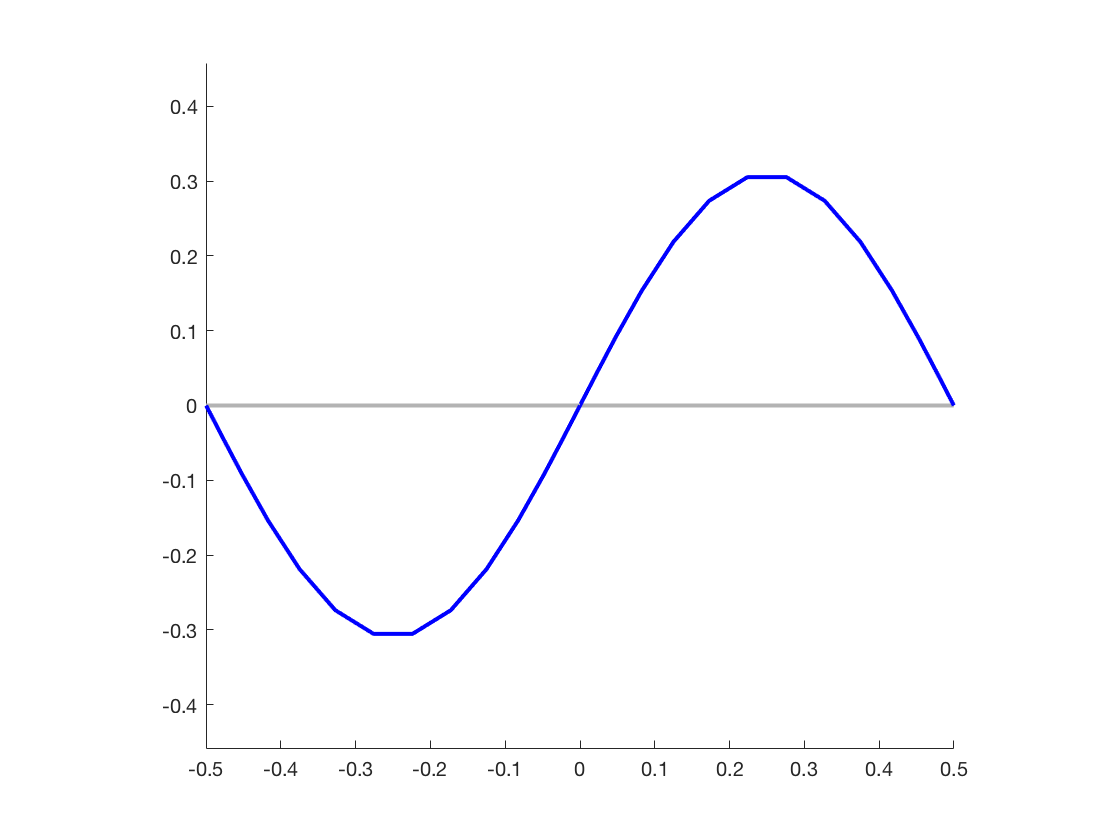
For instance, when $n=2$ we have

	$\displaystyle\big(B_{1,1},B_{2,1}\big)$	$\displaystyle=\left(\tfrac{1}{\sqrt{2}},-\tfrac{1}{\sqrt{2}}\right)$
	$\displaystyle\big(B_{1,2},B_{2,2}\big)$	$\displaystyle=(1,1)$

corresponding to the left and right sides of Figure 1, respectively. Similarly, for $n=3$ we have

	$\displaystyle\big(B_{1,1},B_{2,1},B_{3,1}\big)$	$\displaystyle=\left(\tfrac{1}{2},-1,\tfrac{1}{2}\right)$
	$\displaystyle\big(B_{1,2},B_{2,2},B_{3,2}\big)$	$\displaystyle=\left(\tfrac{\sqrt{3}}{2},0,-\tfrac{\sqrt{3}}{2}\right)$
	$\displaystyle\big(B_{1,3},B_{2,3},B_{3,3}\big)$	$\displaystyle=(1,1,1)$

as shown in Figure 2. In general, we see from (13) that $B_{\cdot,n}=(1,\ldots,1)$ for any value of $n$, consistent with the fact that $u_{n}(x;\sigma)=\sin(n\pi x)$ for all $x\in[0,1]$ and all $\sigma\geq 0$.

To prove the theorem, we first show that the eigenfunctions are given by

(14)

$\displaystyle u_{m}(x;\sigma)=\sin\big(\gamma_m(\sigma)x \big)+\sum_{j=1}^{k-1}A_{j,m}(\sigma)\sin\big(\gamma_m(\sigma)(x- x_j)\big),$

for $x\in[x_{k-1},x_{k}]=\left[\tfrac{k-1}{n},\tfrac{k}{n}\right]$, and with $A_{j,m}(\sigma)$ as in the statement of the theorem. Here we have written $\gamma_{m}(\sigma)=\sqrt{\lambda_{m}(\sigma)}$. The function in (14) clearly satisfies the differential equation

$\displaystyle u_{m}^{\prime\prime}(x;\sigma)=-\lambda_{m}(\sigma)u_{m}(x;\sigma)$

in $(x_{k-1},x_{k})$, and so it remains to check the boundary conditions at $x=0$, $x=1$, and $x=x_{k}$. By construction, $u_{m}(0;\sigma)=0$, and $u_{m}(x;\sigma)$ is continuous at $x=x_{k}$. Therefore, we are left to choose the coefficients $A_{j,m}(\sigma)$ so that $u_{m}(x;\sigma)$ satisfies the Dirichlet condition at the right end-point $x=1$, and the derivative jump conditions at $x=x_{k}$ for each $1\leq k\leq n-1$. The jump in the derivative at $x=x_{k}$ is given by

$\displaystyle u_{m}^{\prime}(x_{k}^{+};\sigma)-u_{m}^{\prime}(x_{k}^{-};\sigma)=A_{k,m}(\sigma)\gamma_{m}(\sigma),$

and $u_{m}(x_{k};\sigma)$ is equal to

$$u_{m}(x_{k};\sigma)=\sin\left(\tfrac{k\gamma_{m}(\sigma)}{n}\right)+A_{1,m}(\sigma)\sin\left(\tfrac{(k-1)\gamma_{m}(\sigma)}{n}\right)+\cdots+A_{k-1,m}(\sigma)\sin\left(\tfrac{\gamma_{m}(\sigma)}{n}\right).$$

Therefore, to ensure that $u_{m}^{\prime}(x_{k}^{+};\sigma)-u_{m}^{\prime}(x_{k}^{-};\sigma)=\sigma u_{m}(x_{k};\sigma)$ and $u_{m}(1;\sigma)=0$, we require $\gamma_{m}(\sigma)$ and $A_{j,m}(\sigma)$ to satisfy

(15)			$\displaystyle A_{k,m}(\sigma)\gamma_{m}(\sigma)=$
		$\displaystyle\hskip 28.45274pt\sigma\left[\sin\left(\tfrac{k\gamma_{m}(\sigma)}{n}\right)+A_{1,m}(\sigma)\sin\left(\tfrac{(k-1)\gamma_{m}(\sigma)}{n}\right)+\cdots+A_{k-1,m}(\sigma)\sin\left(\tfrac{\gamma_{m}(\sigma)}{n}\right)\right]$

for $1\leq k\leq n-1$, and

(16)

$\displaystyle\sin\big(\gamma_m(\sigma) \big)+A_{1,m}(\sigma)\sin\left(\tfrac{(n-1)\gamma_{m}(\sigma)}{n}\right)+\cdots+A_{n-1,m}(\sigma)\sin\left(\tfrac{\gamma_{m}(\sigma)}{n}\right)=0.$

Our strategy to solve the $n-1$ equations (15) and equation (16) is as follows. Using (15) with $k=1$ to solve for $\sigma$, the remaining $n-2$ equations in (15) can be written as

		$\displaystyle A_{k,m}(\sigma)\sin\left(\tfrac{\gamma_{m}(\sigma)}{n}\right)=$
(17)			$\displaystyle\hskip 28.45274ptA_{1,m}(\sigma)\left[\sin\left(\tfrac{k\gamma_{m}(\sigma)}{n}\right)+A_{1,m}(\sigma)\sin\left(\tfrac{(k-1)\gamma_{m}(\sigma)}{n}\right)+\cdots+A_{k-1,m}(\sigma)\sin\left(\tfrac{\gamma_{m}(\sigma)}{n}\right)\right]$

for $2\leq k\leq n-1$. Therefore, for fixed $\sigma$, we first will find the $A_{k,m}(\sigma)$ (in terms of $\gamma_{m}(\sigma)$) that solve (16) and the $n-2$ equations in (17). We finally ensure that (15) holds for $k=1$ by specifying $\gamma_{m}(\sigma)$ in terms of $\sigma$.

Claim: Given $\gamma_{m}(\sigma)$, the coefficients

	$\displaystyle A_{1,m}(\sigma)$	$\displaystyle=2\cos(\theta_m)-2\cos\left(\tfrac{\gamma_{m}(\sigma)}{n}\right),$
	$\displaystyle A_{j,m}(\sigma)$	$\displaystyle=\frac{\sin(j\theta_m)}{\sin(\theta_m)}A_{1,m}(\sigma)\quad\text{ for }2\leq j\leq n-1$

solve the equations (16) and (17) for $2\leq k\leq n-1$. Here $\theta_{m}=\tfrac{m\pi}{n}$.

Proof of Claim: For ease of notation, we omit the dependence on $\sigma$. We will first prove by induction on $k$ that this choice of $A_{j,m}$ satisfies (17) for $2\leq k\leq n-1$. For the base case $k=2$, we have

$\displaystyle A_{2,m}\sin(\gamma_m/n)=\frac{\sin(2\theta_m)}{\sin(\theta_m)}A_{1,m}\sin(\gamma_m/n)=2\cos(\theta_m)A_{1,m}\sin(\gamma_m/n)$

and

		$\displaystyle A_{1,m}\left[\sin(2\gamma_m/n)+A_{1,m}\sin(\gamma_m/n)\right]$
		$\displaystyle=A_{1,m}\left[\sin(2\gamma_m/n)+2\cos(\theta_m)\sin(\gamma_m/n)-2\cos(\gamma_m/n)\sin(\gamma_m/n)\right]$
		$\displaystyle=2A_{1,m}\cos(\theta_m)\sin(\gamma_m/n).$

Therefore, (17) holds for $k=2$. We next assume that (17) holds for $2\leq j\leq k$. Then, using the formula for $A_{1,m}$ we have

		$\displaystyle A_{k,m}\sin(\gamma_m/n)$
		$\displaystyle=A_{1,m}\left[\sin(k\gamma_m/n)+A_{1,m}\sin((k-1)\gamma_m/n)+\cdots+A_{k-1,m}\sin(\gamma_m/n)\right]$
		$\displaystyle=2\cos(\theta_m)\left[\sin(k\gamma_m/n)+A_{1,m}\sin((k-1)\gamma_m/n)+\cdots+A_{k-1,m}\sin(\gamma_m/n)\right]$
		$\displaystyle-2\cos(\gamma_m/n)\left[\sin(k\gamma_m/n)+A_{1,m}\sin((k-1)\gamma_m/n)+\cdots+A_{k-1,m}\sin(\gamma_m/n)\right].$

By the inductive hypothesis (with $j=k$) this implies that

		$\displaystyle A_{k,m}\sin(\gamma_m/n)=2\cos(\theta_m)\frac{A_{k,m}}{A_{1,m}}\sin(\gamma_m/n)$
		$\displaystyle\hskip 28.45274pt-2\cos(\gamma_m/n)\left[\sin(k\gamma_m/n)+A_{1,m}\sin((k-1)\gamma_m/n)+\cdots+A_{k-1,m}\sin(\gamma_m/n)\right].$

Using

$\displaystyle 2\cos(\gamma_m/n)\sin(j\gamma_m/n)=\sin((j+1)\gamma_m/n)+\sin((j-1)\gamma_m/n),$

we can rewrite the above as

		$\displaystyle A_{k,m}\sin(\gamma_m/n)=2\cos(\theta_m)\frac{A_{k,m}}{A_{1,m}}\sin(\gamma_m/n)$
		$\displaystyle\hskip 34.14322pt-\left[\sin((k+1)\gamma_m/n)+A_{1,m}\sin(k\gamma_m/n)+\cdots+A_{k-1,m}\sin(2\gamma_m/n)\right]$
		$\displaystyle\hskip 34.14322pt-\left[\sin((k-1)\gamma_m/n)+A_{1,m}\sin((k-2)\gamma_m/n)+\cdots+A_{k-2,m}\sin(\gamma_m/n)\right].$

Again by the inductive hypothesis (with $j=k-1$), we can rewrite this equation as

	$\displaystyle\sin((k+1)\gamma_m/n)$	$\displaystyle+A_{1,m}\sin(k\gamma_m/n)+\cdots+A_{k-1,m}\sin(2\gamma_m/n)+A_{k,m}\sin(\gamma_m/n)$
(18)			$\displaystyle=2\frac{A_{k,m}}{A_{1,m}}\cos(\theta_m)\sin(\gamma_m/n)-\frac{A_{k-1,m}}{A_{1,m}}\sin(\gamma_m/n).$

Using the formulae for $A_{j,m}/A_{1,m}$ with $j=k-1$ and $j=k$, the right hand side of (18) is equal to

		$\displaystyle\left[2\frac{\sin(k\theta_m)}{\sin(\theta_m)}\cos(\theta_m)-\frac{\sin((k-1)\theta_m)}{\sin(\theta_m)}\cos(\theta_m)\right]\sin(\gamma_m/n)$
		$\displaystyle\qquad=\frac{\sin((k+1)\theta_m)}{\sin(\theta_m)}\sin(\gamma_m/n)=\frac{A_{k+1,m}}{A_{1,m}}\sin(\gamma_m/n).$

This completes the proof of the inductive step, and so (17) holds for all $2\leq k\leq n-1$. To complete the proof of the claim, we finally need to show that the Dirichlet condition in (16) is satisfied. To do this, we apply (18) with $k=n-1$. This gives

	$\displaystyle\sin(\gamma_m)$	$\displaystyle+A_{1,m}\sin((n-1)\gamma_m/n)+\cdots+A_{n-1,m}\sin(\gamma_m/n)$
		$\displaystyle=2\frac{A_{n-1,m}}{A_{1,m}}\cos(\theta_m)\sin(\gamma_m/n)-\frac{A_{n-2,m}}{A_{1,m}}\sin(\gamma_m/n)$
		$\displaystyle=\frac{\sin(n\theta_m)}{\sin(\theta_m)}\sin(\gamma_m/n)=\frac{\sin(m\pi)}{\sin(\theta_m)}\sin(\gamma_m/n)=0$

as required.

To complete the proof of the theorem, we need to find $\gamma_{m}(\sigma)$ in terms of $\sigma$ to ensure that (15) holds for $k=1$, that is

$\displaystyle A_{1,m}(\sigma)\gamma_{m}(\sigma)=\sigma\sin\left(\tfrac{\gamma_{m}(\sigma)}{n}\right).$

Recalling the definition of $A_{1,m}(\sigma)$ and the notation $\gamma_{m}(\sigma)=\sqrt{\lambda_{m}(\sigma)}$, this is precisely the implicit equation for $\lambda_{m}(\sigma)$ given in the statement of the theorem,

(19)

$\displaystyle\sigma=2\gamma_{m}(\sigma)\frac{\cos\left(\tfrac{m\pi}{n}\right)-\cos\big(\tfrac{\gamma_m(\sigma)}{n}\big)}{\sin\big(\tfrac{\gamma_m(\sigma)}{n}\big)}.$

The right-hand side of (19) is a strictly increasing function of $\gamma_{m}(\sigma)$ on the interval $[m\pi,n\pi)$. Moreover, it vanishes when $\gamma_{m}(\sigma)=m\pi$ and becomes unbounded as $\gamma_{m}(\sigma)$ approaches $n\pi$, and hence gives a bijection from $[m\pi,n\pi)$ to $[0,\infty)$. Therefore, for each $\sigma\geq 0$ there is a unique solution $\gamma_{m}(\sigma)$. This solution guarantees that (15) and (16) both hold, and so gives the desired eigenvalue $\lambda_{m}(\sigma)$ and eigenfunction $u_{m}(x;\sigma)$.

References

• [BCM19] Gregory Berkolaiko, Graham Cox, and Jeremy L Marzuola. Nodal deficiency, spectral flow, and the Dirichlet-to-Neumann map. Letters in Mathematical Physics, 109(7):1611–1623, 2019.
• [Ber17] Gregory Berkolaiko. An elementary introduction to quantum graphs. Geometric and computational spectral theory, 700:41–72, 2017.
• [BH16] Pierre Bérard and Bernard Helffer. Courant-sharp eigenvalues for the equilateral torus, and for the equilateral triangle. Letters in Mathematical Physics, 106(12):1729–1789, 2016.
• [BHK20] Pierre Bérard, Bernard Helffer, and Rola Kiwan. Courant-sharp property for Dirichlet eigenfunctions on the Möbius strip. arXiv preprint arXiv:2005.01175, 2020.
• [BKS12] Gregory Berkolaiko, Peter Kuchment, and Uzy Smilansky. Critical partitions and nodal deficiency of billiard eigenfunctions. Geom. Funct. Anal., 22(6):1517–1540, 2012.
• [BNH17] Virginie Bonnaillie-Noël and Bernard Helffer. Nodal and spectral minimal partitions—the state of the art in 2016. In Shape optimization and spectral theory, pages 353–397. De Gruyter Open, Warsaw, 2017.
• [CJM17] Graham Cox, Christoper K. R. T. Jones, and Jeremy L. Marzuola. Manifold decompositions and indices of Schrödinger operators. Indiana Univ. Math. J., 66(5):1573–1602, 2017.
• [DBT08] Tobin A Driscoll, Folkmar Bornemann, and Lloyd N Trefethen. The chebop system for automatic solution of differential equations. BIT Numerical Mathematics, 48(4):701–723, 2008.
• [DH16] Tobin A Driscoll and Nicholas Hale. Rectangular spectral collocation. IMA Journal of Numerical Analysis, 36(1):108–132, 2016.
• [Goo19] Roy H. Goodman. NLS bifurcations on the bowtie combinatorial graph and the dumbbell metric graph. Discrete Contin. Dyn. Syst., 39(4):2203–2232, 2019.
• [HHOT09] Bernard Helffer, Thomas Hoffmann-Ostenhof, and Susanna Terracini. Nodal domains and spectral minimal partitions. In Annales de l’IHP Analyse non linéaire, volume 26, pages 101–138, 2009.
• [HHOT10] Bernard Helffer, Thomas Hoffmann-Ostenhof, and Susanna Terracini. On spectral minimal partitions: the case of the sphere. In Around the Research of Vladimir Maz’ya III, pages 153–178. Springer, 2010.
• [HS16] Bernard Helffer and Mikael Sundqvist. On nodal domains in Euclidean balls. Proceedings of the American Mathematical Society, 144(11):4777–4791, 2016.
• [Lén15] Corentin Léna. Courant-sharp eigenvalues of a two-dimensional torus. Comptes Rendus Mathematique, 353(6):535–539, 2015.
• [Ple56] Åke Pleijel. Remarks on Courant’s nodal line theorem. Comm. Pure Appl. Math., 9:543–550, 1956.
• [XH16] Kuan Xu and Nicholas Hale. Explicit construction of rectangular differentiation matrices. IMA Journal of Numerical Analysis, 36(2):618–632, 2016.