跳到论文正文
W Papers独立论文阅读器 arXiv:2006.13751 论文正文 计算阅读时间 · 0%
引用这篇论文根据当前论文元数据生成,正式投稿前建议核对。


License: arXiv.org perpetual non-exclusive license
arXiv:2006.13751v1 [math.NA] 23 Jun 2020

An adaptive finite element PML method for the open cavity scattering problemsThanks: The research of PL is supported in part by the NSF grant DMS-1912704.

Yanli Chen Address: Department of Mathematics, Northeastern University, Shenyang 110819, China Email address: chenyanli@mail.neu.edu.cn , Peijun Li Address: Department of Mathematics, Purdue University, West Lafayette, Indiana 47907, USA Email address: lipeijun@math.purdue.edu and Xiaokai Yuan Address: School of Mathematical Sciences, Zhejiang University, Hangzhou 310027, China. Email address: yuan170@zju.edu.cn
Abstract.

Consider the electromagnetic scattering of a time-harmonic plane wave by an open cavity which is embedded in a perfectly electrically conducting infinite ground plane. This paper is concerned with the numerical solutions of the transverse electric and magnetic polarizations of the open cavity scattering problems. In each polarization, the scattering problem is reduced equivalently into a boundary value problem of the two-dimensional Helmholtz equation in a bounded domain by using the transparent boundary condition (TBC). An a posteriori estimate based adaptive finite element method with the perfectly matched layer (PML) technique is developed to solve the reduced problem. The estimate takes account both of the finite element approximation error and the PML truncation error, where the latter is shown to decay exponentially with respect to the PML medium parameter and the thickness of the PML layer. Numerical experiments are presented and compared with the adaptive finite element TBC method for both polarizations to illustrate the competitive behavior of the proposed method.

Key words and phrases: 
Electromagnetic cavity scattering, TM and TE polarizations, perfectly matched layer, adaptive finite element method, a posteriori error estimates.

1. Introduction

The phenomena of electromagnetic scattering by open cavities have attracted much attention due to the significant industrial and military applications in such areas as antenna synthesis and stealth design. The underlying scattering problems have been extensively studied by many researchers in the engineering and applied mathematics communities. We refer to the survey [20] and the references cited therein for a comprehensive account on analysis, computation, and optimal design of the cavity scattering problems.

In applications, one of particular interests is the radar cross section (RCS) analysis, which aims at how to mitigate or amplify a signal. The RCS is a quantity which measures the detectability of a target by radar system. Deliberate control in the form of enhancement or reduction of the RCS of a target is of high importance in the electromagnetic interference, especially in the aircraft detection and the stealth design. Since the problems are imposed in open domains and the solutions may have singularities, it presents challenging and significant mathematical and computational questions on precise modeling and accurate computing for the cavity scattering problems in order to successfully implement any desired control of the RCS. This paper concerns the numerical solutions of the open cavity scattering problems. We intend to develop an adaptive finite element method with the perfect matched layer (PML) technique to overcome the difficulties.

The PML technique was first proposed by Bérenger for solving the time-dependent Maxwell equations [7]. Due to its effectiveness, simplicity and flexibility, the PML technique is widely used in computational wave propagation [15, 24, 25, 14]. It has been recognized as one of the most important and popular approaches for the domain truncation. Under the assumption that the exterior solution is composed of outgoing waves only, the basic idea of the PML technique is to surround the domain of interest with a layer of finite thickness of a special medium, which is designed to either slow down or attenuate all the waves propagating into the PML layer from inside of the computational domain. As either the PML parameter or the thickness of the PML layer tends to infinity, the exponential convergence error estimate was obtained in [17, 19] between the solution of the PML problem and the solution of the Helmholtz-type scattering problem. The convergence analysis of the PML problems for the three-dimensional electromagnetic scattering was stuided in [6, 8, 9, 21].

In practice, if we use a very thick PML layer and a uniform finite element mesh, it requires very excessive grids points and hence involves more computational cost. In contrast, if we choose a thin PML layer, it is inevitable to have a rapid variation of the PML medium property, which renders a very fine mesh in order to reach the desired accuracy. On the other hand, the solutions of the open cavity scattering problem may have singularities due to the existence of corners of cavities or the discontinuity of the dielectric coefficient for the filling medium. These singularities slow down the speed of convergence if uniform mesh refinements are applied. The a posteriori error estimate based adaptive finite element method is an ideal tool to handle these issues.

A posteriori error estimators are computable quantities in terms of numerical solutions and data. They measure the error between the numerical solution and the exact solution without requiring any a priori information of the exact solution. A reliable a posteriori error estimator plays a crucial role in an adaptive procedure for mesh modification such as refinement or coarsening. Since the work of Babuška and Rheinboldt [4], the study of adaptive method based on a posteriori error estimator has become an active research topic in scientific computing. Some relevant work can be found in [5, 2, 1, 11, 10] on the adaptive finite element method. We refer to [22, 23, 12, 13] for studies on the scattering problems by using the a posteriori error estimate based adaptive finite element method.

Motivated by the work of Chen and Liu [12], we develop an adaptive procedure, which combines the finite element method and the PML technique, to solve the open cavity scattering problems. Specifically, we consider the electromagnetic scattering of a time-harmonic plane wave by an open cavity embedded in an infinite ground plane. The ground plane and the cavity wall are assumed to be perfect electric conductors. The cavity is assumed to be filled with some inhomogeneous medium, which may protrude out of the cavity to the upper half-space in a finite extend. The upper half-space above the ground plane and the protruding part of the cavity is assumed to be filled with some homogeneous medium. By assuming invariance of the cavity in the x3x_{3} direction, we consider two fundamental polarizations: transverse magnetic (TM) and transverse electric (TE) polarizations, where the three-dimensional Maxwell equations can be reduced to the two-dimensional Helmholtz equation. We restrict our attention to the numerical solutions of the TM and TE polarizations. In each polarization, the scattering problem is reduced equivalently into a boundary value problem of the two-dimensional Helmholtz equation in a bounded domain by using the transparent boundary condition. Computationally, the PML technique is utilized to truncate the infinite half-space above the ground plane and the homogeneous Dirichlet boundary condition is imposed on the outer boundary of the PML layer. The a posteriori error estimate is deduced between the solution of the original scattering problem and the finite element solution of the truncated PML problem. The a posteriori error estimate takes account both of the finite element discretization error and the truncation error of the PML method. The PML truncation error has a nice feature of exponential decay in terms of the PML medium parameter and the thickness of the layer. Based on this property, the proper PML medium parameter and the thickness of the layer can be chosen to make the PML error negligible compared with the finite element discretization error. Once the PML region and the medium property are fixed, the finite element discretization error is used to design the adaptive strategy.

We point out a closely related work [28], where an adaptive finite element method with transparent boundary condition (TBC) was developed for solving the open cavity scattering problems. Since the nonlocal TBC is directly used to truncate the open domain, it does not require a layer of artificially designed absorbing medium to enclose the domain of interest, which makes the TBC method different from the PML approach. But the TBC is given as an infinite series and needs to be truncated into a sum of finitely many terms in computation. Due to the simplicity in the implementation of the PML method, this work provides a viable alternative to the adaptive finite element TBC method for solving the open cavity scattering problems. Numerical experiments are presented and compared with the adaptive finite element TBC method for both polarizations to illustrate the competitive behavior of the adaptive finite element PML method.

The outline of this paper is as follows. In Section 2, we introduce the problem formulation, where the governing equations are given for the TM and TE polarizations. Sections 3 and 4 are devoted to the analysis of the TM and TE polarizations, respectively. Topics are organized to address the variational problem, the PML problem and its convergence, the finite element approximation, the a posteriori error analysis for the discrete truncated PML problem, and the adaptive finite element algorithm. In Section 5, some numerical examples are presented to illustrate the performance of the proposed method. The paper is concluded with some general remarks in Section 6.

2. Problem formulation

Let us first specify the problem geometry which is shown in Figure 1. Denote by D⊂ℝ2D\subset\mathbb{R}^{2} the cross section of an x3x_{3}-invariant cavity with a Lipschitz continuous boundary ∂D=S∪Γ\partial D=S\cup\Gamma, where SS refers to as the cavity wall and Γ\Gamma is the opening of the cavity. We assume that the cavity wall SS is a perfect electric conductor and the opening Γ\Gamma is aligned with the perfectly electrically conducting infinite ground plane Γg\Gamma_{g}. The cavity may be filled with some inhomogeneous medium, which can be characterized by the dielectric permittivity ϵ\epsilon and the magnetic permeability μ\mu. Moreover, the medium may protrude from the cavity into the upper half-space. In this case, the cavity is called an overfilled cavity. Let BR+B_{R}^{+} and Bρ+B_{\rho}^{+} be the upper half-discs with radii RR and ρ\rho, where ρ>R>0\rho>R>0. Denote by ΓR+\Gamma_{R}^{+} and Γρ+\Gamma_{\rho}^{+} the upper semi-circles. The radius RR can be chosen large enough such that the upper half-disc BR+B_{R}^{+} can enclose the possibly protruding inhomogeneous medium from the cavity. The infinite exterior domain ℝ2∖BR+¯\mathbb{R}^{2}\setminus\overline{B_{R}^{+}} is assumed to be filled with some homogeneous medium with a constant dielectric permittivity ϵ0\epsilon_{0} and a constant magnetic permeability μ0\mu_{0}.

Refer to caption
Figure 1. Schematic of the open cavity scattering problem.

Since the structure is invariant the x3x_{3}-axis, we consider two fundamental polarizations: transverse magnetic (TM) polarization and transverse electric (TE) polarization. The three-dimensional Maxwell equations can be reduced to the two-dimensional Helmholtz equation under these two modes. In the TM polarization, the magnetic field is transverse to the x3x_{3}-axis and the electric field has the form 𝑬⁡(x1,x2)=(0,0,u⁡(x1,x2))⊤\boldsymbol{E}(x_{1},x_{2})=(0,0,u(x_{1},x_{2}))^{\top}, where the scalar function uu satisfies

{Δ​u+κ2​u=0in​ℝ+2∪D,u=0on​Γg∪S,\begin{cases}\Delta u+\kappa^{2}u=0&\quad\text{in}~\mathbb{R}^{2}_{+}\cup D,\\ u=0&\quad\text{on}~\Gamma_{g}\cup S,\end{cases} (2.1)

where κ=ω​(ε​μ)1/2\kappa=\omega(\varepsilon\mu)^{1/2} is the wave number and ω>0\omega>0 is the angular frequency. In the TE polarization, the electric field is transverse to the x3x_{3}-axis and the magnetic field takes the form 𝑯⁡(x1,x2)=(0,0,u⁡(x1,x2))⊤\boldsymbol{H}(x_{1},x_{2})=(0,0,u(x_{1},x_{2}))^{\top}, where uu satisfies

{∇⋅(κ−2∇u)+u=0in​ℝ+2∪D,∂νu=0on​Γg∪S,\begin{cases}\nabla\cdot(\kappa^{-2}\nabla u)+u=0&\quad\text{in}~\mathbb{R}^{2}_{+}\cup D,\\ \partial_{\nu}u=0&\quad\text{on}~\Gamma_{g}\cup S,\end{cases} (2.2)

where ν\nu is the unit outward normal vector to Γg∪S\Gamma_{g}\cup S.

Consider the incidence of a plane wave

ui​(x1,x2)=ei⁡(k1​x1−k2​x2),u^{\rm i}(x_{1},x_{2})=e^{i(k_{1}x_{1}-k_{2}x_{2})},

which is sent from the above to impinge the cavity. Here k1=κ0sinθ,k2=κ0cosθ,θ∈(−π/2,π/2)k_{1}=\kappa_{0}\sin\theta,k_{2}=\kappa_{0}\cos\theta,\theta\in(-\pi/2,\pi/2) is the angle of the incidence, and κ0=ω​(ε0​μ0)1/2\kappa_{0}=\omega(\varepsilon_{0}\mu_{0})^{1/2} is the wavenumber in the free space. Due to the perfectly electrically conducting ground plane, the reflected field in the TM polarization is

ur​(x1,x2)=−ei⁡(k1​x1+k2​x2),u^{\rm r}(x_{1},x_{2})=-e^{i(k_{1}x_{1}+k_{2}x_{2})},

while the reflected field in the TE polarization is

ur​(x1,x2)=ei⁡(k1​x1+k2​x2).u^{\rm r}(x_{1},x_{2})=e^{i(k_{1}x_{1}+k_{2}x_{2})}.

Let the reference field urefu^{\rm ref} be the superposition of the incident field and the reflected field, i.e., uref=ui+uru^{\rm ref}=u^{\rm i}+u^{\rm r}. The total field uu consists of the reference field urefu^{\rm ref} and the scattered field usu^{\rm s}, i.e.,

u=uref+us.u=u^{\rm ref}+u^{\rm s}.

In addition, the scattered field usu^{\rm s} is required to satisfy the Sommerfeld radiation condition

limr=|x|→∞r1/2​(∂rus−i​κ0​us)=0.\lim_{r=|x|\rightarrow\infty}r^{1/2}(\partial_{r}u^{\rm s}-i\kappa_{0}u^{\rm s})=0. (2.3)

3. TM polarization

In this section, we consider the TM polarization. First the transparent boundary condition is introduced to reduce the open cavity problem into a boundary value problem in a bounded domain. Next the variational problem is described, and the PML problem and its convergence are discussed. Then the finite element approximation and the a posteriori error estimate are studied. Finally the adaptive finite element method with PML is presented for solving the discrete PML problem.

3.1. The variational problem

It can be verified from (2.1) that the scattered field usu^{\rm s} satisfies the Helmholtz equation

Δ​us+κ02​us=0in​ℝ+2∖BR+¯.\Delta u^{\rm s}+\kappa_{0}^{2}u^{\rm s}=0\qquad\mathrm{in}~\mathbb{R}^{2}_{+}\setminus\overline{B_{R}^{+}}. (3.1)

Based on the radiation condition (2.3), we know that the solution of (3.1) has the Fourier series expansion

us​(r,ϕ)=∑n=0∞Hn(1)​(κ0​r)Hn(1)​(κ0​R)​(an​sin⁡(n​ϕ)+bn​cos⁡(n​ϕ)),r≥R,u^{\rm s}(r,\phi)=\sum_{n=0}^{\infty}\frac{H_{n}^{(1)}(\kappa_{0}r)}{H_{n}^{(1)}(\kappa_{0}R)}(a_{n}\sin(n\phi)+b_{n}\cos(n\phi)),\quad r\geq R, (3.2)

where Hn(1)H_{n}^{(1)} is the Hankel function of the first kind with order nn. Noting the fact u=0u=0 and uref=0u^{\rm ref}=0 on Γg\Gamma_{g}, we have us​(r,0)=us​(r,π)=0u^{\rm s}(r,0)=u^{\rm s}(r,\pi)=0, which implies bn=0b_{n}=0 and (3.2) reduces to

us​(r,ϕ)=∑n=1∞Hn(1)​(κ0​r)Hn(1)​(κ0​R)​an​sin⁡(n​ϕ),r≥R.u^{\rm s}(r,\phi)=\sum_{n=1}^{\infty}\frac{H_{n}^{(1)}(\kappa_{0}r)}{H_{n}^{(1)}(\kappa_{0}R)}a_{n}\sin(n\phi),\quad r\geq R. (3.3)

Taking the partial derivative of (3.3) with respect to rr and evaluating it at r=Rr=R yields

∂rus​(R,ϕ)=κ0​∑n=1∞Hn(1)′​(κ0​R)Hn(1)​(κ0​R)​an​sin⁡(n​ϕ).\partial_{r}u^{\rm s}(R,\phi)=\kappa_{0}\sum_{n=1}^{\infty}\frac{{H_{n}^{(1)^{\prime}}}(\kappa_{0}R)}{H_{n}^{(1)}(\kappa_{0}R)}a_{n}\sin(n\phi). (3.4)

Let LTM2​(ΓR+):={u∈L2​(ΓR+):u⁡(R,0)=u⁡(R,π)=0}L^{2}_{\rm TM}(\Gamma_{R}^{+}):=\{u\in L^{2}(\Gamma_{R}^{+}):u(R,0)=u(R,\pi)=0\}. For any u∈LTM2​(ΓR+)u\in L^{2}_{\rm TM}(\Gamma_{R}^{+}), it has the Fourier series expansion

u⁡(R,ϕ)=∑n=1∞an​sin⁡(n​ϕ),an=2π​∫0πu⁡(R,ϕ)​sin⁡(n​ϕ)​𝑑ϕ.u(R,\phi)=\sum_{n=1}^{\infty}a_{n}\sin(n\phi),\quad a_{n}=\frac{2}{\pi}\int_{0}^{\pi}u(R,\phi)\sin(n\phi){\rm d}\phi.

Define the trace function space HTMs​(ΓR+):={u∈LTM2​(ΓR+):‖u‖HTMs​(ΓR+)≤∞}H^{s}_{\rm TM}(\Gamma_{R}^{+}):=\{u\in L^{2}_{\rm TM}(\Gamma_{R}^{+}):\|u\|_{H^{s}_{\rm TM}(\Gamma_{R}^{+})}\leq\infty\}, where the HTMs​(ΓR+)H^{s}_{\rm TM}(\Gamma_{R}^{+}) norm is given by

‖u‖HTMs​(ΓR+)=(∑n=1∞(1+n2)s​|an|2)1/2.\|u\|_{H^{s}_{\rm TM}(\Gamma_{R}^{+})}=\left(\sum_{n=1}^{\infty}(1+n^{2})^{s}|a_{n}|^{2}\right)^{1/2}.

It is clear that the dual space of HTMs​(ΓR+)H^{s}_{\rm TM}(\Gamma_{R}^{+}) is HTM−s​(ΓR+)H^{-s}_{\rm TM}(\Gamma_{R}^{+}) with respect to the scalar product in L2​(ΓR+)L^{2}(\Gamma_{R}^{+}) given by

⟨u,v⟩ΓR+=∫ΓR+u​v¯​𝑑s.\langle u,v\rangle_{\Gamma_{R}^{+}}=\int_{\Gamma_{R}^{+}}u\bar{v}{\rm d}s.

Introduce the DtN operator

(ℬTM​u)​(R,ϕ)=κ0​∑n=1∞Hn(1)′​(κ0​R)Hn(1)​(κ0​R)​an​sin⁡(n​ϕ)on​ΓR+.(\mathscr{B}_{\rm TM}u)(R,\phi)=\kappa_{0}\sum_{n=1}^{\infty}\frac{{H_{n}^{(1)^{\prime}}}(\kappa_{0}R)}{H_{n}^{(1)}(\kappa_{0}R)}a_{n}\sin(n\phi)\quad\text{on}~\Gamma_{R}^{+}. (3.5)

It is shown in [27] that the boundary operator ℬTM:HTM1/2(ΓR+)→HTM−1/2(ΓR+)\mathscr{B}_{\rm TM}:H^{1/2}_{\rm TM}(\Gamma_{R}^{+})\rightarrow H^{-1/2}_{\rm TM}(\Gamma_{R}^{+}) is continuous. Using (3.4)–(3.5), we obtain the transparent boundary condition for the scattered field usu^{\rm s}:

∂rus=ℬTM​uson​ΓR+,\partial_{r}u^{\rm s}=\mathscr{B}_{\rm TM}u^{\rm s}\quad{\rm on}~\Gamma_{R}^{+},

which can be equivalently imposed for the total field uu:

∂ru=ℬTM​u+fon​ΓR+,\partial_{r}u=\mathscr{B}_{\rm TM}u+f\quad{\rm on}~\Gamma_{R}^{+},

where f=∂ruref−ℬTM​ureff=\partial_{r}u^{\rm ref}-\mathscr{B}_{\rm TM}u^{\rm ref}.

Let Ω=BR+∪D\Omega=B_{R}^{+}\cup D. The open cavity scattering problem can be reduced to the following boundary value problem:

{Δ​u+κ2​u=0in​Ω,u=0on​Γg∪S,∂ru=ℬTM​u+fon​ΓR+,\begin{cases}\Delta u+\kappa^{2}u=0&\quad\text{in}~\Omega,\\ u=0&\quad\text{on}~\Gamma_{g}\cup S,\\ \partial_{r}u=\mathscr{B}_{\rm TM}u+f&\quad\text{on}~\Gamma_{R}^{+},\end{cases}

which has the variational formulation: find u∈HS1​(Ω)={u∈H1​(Ω):u=0​on​Γg∪S}u\in H_{S}^{1}(\Omega)=\{u\in H^{1}(\Omega):u=0~\text{on}~\Gamma_{g}\cup S\} such that

aTM​(u,v)=⟨f,v⟩ΓR+∀v∈HS1​(Ω),a_{\rm TM}(u,v)=\langle f,v\rangle_{\Gamma_{R}^{+}}\quad\forall\,v\in H_{S}^{1}(\Omega), (3.6)

where the sesquilinear form aTM​(⋅,⋅):H1​(Ω)×H1​(Ω)→ℂa_{\rm TM}(\cdot,\cdot):H^{1}(\Omega)\times H^{1}(\Omega)\to\mathbb{C} is defined by

aTM​(u,v)=∫Ω(∇u⋅∇v¯−κ2​u​v¯)​𝑑x−⟨ℬTM​u,v⟩ΓR+.a_{\rm TM}(u,v)=\int_{\Omega}\left(\nabla u\cdot\nabla\bar{v}-\kappa^{2}u\bar{v}\right){\rm d}x-\langle\mathscr{B}_{\rm TM}u,v\rangle_{\Gamma_{R}^{+}}. (3.7)

The following result states the well-posedness of the variational problem (3.6). The proof can be found in [27].

Theorem 3.1.

The variational problem (3.6) has a unique weak solution in HS1​(Ω)H_{S}^{1}(\Omega), which satisfies the estimate

∥u∥H1​(Ω)≤C∥f∥H−1/2TM(ΓR+),\|u\|_{H^{1}(\Omega)}\leq C\|f\|_{H^{-1/2}_{\rm TM}(\Gamma_{R}^{+})},

where C>0C>0 is a constant.

It follows from the general theory in Babusˇ\check{\rm s}ka and Aziz [3, Chapter 5] that there exists a constant C>0C>0 such that the following inf-sup condition holds:

sup0≠v∈HS1​(Ω)|aTM​(u,v)|‖v‖H1​(Ω)≥C​‖u‖H1​(Ω)∀u∈HS1​(Ω).\sup\limits_{0\neq v\in H_{S}^{1}(\Omega)}\frac{|a_{\rm TM}(u,v)|}{\|v\|_{H^{1}(\Omega)}}\geq C\|u\|_{H^{1}(\Omega)}\quad\forall\,u\in H_{S}^{1}(\Omega). (3.8)

3.2. The PML problem

Let ΩPML={x∈ℝ+2:R<|x|<ρ}\Omega^{\rm PML}=\{x\in\mathbb{R}^{2}_{+}:R<|x|<\rho\} be the PML region which encloses the bounded domain Ω\Omega in the upper half-space. Denote by Ωρ=Bρ+∪D\Omega_{\rho}=B_{\rho}^{+}\cup D the computational domain in which the truncated PML problem is formulated.

Define the PML parameters by using the complex coordinate stretching

r~=∫0rα⁡(t)​𝑑t=r​β​(r),\tilde{r}=\int_{0}^{r}\alpha(t){\rm d}t=r\beta(r), (3.9)

where α⁡(r)=1+i​σ​(r)\alpha(r)=1+i\sigma(r). In practice, σ\sigma is usually taken as a power function

σ⁡(r)={0,0≤r<R,σ0​(r−Rρ−R)m,r≥R,\sigma(r)=\begin{cases}0,&0\leq r<R,\\ \sigma_{0}\big(\frac{r-R}{\rho-R}\big)^{m},&r\geq R,\end{cases}

where σ0\sigma_{0} is a positive constant and m≥1m\geq 1 is an integer. It can be seen from (3.9) that

β⁡(r)=1+i​σ^​(r),σ^​(r)=1r​∫Rrσ⁡(t)​𝑑t.\beta(r)=1+i\hat{\sigma}(r),\quad\hat{\sigma}(r)=\frac{1}{r}\int_{R}^{r}\sigma(t){\rm d}t.

In the polar coordinates, the gradient and divergence operators can be written as

∇u=∂ru​𝒆r+1r​∂ϕu​𝒆ϕ,∇⋅𝒖=1r​∂r(r​ur)+1r​∂ϕuϕ,\displaystyle\nabla u=\partial_{r}u\boldsymbol{e}_{r}+\frac{1}{r}\partial_{\phi}u\boldsymbol{e}_{\phi},\quad\nabla\cdot\boldsymbol{u}=\frac{1}{r}\partial_{r}(ru_{r})+\frac{1}{r}\partial_{\phi}u_{\phi}, (3.10)

where 𝒖=ur​𝒆r+uϕ​𝒆ϕ\boldsymbol{u}=u_{r}\boldsymbol{e}_{r}+u_{\phi}\boldsymbol{e}_{\phi} and 𝒆r=(cos⁡ϕ,sin⁡ϕ)⊤,𝒆ϕ=(−sin⁡ϕ,cos⁡ϕ)⊤\boldsymbol{e}_{r}=(\cos\phi,\sin\phi)^{\top},\boldsymbol{e}_{\phi}=(-\sin\phi,\cos\phi)^{\top}. By the chain rule and (3.9), a simple calculation yields

∂r~u=∂ru⁡(d​rd​r~)=1α⁡(r)​∂ru.\partial_{\tilde{r}}u=\partial_{r}u\left(\frac{{\rm d}r}{{\rm d}\tilde{r}}\right)=\frac{1}{\alpha(r)}\partial_{r}u. (3.11)

Combining (3.10) and (3.11), we introduce the modified gradient operator

∇~​u=1α⁡(r)​∂ru​𝒆r+1r​β​(r)​∂ϕu​𝒆ϕ.\tilde{\nabla}u=\frac{1}{\alpha(r)}\partial_{r}u\boldsymbol{e}_{r}+\frac{1}{r\beta(r)}\partial_{\phi}u\boldsymbol{e}_{\phi}.

It is easy to verify

Δ~u=1r​α​(r)​β​(r)∂r(r​β​(r)α⁡(r)∂ru)+1r​β​(r)∂ϕ(1r​β​(r)∂ϕu)=1α​β∇⋅(A∇u),\displaystyle\tilde{\Delta}u=\frac{1}{r\alpha(r)\beta(r)}\partial_{r}\left(\frac{r\beta(r)}{\alpha(r)}\partial_{r}u\right)+\frac{1}{r\beta(r)}\partial_{\phi}\left(\frac{1}{r\beta(r)}\partial_{\phi}u\right)=\frac{1}{\alpha\beta}\nabla\cdot(A\nabla u),

where

A=[β⁡(r)α⁡(r)​cos2⁡ϕ+α⁡(r)β⁡(r)​sin2⁡ϕ(β⁡(r)α⁡(r)−α⁡(r)β⁡(r))​sin⁡ϕ​cos⁡ϕ(β⁡(r)α⁡(r)−α⁡(r)β⁡(r))​sin⁡ϕ​cos⁡ϕβ⁡(r)α⁡(r)​sin2⁡ϕ+α⁡(r)β⁡(r)​cos2⁡ϕ].A=\begin{bmatrix}\frac{\beta(r)}{\alpha(r)}\cos^{2}\phi+\frac{\alpha(r)}{\beta(r)}\sin^{2}\phi&\left(\frac{\beta(r)}{\alpha(r)}-\frac{\alpha(r)}{\beta(r)}\right)\sin\phi\cos\phi\\ \left(\frac{\beta(r)}{\alpha(r)}-\frac{\alpha(r)}{\beta(r)}\right)\sin\phi\cos\phi&\frac{\beta(r)}{\alpha(r)}\sin^{2}\phi+\frac{\alpha(r)}{\beta(r)}\cos^{2}\phi\end{bmatrix}.

Hence we obtain the PML equation for the scattered field us,PMLu^{\rm s,PML}:

∇⋅(A∇us,PML)+κ02αβus,PML=0inℝ+2∖BR+¯,\nabla\cdot(A\nabla u^{\rm s,PML})+\kappa_{0}^{2}\alpha\beta u^{\rm s,PML}=0\quad\text{in}~\mathbb{R}^{2}_{+}\setminus\overline{B_{R}^{+}},

where us,PMLu^{\rm s,PML} is required to be uniformly bounded as r=|x|→∞r=|x|\to\infty. In practice, the open domain ℝ+2∖BR+¯\mathbb{R}^{2}_{+}\setminus\overline{B_{R}^{+}} needs to be truncated into a bounded domain. Replacing rr with r~\tilde{r} in (3.3) and noting the exponential decay of the Hankel functions with a complex argument, we can observe that the scattered field us,PMLu^{\rm s,PML} decays exponentially in ℝ+2∖BR+¯\mathbb{R}^{2}_{+}\setminus\overline{B_{R}^{+}}. Hence it is reasonable to impose the Dirichlet boundary condition

us,PML=0on​Γρ+.u^{\rm s,PML}=0\quad{\rm on}~\Gamma_{\rho}^{+}.

We obtain the truncated PML problem

{∇⋅(A∇uPML)+κ2αβuPML=Fin​Ωρ,uPML=0on​Γg∪S,uPML=urefon​Γρ+,\begin{cases}\nabla\cdot(A\nabla u^{\rm PML})+\kappa^{2}\alpha\beta u^{\rm PML}=F&\quad\text{in}~\Omega_{\rho},\\ u^{\rm PML}=0&\quad\text{on}~\Gamma_{g}\cup S,\\ u^{\rm PML}=u^{\rm ref}&\quad\text{on}~\Gamma_{\rho}^{+},\end{cases} (3.12)

where

F={∇⋅(A∇uref)+κ02αβurefin​ΩPML,0otherwise.F=\begin{cases}\nabla\cdot(A\nabla u^{\rm ref})+\kappa_{0}^{2}\alpha\beta u^{\rm ref}&\mathrm{in}~\Omega^{\rm PML},\\ 0&{\rm otherwise}.\end{cases}

Introduce another DtN operator ℬ^TM:HTM1/2(ΓR+)→HTM−1/2(ΓR+)\hat{\mathscr{B}}_{\rm TM}:H^{1/2}_{\rm TM}(\Gamma_{R}^{+})\rightarrow H^{-1/2}_{\rm TM}(\Gamma_{R}^{+}) which defined as follows: given ζ∈HTM1/2​(ΓR+)\zeta\in H^{1/2}_{\rm TM}(\Gamma_{R}^{+}),

ℬ^TM​ζ=∂rξ|ΓR+,\hat{\mathscr{B}}_{\rm TM}\zeta=\partial_{r}\xi|_{\Gamma_{R}^{+}},

where ξ∈H1​(ΩPML)\xi\in H^{1}(\Omega^{\rm PML}) satisfies

{∇⋅(A∇ξ)+κ2αβξ=0in​ΩPML,ξ=ζon​ΓR+,ξ=0on​Γg∪Γρ+.\begin{cases}\nabla\cdot(A\nabla\xi)+\kappa^{2}\alpha\beta\xi=0&\quad\text{in}~\Omega^{\rm PML},\\ \xi=\zeta&\quad\text{on}~\Gamma_{R}^{+},\\ \xi=0&\quad\text{on}~\Gamma_{g}\cup\Gamma_{\rho}^{+}.\end{cases}

Using the boundary condition

∂r(uPML−uref)|ΓR+=ℬ^TM​(uPML−uref),\partial_{r}(u^{\rm PML}-u^{\rm ref})|_{\Gamma_{R}^{+}}=\hat{\mathscr{B}}_{\rm TM}(u^{\rm PML}-u^{\rm ref}),

and noting A=I,α=β=1A=I,\alpha=\beta=1 in Ω\Omega, we reformulate (3.12) equivalently into the following boundary value problem:

{Δ​uPML+κ2​uPML=0in​Ω,uPML=0on​Γg∪S,∂ruPML=ℬ^TM​uPML+f^on​ΓR+,\begin{cases}\Delta u^{\rm PML}+\kappa^{2}u^{\rm PML}=0&\quad\mathrm{in}~\Omega,\\ u^{\rm PML}=0&\quad\mathrm{on}~\Gamma_{g}\cup S,\\ \partial_{r}u^{\rm PML}=\hat{\mathscr{B}}_{\rm TM}u^{\rm PML}+\hat{f}&\quad{\rm on}~\Gamma_{R}^{+},\end{cases} (3.13)

where f^=∂ruref−ℬ^TM​uref\hat{f}=\partial_{r}u^{\rm ref}-\hat{\mathscr{B}}_{\rm TM}u^{\rm ref}. The weak formulation of the problem (3.13) is to find uPML∈HS1​(Ω)u^{\rm PML}\in H_{S}^{1}(\Omega) such that

a^TM​(uPML,v)=⟨f^,v⟩ΓR+∀v∈HS1​(Ω),\hat{a}_{\rm TM}(u^{\rm PML},v)=\langle\hat{f},v\rangle_{\Gamma_{R}^{+}}\quad\forall\,v\in H_{S}^{1}(\Omega), (3.14)

where the sesquilinear form a^TM​(⋅,⋅):H1​(Ω)×H1​(Ω)→ℂ\hat{a}_{\rm TM}(\cdot,\cdot):H^{1}(\Omega)\times H^{1}(\Omega)\rightarrow\mathbb{C} is defined as

a^TM​(u,v)=∫Ω(∇u⋅∇v¯−κ2​u​v¯)​𝑑x−⟨ℬ^TM​u,v⟩ΓR+.\hat{a}_{\rm TM}(u,v)=\int_{\Omega}\left(\nabla u\cdot\nabla\bar{v}-\kappa^{2}u\bar{v}\right){\rm d}x-\langle\hat{\mathscr{B}}_{\rm TM}u,v\rangle_{\Gamma_{R}^{+}}.

3.3. Convergence of the PML problem

Consider a boundary value problem of the PML equation in ΩPML\Omega^{\rm PML}:

{∇⋅(A∇w)+κ02αβw=0in​ΩPML,w=0on​Γg∪ΓR+,w=qon​Γρ+.\begin{cases}\nabla\cdot(A\nabla w)+\kappa_{0}^{2}\alpha\beta w=0&\quad\mathrm{in}~\Omega^{\rm PML},\\ w=0&\quad\mathrm{on}~\Gamma_{g}\cup\Gamma_{R}^{+},\\ w=q&\quad{\rm on}~\Gamma_{\rho}^{+}.\end{cases} (3.15)

Define H01​(ΩPML)={u∈H1​(ΩPML):u=0​on​Γg∪ΓR+∪Γρ+}H^{1}_{0}(\Omega^{\rm PML})=\{u\in H^{1}(\Omega^{\rm PML}):u=0~\text{on}~\Gamma_{g}\cup\Gamma_{R}^{+}\cup\Gamma_{\rho}^{+}\}. Given q∈HTM1/2​(Γρ+)q\in H^{1/2}_{\rm TM}(\Gamma_{\rho}^{+}), the weak formulation of (3.15) is to find w∈H1​(ΩPML)w\in H^{1}(\Omega^{\rm PML}) such that w=0​on​Γg∪ΓR+,w=q​on​Γρ+w=0~{\rm on}~\Gamma_{g}\cup\Gamma_{R}^{+},w=q~{\rm on}~\Gamma_{\rho}^{+} and

b^​(w,v)=0∀v∈H01​(ΩPML),\hat{b}(w,v)=0\quad\forall\,v\in H^{1}_{0}(\Omega^{\rm PML}), (3.16)

where the sesquilinear form b^​(⋅,⋅):H1​(ΩPML)×H1​(ΩPML)→ℂ\hat{b}(\cdot,\cdot):H^{1}(\Omega^{\rm PML})\times H^{1}(\Omega^{\rm PML})\to\mathbb{C} is

b^​(u,v)=∫Rρ∫0π(β​rα​∂ru​∂rv¯+αβ​r​∂ϕu​∂ϕv¯−κ02​α​β​r​u​v¯)​𝑑r​𝑑ϕ.\hat{b}(u,v)=\int_{R}^{\rho}\int_{0}^{\pi}\left(\frac{\beta r}{\alpha}\partial_{r}u\partial_{r}\bar{v}+\frac{\alpha}{\beta r}\partial_{\phi}u\partial_{\phi}\bar{v}-\kappa_{0}^{2}\alpha\beta ru\bar{v}\right){\rm d}r{\rm d}\phi.

As is discussed in [16], in general, the uniqueness of (3.16) can not be guaranteed due to the possible existence of eigenvalues which form a discrete set. Since our focus is on the convergence analysis, we simply assume that the PML problem (3.16) has a unique solution in the PML region.

For any u∈H1​(ΩPML)u\in H^{1}(\Omega^{\rm PML}), define

‖u‖∗,ΩPML=[∫Rρ∫0π((1+σ​σ^1+σ2)​r​|∂ru|2+(1+σ​σ^1+σ^2)​1r​|∂ϕu|2+(1+σ​σ^)​κ02​r​|u|2)​𝑑r​𝑑ϕ]1/2.\|u\|_{\ast,\Omega^{\rm PML}}=\left[\int_{R}^{\rho}\int_{0}^{\pi}\left(\Big(\frac{1+\sigma\hat{\sigma}}{1+\sigma^{2}}\Big)r|\partial_{r}u|^{2}+\bigg(\frac{1+\sigma\hat{\sigma}}{1+\hat{\sigma}^{2}}\bigg)\frac{1}{r}|\partial_{\phi}u|^{2}+(1+\sigma\hat{\sigma})\kappa_{0}^{2}r|u|^{2}\right){\rm d}r{\rm d}\phi\right]^{1/2}.

It is easy to show that the norm ∥⋅∥∗,ΩPML\|\cdot\|_{\ast,\Omega^{\rm PML}} is equivalent to the usual H1​(ΩPML)H^{1}(\Omega^{\rm PML})-norm. An application of the general theory in [3, Chapter 5] implies that there exists a positive constant C^\hat{C} depending on ΩPML\Omega^{\rm PML} and κ0\kappa_{0} such that

sup0≠v∈H01​(ΩPML)|b^​(u,v)|‖v‖∗,ΩPML≥C^​‖u‖∗,ΩPML∀u∈H01​(ΩPML).\sup_{0\neq v\in H^{1}_{0}(\Omega^{\rm PML})}\frac{|\hat{b}(u,v)|}{\|v\|_{\ast,\Omega^{\rm PML}}}\geq\hat{C}\|u\|_{\ast,\Omega^{\rm PML}}\quad\forall\,u\in H^{1}_{0}(\Omega^{\rm PML}). (3.17)

The following results play an important role in the convergence analysis. The proof is similar to that of [12, Theorem 2.4] for solving the obstacle scattering problem and is omitted here for brevity.

Theorem 3.2.

There exists a constant C>0C>0 independent of κ0,R,ρ\kappa_{0},R,\rho, and σ0\sigma_{0} such that the following estimates are satisfied:

∥|α|−1∇w∥L2​(ΩPML)\displaystyle\||\alpha|^{-1}\nabla w\|_{L^{2}(\Omega^{\rm PML})} ≤\displaystyle\leq C​C^−1​(1+κ0​R)​|α0|​‖q‖HTM1/2​(Γρ+),\displaystyle C\hat{C}^{-1}(1+\kappa_{0}R)|\alpha_{0}|\|q\|_{H^{1/2}_{\rm TM}(\Gamma_{\rho}^{+})}, (3.18)
‖∂rw‖H−1/2TM(ΓR+)\displaystyle\left\|\partial_{r}w\right\|_{H^{-1/2}_{\rm TM}(\Gamma_{R}^{+})} ≤\displaystyle\leq C​C^−1​(1+κ0​R)2​|α0|2​‖q‖HTM1/2​(Γρ+),\displaystyle C\hat{C}^{-1}(1+\kappa_{0}R)^{2}|\alpha_{0}|^{2}\|q\|_{H^{1/2}_{\rm TM}(\Gamma_{\rho}^{+})}, (3.19)

where C^\hat{C} is given in (3.17) and α0=1+i​σ0\alpha_{0}=1+i\sigma_{0}.

Following the idea in [19], for any function f∈HTM1/2​(ΓR+)f\in H^{1/2}_{\rm TM}(\Gamma_{R}^{+}), we introduce the propagation operator 𝒫TM:HTM1/2​(ΓR+)→HTM1/2​(Γρ+)\mathscr{P}_{\rm TM}:H^{1/2}_{\rm TM}(\Gamma_{R}^{+})\rightarrow H^{1/2}_{\rm TM}(\Gamma_{\rho}^{+}) defined by

𝒫TM​(f)=∑n=1∞Hn(1)​(κ0​ρ~)Hn(1)​(κ0​R)​fn​sin⁡(n​ϕ),fn=2π​∫0πf⁡(R,ϕ)​sin⁡(n​ϕ)​𝑑ϕ.\mathscr{P}_{\rm TM}(f)=\sum_{n=1}^{\infty}\frac{H_{n}^{(1)}(\kappa_{0}\tilde{\rho})}{H_{n}^{(1)}(\kappa_{0}R)}f_{n}\sin(n\phi),\quad f_{n}=\frac{2}{\pi}\int_{0}^{\pi}f(R,\phi)\sin(n\phi){\rm d}\phi.

As shown in [12], the operator 𝒫TM:HTM1/2​(ΓR+)→HTM1/2​(Γρ+)\mathscr{P}_{\rm TM}:H^{1/2}_{\rm TM}(\Gamma_{R}^{+})\rightarrow H^{1/2}_{\rm TM}(\Gamma_{\rho}^{+}) is well defined and satisfies the estimate

‖𝒫TM​(f)‖HTM1/2​(Γρ+)≤e−κ0​ℑ⁡(ρ~)​(1−R2|ρ~|2)1/2​‖f‖HTM1/2​(ΓR+)∀ρ≥R.\|\mathscr{P}_{\rm TM}(f)\|_{H^{1/2}_{\rm TM}(\Gamma_{\rho}^{+})}\leq e^{-\kappa_{0}\Im(\tilde{\rho})\left(1-\frac{R^{2}}{|\tilde{\rho}|^{2}}\right)^{1/2}}\|f\|_{H^{1/2}_{\rm TM}(\Gamma_{R}^{+})}\quad\forall\,\rho\geq R. (3.20)
Lemma 3.3.

For any f∈HTM1/2​(ΓR+)f\in H^{1/2}_{\rm TM}(\Gamma_{R}^{+}), we have

∥(ℬTM−ℬ^TM)f∥H−1/2TM(ΓR+)≤CC^−1(1+κ0R)2|α0|2e−κ0​ℑ⁡(ρ~)​(1−R2|ρ~|2)1/2∥f∥HTM1/2​(ΓR+).\|(\mathscr{B}_{\rm TM}-\hat{\mathscr{B}}_{\rm TM})f\|_{H^{-1/2}_{\rm TM}(\Gamma_{R}^{+})}\leq C\hat{C}^{-1}(1+\kappa_{0}R)^{2}|\alpha_{0}|^{2}e^{-\kappa_{0}\Im(\tilde{\rho})\left(1-\frac{R^{2}}{|\tilde{\rho}|^{2}}\right)^{1/2}}\|f\|_{H^{1/2}_{\rm TM}(\Gamma_{R}^{+})}.
Proof.

For any f∈HTM1/2​(ΓR+)f\in H^{1/2}_{\rm TM}(\Gamma_{R}^{+}), it follows the definitions of ℬTM\mathscr{B}_{\rm TM} and ℬ^TM\hat{\mathscr{B}}_{\rm TM} that

(ℬTM−ℬ^TM)​f=∂rw|ΓR+,(\mathscr{B}_{\rm TM}-\hat{\mathscr{B}}_{\rm TM})f=\partial_{r}w|_{\Gamma_{R}^{+}},

where w∈H1​(ΩPML)w\in H^{1}(\Omega^{\rm PML}) satisfies

{∇⋅(A∇w)+κ02αβw=0in​ΩPML,w=0on​Γg∪ΓR+,w=𝒫TM​(f)on​Γρ+.\begin{cases}\nabla\cdot(A\nabla w)+\kappa_{0}^{2}\alpha\beta w=0&\quad\mathrm{in}~\Omega^{\rm PML},\\ w=0&\quad\mathrm{on}~\Gamma_{g}\cup\Gamma_{R}^{+},\\ w=\mathscr{P}_{\rm TM}(f)&\quad{\rm on}~\Gamma_{\rho}^{+}.\end{cases}

Using (3.19)–(3.20) yields

‖∂rw‖H−1/2TM(ΓR+)\displaystyle\left\|\partial_{r}w\right\|_{H^{-1/2}_{\rm TM}(\Gamma_{R}^{+})} ≤\displaystyle\leq C​C^−1​(1+κ0​R)2​|α0|2​‖𝒫TM​(f)‖HTM1/2​(Γρ+)\displaystyle C\hat{C}^{-1}(1+\kappa_{0}R)^{2}|\alpha_{0}|^{2}\|\mathscr{P}_{\rm TM}(f)\|_{H^{1/2}_{\rm TM}(\Gamma_{\rho}^{+})}
≤\displaystyle\leq C​C^−1​(1+κ0​R)2​|α0|2​e−κ0​ℑ⁡(ρ~)​(1−R2|ρ~|2)1/2​‖f‖HTM1/2​(ΓR+),\displaystyle C\hat{C}^{-1}(1+\kappa_{0}R)^{2}|\alpha_{0}|^{2}e^{-\kappa_{0}\Im\left(\tilde{\rho})(1-\frac{R^{2}}{|\tilde{\rho}|^{2}}\right)^{1/2}}\|f\|_{H^{1/2}_{\rm TM}(\Gamma_{R}^{+})},

which completes the proof. ∎

Theorem 3.4.

For sufficiently large σ0>0\sigma_{0}>0, the PML problem (3.14) has a unique solution uPML∈HS1​(Ω)u^{\rm PML}\in H^{1}_{S}(\Omega). Moreover, we have the following estimate:

‖u−uPML‖H1​(Ω)≤C​C^−1​(1+κ0​R)2​|α0|2​e−κ0​ℑ⁡(ρ~)​(1−R2|ρ~|2)1/2​‖uPML−uref‖HTM1/2​(ΓR+).\|u-u^{\rm PML}\|_{H^{1}(\Omega)}\leq C\hat{C}^{-1}(1+\kappa_{0}R)^{2}|\alpha_{0}|^{2}e^{-\kappa_{0}\Im(\tilde{\rho})\left(1-\frac{R^{2}}{|\tilde{\rho}|^{2}}\right)^{1/2}}\|u^{\rm PML}-u^{\rm ref}\|_{H^{1/2}_{\rm TM}(\Gamma_{R}^{+})}.
Proof.

The existence of a unique solution can be shown by following the same arguments in [13, Theorem 2.4]. Furthermore, by (3.6) and (3.14), we have for any φ∈HS1​(Ω)\varphi\in H_{S}^{1}(\Omega) that

aTM​(u−uPML,φ)\displaystyle a_{\rm TM}(u-u^{\rm PML},\varphi) =\displaystyle= aTM​(u,φ)−aTM​(uPML,φ)\displaystyle a_{\rm TM}(u,\varphi)-a_{\rm TM}(u^{\rm PML},\varphi)
=\displaystyle= ⟨f,φ⟩ΓR+−aTM​(uPML,φ)\displaystyle\langle f,\varphi\rangle_{\Gamma_{R}^{+}}-a_{\rm TM}(u^{\rm PML},\varphi)
=\displaystyle= ⟨f−f^,φ⟩ΓR++⟨f^,φ⟩ΓR+−a⁡(uPML,φ)\displaystyle\langle f-\hat{f},\varphi\rangle_{\Gamma_{R}^{+}}+\langle\hat{f},\varphi\rangle_{\Gamma_{R}^{+}}-a(u^{\rm PML},\varphi)
=\displaystyle= ⟨(ℬ^TM−ℬTM)​uref,φ⟩ΓR++a^TM​(uPML,φ)−aTM​(uPML,φ)\displaystyle\langle(\hat{\mathscr{B}}_{\rm TM}-\mathscr{B}_{\rm TM})u^{\rm ref},\varphi\rangle_{\Gamma_{R}^{+}}+\hat{a}_{\rm TM}(u^{\rm PML},\varphi)-a_{\rm TM}(u^{\rm PML},\varphi)
=\displaystyle= ⟨(ℬTM−ℬ^TM)​(uPML−uref),φ⟩ΓR+,\displaystyle\langle(\mathscr{B}_{\rm TM}-\hat{\mathscr{B}}_{\rm TM})(u^{\rm PML}-u^{\rm ref}),\varphi\rangle_{\Gamma_{R}^{+}},

which completes the proof after using Lemma 3.3 and (3.8). ∎

3.4. Finite element approximation

Define HS1​(Ωρ)={u∈H1​(Ωρ):u=0​on​Γg∪S}H^{1}_{S}(\Omega_{\rho})=\{u\in H^{1}(\Omega_{\rho}):u=0~{\rm on}~\Gamma_{g}\cup S\}. The weak formulation of (3.12) is to find uPML∈HS1​(Ωρ)u^{\rm PML}\in H^{1}_{S}(\Omega_{\rho}) and uPML=uref​on​Γρ+u^{\rm PML}=u^{\rm ref}~{\rm on}~\Gamma_{\rho}^{+} such that

b(uPML,v)=−∫ΩρFv¯dx∀v∈HS1(Ωρ),b(u^{\rm PML},v)=-\int_{\Omega_{\rho}}F\bar{v}{\rm d}x\quad\forall\,v\in H^{1}_{S}(\Omega_{\rho}), (3.21)

where H01​(Ωρ)={u∈H1​(Ωρ):u=0​on​Γg∪S∪Γρ+}H^{1}_{0}(\Omega_{\rho})=\{u\in H^{1}(\Omega_{\rho}):u=0~\text{on}~\Gamma_{g}\cup S\cup\Gamma_{\rho}^{+}\} and the sesquilinear form b⁡(⋅,⋅):H1​(Ωρ)×H1​(Ωρ)→ℂb(\cdot,\cdot):H^{1}(\Omega_{\rho})\times H^{1}(\Omega_{\rho})\rightarrow\mathbb{C} is given by

b(u,v)=∫Ωρ(A∇u⋅∇v¯−κ2αβuv¯)dx.b(u,v)=\int_{\Omega_{\rho}}(A\nabla u\cdot\nabla\bar{v}-\kappa^{2}\alpha\beta u\bar{v}){\rm d}x. (3.22)

Let ℳh\mathcal{M}_{h} be a regular triangulation of Ωρ\Omega_{\rho}, where hh denotes the maximum diameter of all the elements in ℳh\mathcal{M}_{h}. To avoid being distracted from the main focus of the a posteriori error analysis, we assume for simplicity that Γρ+\Gamma_{\rho}^{+} is polygonal to keep from using the isoparametric finite element space and deriving the approximation error of the boundary Γρ+\Gamma_{\rho}^{+}.

Let VhV_{h} be the a conforming finite element space, i.e.,

Vh={vh∈C(Ω¯ρ):vh|K∈Pm(K),∀K∈ℳh},V_{h}=\{v_{h}\in C(\bar{\Omega}_{\rho}):v_{h}|_{K}\in P_{m}(K),~\forall\,K\in\mathcal{M}_{h}\},

where mm is a positive integer and Pm​(K)P_{m}(K) denotes the set of all polynomials of degree no more than mm. The finite element approximation to the variational problem (3.21) is to find uh∈Vhu_{h}\in V_{h} with uh=uref​on​Γρ+u_{h}=u^{\rm ref}~{\rm on}~\Gamma_{\rho}^{+} such that

b(uh,ψh)=−∫ΩρFψ¯hdx∀ψh∈VS,h,b(u_{h},\psi_{h})=-\int_{\Omega_{\rho}}F\bar{\psi}_{h}{\rm d}x\quad\forall\,\psi_{h}\in V_{S,h}, (3.23)

where VS,h={vh∈Vh:vh=0​on​Γg∪S}V_{S,h}=\{v_{h}\in V_{h}:v_{h}=0~{\rm on}~\Gamma_{g}\cup S\}.

For sufficiently small hh, the discrete inf-sup condition of the sesquilinear form bb can be established by an argument of Schatz [26]. It follows from the general theory in [3] that the truncated variational problem (3.23) admits a unique solution. Since our focus is the a posteriori error analysis and the associated adaptive algorithm, we assume that the discrete problem (3.23) has a unique solution uh∈Vhu_{h}\in V_{h}.

3.5. A posteriori error analysis

For any triangular element K∈ℳhK\in\mathcal{M}_{h}, denote by hKh_{K} its diameter. Let ℬh\mathcal{B}_{h} denote the set of all the edges that do not lie on ∂Ωρ\partial\Omega_{\rho}. For any e∈ℬhe\in\mathcal{B}_{h}, heh_{e} denotes its length. For any K∈ℳhK\in\mathcal{M}_{h}, we introduce the residual

RK(u)=∇⋅(A∇u|K)+κ2αβu|K.R_{K}(u)=\nabla\cdot(A\nabla u|_{K})+\kappa^{2}\alpha\beta u|_{K}.

For any interior edge ee, which is the common side of triangular elements K1,K2∈ℳhK_{1},K_{2}\in\mathcal{M}_{h}, we define the jump residual across ee as

Je=−(A∇uh|K1⋅ν1+A∇uh|K2⋅ν2),J_{e}=-(A\nabla u_{h}|_{K_{1}}\cdot\nu_{1}+A\nabla u_{h}|_{K_{2}}\cdot\nu_{2}),

where νj\nu_{j} is the unit outward normal vector on the boundary of Kj,j=1,2K_{j},j=1,2. Let

R~K={RK​(uh)if​K∈ℳh∩Ω,RK​(uh−uref)if​K∈ℳh∩ΩPML.\tilde{R}_{K}=\begin{cases}R_{K}(u_{h})&\quad{\rm if}~K\in\mathcal{M}_{h}\cap\Omega,\\ R_{K}(u_{h}-u^{\rm ref})&\quad{\rm if}~K\in\mathcal{M}_{h}\cap\Omega^{\rm PML}.\end{cases}

For any triangle K∈ℳhK\in\mathcal{M}_{h}, denote by ηK\eta_{K} the local error estimator as follows:

ηK=maxx∈K⁡w⁡(x)​(‖hK​R~K‖L2​(K)2+12​∑e∈∂K∩ℬh‖he1/2​Je‖L2​(e)2)1/2,\eta_{K}=\max_{x\in K}w(x)\Big(\|h_{K}\tilde{R}_{K}\|_{L^{2}(K)}^{2}+\frac{1}{2}\sum_{e\in\partial K\cap\mathcal{B}_{h}}\|h_{e}^{1/2}J_{e}\|_{L^{2}(e)}^{2}\Big)^{1/2},

where the rescaling function

w⁡(x)={1if​x∈Ω¯,|αα0|​e−κ​ℑ⁡r~​(1−r2|r~|2)1/2if​x∈ΩPML.w(x)=\left\{\begin{array}[]{ll}1&\quad{\rm if}~x\in\bar{\Omega},\\ |\frac{\alpha}{\alpha_{0}}|e^{-\kappa\Im{\tilde{r}}\left(1-\frac{r^{2}}{|\tilde{r}|^{2}}\right)^{1/2}}&\quad{\rm if}~x\in\Omega^{\rm PML}.\end{array}\right.

For any φ∈H1​(Ω)\varphi\in H^{1}(\Omega), let φ~\tilde{\varphi} be its extension in ΩPML\Omega^{\rm PML} such that

{∇⋅(A¯∇φ~)+κ02α​β¯φ~=0in​ΩPML,φ~=φon​ΓR+,φ~=0on​Γg∪Γρ+.\begin{cases}\nabla\cdot(\bar{A}\nabla\tilde{\varphi})+\kappa_{0}^{2}\overline{\alpha\beta}\tilde{\varphi}=0&\quad\mathrm{in}~\Omega^{\rm PML},\\ \tilde{\varphi}=\varphi&\quad\mathrm{on}~\Gamma_{R}^{+},\\ \tilde{\varphi}=0&\quad{\rm on}~\Gamma_{g}\cup\Gamma_{\rho}^{+}.\end{cases} (3.24)

Repeating essentially the proofs of those in [12, Lemmas 4.1 and 4.4], we may obtain the following two results on the extension.

Lemma 3.5.

For any φ,ψ∈H1​(ΩPML)\varphi,\psi\in H^{1}(\Omega^{\rm PML}), the following identity holds:

⟨ℬ^TM​φ,ψ⟩ΓR+=⟨ℬ^TM​ψ¯,φ¯⟩ΓR+.\langle\hat{\mathscr{B}}_{\rm TM}\varphi,\psi\rangle_{\Gamma_{R}^{+}}=\langle\hat{\mathscr{B}}_{\rm TM}\bar{\psi},\bar{\varphi}\rangle_{\Gamma_{R}^{+}}.
Lemma 3.6.

For any φ∈H1​(Ω)\varphi\in H^{1}(\Omega), let φ~\tilde{\varphi} be its extension in H1​(ΩPML)H^{1}(\Omega^{\rm PML}) according to (3.24). Then there exists a constant C>0C>0 independent of κ0,R,ρ\kappa_{0},R,\rho and σ0\sigma_{0} such that

∥|α|−1γ∇φ~∥L2​(ΩPML)≤CC^−1(1+κ0R)|α0|∥φ∥H1/2​(ΓR+),\||\alpha|^{-1}\gamma\nabla\tilde{\varphi}\|_{L^{2}(\Omega^{\rm PML})}\leq C\hat{C}^{-1}(1+\kappa_{0}R)|\alpha_{0}|\|\varphi\|_{H^{1/2}(\Gamma_{R}^{+})},

where γ⁡(r)=eκ0​ℑ⁡r~​(1−r2|r~|2)1/2\gamma(r)=e^{\kappa_{0}\Im{\tilde{r}}\left(1-\frac{r^{2}}{|\tilde{r}|^{2}}\right)^{1/2}}.

The following lemma is needed in order to present the error representation formula.

Lemma 3.7.

For any φ∈H1​(Ω)\varphi\in H^{1}(\Omega), let φ~\tilde{\varphi} be its extension in H1​(Ωρ)H^{1}(\Omega_{\rho}) according to (3.24). Then we have for any ξ∈H01​(Ωρ)\xi\in H_{0}^{1}(\Omega_{\rho}) that

∫ΩPML(A∇ξ⋅∇φ~¯−κ02αβξφ~¯)dx=−⟨ℬ^TMξ,φ⟩ΓR+.\int_{\Omega^{\rm PML}}\left(A\nabla\xi\cdot\nabla\bar{\tilde{\varphi}}-\kappa_{0}^{2}\alpha\beta\xi\bar{\tilde{\varphi}}\right){\rm d}x=-\langle\hat{\mathscr{B}}_{\rm TM}\xi,\varphi\rangle_{\Gamma_{R}^{+}}.
Proof.

Multiplying the first equation of (3.24) by ξ∈H01​(Ωρ)\xi\in H_{0}^{1}(\Omega_{\rho}), using the integration by parts, and noting A=IA=I on ΓR+\Gamma_{R}^{+}, we deduce

∫ΩPML(A¯∇φ~⋅∇ξ¯−κ02α​β¯φ~ξ¯)dx=∫∂ΩPML(A¯∇φ~)⋅νξ¯ds=−∫ΓR+∂νφ~ξ¯ds,\displaystyle\int_{\Omega^{\rm PML}}(\bar{A}\nabla\tilde{\varphi}\cdot\nabla\bar{\xi}-\kappa_{0}^{2}\overline{\alpha\beta}\tilde{\varphi}\bar{\xi}){\rm d}x=\int_{\partial\Omega^{\rm PML}}(\bar{A}\nabla\tilde{\varphi})\cdot\nu\bar{\xi}{\rm d}s=-\int_{\Gamma_{R}^{+}}\partial_{\nu}\tilde{\varphi}\bar{\xi}{\rm d}s,

where ν\nu is the outward normal vector to ΓR+\Gamma_{R}^{+} pointing to the outside of Ω\Omega. Taking the complex conjugate on both sides of the above equation yields

∫ΩPML(A∇ξ⋅∇φ~¯−κ02αβξφ~¯)dx=−∫ΓR+∂νφ~¯ξds.\int_{\Omega^{\rm PML}}(A\nabla\xi\cdot\nabla\bar{\tilde{\varphi}}-\kappa_{0}^{2}\alpha\beta\xi\bar{\tilde{\varphi}}){\rm d}x=-\int_{\Gamma_{R}^{+}}\partial_{\nu}\bar{\tilde{\varphi}}\xi{\rm d}s.

It follows from the definition of ℬ^TM:H1/2(ΓR+)→H−1/2(ΓR+)\hat{\mathscr{B}}_{\rm TM}:H^{1/2}(\Gamma_{R}^{+})\rightarrow H^{-1/2}(\Gamma_{R}^{+}) that

∂νφ~¯|ΓR+=ℬ^TM​φ¯.\partial_{\nu}\bar{\tilde{\varphi}}|_{\Gamma_{R}^{+}}=\hat{\mathscr{B}}_{\rm TM}\bar{\varphi}.

Combining the above two equations leads to

∫ΩPML(A∇ξ⋅∇φ~¯−κ02αβξφ~¯)dx=−⟨ℬ^TMφ¯,ξ¯⟩ΓR+.\int_{\Omega^{\rm PML}}(A\nabla\xi\cdot\nabla\bar{\tilde{\varphi}}-\kappa_{0}^{2}\alpha\beta\xi\bar{\tilde{\varphi}}){\rm d}x=-\langle\hat{\mathscr{B}}_{\rm TM}\bar{\varphi},\bar{\xi}\rangle_{\Gamma_{R}^{+}}.

By Lemma 3.5, we have

∫ΩPML(A∇ξ⋅∇φ~¯−αβκ2ξφ~¯)dx=−⟨ℬ^TMξ,φ⟩ΓR+,\int_{\Omega^{\rm PML}}(A\nabla\xi\cdot\nabla\bar{\tilde{\varphi}}-\alpha\beta\kappa^{2}\xi\bar{\tilde{\varphi}}){\rm d}x=-\langle\hat{\mathscr{B}}_{\rm TM}\xi,\varphi\rangle_{\Gamma_{R}^{+}},

which completes the proof. ∎

The following lemma gives the error representation formula.

Lemma 3.8 (error representation formula).

For any φ∈H1​(Ω)\varphi\in H^{1}(\Omega), let φ~\tilde{\varphi} be its extension in H1​(Ωρ)H^{1}(\Omega_{\rho}) according to (3.24). For any φh∈VS,h\varphi_{h}\in V_{S,h}, the following identity holds:

aTM​(u−uh,φ)\displaystyle a_{\rm TM}(u-u_{h},\varphi) =\displaystyle= ⟨ℬTM​(uh−uref)−ℬ^TM​(uh−uref),φ⟩ΓR+−b⁡(uh,φ−φh)\displaystyle\langle\mathscr{B}_{\rm TM}(u_{h}-u^{\rm ref})-\hat{\mathscr{B}}_{\rm TM}(u_{h}-u^{\rm ref}),\varphi\rangle_{\Gamma_{R}^{+}}-b(u_{h},\varphi-\varphi_{h})
−∫ΩPML(∇⋅(A∇uref)+κ02αβuref)(φ~¯−φ¯h)dx.\displaystyle-\int_{\Omega^{\rm PML}}\big(\nabla\cdot(A\nabla u^{\rm ref})+\kappa_{0}^{2}\alpha\beta u^{\rm ref}\big)(\bar{\tilde{\varphi}}-\bar{\varphi}_{h}){\rm d}x.
Proof.

It follows from (3.6) that

aTM​(u−uh,φ)\displaystyle a_{\rm TM}(u-u_{h},\varphi) =\displaystyle= aTM​(u,φ)−aTM​(uh,φ)\displaystyle a_{\rm TM}(u,\varphi)-a_{\rm TM}(u_{h},\varphi) (3.25)
=\displaystyle= ⟨f,φ⟩ΓR+−b⁡(uh,φ−φh)+b⁡(uh,φ)−b⁡(uh,φh)−aTM​(uh,φ).\displaystyle\langle f,\varphi\rangle_{\Gamma_{R}^{+}}-b(u_{h},\varphi-\varphi_{h})+b(u_{h},\varphi)-b(u_{h},\varphi_{h})-a_{\rm TM}(u_{h},\varphi).

Using (4.18) and the integration by parts, we obtain

b⁡(uh,φh)\displaystyle b(u_{h},\varphi_{h}) =\displaystyle= −∫ΩPMLFφ¯hdx\displaystyle-\int_{\Omega^{\rm PML}}F\bar{\varphi}_{h}{\rm d}x (3.26)
=\displaystyle= −∫ΩPML(∇⋅(A∇uref)+κ02αβuref)φ¯hdx\displaystyle-\int_{\Omega^{\rm PML}}\big(\nabla\cdot(A\nabla u^{\rm ref})+\kappa_{0}^{2}\alpha\beta u^{\rm ref}\big)\bar{\varphi}_{h}{\rm d}x
=\displaystyle= ∫ΩPML(∇⋅(A∇uref)+κ02αβuref)(φ~¯−φ¯h)dx+∫ΩPML(A∇uref⋅∇φ~¯+κ02αβurefφ~¯)dx\displaystyle\int_{\Omega^{\rm PML}}\big(\nabla\cdot(A\nabla u^{\rm ref})+\kappa_{0}^{2}\alpha\beta u^{\rm ref}\big)(\bar{\tilde{\varphi}}-\bar{\varphi}_{h}){\rm d}x+\int_{\Omega^{\rm PML}}\big(A\nabla u^{\rm ref}\cdot\nabla\bar{\tilde{\varphi}}+\kappa_{0}^{2}\alpha\beta u^{\rm ref}\bar{\tilde{\varphi}}\big){\rm d}x
+∫ΓR+∂νurefφ¯ds.\displaystyle+\int_{\Gamma_{R}^{+}}\partial_{\nu}u^{\rm ref}\bar{\varphi}{\rm d}s.

By the definition of the sesquilinear form (3.22), we have

b⁡(uh,φ)\displaystyle b(u_{h},\varphi) =\displaystyle= ∫Ω(A∇uh⋅∇φ¯−κ2αβuhφ¯)dx+∫ΩPML(A∇uh⋅∇φ~¯−κ02αβuhφ~¯)dx.\displaystyle\int_{\Omega}\left(A\nabla u_{h}\cdot\nabla\bar{\varphi}-\kappa^{2}\alpha\beta u_{h}\bar{\varphi}\right){\rm d}x+\int_{\Omega^{\rm PML}}\left(A\nabla u_{h}\cdot\nabla\bar{\tilde{\varphi}}-\kappa_{0}^{2}\alpha\beta u_{h}\bar{\tilde{\varphi}}\right){\rm d}x. (3.27)

It is easy to get from (3.7) that

aTM(uh,φ)=∫Ω(A∇uh⋅∇φ¯−κ2αβuhφ¯)dx−⟨ℬTMuh,φ⟩ΓR+.a_{\rm TM}(u_{h},\varphi)=\int_{\Omega}\left(A\nabla u_{h}\cdot\nabla\bar{\varphi}-\kappa^{2}\alpha\beta u_{h}\bar{\varphi}\right){\rm d}x-\langle\mathscr{B}_{\rm TM}u_{h},\varphi\rangle_{\Gamma_{R}^{+}}. (3.28)

Using (3.26)–(3.28) yields

b(uh,φ)−b(uh,φh)−aTM(uh,φ)=−∫ΩPML(∇⋅(A∇uref)+κ02αβuref)(φ~¯−φ¯h)dx\displaystyle b(u_{h},\varphi)-b(u_{h},\varphi_{h})-a_{\rm TM}(u_{h},\varphi)=-\int_{\Omega^{\rm PML}}\big(\nabla\cdot(A\nabla u^{\rm ref})+\kappa_{0}^{2}\alpha\beta u^{\rm ref}\big)(\bar{\tilde{\varphi}}-\bar{\varphi}_{h}){\rm d}x
+∫ΩPML(A∇(uh−uref)⋅∇φ~¯−αβκ2(uh−uref)φ~¯)dx−∫ΓR+∂νurefφ¯ds+⟨ℬTMuh,φ⟩ΓR+,\displaystyle+\int_{\Omega^{\rm PML}}\big(A\nabla(u_{h}-u^{\rm ref})\cdot\nabla\bar{\tilde{\varphi}}-\alpha\beta\kappa^{2}(u_{h}-u^{\rm ref})\bar{\tilde{\varphi}}\big){\rm d}x-\int_{\Gamma_{R}^{+}}\partial_{\nu}u^{\rm ref}\bar{\varphi}{\rm d}s+\langle\mathscr{B}_{\rm TM}u_{h},\varphi\rangle_{\Gamma_{R}^{+}},

which together with Lemma 3.7 implies

b⁡(uh,φ)−b⁡(uh,φh)−aTM​(uh,φ)\displaystyle b(u_{h},\varphi)-b(u_{h},\varphi_{h})-a_{\rm TM}(u_{h},\varphi) (3.29)
=\displaystyle= −∫ΩPML(∇⋅(A∇uref)+κ02αβuref)(φ~¯−φ¯h)dx\displaystyle-\int_{\Omega^{\rm PML}}\big(\nabla\cdot(A\nabla u^{\rm ref})+\kappa_{0}^{2}\alpha\beta u^{\rm ref}\big)(\bar{\tilde{\varphi}}-\bar{\varphi}_{h}){\rm d}x
+⟨ℬTMuh−ℬ^TMuh,φ⟩ΓR++⟨−∂νuref+ℬ^TMuref,φ⟩ΓR+.\displaystyle+\langle\mathscr{B}_{\rm TM}u_{h}-\hat{\mathscr{B}}_{\rm TM}u_{h},\varphi\rangle_{\Gamma_{R}^{+}}+\langle-\partial_{\nu}u^{\rm ref}+\hat{\mathscr{B}}_{\rm TM}u^{\rm ref},\varphi\rangle_{\Gamma_{R}^{+}}.

Substituting (3.29) into (3.25), we have

aTM​(u−uh,φ)\displaystyle a_{\rm TM}(u-u_{h},\varphi) =\displaystyle= ⟨∂νuref−ℬTM​uref,φ⟩ΓR+−b⁡(uh,φ−φh)\displaystyle\langle\partial_{\nu}u^{\rm ref}-\mathscr{B}_{\rm TM}u^{\rm ref},\varphi\rangle_{\Gamma_{R}^{+}}-b(u_{h},\varphi-\varphi_{h})
−∫ΩPML(∇⋅(A∇uref)+κ02αβuref)(φ~¯−φ¯h)dx\displaystyle-\int_{\Omega^{\rm PML}}\big(\nabla\cdot(A\nabla u^{\rm ref})+\kappa_{0}^{2}\alpha\beta u^{\rm ref}\big)(\bar{\tilde{\varphi}}-\bar{\varphi}_{h}){\rm d}x
+⟨ℬTMuh−ℬ^TMuh,φ⟩ΓR++⟨−∂νuref+ℬ^TMuref,φ⟩ΓR+\displaystyle+\langle\mathscr{B}_{\rm TM}u_{h}-\hat{\mathscr{B}}_{\rm TM}u_{h},\varphi\rangle_{\Gamma_{R}^{+}}+\langle-\partial_{\nu}u^{\rm ref}+\hat{\mathscr{B}}_{\rm TM}u^{\rm ref},\varphi\rangle_{\Gamma_{R}^{+}}
=\displaystyle= ⟨ℬTM​(uh−uref)−ℬ^TM​(uh−uref),φ⟩ΓR+−b⁡(uh,φ−φh)\displaystyle\langle\mathscr{B}_{\rm TM}(u_{h}-u^{\rm ref})-\hat{\mathscr{B}}_{\rm TM}(u_{h}-u^{\rm ref}),\varphi\rangle_{\Gamma_{R}^{+}}-b(u_{h},\varphi-\varphi_{h})
−∫ΩPML(∇⋅(A∇uref)+κ02αβuref)(φ~¯−φ¯h)dx,\displaystyle-\int_{\Omega^{\rm PML}}\big(\nabla\cdot(A\nabla u^{\rm ref})+\kappa_{0}^{2}\alpha\beta u^{\rm ref}\big)(\bar{\tilde{\varphi}}-\bar{\varphi}_{h}){\rm d}x,

which completes the proof. ∎

Let Πh:HS1​(Ωρ)→VS,h\Pi_{h}:H^{1}_{S}(\Omega_{\rho})\to V_{S,h} be the Clement-type interpolation operator. It can be verified that the operator enjoys the following estimates: for any v∈HS1​(Ωρ)v\in H^{1}_{S}(\Omega_{\rho}),

‖v−Πh​v‖L2​(K)≤C​hK​‖∇v‖L2​(K~),‖v−Πh​v‖L2​(e)≤C​he1/2​‖∇v‖L2​(e~),\|v-\Pi_{h}v\|_{L^{2}(K)}\leq Ch_{K}\|\nabla v\|_{L^{2}(\tilde{K})},\quad\|v-\Pi_{h}v\|_{L^{2}(e)}\leq Ch_{e}^{1/2}\|\nabla v\|_{L^{2}(\tilde{e})},

where K~\tilde{K} and e~\tilde{e} are the union of all elements in ℳh\mathcal{M}_{h} having nonempty intersection with K∈ℳhK\in\mathcal{M}_{h} and the side ee, respectively.

The following theorem presents the a posteriori error estimate and is the main result for the TM polarization.

Theorem 3.9.

Let uu and uhu_{h} be the solutions of (3.6) and (3.23), respectively. There exists a constant CC depending only on the minimum angle of the mesh ℳh\mathcal{M}_{h} such that the following a posterior error estimate holds:

‖u−uh‖H1​(Ω)\displaystyle\|u-u_{h}\|_{H^{1}(\Omega)} ≤\displaystyle\leq C​C^−1​(1+κ​R)​(∑K∈ℳhηK2)1/2\displaystyle C\hat{C}^{-1}(1+\kappa R)\bigg(\sum_{K\in\mathcal{M}_{h}}\eta_{K}^{2}\bigg)^{1/2}
+C​C^−1​(1+κ0​R)2​|α0|2​e−κ0​ℑ⁡(ρ~)​(1−R2|ρ~|2)1/2​‖uh−uref‖HTM1/2​(ΓR+).\displaystyle+C\hat{C}^{-1}(1+\kappa_{0}R)^{2}|\alpha_{0}|^{2}e^{-\kappa_{0}\Im{(\tilde{\rho})}(1-\frac{R^{2}}{|\tilde{\rho}|^{2}})^{1/2}}\|u_{h}-u^{\rm ref}\|_{H^{1/2}_{\rm TM}(\Gamma_{R}^{+})}.
Proof.

Taking φh=Πh​φ\varphi_{h}=\Pi_{h}\varphi and using Lemma 3.8, we have

aTM​(u−uh,φ)\displaystyle a_{\rm TM}(u-u_{h},\varphi) =\displaystyle= ⟨ℬTM​(uh−uref)−ℬ^TM​(uh−uref),φ⟩ΓR+−b⁡(uh,φ−Πh​φ)\displaystyle\langle\mathscr{B}_{\rm TM}(u_{h}-u^{\rm ref})-\hat{\mathscr{B}}_{\rm TM}(u_{h}-u^{\rm ref}),\varphi\rangle_{\Gamma_{R}^{+}}-b(u_{h},\varphi-\Pi_{h}\varphi)
−∫ΩPML(∇⋅(A∇uref)+κ02αβuref)(φ~¯−Πhφ¯)dx\displaystyle-\int_{\Omega^{\rm PML}}\big(\nabla\cdot(A\nabla u^{\rm ref})+\kappa_{0}^{2}\alpha\beta u^{\rm ref}\big)(\bar{\tilde{\varphi}}-\Pi_{h}\bar{\varphi}){\rm d}x
:⁣=\displaystyle:= I1+I2+I3.\displaystyle{\rm I}_{1}+{\rm I}_{2}+{\rm I}_{3}.

It follows from Lemma 3.3 that

I1\displaystyle{\rm I}_{1} =\displaystyle= ⟨ℬTM​(uh−uref)−ℬ^TM​(uh−uref),φ⟩ΓR+\displaystyle\langle\mathscr{B}_{\rm TM}(u_{h}-u^{\rm ref})-\hat{\mathscr{B}}_{\rm TM}(u_{h}-u^{\rm ref}),\varphi\rangle_{\Gamma_{R}^{+}}
≤\displaystyle\leq C​C^−1​(1+κ0​R)2​|α0|2​e−κ0​ℑ⁡(ρ~)​(1−R2|ρ~|2)1/2​‖uh−uref‖HTM1/2​(ΓR+)​‖φ‖HTM1/2​(ΓR+).\displaystyle C\hat{C}^{-1}(1+\kappa_{0}R)^{2}|\alpha_{0}|^{2}e^{-\kappa_{0}\Im{(\tilde{\rho})}\left(1-\frac{R^{2}}{|\tilde{\rho}|^{2}}\right)^{1/2}}\|u_{h}-u^{\rm ref}\|_{H^{1/2}_{\rm TM}(\Gamma_{R}^{+})}\|\varphi\|_{H^{1/2}_{\rm TM}(\Gamma_{R}^{+})}.

Using the integration by parts yields

I2+I3\displaystyle{\rm I}_{2}+{\rm I}_{3} =\displaystyle= ∑K∈ℳh∩Ω(∫KRK​(uh−uref)​(φ¯−Πh​φ¯)​𝑑x+∑e∈∂K∩ℬh12​∫eJe​(φ¯−Πh​φ¯)​𝑑s)\displaystyle\sum_{K\in\mathcal{M}_{h}\cap\Omega}\bigg(\int_{K}R_{K}(u_{h}-u^{\rm ref})(\bar{\varphi}-\Pi_{h}\bar{\varphi}){\rm d}x+\sum_{e\in\partial K\cap\mathcal{B}_{h}}\frac{1}{2}\int_{e}J_{e}(\bar{\varphi}-\Pi_{h}\bar{\varphi}){\rm d}s\bigg)
+∑K∈ℳh∩ΩPML(∫KRK(uh)(φ¯−Πhφ¯)dx+∑e∈∂K∩ℬh12∫eJe(φ¯−Πhφ¯)ds).\displaystyle+\sum_{K\in\mathcal{M}_{h}\cap\Omega^{\rm PML}}\bigg(\int_{K}R_{K}(u_{h})(\bar{\varphi}-\Pi_{h}\bar{\varphi}){\rm d}x+\sum_{e\in\partial K\cap\mathcal{B}_{h}}\frac{1}{2}\int_{e}J_{e}(\bar{\varphi}-\Pi_{h}\bar{\varphi}){\rm d}s\bigg).

It follows from the Cauchy–Schwarz inequality, the interpolation estimates and lemma 3.6 that

|I2+I3|\displaystyle|{\rm I}_{2}+{\rm I}_{3}| ≤\displaystyle\leq C​∑K∈ℳh(‖hK​R~K‖L2​(K)2+12​∑e∈∂K∩ℬh‖he1/2​Je‖L2​(e)2)1/2​‖∇φ‖L2​(K~)\displaystyle C\sum_{K\in\mathcal{M}_{h}}\bigg(\|h_{K}\tilde{R}_{K}\|^{2}_{L^{2}(K)}+\frac{1}{2}\sum_{e\in\partial K\cap\mathcal{B}_{h}}\|h_{e}^{1/2}J_{e}\|^{2}_{L^{2}(e)}\bigg)^{1/2}\|\nabla\varphi\|_{L^{2}(\tilde{K})}
≤\displaystyle\leq C∑K∈ℳhηK∥w−1∇φ∥L2​(K~)\displaystyle C\sum_{K\in\mathcal{M}_{h}}\eta_{K}\|w^{-1}\nabla\varphi\|_{L^{2}(\tilde{K})}
≤\displaystyle\leq C​C^−1​(1+κ​R)​(∑K∈ℳhηK2)1/2​‖φ‖H1/2​(ΓR+).\displaystyle C\hat{C}^{-1}(1+\kappa R)\bigg(\sum_{K\in\mathcal{M}_{h}}\eta_{K}^{2}\bigg)^{1/2}\|\varphi\|_{H^{1/2}(\Gamma_{R}^{+})}.

Using the inf-sup condition (3.8) and combining the above estimates, we get

‖u−uh‖H1​(Ω)\displaystyle\|u-u_{h}\|_{H^{1}(\Omega)} ≤\displaystyle\leq C​sup0≠φ∈HS1​(Ω)|aTM(u−uh,φ)‖φ‖H1​(Ω)\displaystyle C\sup_{0\neq\varphi\in H^{1}_{S}(\Omega)}\frac{|a_{\rm TM}(u-u_{h},\varphi)}{\|\varphi\|_{H^{1}(\Omega)}}
≤\displaystyle\leq C​C^−1​(1+κ​R)​(∑K∈ℳhηK2)1/2\displaystyle C\hat{C}^{-1}(1+\kappa R)\bigg(\sum_{K\in\mathcal{M}_{h}}\eta_{K}^{2}\bigg)^{1/2}
+C​C^−1​(1+κ0​R)2​|α0|2​e−κ0​ℑ⁡(ρ~)​(1−R2|ρ~|2)1/2​‖uh−uref‖HTM1/2​(ΓR+),\displaystyle+C\hat{C}^{-1}(1+\kappa_{0}R)^{2}|\alpha_{0}|^{2}e^{-\kappa_{0}\Im{(\tilde{\rho})}\left(1-\frac{R^{2}}{|\tilde{\rho}|^{2}}\right)^{1/2}}\|u_{h}-u^{\rm ref}\|_{H^{1/2}_{\rm TM}(\Gamma_{R}^{+})},

which completes the proof. ∎

3.6. Adaptive FEM algorithm

It can be seen from the Theorem 3.9 that the a posteriori error estimate consists of two parts: the finite element approximation error εh\varepsilon_{h} and the truncation error of the PML method εPML\varepsilon_{\rm PML}, where

εh=(∑K∈ℳhηK2)1/2,εPML=e−κ0​ℑ⁡(ρ~)​(1−R2|ρ~|2)1/2​‖uh−uref‖HTM1/2​(ΓR+).\varepsilon_{h}=\bigg(\sum_{K\in\mathcal{M}_{h}}\eta_{K}^{2}\bigg)^{1/2},\quad\varepsilon_{\rm PML}=e^{-\kappa_{0}\Im{(\tilde{\rho})}(1-\frac{R^{2}}{|\tilde{\rho}|^{2}})^{1/2}}\|u_{h}-u^{\rm ref}\|_{H^{1/2}_{\rm TM}(\Gamma_{R}^{+})}.

In the implementation, we may first choose σ0\sigma_{0} and ρ\rho to make sure that the PML error εPML\varepsilon_{\rm PML} is small enough, for instance εPML≤10−8\varepsilon_{\rm PML}\leq 10^{-8}, such that the PML error is negligible compared with the finite element approximation error. Next we design the adaptive strategy to modify the mesh according to the estimate εh\varepsilon_{h}. Table 1 shows the algorithm of the adaptive finite element PML method for solving the open cavity scattering problem in the TM polarization.

Table 1. The adaptive finite element PML method for TM polarization.
(1) Given the tolerance ε>0\varepsilon>0 and the parameter τ∈(0,1)\tau\in(0,1).
(2) Choose σ0\sigma_{0} and ρ\rho such that εPML≤10−8\varepsilon_{\rm PML}\leq 10^{-8}.
(3) Construct an initial triangulation ℳh\mathcal{M}_{h} over Ωρ\Omega_{\rho} and compute error estimators.
(4) While εh>ε\varepsilon_{h}>\varepsilon do
(5) refine ℳh\mathcal{M}_{h} according to the strategy
(6) if ηK^>τ​maxK∈ℳh​ηK\eta_{\hat{K}}>\tau\max\limits_{K\in\mathcal{M}_{h}}\eta_{K}, refine the element K^∈ℳh\hat{K}\in\mathcal{M}_{h};
(7) obtain a new mesh denoted still by ℳh\mathcal{M}_{h};
(8) solve (3.23) on the new mesh ℳh\mathcal{M}_{h} and compute the error estimators.
(9) End while.

4. TE polarization

In this section, we consider the TE polarization. Since the discussions are similar to the TM polarization, we briefly present the parallel results without providing the details.

4.1. Variational problem

It can be verified from (2.2) that the scattered field usu^{\rm s} satisfies the Helmholtz equation

Δ​us+κ02​us=0in​ℝ+2∖BR+¯.\Delta u^{\rm s}+\kappa_{0}^{2}u^{\rm s}=0\quad\mathrm{in}~\mathbb{R}_{+}^{2}\setminus\overline{B_{R}^{+}}. (4.1)

By the radiation condition (2.3), the solution of (4.1) has the Fourier series expansion

us​(r,ϕ)=∑n=0∞Hn(1)​(κ0​r)Hn(1)​(κ0​R)​(an​sin⁡(n​ϕ)+bn​cos⁡(n​ϕ)),r≥R.u^{\rm s}(r,\phi)=\sum_{n=0}^{\infty}\frac{H_{n}^{(1)}(\kappa_{0}r)}{H_{n}^{(1)}(\kappa_{0}R)}(a_{n}\sin(n\phi)+b_{n}\cos(n\phi)),\quad r\geq R. (4.2)

Using the fact ∂νu=0\partial_{\nu}u=0 and ∂νuref=0\partial_{\nu}u^{\rm ref}=0 on Γg\Gamma_{g}, we have ∂ϕus​(r,0)=∂ϕus​(r,π)=0\partial_{\phi}u^{\rm s}(r,0)=\partial_{\phi}u^{\rm s}(r,\pi)=0. Hence an=0a_{n}=0 and (4.2) reduces to

us​(r,ϕ)=∑n=0∞Hn(1)​(κ0​r)Hn(1)​(κ0​R)​bn​cos⁡(n​ϕ),r≥R,u^{\rm s}(r,\phi)=\sum_{n=0}^{\infty}\frac{H_{n}^{(1)}(\kappa_{0}r)}{H_{n}^{(1)}(\kappa_{0}R)}b_{n}\cos(n\phi),\quad r\geq R, (4.3)

which gives

∂rus​(R,ϕ)=κ0​∑n=0∞Hn(1)′​(κ0​R)Hn(1)​(κ0​R)​bn​cos⁡(n​ϕ).\partial_{r}u^{\rm s}(R,\phi)=\kappa_{0}\sum_{n=0}^{\infty}\frac{{H_{n}^{(1)^{\prime}}}(\kappa_{0}R)}{H_{n}^{(1)}(\kappa_{0}R)}b_{n}\cos(n\phi).

Let LTE2​(ΓR+):={u∈L2​(ΓR+):∂ϕu⁡(R,0)=∂ϕu⁡(R,π)=0}L^{2}_{\rm TE}(\Gamma_{R}^{+}):=\{u\in L^{2}(\Gamma_{R}^{+}):\partial_{\phi}u(R,0)=\partial_{\phi}u(R,\pi)=0\}. For any u∈LTE2​(ΓR+)u\in L^{2}_{\rm TE}(\Gamma_{R}^{+}), it has the Fourier series expansion

u⁡(R,ϕ)=∑n=0∞bn​cos⁡(n​ϕ),u(R,\phi)=\sum_{n=0}^{\infty}b_{n}\cos(n\phi),

where

b0=1π​∫0πu⁡(R,ϕ)​𝑑ϕ,bn=2π​∫0πu⁡(R,ϕ)​cos⁡(n​ϕ)​𝑑ϕ.b_{0}=\frac{1}{\pi}\int_{0}^{\pi}u(R,\phi){\rm d}\phi,\quad b_{n}=\frac{2}{\pi}\int_{0}^{\pi}u(R,\phi)\cos(n\phi){\rm d}\phi.

Define the trace function space HTEs​(ΓR+):={u∈LTE2​(ΓR+):‖u‖HTEs​(ΓR+)≤∞}H^{s}_{\rm TE}(\Gamma_{R}^{+}):=\{u\in L^{2}_{\rm TE}(\Gamma_{R}^{+}):\|u\|_{H^{s}_{\rm TE}(\Gamma_{R}^{+})}\leq\infty\}, where the HTEs​(ΓR+)H^{s}_{\rm TE}(\Gamma_{R}^{+}) norm is given by

‖u‖HTEs​(ΓR+)=(∑n=0∞(1+n2)s​|bn|2)1/2.\|u\|_{H^{s}_{\rm TE}(\Gamma_{R}^{+})}=\left(\sum_{n=0}^{\infty}(1+n^{2})^{s}|b_{n}|^{2}\right)^{1/2}.

It is clear that the dual space of HTEs​(ΓR+)H^{s}_{\rm TE}(\Gamma_{R}^{+}) is HTE−s​(ΓR+)H^{-s}_{\rm TE}(\Gamma_{R}^{+}) with respect to the scalar product in L2​(ΓR+)L^{2}(\Gamma_{R}^{+}) given by

⟨u,v⟩ΓR+=∫ΓR+u​v¯​𝑑s.\langle u,v\rangle_{\Gamma_{R}^{+}}=\int_{\Gamma_{R}^{+}}u\bar{v}{\rm d}s.

We introduce a DtN operator on ΓR+\Gamma_{R}^{+}:

(ℬTE​u)​(R,ϕ)=κ0​∑n=0∞Hn(1)′​(κ0​R)Hn(1)​(κ0​R)​bn​cos⁡(n​ϕ).(\mathscr{B}_{\rm TE}u)(R,\phi)=\kappa_{0}\sum_{n=0}^{\infty}\frac{{H_{n}^{(1)^{\prime}}}(\kappa_{0}R)}{H_{n}^{(1)}(\kappa_{0}R)}b_{n}\cos(n\phi). (4.4)

It is shown [27, Lemma 3.1] that the DtN operator ℬTE:HTE1/2(ΓR+)→HTE−1/2(ΓR+)\mathscr{B}_{\rm TE}:H^{1/2}_{\rm TE}(\Gamma_{R}^{+})\rightarrow H^{-1/2}_{\rm TE}(\Gamma_{R}^{+}) is continuous. Using the boundary operator (4.4), we obtain the transparent boundary condition for the TE polarization:

∂rus=ℬTE​uson​ΓR+,\partial_{r}u^{\rm s}=\mathscr{B}_{\rm TE}u^{\rm s}\quad\text{on}~\Gamma_{R}^{+},

which can be equivalently written for the total field uu:

∂ru=ℬTE​u+gon​ΓR+,\partial_{r}u=\mathscr{B}_{\rm TE}u+g\quad{\rm on}~\Gamma_{R}^{+},

where g=∂ruref−ℬTE​urefg=\partial_{r}u^{\rm ref}-\mathscr{B}_{\rm TE}u^{\rm ref}.

In the TE polarization, the open cavity scattering problem can be reduced to the following boundary value problem:

{∇⋅(κ−2∇u)+u=0in​Ω,∂νu=0on​Γg∪S,∂ru=ℬTE​u+gon​ΓR+,\left\{\begin{array}[]{ll}\nabla\cdot(\kappa^{-2}\nabla u)+u=0&\qquad\mathrm{in}~\Omega,\\ \partial_{\nu}u=0&\qquad\mathrm{on}~\Gamma_{g}\cup S,\\ \partial_{r}u=\mathscr{B}_{\rm TE}u+g&\qquad{\rm on}~\Gamma_{R}^{+},\end{array}\right.

which has the variational formulation: find u∈H1​(Ω)u\in H^{1}(\Omega) such that

aTE​(u,v)=⟨κ0−2​g,v⟩ΓR+∀v∈H1​(Ω).a_{\rm TE}(u,v)=\langle\kappa_{0}^{-2}g,v\rangle_{\Gamma_{R}^{+}}\quad\forall\,v\in H^{1}(\Omega). (4.5)

Here the sesquilinear form aTE​(⋅,⋅):H1​(Ω)×H1​(Ω)→ℂa_{\rm TE}(\cdot,\cdot):H^{1}(\Omega)\times H^{1}(\Omega)\to\mathbb{C} is given by

aTE(u,v)=∫Ω(κ−2∇u⋅∇v¯−uv¯)dx−⟨κ0−2ℬTEu,v⟩ΓR+.a_{\rm TE}(u,v)=\int_{\Omega}\left(\kappa^{-2}\nabla u\cdot\nabla\bar{v}-u\bar{v}\right){\rm d}x-\langle\kappa_{0}^{-2}\mathscr{B}_{\rm TE}u,v\rangle_{\Gamma_{R}^{+}}.

The following theorem concerns the well-posedness for the variational problem (4.5) and the proof can be found in [20].

Theorem 4.1.

The variational problem (4.5) has a unique weak solution in H1​(Ω)H^{1}(\Omega), which satisfies the estimate

∥u∥H1​(Ω)≲∥g∥H−1/2TE(ΓR+).\|u\|_{H^{1}(\Omega)}\lesssim\|g\|_{H^{-1/2}_{\rm TE}(\Gamma_{R}^{+})}.

The general theory in Babuška and Aziz [3, Chapter 5] implies that there exists a constant C>0C>0 such that the following inf-sup condition holds:

sup0≠v∈H1​(Ω)|aTE​(u,v)|‖v‖H1​(Ω)≥C​‖u‖H1​(Ω)∀u∈H1​(Ω).\sup\limits_{0\neq v\in H^{1}(\Omega)}\frac{|a_{\rm TE}(u,v)|}{\|v\|_{H^{1}(\Omega)}}\geq C\|u\|_{H^{1}(\Omega)}\quad\forall\,u\in H^{1}(\Omega). (4.6)

4.2. The PML problem

Using the complex coordinate stretching (3.9), we may similarly obtain the truncated PML problem in the TE polarization:

{∇⋅(κ−2A∇uPML)+αβuPML=Gin​Ωρ,(A∇uPML)⋅ν=0on​Γg∪S,uPML=urefon​Γρ+,\left\{\begin{array}[]{ll}\nabla\cdot(\kappa^{-2}A\nabla u^{\rm PML})+\alpha\beta u^{\rm PML}=G&\quad\mathrm{in}~\Omega_{\rho},\\ (A\nabla u^{\rm PML})\cdot\nu=0&\quad\mathrm{on}~\Gamma_{g}\cup S,\\ u^{\rm PML}=u^{\rm ref}&\quad{\rm on}~\Gamma_{\rho}^{+},\end{array}\right. (4.7)

where

G={∇⋅(κ0−2A∇uref)+αβurefin​ΩPML,0otherwise.G=\left\{\begin{array}[]{ll}\nabla\cdot(\kappa_{0}^{-2}A\nabla u^{\rm ref})+\alpha\beta u^{\rm ref}&\mathrm{in}~\Omega^{\rm PML},\\ 0&{\rm otherwise}.\end{array}\right.

A DtN operator ℬ^TE:HTE1/2(ΓR+)→HTE−1/2(ΓR+)\hat{\mathscr{B}}_{\rm TE}:H^{1/2}_{\rm TE}(\Gamma_{R}^{+})\rightarrow H^{-1/2}_{\rm TE}(\Gamma_{R}^{+}) is defined as follows: given f∈HTE1/2​(ΓR+)f\in H^{1/2}_{\rm TE}(\Gamma_{R}^{+}),

ℬ^TE​f=∂rξ|ΓR+,\hat{\mathscr{B}}_{\rm TE}f=\partial_{r}\xi|_{\Gamma_{R}^{+}},

where ξ∈H1​(ΩPML)\xi\in H^{1}(\Omega^{\rm PML}) satisfies

{∇⋅(κ−2A∇ξ)+αβξ=0in​ΩPML,ξ=fon​ΓR+,ξ=0on​Γρ+,(A∇ξ)⋅ν=0on​Γg.\left\{\begin{array}[]{ll}\nabla\cdot(\kappa^{-2}A\nabla\xi)+\alpha\beta\xi=0&\quad\mathrm{in}~\Omega^{\rm PML},\\ \xi=f&\quad\mathrm{on}~\Gamma_{R}^{+},\\ \xi=0&\quad{\rm on}~\Gamma_{\rho}^{+},\\ (A\nabla\xi)\cdot\nu=0&\quad{\rm on}~\Gamma_{g}.\end{array}\right.

By imposing the boundary condition

∂r(uPML−uref)=ℬ^TE​(uPML−uref)on​ΓR+,\partial_{r}(u^{\rm PML}-u^{\rm ref})=\hat{\mathscr{B}}_{\rm TE}(u^{\rm PML}-u^{\rm ref})\quad\text{on}~\Gamma_{R}^{+},

the problem (4.7) can be reformulated as

{∇⋅(κ−2A∇uPML)+αβuPML=0in​Ω,(A∇uPML)⋅ν=0on​Γg∪S,∂ruPML=ℬ^TE​uPML+g^on​ΓR+,\left\{\begin{array}[]{ll}\nabla\cdot(\kappa^{-2}A\nabla u^{\rm PML})+\alpha\beta u^{\rm PML}=0&\quad\mathrm{in}~\Omega,\\ (A\nabla u^{\rm PML})\cdot\nu=0&\quad\mathrm{on}~\Gamma_{g}\cup S,\\ \partial_{r}u^{\rm PML}=\hat{\mathscr{B}}_{\rm TE}u^{\rm PML}+\hat{g}&\quad{\rm on}~\Gamma_{R}^{+},\end{array}\right. (4.8)

where g^=∂ruref−ℬ^TE​uref\hat{g}=\partial_{r}u^{\rm ref}-\hat{\mathscr{B}}_{\rm TE}u^{\rm ref}. The weak formulation of the problem (4.8) is to find uPML∈H1​(Ω)u^{\rm PML}\in H^{1}(\Omega) such that

a^TE​(uPML,v)=⟨κ0−2​g^,v⟩ΓR+∀v∈H1​(Ω),\hat{a}_{\rm TE}(u^{\rm PML},v)=\langle\kappa_{0}^{-2}\hat{g},v\rangle_{\Gamma_{R}^{+}}\quad\forall\,v\in H^{1}(\Omega), (4.9)

were the sesquilinear form a^TE​(⋅,⋅):H1​(Ω)×H1​(Ω)→ℂ\hat{a}_{\rm TE}(\cdot,\cdot):H^{1}(\Omega)\times H^{1}(\Omega)\rightarrow\mathbb{C} is defined as

a^TE(u,v)=∫Ω(κ−2A∇u⋅∇v¯−αβuv¯)dx−⟨κ0−2ℬ^TEu,v⟩ΓR+.\hat{a}_{\rm TE}(u,v)=\int_{\Omega}\left(\kappa^{-2}A\nabla u\cdot\nabla\bar{v}-\alpha\beta u\bar{v}\right){\rm d}x-\langle\kappa_{0}^{-2}\hat{\mathscr{B}}_{\rm TE}u,v\rangle_{\Gamma_{R}^{+}}.

4.3. Convergence of the PML problem

Consider a Dirichlet boundary value problem of the PML equation in the PML layer ΩPML\Omega^{\rm PML}:

{∇⋅(κ0−2A∇w)+αβw=0in​ΩPML,w=0on​ΓR+,w=qon​Γρ+,(A∇w)⋅ν=0on​Γg,\left\{\begin{array}[]{ll}\nabla\cdot(\kappa_{0}^{-2}A\nabla w)+\alpha\beta w=0&\quad\mathrm{in}~\Omega^{\rm PML},\\ w=0&\quad\mathrm{on}~\Gamma_{R}^{+},\\ w=q&\quad{\rm on}~\Gamma_{\rho}^{+},\\ (A\nabla w)\cdot\nu=0&\quad\mathrm{on}~\Gamma_{g},\end{array}\right. (4.10)

where q∈HTE1/2​(Γρ+)q\in H^{1/2}_{\rm TE}(\Gamma_{\rho}^{+}).

Define HR​ρ1​(ΩPML)={v∈H1​(ΩPML):v=0​on​ΓR+​and​Γρ+}H^{1}_{R\rho}(\Omega^{\rm PML})=\{v\in H^{1}(\Omega^{\rm PML}):v=0~{\rm on}~\Gamma_{R}^{+}~{\rm and}~\Gamma_{\rho}^{+}\}. The weak formulation of (4.10) reads as follows: given q∈HTE1/2​(Γρ+)q\in H^{1/2}_{\rm TE}(\Gamma_{\rho}^{+}), find w∈H1​(ΩPML)w\in H^{1}(\Omega^{\rm PML}) such that w=0​on​ΓR+,w=q​on​Γρ+w=0~{\rm on}~\Gamma_{R}^{+},w=q~{\rm on}~\Gamma_{\rho}^{+} and

b^​(w,v)=0∀v∈HR​ρ1​(ΩPML),\hat{b}(w,v)=0\quad\forall\,v\in H^{1}_{R\rho}(\Omega^{\rm PML}), (4.11)

where

b^​(u,v)=∫Rρ∫0π(κ0−2​(β​rα​∂ru​∂rv¯+αβ​r​∂ϕu​∂ϕv¯)−α​β​r​u​v¯)​𝑑r​𝑑ϕ.\hat{b}(u,v)=\int_{R}^{\rho}\int_{0}^{\pi}\left(\kappa_{0}^{-2}\left(\frac{\beta r}{\alpha}\partial_{r}u\partial_{r}\bar{v}+\frac{\alpha}{\beta r}\partial_{\phi}u\partial_{\phi}\bar{v}\right)-\alpha\beta ru\bar{v}\right){\rm d}r{\rm d}\phi.

Here we also assume that the PML problem (4.11) admits a unique weak solution.

For any u∈H1​(ΩPML)u\in H^{1}(\Omega^{\rm PML}), define

‖u‖∗,ΩPML=[∫Rρ∫0π((1+σ​σ^1+σ2)​r​|∂ru|2+(1+σ​σ^1+σ^2)​1r​|∂ϕu|2+(1+σ​σ^)​κ02​r​|u|2)​𝑑r​𝑑ϕ]1/2.\|u\|_{\ast,\Omega^{\rm PML}}=\left[\int_{R}^{\rho}\int_{0}^{\pi}\left(\Big(\frac{1+\sigma\hat{\sigma}}{1+\sigma^{2}}\Big)r|\partial_{r}u|^{2}+\Big(\frac{1+\sigma\hat{\sigma}}{1+\hat{\sigma}^{2}}\Big)\frac{1}{r}|\partial_{\phi}u|^{2}+(1+\sigma\hat{\sigma})\kappa_{0}^{2}r|u|^{2}\right){\rm d}r{\rm d}\phi\right]^{1/2}.

It is easy to see that ∥⋅∥∗,ΩPML\|\cdot\|_{\ast,\Omega^{\rm PML}} is an equivalent norm on H1​(ΩPML)H^{1}(\Omega^{\rm PML}). By using the general theory in [3, Chapter 5], there exists a positive constant C^\hat{C} such that

sup0≠v∈H01​(ΩPML)|b^​(u,v)|‖v‖∗,ΩPML≥C^​‖u‖∗,ΩPML∀u∈HR​ρ1​(ΩPML),\sup_{0\neq v\in H^{1}_{0}(\Omega^{\rm PML})}\frac{|\hat{b}(u,v)|}{\|v\|_{\ast,\Omega^{\rm PML}}}\geq\hat{C}\|u\|_{\ast,\Omega^{\rm PML}}\quad\forall\,u\in H^{1}_{R\rho}(\Omega^{\rm PML}),

The constant C^\hat{C} depends on the domain ΩPML\Omega^{\rm PML} and the wave number κ0\kappa_{0}.

The following results concern the estimates of the solution for the boundary value problem (4.10) and are crucial for the convergence analysis. The proof is essentially the same as that in [12, Theorem 2.4] and is omitted for brevity.

Theorem 4.2.

There exists a constant C>0C>0 independent of κ0,R,ρ\kappa_{0},R,\rho, and σ0\sigma_{0} such that the following estimates are satisfied:

∥|α|−1∇w∥L2​(ΩPML)\displaystyle\||\alpha|^{-1}\nabla w\|_{L^{2}(\Omega^{\rm PML})} ≤\displaystyle\leq CC^−1κ0−2(1+κ0R)|α0|∥q∥H−1/2TE(Γρ+),\displaystyle C\hat{C}^{-1}\kappa_{0}^{-2}(1+\kappa_{0}R)|\alpha_{0}|\|q\|_{H^{-1/2}_{\rm TE}(\Gamma_{\rho}^{+})}, (4.12)
‖∂rw‖H−1/2TM(ΓR+)\displaystyle\left\|\partial_{r}w\right\|_{H^{-1/2}_{\rm TM}(\Gamma_{R}^{+})} ≤\displaystyle\leq CC^−1κ0−2(1+κ0R)2|α0|2∥q∥H−1/2TE(Γρ+),\displaystyle C\hat{C}^{-1}\kappa_{0}^{-2}(1+\kappa_{0}R)^{2}|\alpha_{0}|^{2}\|q\|_{H^{-1/2}_{\rm TE}(\Gamma_{\rho}^{+})}, (4.13)

where α0=1+i​σ0\alpha_{0}=1+i\sigma_{0}.

Similarly, for any function f∈HTE1/2​(ΓR+)f\in H^{1/2}_{\rm TE}(\Gamma_{R}^{+}), we introduce the propagation operator 𝒫TE:HTE1/2​(ΓR+)→HTE1/2​(Γρ+)\mathscr{P}_{\rm TE}:H^{1/2}_{\rm TE}(\Gamma_{R}^{+})\rightarrow H^{1/2}_{\rm TE}(\Gamma_{\rho}^{+}) as follows:

𝒫TE​(f)=∑n=0∞Hn(1)​(κ0​ρ~)Hn(1)​(κ0​R)​fn​cos⁡(n​ϕ),\mathscr{P}_{\rm TE}(f)=\sum_{n=0}^{\infty}\frac{H_{n}^{(1)}(\kappa_{0}\tilde{\rho})}{H_{n}^{(1)}(\kappa_{0}R)}f_{n}\cos(n\phi),

where

f0=1π​∫0πf⁡(R,ϕ)​𝑑ϕ,fn=2π​∫0πf⁡(R,ϕ)​cos⁡(n​ϕ)​𝑑ϕ.f_{0}=\frac{1}{\pi}\int_{0}^{\pi}f(R,\phi){\rm d}\phi,\quad f_{n}=\frac{2}{\pi}\int_{0}^{\pi}f(R,\phi)\cos(n\phi){\rm d}\phi.

As discussed in [12], the operator 𝒫TE:HTE1/2​(ΓR+)→HTE1/2​(Γρ+)\mathscr{P}_{\rm TE}:H^{1/2}_{\rm TE}(\Gamma_{R}^{+})\rightarrow H^{1/2}_{\rm TE}(\Gamma_{\rho}^{+}) is well defined and satisfies the estimate

‖𝒫TE​(f)‖HTE1/2​(Γρ+)≤e−κ0​ℑ⁡(ρ~)​(1−R2|ρ~|2)1/2​‖f‖HTE1/2​(ΓR+)∀ρ≥R.\|\mathscr{P}_{\rm TE}(f)\|_{H^{1/2}_{\rm TE}(\Gamma_{\rho}^{+})}\leq e^{-\kappa_{0}\Im(\tilde{\rho})\left(1-\frac{R^{2}}{|\tilde{\rho}|^{2}}\right)^{1/2}}\|f\|_{H^{1/2}_{\rm TE}(\Gamma_{R}^{+})}\quad\forall\,\rho\geq R. (4.14)
Lemma 4.3.

For any f∈HTE1/2​(ΓR+)f\in H^{1/2}_{\rm TE}(\Gamma_{R}^{+}), the following estimate holds:

∥(ℬTE−ℬ^TE)f∥H−1/2TE(ΓR+)≤CC^−1κ0−2(1+κ0R)2|α0|2e−κ0​ℑ⁡(ρ~)​(1−R2|ρ~|2)1/2∥f∥HTE1/2​(ΓR+).\|(\mathscr{B}_{\rm TE}-\hat{\mathscr{B}}_{\rm TE})f\|_{H^{-1/2}_{\rm TE}(\Gamma_{R}^{+})}\leq C\hat{C}^{-1}\kappa_{0}^{-2}(1+\kappa_{0}R)^{2}|\alpha_{0}|^{2}e^{-\kappa_{0}\Im(\tilde{\rho})\left(1-\frac{R^{2}}{|\tilde{\rho}|^{2}}\right)^{1/2}}\|f\|_{H^{1/2}_{\rm TE}(\Gamma_{R}^{+})}. (4.15)
Proof.

For any f∈HTE1/2​(ΓR+)f\in H^{1/2}_{\rm TE}(\Gamma_{R}^{+}), we have

(ℬTE−ℬ^TE)​f=∂rw|ΓR+,(\mathscr{B}_{\rm TE}-\hat{\mathscr{B}}_{\rm TE})f=\partial_{r}w|_{\Gamma_{R}^{+}}, (4.16)

where w∈H1​(ΩPML)w\in H^{1}(\Omega^{\rm PML}) satisfies

{∇⋅(κ0−2A∇w)+αβw=0in​ΩPML,w=0on​ΓR+,w=𝒫TE​(f)on​Γρ+,(A∇w)⋅ν=0on​Γg.\left\{\begin{array}[]{ll}\nabla\cdot(\kappa_{0}^{-2}A\nabla w)+\alpha\beta w=0&\quad\mathrm{in}~\Omega^{\rm PML},\\ w=0&\quad\mathrm{on}~\Gamma_{R}^{+},\\ w=\mathscr{P}_{\rm TE}(f)&\quad{\rm on}~\Gamma_{\rho}^{+},\\ (A\nabla w)\cdot\nu=0&\quad\mathrm{on}~\Gamma_{g}.\\ \end{array}\right.

It follows from (4.13)–(4.14) that

‖∂rw‖H−1/2TM(ΓR+)\displaystyle\left\|\partial_{r}w\right\|_{H^{-1/2}_{\rm TM}(\Gamma_{R}^{+})} ≤\displaystyle\leq C​C^−1​κ0−2​(1+κ0​R)2​|α0|2​‖𝒫TE​(f)‖HTM1/2​(Γρ+)\displaystyle C\hat{C}^{-1}\kappa_{0}^{-2}(1+\kappa_{0}R)^{2}|\alpha_{0}|^{2}\|\mathscr{P}_{\rm TE}(f)\|_{H^{1/2}_{\rm TM}(\Gamma_{\rho}^{+})}
≤\displaystyle\leq C​C^−1​κ0−2​(1+κ0​R)2​|α0|2​e−κ0​ℑ⁡(ρ~)​(1−R2|ρ~|2)1/2​‖f‖HTM1/2​(ΓR+),\displaystyle C\hat{C}^{-1}\kappa_{0}^{-2}(1+\kappa_{0}R)^{2}|\alpha_{0}|^{2}e^{-\kappa_{0}\Im(\tilde{\rho})\left(1-\frac{R^{2}}{|\tilde{\rho}|^{2}}\right)^{1/2}}\|f\|_{H^{1/2}_{\rm TM}(\Gamma_{R}^{+})},

which completes the proof. ∎

Below is the main result of this subsection.

Theorem 4.4.

For sufficiently large σ0>0\sigma_{0}>0, the PML problem (4.8) has a unique solution uPML∈H1​(Ωρ)u^{\rm PML}\in H^{1}(\Omega_{\rho}). Moreover, the following estimate holds:

‖u−uPML‖H1​(Ω)≤C​C^−1​(κ0−2+κ0−1​R)2​|α0|2​e−κ0​ℑ⁡(ρ~)​(1−R2|ρ~|2)1/2​‖uPML−uref‖HTM1/2​(ΓR+).\|u-u^{\rm PML}\|_{H^{1}(\Omega)}\leq C\hat{C}^{-1}(\kappa_{0}^{-2}+\kappa_{0}^{-1}R)^{2}|\alpha_{0}|^{2}e^{-\kappa_{0}\Im(\tilde{\rho})(1-\frac{R^{2}}{|\tilde{\rho}|^{2}})^{1/2}}\|u^{\rm PML}-u^{\rm ref}\|_{H^{1/2}_{\rm TM}(\Gamma_{R}^{+})}.
Proof.

By (4.5) and (4.9), for any φ∈H1​(Ω)\varphi\in H^{1}(\Omega), we have

aTE​(u−uPML,φ)\displaystyle a_{\rm TE}(u-u^{\rm PML},\varphi) =\displaystyle= aTE​(u,φ)−aTE​(uPML,φ)\displaystyle a_{\rm TE}(u,\varphi)-a_{\rm TE}(u^{\rm PML},\varphi)
=\displaystyle= ⟨κ0−2​g,φ⟩ΓR+−aTE​(uPML,φ)\displaystyle\langle\kappa_{0}^{-2}g,\varphi\rangle_{\Gamma_{R}^{+}}-a_{\rm TE}(u^{\rm PML},\varphi)
=\displaystyle= ⟨κ0−2​(g−g^),φ⟩ΓR++⟨κ0−2​g^,φ⟩ΓR+−a⁡(uPML,φ)\displaystyle\langle\kappa_{0}^{-2}(g-\hat{g}),\varphi\rangle_{\Gamma_{R}^{+}}+\langle\kappa_{0}^{-2}\hat{g},\varphi\rangle_{\Gamma_{R}^{+}}-a(u^{\rm PML},\varphi)
=\displaystyle= ⟨κ0−2​(ℬ^TE−ℬTE)​uref,φ⟩ΓR++a^TE​(uPML,φ)−aTE​(uPML,φ)\displaystyle\langle\kappa_{0}^{-2}(\hat{\mathscr{B}}_{\rm TE}-\mathscr{B}_{\rm TE})u^{\rm ref},\varphi\rangle_{\Gamma_{R}^{+}}+\hat{a}_{\rm TE}(u^{\rm PML},\varphi)-a_{\rm TE}(u^{\rm PML},\varphi)
=\displaystyle= ⟨κ0−2​(ℬTE−ℬ^TE)​(uPML−uref),φ⟩ΓR+,\displaystyle\langle\kappa_{0}^{-2}(\mathscr{B}_{\rm TE}-\hat{\mathscr{B}}_{\rm TE})(u^{\rm PML}-u^{\rm ref}),\varphi\rangle_{\Gamma_{R}^{+}},

which implies the desired estimate by using Lemma 4.3 and (4.6). ∎

4.4. Finite element approximation

Let b⁡(⋅,⋅):H1​(Ωρ)×H1​(Ωρ)→ℂb(\cdot,\cdot):H^{1}(\Omega_{\rho})\times H^{1}(\Omega_{\rho})\rightarrow\mathbb{C} be the sesquilinear form given by

b(u,v)=∫Ωρ(κ−2A∇u⋅∇v¯−αβuv¯)dx.b(u,v)=\int_{\Omega_{\rho}}(\kappa^{-2}A\nabla u\cdot\nabla\bar{v}-\alpha\beta u\bar{v}){\rm d}x.

Define Hρ1​(Ωρ)={u∈H1​(Ωρ):u=0​on​Γρ+}H^{1}_{\rho}(\Omega_{\rho})=\{u\in H^{1}(\Omega_{\rho}):u=0~{\rm on}~\Gamma_{\rho}^{+}\}. The the weak formulation of (4.7) is to find uPML∈H1​(Ωρ)u^{\rm PML}\in H^{1}(\Omega_{\rho}) and uPML=uref​on​Γρ+u^{\rm PML}=u^{\rm ref}~{\rm on}~\Gamma_{\rho}^{+} such that

b(uPML,v)=−∫ΩρGv¯dx∀v∈Hρ1(Ωρ).b(u^{\rm PML},v)=-\int_{\Omega_{\rho}}G\bar{v}{\rm d}x\quad\forall\,v\in H^{1}_{\rho}(\Omega_{\rho}). (4.17)

Let VhV_{h} be a conforming finite element space of H1​(Ωρ)H^{1}(\Omega_{\rho}), i.e.,

Vh={vh∈C(Ω¯ρ):vh|K∈Pm(K),∀K∈ℳh}.V_{h}=\{v_{h}\in C(\bar{\Omega}_{\rho}):v_{h}|_{K}\in P_{m}(K),\forall K\in\mathcal{M}_{h}\}.

Denote

Vρ,h={vh∈Vh:vh=0​on​Γρ+}.V_{\rho,h}=\{v_{h}\in V_{h}:v_{h}=0~{\rm on}~\Gamma_{\rho}^{+}\}.

The finite element approximation to the variational problem (4.17) is to find uh∈Vhu_{h}\in V_{h} with uh=uref​on​Γρ+u_{h}=u^{\rm ref}~{\rm on}~\Gamma_{\rho}^{+} such that

b(uh,vh)=−∫ΩρGv¯hdx∀vh∈Vρ,h.b(u_{h},v_{h})=-\int_{\Omega_{\rho}}G\bar{v}_{h}{\rm d}x\quad\forall\,v_{h}\in V_{\rho,h}. (4.18)

4.5. A posteriori error analysis

For any K∈ℳhK\in\mathcal{M}_{h}, we introduce the residual

RK(u):=∇⋅(κ−2A∇u|K)+αβu|K.R_{K}(u):=\nabla\cdot(\kappa^{-2}A\nabla u|_{K})+\alpha\beta u|_{K}.

Let ℬh\mathcal{B}_{h} denote the set of all the edges that do not lie on ∂Γρ+\partial\Gamma_{\rho}^{+}. For any interior edge ee, which is the common side of triangular elements K1,K2∈ℳhK_{1},K_{2}\in\mathcal{M}_{h}, we define the jump residual across ee as

Je:=−(κ−2A∇uh|K1⋅ν1+κ−2A∇uh|K2⋅ν2),J_{e}:=-(\kappa^{-2}A\nabla u_{h}|_{K_{1}}\cdot\nu_{1}+\kappa^{-2}A\nabla u_{h}|_{K_{2}}\cdot\nu_{2}),

where νj\nu_{j} is the unit outward normal vector on the boundary of Kj,j=1,2K_{j},j=1,2. If e=∂K∩(Γg∪S)e=\partial K\cap(\Gamma_{g}\cup S) for some K∈ℳhK\in\mathcal{M}_{h}, then define the jump residual

Je:=2(κ−2A∇uh|K⋅ν).J_{e}:=2(\kappa^{-2}A\nabla u_{h}|_{K}\cdot\nu).

Let

R~K:={RK​(uh)if​K∈ℳh∩Ω,RK​(uh−uref)if​K∈ℳh∩ΩPML.\tilde{R}_{K}:=\left\{\begin{array}[]{ll}R_{K}(u_{h})&\quad{\rm if}~K\in\mathcal{M}_{h}\cap\Omega,\\ R_{K}(u_{h}-u^{\rm ref})&\quad{\rm if}~K\in\mathcal{M}_{h}\cap\Omega^{\rm PML}.\end{array}\right.

For any triangle K∈ℳhK\in\mathcal{M}_{h}, denote by ηK\eta_{K} the local error estimator as follows:

ηK=maxx∈K~⁡w⁡(x)​(‖hK​R~K‖L2​(K)2+12​∑e∈K‖he1/2​Je‖L2​(e)2)1/2,\eta_{K}=\max_{x\in\tilde{K}}w(x)\Big(\|h_{K}\tilde{R}_{K}\|_{L^{2}(K)}^{2}+\frac{1}{2}\sum_{e\in K}\|h_{e}^{1/2}J_{e}\|_{L^{2}(e)}^{2}\Big)^{1/2},

where

w⁡(x)={1if​x∈Ω¯,|αα0|​e−κ0​ℑ⁡r~​(1−r2|r~|2)1/2if​x∈ΩPML.w(x)=\left\{\begin{array}[]{ll}1&\quad{\rm if}~x\in\bar{\Omega},\\ |\frac{\alpha}{\alpha_{0}}|e^{-\kappa_{0}\Im{\tilde{r}}\left(1-\frac{r^{2}}{|\tilde{r}|^{2}}\right)^{1/2}}&\quad{\rm if}~x\in\Omega^{\rm PML}.\end{array}\right.

For any φ∈H1​(ΩR)\varphi\in H^{1}(\Omega_{R}), let φ~\tilde{\varphi} be its extension in ΩPML\Omega^{\rm PML} such that

{∇⋅(κ0−2A¯∇φ~)+α​β¯φ~=0in​ΩPML,φ~=φon​ΓR+,φ~=0on​Γρ+,(A¯∇φ~)⋅ν=0on​Γg.\left\{\begin{array}[]{ll}\nabla\cdot(\kappa_{0}^{-2}\bar{A}\nabla\tilde{\varphi})+\overline{\alpha\beta}\tilde{\varphi}=0&\quad\mathrm{in}~\Omega^{\rm PML},\\ \tilde{\varphi}=\varphi&\quad\mathrm{on}~\Gamma_{R}^{+},\\ \tilde{\varphi}=0&\quad{\rm on}~\Gamma_{\rho}^{+},\\ (\bar{A}\nabla\tilde{\varphi})\cdot\nu=0&\quad{\rm on}~\Gamma_{g}.\end{array}\right. (4.19)

The proofs of Lemmas 4.5 and 4.6 are essentially the same as those in [12, Lemmas 4.1 and 4.4], while the proof of Lemma 4.7 is also similar to Lemma 3.7.

Lemma 4.5.

For any φ∈H1​(Ω)\varphi\in H^{1}(\Omega), let φ~\tilde{\varphi} be its extension in H1​(ΩPML)H^{1}(\Omega^{\rm PML}) according to (4.19). Then there exists a constant C>0C>0 independent of κ0,R,ρ\kappa_{0},R,\rho and σ0\sigma_{0} such that

∥|α|−1γ∇φ~∥L2​(ΩPML)≤CC^−1κ0−2(1+κ0R)|α0|∥φ∥H1/2​(ΓR+),\||\alpha|^{-1}\gamma\nabla\tilde{\varphi}\|_{L^{2}(\Omega^{\rm PML})}\leq C\hat{C}^{-1}\kappa_{0}^{-2}(1+\kappa_{0}R)|\alpha_{0}|\|\varphi\|_{H^{1/2}(\Gamma_{R}^{+})},

where γ⁡(r)=eκ0​ℑ⁡r~​(1−r2|r~|2)1/2\gamma(r)=e^{\kappa_{0}\Im{\tilde{r}}\left(1-\frac{r^{2}}{|\tilde{r}|^{2}}\right)^{1/2}}.

Lemma 4.6.

For any φ,ψ∈H1​(ΩPML)\varphi,\psi\in H^{1}(\Omega^{\rm PML}), we have

⟨ℬ^TE​φ,ψ⟩=⟨ℬ^TE​ψ¯,φ¯⟩\langle\hat{\mathscr{B}}_{\rm TE}\varphi,\psi\rangle=\langle\hat{\mathscr{B}}_{\rm TE}\bar{\psi},\bar{\varphi}\rangle
Lemma 4.7.

For any φ∈H1​(Ω)\varphi\in H^{1}(\Omega), let φ~\tilde{\varphi} be its extension in H1​(Ωρ)H^{1}(\Omega_{\rho}) according to (4.19). For ξ∈H01​(Ωρ)\xi\in H_{0}^{1}(\Omega_{\rho}), the following identity holds:

∫ΩPML(κ0−2A∇ξ⋅∇φ~¯−αβξφ~¯)dx=−⟨κ0−2ℬ^TEξ,φ⟩ΓR+.\int_{\Omega^{\rm PML}}\left(\kappa_{0}^{-2}A\nabla\xi\cdot\nabla\bar{\tilde{\varphi}}-\alpha\beta\xi\bar{\tilde{\varphi}}\right){\rm d}x=-\langle\kappa_{0}^{-2}\hat{\mathscr{B}}_{\rm TE}\xi,\varphi\rangle_{\Gamma_{R}^{+}}.

The following result present the error representation formula for the TE polarization.

Lemma 4.8 (error representation formula).

For any φ∈H1​(Ω)\varphi\in H^{1}(\Omega), let φ~\tilde{\varphi} be its extension in H1​(Ωρ)H^{1}(\Omega_{\rho}) according to (4.19). The for any φh∈Vh\varphi_{h}\in V_{h}, the following identity holds:

aTE​(u−uh,φ)\displaystyle a_{\rm TE}(u-u_{h},\varphi) =\displaystyle= ⟨κ−2​ℬTE​(uh−uref)−κ−2​ℬ^TE​(uh−uref),φ⟩ΓR+−b⁡(uh,φ−φh)\displaystyle\langle\kappa^{-2}\mathscr{B}_{\rm TE}(u_{h}-u^{\rm ref})-\kappa^{-2}\hat{\mathscr{B}}_{\rm TE}(u_{h}-u^{\rm ref}),\varphi\rangle_{\Gamma_{R}^{+}}-b(u_{h},\varphi-\varphi_{h})
−∫ΩPML(∇⋅(κ0−2A∇uref)+αβuref)(φ~¯−φ¯h)dx.\displaystyle-\int_{\Omega^{\rm PML}}\big(\nabla\cdot(\kappa_{0}^{-2}A\nabla u^{\rm ref})+\alpha\beta u^{\rm ref}\big)(\bar{\tilde{\varphi}}-\bar{\varphi}_{h}){\rm d}x.
Proof.

It follows from (4.5) that

aTE​(u−uh,φ)\displaystyle a_{\rm TE}(u-u_{h},\varphi) =\displaystyle= aTE​(u,φ)−aTE​(uh,φ)\displaystyle a_{\rm TE}(u,\varphi)-a_{\rm TE}(u_{h},\varphi) (4.20)
=\displaystyle= ⟨κ−2​g,φ⟩ΓR+−b⁡(uh,φ−φh)\displaystyle\langle\kappa^{-2}g,\varphi\rangle_{\Gamma_{R}^{+}}-b(u_{h},\varphi-\varphi_{h})
+b⁡(uh,φ)−b⁡(uh,φh)−aTE​(uh,φ).\displaystyle+b(u_{h},\varphi)-b(u_{h},\varphi_{h})-a_{\rm TE}(u_{h},\varphi).

By the definition of the sesquilinear form bb, we have

b⁡(uh,φ)\displaystyle b(u_{h},\varphi) =\displaystyle= ∫Ωρ(κ−2A∇uh⋅∇φ¯−αβuhφ¯)dx\displaystyle\int_{\Omega_{\rho}}\left(\kappa^{-2}A\nabla u_{h}\cdot\nabla\bar{\varphi}-\alpha\beta u_{h}\bar{\varphi}\right){\rm d}x
=\displaystyle= ∫Ω(κ−2A∇uh⋅∇φ¯−αβuhφ¯)dx+∫ΩPML(κ0−2A∇uh⋅∇φ~¯−αβuhφ~¯)dx.\displaystyle\int_{\Omega}\left(\kappa^{-2}A\nabla u_{h}\cdot\nabla\bar{\varphi}-\alpha\beta u_{h}\bar{\varphi}\right){\rm d}x+\int_{\Omega^{\rm PML}}\left(\kappa_{0}^{-2}A\nabla u_{h}\cdot\nabla\bar{\tilde{\varphi}}-\alpha\beta u_{h}\bar{\tilde{\varphi}}\right){\rm d}x.

We also get from the definition of the sesquilinear form aTEa_{\rm TE} that

aTE​(uh,φ)\displaystyle a_{\rm TE}(u_{h},\varphi) =\displaystyle= ∫Ω(κ−2A∇uh⋅∇φ¯−αβuhφ¯)dx−⟨κ0−2ℬTEuh,φ⟩ΓR+.\displaystyle\int_{\Omega}\left(\kappa^{-2}A\nabla u_{h}\cdot\nabla\bar{\varphi}-\alpha\beta u_{h}\bar{\varphi}\right){\rm d}x-\langle\kappa_{0}^{-2}\mathscr{B}_{\rm TE}u_{h},\varphi\rangle_{\Gamma_{R}^{+}}.

Using (4.17) and the integration by parts yields

b⁡(uh,φh)\displaystyle b(u_{h},\varphi_{h}) =\displaystyle= −∫ΩPMLGφ¯hdx\displaystyle-\int_{\Omega^{\rm PML}}G\bar{\varphi}_{h}{\rm d}x
=\displaystyle= −∫ΩPML(∇⋅(κ0−2A∇uref)+αβuref)φ¯hdx\displaystyle-\int_{\Omega^{\rm PML}}\big(\nabla\cdot(\kappa_{0}^{-2}A\nabla u^{\rm ref})+\alpha\beta u^{\rm ref}\big)\bar{\varphi}_{h}{\rm d}x
=\displaystyle= ∫ΩPML(∇⋅(κ0−2A∇uref)+αβuref)(φ~¯−φ¯h)dx+∫ΩPML(κ0−2A∇uref⋅∇φ~¯−αβurefφ~¯)dx\displaystyle\int_{\Omega^{\rm PML}}\big(\nabla\cdot(\kappa_{0}^{-2}A\nabla u^{\rm ref})+\alpha\beta u^{\rm ref}\big)(\bar{\tilde{\varphi}}-\bar{\varphi}_{h}){\rm d}x+\int_{\Omega^{\rm PML}}\big(\kappa_{0}^{-2}A\nabla u^{\rm ref}\cdot\nabla\bar{\tilde{\varphi}}-\alpha\beta u^{\rm ref}\bar{\tilde{\varphi}}\big){\rm d}x
+∫ΓR+κ0−2∂νurefφ¯ds.\displaystyle+\int_{\Gamma_{R}^{+}}\kappa_{0}^{-2}\partial_{\nu}u^{\rm ref}\bar{\varphi}{\rm d}s.

Combining the above equations leads to

b⁡(uh,φ)−b⁡(uh,φh)−aTE​(uh,φ)\displaystyle b(u_{h},\varphi)-b(u_{h},\varphi_{h})-a_{\rm TE}(u_{h},\varphi)
=\displaystyle= −∫ΩPML(∇⋅(κ0−2A∇uref)+αβuref)(φ~¯−φ¯h)dx\displaystyle-\int_{\Omega^{\rm PML}}\big(\nabla\cdot(\kappa_{0}^{-2}A\nabla u^{\rm ref})+\alpha\beta u^{\rm ref}\big)(\bar{\tilde{\varphi}}-\bar{\varphi}_{h}){\rm d}x
+∫ΩPML(κ0−2A∇(uh−uref)⋅∇φ~¯−αβ(uh−uref)φ~¯)dx\displaystyle+\int_{\Omega^{\rm PML}}\big(\kappa_{0}^{-2}A\nabla(u_{h}-u^{\rm ref})\cdot\nabla\bar{\tilde{\varphi}}-\alpha\beta(u_{h}-u^{\rm ref})\bar{\tilde{\varphi}}\big){\rm d}x
−∫ΓR+κ0−2∂νurefφ¯ds+⟨κ0−2ℬTEuh,φ⟩ΓR+.\displaystyle-\int_{\Gamma_{R}^{+}}\kappa_{0}^{-2}\partial_{\nu}u^{\rm ref}\bar{\varphi}{\rm d}s+\langle\kappa_{0}^{-2}\mathscr{B}_{\rm TE}u_{h},\varphi\rangle_{\Gamma_{R}^{+}}.

By Lemma 4.7, we have

b⁡(uh,φ)−b⁡(uh,φh)−aTE​(uh,φ)\displaystyle b(u_{h},\varphi)-b(u_{h},\varphi_{h})-a_{\rm TE}(u_{h},\varphi) (4.21)
=\displaystyle= −∫ΩPML(∇⋅(κ0−2A∇uref)+αβuref)(φ~¯−φ¯h)dx\displaystyle-\int_{\Omega^{\rm PML}}\big(\nabla\cdot(\kappa_{0}^{-2}A\nabla u^{\rm ref})+\alpha\beta u^{\rm ref}\big)(\bar{\tilde{\varphi}}-\bar{\varphi}_{h}){\rm d}x
+⟨κ0−2​(ℬTE−ℬ^TE)​uh,φ⟩ΓR+−⟨κ0−2​(∂νuref−ℬ^TE​uref),φ⟩ΓR+.\displaystyle+\langle\kappa_{0}^{-2}(\mathscr{B}_{\rm TE}-\hat{\mathscr{B}}_{\rm TE})u_{h},\varphi\rangle_{\Gamma_{R}^{+}}-\langle\kappa_{0}^{-2}(\partial_{\nu}u^{\rm ref}-\hat{\mathscr{B}}_{\rm TE}u^{\rm ref}),\varphi\rangle_{\Gamma_{R}^{+}}.

Substituting (4.21) into (4.20), we obtain

aTE​(u−uh,φ)\displaystyle a_{\rm TE}(u-u_{h},\varphi) =\displaystyle= ⟨κ0−2​ℬTE​(uh−uref)−κ0−2​ℬ^TE​(uh−uref),φ⟩ΓR+−b⁡(uh,φ−φh)\displaystyle\langle\kappa_{0}^{-2}\mathscr{B}_{\rm TE}(u_{h}-u^{\rm ref})-\kappa_{0}^{-2}\hat{\mathscr{B}}_{\rm TE}(u_{h}-u^{\rm ref}),\varphi\rangle_{\Gamma_{R}^{+}}-b(u_{h},\varphi-\varphi_{h})
−∫ΩPML(∇⋅(κ0−2A∇uref)+αβuref)(φ~¯−φ¯h)dx,\displaystyle-\int_{\Omega^{\rm PML}}\big(\nabla\cdot(\kappa_{0}^{-2}A\nabla u^{\rm ref})+\alpha\beta u^{\rm ref}\big)(\bar{\tilde{\varphi}}-\bar{\varphi}_{h}){\rm d}x,

which completes the proof. ∎

The following theorem presents the a posteriori error estimate and is the main result for the TE polarization.

Theorem 4.9.

Let uu and uhu_{h} be the solution of (4.5) and (4.18), respectively. Then there exists a positive constant CC depending only on the minimum angle of the mesh ℳh\mathcal{M}_{h} such that the following the a posteriori error estimate holds:

‖u−uh‖H1​(Ω)\displaystyle\|u-u_{h}\|_{H^{1}(\Omega)} ≤\displaystyle\leq C​C^−1​κ0−2​(1+κ​R)​(∑K∈ℳhηK2)1/2\displaystyle C\hat{C}^{-1}\kappa_{0}^{-2}(1+\kappa R)\bigg(\sum_{K\in\mathcal{M}_{h}}\eta_{K}^{2}\bigg)^{1/2}
+C​C^−1​κ0−2​(1+κ0​R)2​|α0|2​e−κ0​ℑ⁡(ρ~)​(1−R2|ρ~|2)1/2​‖uh−uref‖HTE1/2​(ΓR+).\displaystyle+C\hat{C}^{-1}\kappa_{0}^{-2}(1+\kappa_{0}R)^{2}|\alpha_{0}|^{2}e^{-\kappa_{0}\Im{(\tilde{\rho})}(1-\frac{R^{2}}{|\tilde{\rho}|^{2}})^{1/2}}\|u_{h}-u^{\rm ref}\|_{H^{1/2}_{\rm TE}(\Gamma_{R}^{+})}.
Proof.

Taking φh=Πh​φ\varphi_{h}=\Pi_{h}\varphi and using Lemma 4.8, we have

aTE​(u−uh,φ)\displaystyle a_{\rm TE}(u-u_{h},\varphi) =\displaystyle= ⟨κ0−2​ℬTE​(uh−uref)−κ0−2​ℬ^TE​(uh−uref),φ⟩ΓR+−b⁡(uh,φ−φh)\displaystyle\langle\kappa_{0}^{-2}\mathscr{B}_{\rm TE}(u_{h}-u^{\rm ref})-\kappa_{0}^{-2}\hat{\mathscr{B}}_{\rm TE}(u_{h}-u^{\rm ref}),\varphi\rangle_{\Gamma_{R}^{+}}-b(u_{h},\varphi-\varphi_{h})
−∫ΩPML(∇⋅(κ0−2A∇uref)+αβuref)(φ~¯−φ¯h)dx\displaystyle-\int_{\Omega^{\rm PML}}\big(\nabla\cdot(\kappa_{0}^{-2}A\nabla u^{\rm ref})+\alpha\beta u^{\rm ref}\big)(\bar{\tilde{\varphi}}-\bar{\varphi}_{h}){\rm d}x
:⁣=\displaystyle:= I1+I2+I3.\displaystyle{\rm I_{1}}+{\rm I}_{2}+{\rm I}_{3}.

By Lemma 4.15, we get

|I1|\displaystyle|{\rm I}_{1}| =\displaystyle= |⟨κ0−2​ℬTE​(uh−uref)−κ0−2​ℬTE​(uh−uref),φ⟩ΓR+|\displaystyle\left|\langle\kappa_{0}^{-2}\mathscr{B}_{\rm TE}(u_{h}-u^{\rm ref})-\kappa_{0}^{-2}\mathscr{B}_{\rm TE}(u_{h}-u^{\rm ref}),\varphi\rangle_{\Gamma_{R}^{+}}\right|
≤\displaystyle\leq C​C^−1​κ0−2​(1+κ0​R)2​|α0|2​e−κ0​ℑ⁡(ρ~)​(1−R2|ρ~|2)1/2​‖uh−uref‖HTE1/2​(ΓR+)​‖φ‖HTE1/2​(ΓR+).\displaystyle C\hat{C}^{-1}\kappa_{0}^{-2}(1+\kappa_{0}R)^{2}|\alpha_{0}|^{2}e^{-\kappa_{0}\Im{(\tilde{\rho})}(1-\frac{R^{2}}{|\tilde{\rho}|^{2}})^{1/2}}\|u_{h}-u^{\rm ref}\|_{H^{1/2}_{\rm TE}(\Gamma_{R}^{+})}\|\varphi\|_{H^{1/2}_{\rm TE}(\Gamma_{R}^{+})}.

It is easy to see that

I2+I3\displaystyle{\rm I}_{2}+{\rm I}_{3} =\displaystyle= ∑K∈ℳh∩Ω(∫KRK​(uh)​(φ¯−Πh​φ¯)​𝑑x+∑e∈∂K12​∫eJe​(φ¯−Πh​φ¯)​𝑑s)\displaystyle\sum_{K\in\mathcal{M}_{h}\cap\Omega}\bigg(\int_{K}R_{K}(u_{h})(\bar{\varphi}-\Pi_{h}\bar{\varphi}){\rm d}x+\sum_{e\in\partial K}\frac{1}{2}\int_{e}J_{e}(\bar{\varphi}-\Pi_{h}\bar{\varphi}){\rm d}s\bigg)
+\displaystyle+ ∑K∈ℳh∩ΩPML(∫KRK​(uh−uref)​(φ¯−Πh​φ¯)​𝑑x+∑e∈∂K∩ℬh12​∫eJe​(φ¯−Πh​φ¯)​𝑑s)\displaystyle\sum_{K\in\mathcal{M}_{h}\cap\Omega^{\rm PML}}\bigg(\int_{K}R_{K}(u_{h}-u^{\rm ref})(\bar{\varphi}-\Pi_{h}\bar{\varphi}){\rm d}x+\sum_{e\in\partial K\cap\mathcal{B}_{h}}\frac{1}{2}\int_{e}J_{e}(\bar{\varphi}-\Pi_{h}\bar{\varphi}){\rm d}s\bigg)

It follows from the Cauchy–Schwarz inequality, the interpolation estimates, and lemma 4.5 that

|I2+I3|\displaystyle|{\rm I}_{2}+{\rm I}_{3}| ≤\displaystyle\leq C​∑K∈ℳh(‖hK​R~K‖L2​(K)2+12​∑e∈∂K∩ℬh‖he1/2​Je‖L2​(e)2)1/2​‖∇φ‖L2​(K~)\displaystyle C\sum_{K\in\mathcal{M}_{h}}\bigg(\|h_{K}\tilde{R}_{K}\|^{2}_{L^{2}(K)}+\frac{1}{2}\sum_{e\in\partial K\cap\mathcal{B}_{h}}\|h_{e}^{1/2}J_{e}\|^{2}_{L^{2}(e)}\bigg)^{1/2}\|\nabla\varphi\|_{L^{2}(\tilde{K})}
≤\displaystyle\leq C∑K∈ℳhηK∥w−1∇φ∥L2​(K~)\displaystyle C\sum_{K\in\mathcal{M}_{h}}\eta_{K}\|w^{-1}\nabla\varphi\|_{L^{2}(\tilde{K})}
≤\displaystyle\leq C​C^−1​κ0−2​(1+κ0​R)​(∑K∈ℳhηK2)1/2​‖φ‖H1/2​(ΓR+).\displaystyle C\hat{C}^{-1}\kappa_{0}^{-2}(1+\kappa_{0}R)\bigg(\sum_{K\in\mathcal{M}_{h}}\eta_{K}^{2}\bigg)^{1/2}\|\varphi\|_{H^{1/2}(\Gamma_{R}^{+})}.

By the inf-sup condition (4.6), we obtain

‖u−uh‖H1​(Ω)\displaystyle\|u-u_{h}\|_{H^{1}(\Omega)} ≤\displaystyle\leq C​sup0≠φ∈H01​(Ω)|aTE(u−uh,φ)‖φ‖H1​(Ω)\displaystyle C\sup_{0\neq\varphi\in H^{1}_{0}(\Omega)}\frac{|a_{\rm TE}(u-u_{h},\varphi)}{\|\varphi\|_{H^{1}(\Omega)}}
≤\displaystyle\leq C​C^−1​κ0−2​(1+κ​R)​(∑K∈ℳhηK2)1/2\displaystyle C\hat{C}^{-1}\kappa_{0}^{-2}(1+\kappa R)\bigg(\sum_{K\in\mathcal{M}_{h}}\eta_{K}^{2}\bigg)^{1/2}
+C​C^−1​κ0−2​(1+κ0​R)2​|α0|2​e−κ0​ℑ⁡(ρ~)​(1−R2|ρ~|2)1/2​‖uh−uref‖HTE1/2​(ΓR+),\displaystyle+C\hat{C}^{-1}\kappa_{0}^{-2}(1+\kappa_{0}R)^{2}|\alpha_{0}|^{2}e^{-\kappa_{0}\Im{(\tilde{\rho})}(1-\frac{R^{2}}{|\tilde{\rho}|^{2}})^{1/2}}\|u_{h}-u^{\rm ref}\|_{H^{1/2}_{\rm TE}(\Gamma_{R}^{+})},

which completes the proof. ∎

As can be seen from the Theorem 4.9, the a posteriori error estimate also consists of two parts: the finite element approximation error and the PML error which decays exponentially with respect to the PML parameters. In practice, we may choose the PML parameters appropriately such that the PML error is negligible compared with the finite element approximation error. The algorithm of the adaptive finite element PML method for the TE case is similar to that of the method for the TM polarized open cavity scattering problem described in Table 1.

5. Numerical experiments

In this section, we present some numerical examples to demonstrate the performance of the adaptive finite element PML method. The method is validated and compared with the adaptive finite element method with the transparent boundary condition (TBC) which is proposed in [28]. In the following examples, the PML parameters are ρ=3​R\rho=3R, σ0=20\sigma_{0}=20 and m=2m=2.

The physical quantity of interest associated with the cavity scattering is the radar cross section (RCS), which measures the detectability of a target by a radar system [18]. When the incident angle and the observation angle are the same, the RCS is called the backscatter RCS. The specific formulas can be found in [28] for the backscatter RCS on both polarized wave fields.

5.1. Example 1

We consider a benchmark example for the TM polarized wave fields [18]. The cavity has a rectangular shape with width λ\lambda and depth 0.25​λ0.25\lambda. Figure 2 shows the geometry of the cavity and the PML setting. The wavenumber in the free space is κ0=32​π\kappa_{0}=32\pi and wavelength λ=2​π/κ0=1/16\lambda=2\pi/\kappa_{0}=1/16. The PML layer is a semi-annulus region and is imposed above the cavity with R=1/2​λR=1/2\lambda. Two cases are considered in this example: an empty cavity with no fillings inside of the cavity and a cavity filled by a lossy medium with the electric permittivity ϵ=4+i\epsilon=4+{\rm i} and the magnetic permeability μ=1\mu=1. First, we compute the backscatter RCS by using the adaptive finite element PML method and TBC method. For both methods, the adaptive mesh refinements are stopped once the total number of nodal points are over 15000. The backscatter RCS is shown as red solid lines and blue circles in Figure 2 for the adaptive PML method and adaptive TBC method, respectively. It is clear to note that the results obtained by both methods are consistent with each other. Using the incident angle θ=π/4\theta=\pi/4 as a representative example in case 1, we present the adaptively refined mesh after 3 iterations with a total number of nodal points 1259 in Figure 3. As expected, the mesh is refined near the two corners of the cavity and keep relatively coarse near the outer boundary of the PML layer, since the solution has singularity around the two L-shaped corners and is smooth and flat in the PML region, particularly in the part which is close to the outer boundary of the PML layer. The a posteriori error estimates for case 1 at incident angle θ=π/4\theta=\pi/4 are plotted in Figure 3 to show the convergence rate of the method. It indicates that the meshes and the associated numerical complexity are quasi-optimal, i.e., ϵh=𝒪(DoFh−1/2)\epsilon_{h}=\mathcal{O}({\rm DoF}_{h}^{-1/2}) holds asymptotically, where DoFh{\rm DoF}_{h} is the degree of freedom or the total number of nodal points for the mesh ℳh\mathcal{M}_{h}. As a comparison, the a posteriori error estimates are also plotted for the adaptive TBC method in the red dashed line. Clearly, the method also preserves the quasi-optimality. It can be observed that the TBC method gives a smaller error than the PML method does for the same number of nodal points. There are two reasons: the TBC method does not require an artificial absorbing layer to enclose the physical domain which may reduce the size of the computational domain; the a posteriori error estimates may not be sharp for both methods as the lower bounds are not given. But the PML method is simpler than the TBC method from the implementation point of view. The PML method only involves the local Dirichlet boundary condition while the TBC method has to handle the nonlocal TBC. Figure 4 plots the ratio of DoFh{\rm DoF}_{h} bewteen the physical domain and the whole computational domain. It shows that the physical domain asymptotically accounts for 70%70\% of the total number of nodal points which illustrates that most of the nodal points are concentrated inside the physical domain and the a posteriori error estimate is effective for the PML method.
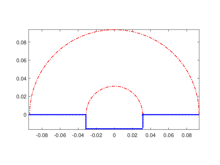
Refer to caption
Refer to caption
Figure 2. Example 1: (left) the cavity geometry; (right) the backscatter RCS for both cases by using the adaptive PML method and the adaptive TBC method.
Refer to caption
Refer to caption
Figure 3. Example 1: (left) the adaptive mesh after 3 iterations with a total number of nodal points 12591259; (right) the quasi-optimality of the a posteriori error estimates for both of the adaptive PML and TBC methods.
Refer to caption
Figure 4. Example 1: the ratio of DoFh{\rm DoF}_{h} between the physical domain and the whole computational domain.

5.2. Example 2

In this example, we also consider the TM polarization. The backscatter RCS for a coated rectangular cavity with width 2.4​λ2.4\lambda and depth 1.6​λ1.6\lambda is computed. The each vertical side of the cavity wall is coated with a thin layer of some absorbing material. Figure 5 illustrates the geometry of the cavity and PML setting. The coating on both sides has thickness 0.024​λ0.024\lambda and is made of a homogeneous absorbing material with a relative permittivity ϵr=12+0.144​i\epsilon_{\rm r}=12+0.144{\,\rm i} and a relative permeability μr=1.74+3.306​i\mu_{\rm r}=1.74+3.306{\,\rm i}. This example has a multi-scale feature and is an interesting benchmark example to test the adaptive method. We take the same stopping rule as that in Example 1: the adaptive method is stopped once the number of nodal points is over 15000. Figure 5 plots the backscatter RCS by using the adaptive PML and TBC methods, where the red solid line stands for the results of the PML method and the blue circles stand for the results of the TBC method. Clearly, these two methods are consistent with each other. Using a representative example of incident angle θ=π/4\theta=\pi/4, we present the refined mesh after 2 iterations with 1263 DoFh{\rm DoF}_{h} and the a posteriori error estimates in Figure 6. It is clear to note that the method can capture the behavior of the numerical solution in the two thin absorbing layers and displays the quasi-optimality between the meshes and the associated numerical complexity, i.e., ϵh=𝒪(DoFh−1/2)\epsilon_{h}=\mathcal{O}({\rm DoF}_{h}^{-1/2}) holds asymptotically. As a comparison, we also show the a posteriori error estimates of the adaptive TBC method in the red dashed line. The quasi-optimality is also observed for the adaptive TBC method. Figure 7 shows the ratio of DoFh{\rm DoF}_{h} between the physical domain and the whole computational domain. Again, we see that most nodal points are concentrated in the physical domain,r which illustrates the effectiveness of the adaptivity.
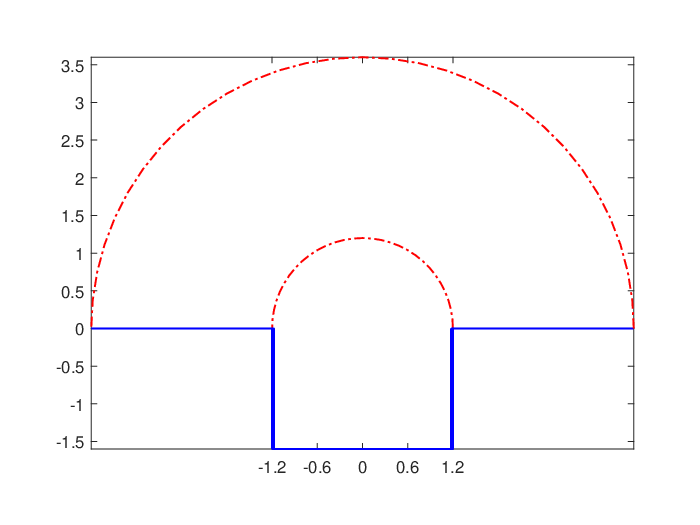
Refer to caption
Refer to caption
Figure 5. Example 2: (left) the cavity geometry; (right) the backscatter RCS by using the adaptive PML method and the adaptive TBC method.
Refer to caption
Refer to caption
Figure 6. Example 2: (left) the adaptive mesh after 2 iterations with a total number of nodal points 12631263; (right) the quasi-optimality of the a posteriori error estimates for both of the PML and TBC methods.
Refer to caption
Figure 7. Example 2: the ratio of DoFh{\rm DoF}_{h} between the physical domain and the whole computational domain.

5.3. Example 3

This example is still concerned with the TM polarization but some part of the structure for the cavity sticks out above the ground plane. The width and depth of the base cavity is 1.2​λ1.2\lambda and 0.8​λ0.8\lambda, respectively. There are two thin rectangular PEC humps in the middle of the cavity. Their width is 120​λ\frac{1}{20}\lambda and height is 1615​λ\frac{16}{15}\lambda and 815​λ\frac{8}{15}\lambda, respectively. The geometry of the cavity is shown in the left hand side of Figure 8. The backscatter RCS is computed by using the adaptive PML and the adaptive TBC method. We also use the red solid line for the PML method and blue circles for the TBC method. Using the incident angle θ=π/4\theta=\pi/4 as an example, we show the refined mesh after three iterations with the number of nodal points 1261 and the a posteriori error estimates in Figure 9. The adaptive PML method is able to refined meshes around the corners of the cavity where the solution has a singularity. The quasi-optimality is also obtained for the a posteriori error estimates. As a comparison, we show the a posteriori error estimates for the adaptive TBC method in the red dashed line. The observation of the a posteriori error estimates for both methods is the same as that in Examples 1 and 2. Finally, Figure 10 shows the ratio of DoFh{\rm DoF}_{h} between the physical domain and the whole computational domain. Once again, the example confirms the effectiveness of the adaptive method.
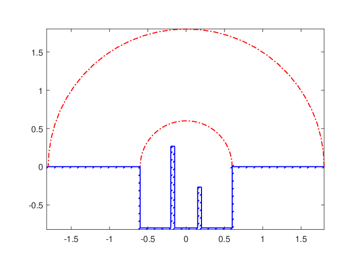
Refer to caption
Refer to caption
Figure 8. Example 3: (left) the cavity geometry; (right) the backscatter RCS by using the adaptive PML method and the adaptive TBC method.
Refer to caption
Refer to caption
Figure 9. Example 3: (left) the adaptive mesh after 3 iterations with a total number of nodal points 12611261; (right) the quasi-optimality of the a posteriori error estimates for both of the PML and TBC methods.
Refer to caption
Figure 10. Example 3: the ratio of DoFh{\rm DoF}_{h} between the physical domain and the whole computational domain.

5.4. Example 4

In this example, we consider the TE polarized cavity scattering problem. The cavity is a rectangle with a fixed width 0.025 m and a fixed depth 0.015 m. The cavity is empty with no filling materials. Instead of considering the illumination by a plane wave with a fixed frequency, we compute the backscatter RCS with the frequency ranging from 2 GHz to 18 GHz. Correspondingly, the range of the aperture of cavity is from 16​λ\frac{1}{6}\lambda to 1.5​λ1.5\lambda. The incident angle is fixed to be 49​π\frac{4}{9}\pi. Figure 11 shows the backward RCS by using the adaptive PML and the adaptive TBC method, where the red solid line and blue circles show their results, respectively. The stopping criterion is that the mesh refinement is stopped when the number of nodal points is over 25000. Once again, both methods are consistent with each other very well.

Refer to caption
Figure 11. Example 4: the backscatter RCS by using the adaptive PML method and the adaptive TBC method.

6. Conclusion

In this paper, we have presented an adaptive finite element PML method for solving the open cavity scattering problems. The a posteriori error analysis is carried out for both of the TM and TE polarizations. In each polarization, the estimate takes account of the finite element discretization error and the truncation error of PML method. The latter is shown to decay exponentially with respect to the PML medium parameter and the thickness of the layer. A possible future work is to extend our analysis to the adaptive finite element PML method for solving the three-dimensional cavity scattering problem, where the wave propagation is governed by Maxwell’s equations.

References

  • [1] M. Ainsworth and A. W. Craig, A posteriori error estimators in the finite element method, Numer. Math., 60 (1991), 429–463.
  • [2] M. Ainsworth and J. T. Oden, A unified approach to a posteriori error estimation using element residual methods, Numer. Math., 65 (1993), 23–50.
  • [3] I. Babuška and A. Aziz, Survey lectures on Mathematical Foundation of the Finite Element Method, in the Mathematical Foundations of the Finite Element Method with Application to the Partial Differential Equations, ed. by A. Aziz, Academic Press, New York, 1973, 5–359.
  • [4] I. Babuška and W. C. Rheinboldt, Error estimates for adaptive finite element, SIAM J. Numer. Anal., 15 (1978), 736–754.
  • [5] R. E. Bank and A. Weiser, Some a posteriori error estimators for elliptic partial differential equations, Math. Comp., 44 (1985), 283–301.
  • [6] G. Bao and H. Wu, Convergence analysis of the PML problems for time-harmonic Maxwell’s equations, SIAM. J. Numer. Anal., 43 (2005), 2121–2143.
  • [7] J.-P. Bérenger, A perfectly matched layer for the absorption of electromagnetic waves, J. Comput. Phys., 114 (1994), 185–200.
  • [8] J. Bramble and J. Pasciak, Analysis of a finite PML approximation for the three dimensional time-harmonic Maxwell’s and acoustic scattering problems, Math. Comp., 76 (2007), 597–614.
  • [9] J. Chen and Z. Chen, An adaptive perfectly matched layer technique for 3-D time-harmonic electromagnetic scattering problems, Math. Comp., 76 (2008), 673–698.
  • [10] Z. Chen and S. Dai, Adaptive Galerkin methods with error control for a dynamical Landau model in superconductivity, SIAM J. Numer. Anal., 38 (2001), 1961–1985.
  • [11] Z. Chen and S. Dai, On the efficiency of adaptive finite element methods for with discontinuous coefficients, SIAM J. Sci. Comput., 24 (2002), 443–462.
  • [12] Z. Chen and X. Liu, An adaptive perfectly matched layer technique for time-harmonic scattering problems, SIAM. J. Numer. Anal., 43 (2005), 645–671.
  • [13] Z. Chen and H. Wu, An adaptive finite element method with perfectly matched absorbing layer for the wave scattering by periodic structures, SIAM. J. Numer. Anal., 41 (2003), 799–826.
  • [14] Z. Chen and W. Zheng, PML Method for electromagnetic scattering problem in a two-layered medium, SIAM. J. Numer. Anal., 55 (2017), 2050–2084.
  • [15] F. Collino and P. Monk, Optimizing the perfectly matched layer, Comput. Methods Appl. Mech. Engrg., 164 (1998), 157–171.
  • [16] C. Collino and P. Monk, The perfectly matched layer in curvilinear coordinates, SIAM, J. Sci. Comput., 19(1998), 2061–2090.
  • [17] T. Hohage, F. Schmidt and L. Zschiedrich, Solving time-harmonic scattering problems based on the pole condition, II. Convergence of the PML methods, SIAM J. Appl. Math., 35 (2003), 547–560.
  • [18] J. Jin, The Finite Element Method in Electromagnetics, Wiley & Son, New York, 2002.
  • [19] M. Lassas and E. Somersalo, On the existence and convergence of the solution of the PML equations, Computing, 60 (1998), 229–241.
  • [20] P. Li, A survey of open cavity scattering problems, J. Comp. Math., 36 (2018), 1–16.
  • [21] P. Li, H. Wu, and W. Zheng, An overfilled cavity problem for Maxwell’s equations, Math. Meth. Appl. Sci., 15 (2012), 1951–1979.
  • [22] P. Monk, A posteriori error indicators for Maxwell’s equations, J. Comput. Appl. Math., 100 (1998), 173–190.
  • [23] P. Monk and E. Soli, The adaptive computation of far-field patterns estimation of linear functionals, SIAM J. Numer. Anal., 36 (1998), 251–274.
  • [24] F. Teixera and W. Chew, Systematic derivation of anisotropic PML absorbing media in cylindrical and spherical coordinates, IEEE Microw. Guided Wave Lett., 7 (1997), 371–373.
  • [25] E. Turkel and A. Yefet, Absorbing PML boundary layers for wave-like equations, Appl. Numer. Math., 27 (1998), 533–557.
  • [26] A. H. Schatz, An observation concerning Ritz-Galerkin methods with indefinite bilinear forms, Math. Comp., 28 (1974), 959–962.
  • [27] A. Wood, Analysis of electromagnetic scattering from an overfilled cavity in the ground plane, J. Comput. Phys., 215 (2006), 630–641.
  • [28] X. Yuan, G. Bao, and P. Li, An adaptive finite element DtN method for the open cavity scattering problems, CSIAM Trans. Appl. Math., to appear.