Formalizing the Soundness of the Encoding Methods of SAT-based Model Checking

Given a target system $(I,T)$, a property $P$ and a bound $k$, an SMC procedure encodes the safety of the system into a logic formula $F$ and checks its satisfiability using a SAT/SMT solver. This procedure can be summarized as Alg. 1. Each SMC method provides their own encoding method; therefore, in the algorithm, it is parameterized as $\mathsf{E}_{\bullet}$ at Line 1. An encoding method generates a formula $F$ that describes a given system and a property by considering only a finite number (which depends on $k$) of states. As a result, multiple validity problems of the form $\forall{s_{[0..m]}},{f_{i}}$ are generated as sub-formulas in $F$; then, they are discharged using a SAT/SMT solver, and those sub-formulas are substituted with the results, i.e. true or false (Line 3). Here, we denote the substitution of a sub-formula $G$ in $F$ with $H$ by $F\{G\mapsto H\}$; the validity problem is solved by checking the unsatisfiability of the negation of $f_{i}$. An encoded formula $F$ can be an arbitrary logical combination of the sub-formulas, e.g., $\neg(\forall{s_{[0..m]}},{f_{1}})\land(\forall{s_{[0..m]}},{f_{2}})\lor\cdots$. At Line 5, the validity of $F$ is determined, typically with a case analysis.

As a basic encoding method, we consider to encode a bounded safety property. For SMC with the bound $k$, we prepare $k\!+\!1$ state variables $s_{[0..k]}$. Then, the following predicate formula states that every sequence $s_{[0..i]}$, which represents an initial path fragment of length $k$ or less, reaches a safe state.

In the above, $I$, $T$ and $P$ are predicates on states that specify the target system model and the property. By running Alg. 1 with $\mathsf{E}_{\eqref{eq:ksafety}}$, which is supported by a SAT or SMT solver, we are able to verify whether the system is safe within the bound $k$ (R2) or there exists a counterexample (R3).

To use a SAT solver as the $\mathsf{CheckSat}$ procedure in Alg 1, the body of an encoded formula has to be (the negation of) a conjunction. Hence, the formula (3) should be modified as

which is equivalent to (3) in classical logic.

Encoding methods for unbounded safety that assume a set of lasso-shaped paths and apply an induction have been proposed. Sheeran et al.[2] have proposed six algorithms for this purpose, which are intended for an efficient encoding and reasoning of lasso-shaped paths. Some of the algorithms also utilize the $k$-induction principle for an efficient SMC.

First, we prepare a shorthand to describe that $s_{[o..k]}$ is a loop-free path.

Then, a sufficient condition for the safety (R1) can be encoded in two ways.

Either of the encoding methods $\mathsf{E}_{\eqref{eq:forward}}$ and $\mathsf{E}_{\eqref{eq:backward}}$ considers a fixed point of the reachability analysis from the initial states or the unsafe states, respectively. The second quantified sub-formula of $\mathsf{E}_{\eqref{eq:forward}}$ checks that all the initial paths of length $k$ contain a loop. The implication sub-formula of $\mathsf{E}_{\eqref{eq:backward}}$ is equivalent to $\neg P(s_{k})\to\neg\mathit{loopF}_{T}(s_{[0..k]})$ in classical logic; it checks that all paths of length $k$ from an unsafe state contain a loop. Since the safety within the bound $k$ is checked with $\mathsf{E}_{\eqref{eq:ksafety}}$, the safety R1 is inferred as a result. As for $\mathsf{E}_{\eqref{eq:ksafety}}$, we can modify the second parts of $\mathsf{E}_{\eqref{eq:forward}}$ and $\mathsf{E}_{\eqref{eq:backward}}$ as follows to have the sub-formulas of a conjunctive form.

Sheeran et al.’s first algorithm [2] is a hybrid method of the two, whose encoding method is equivalent to $\mathsf{E}_{\eqref{eq:forward}}\lor\mathsf{E}_{\eqref{eq:backward}}$. Sheeran et al.’s subsequent algorithms apply a $k$-induction and encode the safety as follows.

To have an unbounded model checker using our scheme of Alg. 2, $\mathsf{E}_{\bullet}$ in $\mathsf{Alg1}_{\mathrm{true}}$ can be implemented as either $\mathsf{E}_{\eqref{eq:forward}}$, $\mathsf{E}_{\eqref{eq:backward}}$, $\mathsf{E}_{\eqref{eq:kinduction}}$ or $\mathsf{E}_{\eqref{eq:forward}}\lor\mathsf{E}_{\eqref{eq:backward}}$, and it can be implemented as $\mathsf{E}_{\eqref{eq:ksafety}}$ in $\mathsf{Alg1}_{\mathrm{false}}$.

Bradley [4] has proposed an SMC method called IC3 or PDR (property directed reachability) [5] (we refer to the method as PDR in the sequel); it handles a sequence of over-approximations that encloses path fragments with sets of clauses; also, it uses the inductive relative relation between states to refine an over-approximation. In this paper, we do not go into the details of the method but focus on the post-conditions of the PDR method, given an over-approximation. We again adapt the method into our scheme of Alg. 1 and Alg. 2.

Assume a sequence $R_{0}R_{1}\cdots$ (denoted by $R_{[0..]}$ below) of over-approximations of a set of reachable states in $S$. Then, the post-condition of PDR for the true case is described as follows (we refer to the whole formula as (11) and to each sub-formula as (a)–(e)).

The original algorithm initializes over-approximations as $R_{0}\!:\leftrightarrow\!I$ and $R_{i}\!:\leftrightarrow\!P$ for $i\!\geq\!1$, and incrementally refines $R_{[0..(k+1)]}$ (for $k\!:=\!0,\ldots$). The algorithm repeatedly (i) detects a bad state $\tilde{s}$ such that $\exists\tilde{s}^{\prime},R_{k}(\tilde{s})\land T(\tilde{s},\tilde{s}^{\prime})\land\neg P(\tilde{s}^{\prime})$, (ii) generalizes $\neg\tilde{s}$ to a clause $C$ such that $\forall s,s^{\prime},R_{i}(s)\land C(s)\land T(s,s^{\prime})\to C(s^{\prime})$ (for some $i\leq k$), and (iii) refines $R_{[0..(i+1)]}$ by adding $C$ into the over-approximations. Finally, the algorithm terminates when the sub-formula (e) holds; the resulting over-approximation $R_{k}$ is an inductive strengthening of $P$, which is depicted in Fig. 1.

Note that the above post-condition is slightly modified from that of the original algorithm for the sake of simplicity of the verification process. First, although the original algorithm maintains a set of clauses for each $R_{i}$, we do not distinguish the set and $R_{i}$. Second, we weaken the sub-formula (e) from $\exists i\leq k,\forall s,~R_{i}(s)\leftrightarrow R_{i+1}(s)$.

The post-condition for the false case, which is extracted from the PDR algorithm, is described below (the sub-formulas are referred to as (a)–(c)).

The sub-formulas (a) and (b) are for detecting length 0 and 1 counterexamples. The sub-formula (c) describes initial and bounded safe paths of length $k$ or less, which is related with $R_{[0..(k-1)]}$.

Coq¹¹ 1 https://coq.inria.fr (version 8.6.1) is a proof assistant based on the typed lambda calculus, which supports predicate logic formulas, algebraic types, higher-order functions, etc. to describe theorems and proofs. Using the tactic mechanism, a proof can be described/performed efficiently and simply. In a part of the verification, we rely on the excluded middle axiom of the Classical_Prop module (see Sect. VI-C).

A plug-in software for Coq, coq2smt²² 2 https://github.com/wangjwchn/coq2smt (commit 604f72a), has developed to invoke SMT solvers within a Coq proof via the tactic smt solve. The tactic handles goals of a quantifier-free form involving boolean connectives, equalities, values/variables of type Z, etc.; it discharges a goal using an SMT solver (e.g. CVC4 and Z3) and reflects the result in the proof context of Coq.

To specify a state transition system $(I,T)$, its property $P$ and an over-approximation $R$, we assume the following types based on the definitions in Sect. II.

We specify the type state as Z to demonstrate a model checking using SMT solvers. To pursue the proof tasks in Sect. V, any type with equality = can be used as state. $I$, $P$ and $R$ are supposed to be typed as prop. For state sequences, we assume the following type.

Here, we have not drawn on existing abstract types (e.g. list) because, in our proof scheme for SMC (Sect. IV-C), we intend to expand a proof goal into a flat formula, instead of an inductive reduction. For instance, the predicate $\mathit{path}$ in Eq. (2), which requires a sequence $\texttt{ss}_{[\texttt{o}..(\texttt{len}-\texttt{o})]}$ to be a path fragment, is specified recursively as follows. Indeed, this enables an expansion with an unfold application given specific argument values.

Based on these types, for example, the method $\mathsf{E}_{\eqref{eq:forward}}$ is simply specified as the following predicate:

The predicates are defined separately for each sub-formula in Eq. (6); e.g., the predicate lasso_fwd is specified as

In this way, these predicates are able to be shared between different encoding methods. For example, a hybrid method of $\mathsf{E}_{\eqref{eq:forward}}$ and $\mathsf{E}_{\eqref{eq:backward}}$ is specified as follows.

A set of over-approximations (i.e. a sequence of prop values) handled by PDR is typed as the type spseq.

Using this type, for instance the body of the sub-formula $\mathsf{E}_{\eqref{eq:pdr:f}}$ (c) is specified as

In this section, we demonstrate that our specification works as a simple SMC tool (except for PDR as it requires to prepare an over-approximation). To do so, a user first specifies a verification problem by defining $I$, $T$ and $P$ as objects of the types trans and prop, respectively. Then, an SMC is performed by describing a theorem and its proof using a template script configured for each $\mathsf{E}_{\bullet}$. Type checking of this proof with Coq mimics an execution of the SMC procedure Alg. 1

For example, a template theorem and proof for SMC with forward_safety (Eq. (6)) is described as

Regarding Alg. 1, an $\mathsf{E}_{\bullet}$ method is implemented as a Coq predicate (e.g., forward_safety that implements $\mathsf{E}_{\eqref{eq:forward}}$), $\neg\mathsf{CheckSat}(\neg f)$ corresponds to discharging a sub-goal $f$ with smt solve, and $\mathsf{Decide}$ is represented as a proof template for each encoding method.

For the ease of proofs, we have developed vocabularies and lemmas on state sequences (of the type sseq) and paths (sseq values in which each pair of concatenated states satisfy $T$). Some of the lemmas utilized in the verification are shown in Fig. 2.

We introduce a suffix operation skipn for state sequences, which is defined as $\texttt{skipn}(i,s)_{[m..n]}:=s_{[(m+i)..(n+i)]}$, and formalize the related properties. Using skipn, we have the lemmas such as Fig. 2 (ss&p 1–3).

Various split operations for paths, loop-free paths, etc. are useful in the verification. Therefore, we formalize those split relations as lemmas; for instance, we have lemmas Fig. 2 (ss&p 4–6).

Let $k$ be the parameter of the encoding method. To prove Theorem 1 for either $\mathsf{E}_{\eqref{eq:forward}}$ or $\mathsf{E}_{\eqref{eq:backward}}$, we split either of the proof tasks into two cases $i\leq k$ and $i>k$, where $i$ is that in Lemma 1. We prove that the hypothesis in Lemma 1 holds for each case.

For the case $i\leq k$, we prove that the sub-formula $\mathsf{E}_{\eqref{eq:ksafety}}(I,T,P,k)$ implies the safety within the bound $k$. We perform an induction on $k$ to show the correspondence between $\mathsf{E}_{\eqref{eq:ksafety}}$, in which path is specified recursively, and the consequent specified with a universal quantifier.

For the case $i>k$, we split the path constraint in the proof context in either way of the following:

The split paths are illustrated in Fig. 3. The first $\mathit{loopF}_{T}$ of Eq. (13) (resp. the second $\mathit{loopF}_{T}$ of Eq. (14)) matches with the last sub-formula of Eq. (6) (resp. Eq. (7)). For Eq. 14, we utilize the skipn operator in the unification of formulas ($s_{[(i-k)..i]}$ is rewritten as $\texttt{skipn}(i,s)_{[0..k]}$). With the modifications of the proof contexts, the goals are discharged by matching them with the premises.

Theorem 1 with $\mathsf{E}_{\eqref{eq:kinduction}}$ is also proved with an application of Lemma 1 and a case split into $i\leq k$ and $i>k$.

The case $i\leq k$ is proved as in Sect. V-B.

For the case $i>k$, we apply a complete induction on the step number $i$ in the predicate $\mathit{safety}$; we are to prove that the $i$-th state satisfies the property $P$ assuming $\mathsf{E}_{\eqref{eq:kinduction}}$ and the safety within the depth $i\!-\!1$. The proof is done in three steps. First, we split the constraint $\mathit{loopF}_{T}(s_{[0..i]})$ in the proof context in two, $\mathit{loopF}_{T}(s_{[0..(i-k)]})$ and $\mathit{loopF}_{T}(s_{[(i-k)..i]})$, as in Eq. (13). Second, we modify the indices in the sub-formula of Eq. (10) with the lemma

Third, $P$ is inferred by applying the last sub-formula of Eq. (10) and the hypothesis of the complete induction.

Theorem 2 with $\mathsf{E}_{\eqref{eq:ksafety}}$ is proved by showing that $\mathsf{E}_{\eqref{eq:ksafety}}$ always hold when assuming the safety of a system. It is simply proved by an induction on $k\!+\!1$.

Theorem 1 with $\mathsf{E}_{\eqref{eq:pdr:t}}$ is proved by several case analyses and inductions as described below. At first, the proof goal is split into the two goals of the form

where $\circ$ is set as either $\leq$ or $>$. The consequence $R_{i}(s_{i})$ is obtained by applying $\mathsf{E}_{\eqref{eq:pdr:t}}$ (b) to the term $P(s_{i})$ in $\mathit{safety}$.

For the case $\circ:=\ \leq$, we perform an induction on $i$. The initial case is proved by $\mathsf{E}_{\eqref{eq:pdr:t}}$ (a). In the induction step where $i\!+\!1\leq k\!+\!1$, the proof context consists of the consequence $R_{i+1}(s_{i+1})$ and a set of hypotheses. $R_{i+1}(s_{i+1})$ is transformed to $R_{i}(s_{i})$ by $\mathsf{E}_{\eqref{eq:pdr:t}}$ (c). As a result, the proof context matches the induction hypothesis and be discharged.

For Eq. (15) with $\circ:=\ >$, we again perform an induction on $i$. The initial case ($0>k^{\prime}$, where $k:=k\!+\!1$) immediately holds. In the induction step ($i+1>k^{\prime}$), the goal $R_{k^{\prime}}(s_{i+1})$ is transformed into $R_{k^{\prime}}(\texttt{skipn}(i,s)_{1})$. Then, we have $R_{k}(\texttt{skipn}(i,s)_{0})=R_{k}(s_{i})$ by applying $\mathsf{E}_{\eqref{eq:pdr:t}}$ (d), and $R_{k^{\prime}}(s_{i})$ by rewriting with $\mathsf{E}_{\eqref{eq:pdr:t}}$ (e). Here, we consider two cases $i=k^{\prime}$ and $i>k^{\prime}$ separately. For the first case, the goal $R_{k^{\prime}}(s_{i})=R_{k^{\prime}}(s_{k^{\prime}})$ is proved by applying Eq. (15) with $i:=k^{\prime}$. For the case when $i>k^{\prime}$, we are able to deduce the goal $R_{k^{\prime}}(s_{i})$ from the induction hypothesis; so it is discharged.

Theorem 2 with $\mathsf{E}_{\eqref{eq:pdr:f}}$ is proved by showing that each of the three sub-formulas of $\mathsf{E}_{\eqref{eq:pdr:f}}$ holds when assuming the safety of a system.

The sub-formulas (a) and (b) are easy to prove.

Before the proof of the sub-formula $\mathsf{E}_{\eqref{eq:pdr:f}}$ (c), we prepare the following lemma that states a necessary condition.

Note that the hypothesis is the negation of the body of $\mathsf{E}_{\eqref{eq:pdr:f}}$ (c). It is proved by an induction on $k$; in the induction step, we prove by a case split into the cases $k=0$, $0=i<k$ and $0<k\leq i+1$.

The proof context of the sub-formula $\mathsf{E}_{\eqref{eq:pdr:f}}$ (c) contains the hypothesis part of Eq. (16), so it is rewritten into the consequence part of Eq. (16). The proof goal $P(s_{k+1})$ is discharged by the assumption of the safety, but we need to show additionally that $s_{[0..(k+1)]}$ is a path of the system. Using the rewritten premise above, we are able to prove it.

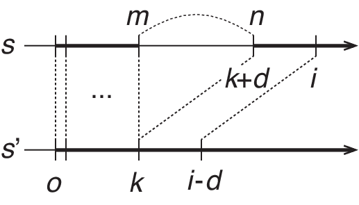
Lemma 1 is proved by a complete induction on $i$ in $\mathit{safety}$. In the induction step, we have to show the safety of the arbitrary paths of length $i\!+\!1$, assuming the safety within the lengths less than $i\!+\!1$ and the safety of the loop-free paths of length $i\!+\!1$. It is proved based on the observation that the reachable states by looped paths can be reached by a shorter path.

To compare paths with or without a loop reaching a same state, we introduce the predicate $\texttt{shorter\char 95\relax ss}(o,k,d,s,s^{\prime})$ defined as

Fig. 4 (left) illustrates the definition. It represents the fact that a sequence $s^{\prime}$ is a shortened sequence of $s$ where the fragment $s_{[(k+1)..(k+d-1)]}$ is removed from $s$; thus, two fragments of each of the two sequences coincide as $s_{[o..k]}=s^{\prime}_{[o..k]}$ and $s_{[(k+d)..]}=s^{\prime}_{[k..]}$.

With this predicate, we formalize the lemma

Note that the consequent part can be transformed into the formula below in classical logic.

Fig. 4 (right) illustrates this lemma. It states that, when a sequence $s$ contains a loop, there exists a shortened sequence $s^{\prime}$ and the same states are reachable with the two paths. The consequent holds by matching the variables as $k=m$ and $d=n-m$.

To prove Lemma 1, we perform a proof by contradiction; we assume that an unsafe path of length $k$ exists when the safety is checked for loop-free paths of length $k$. Such path should be looped; thus, we can show that there are unsafe shorter paths, which contradicts the induction hypothesis.

The LOC for each proof is shown in Table I; the third and sixth columns show the LOC of the proofs related to state sequences and paths described in Sect. V-A and V-G. For instance, the overall proof script for Theorem 1 with $\mathsf{E}_{\eqref{eq:forward}}$ consisted of 459 LOC, which involved the proof script for Lemma 1, three lemmas for the cases analyzed and 11 “ss&p” lemmas. Note that, many of the “ss&p” lemmas were shared between the different verification tasks.

The proof of Lemma 1 was formalized with 352 LOC, in which we reduced the lemma twice into other proof goals; the resulting goal was proved with nine “ss&p” lemmas.

We have successfully formalized the soundness proofs following the discussions in the original papers [2, 4]. In the formalization, we used the lemmas in Sect. V-A and V-G and they were reused in several proof tasks.

In the proofs, a number of inductions were performed based on the recursive definitions of the encoding predicates and the path lengths under consideration. In each induction step, proof context was carefully modified to apply prepared lemmas; in some proofs, rewriting with the skipn expression and applying path splitting lemmas were useful.

A fair amount of LOCs were devoted to Lemma 1 as it required to perform a proof by contradiction and translation between loop paths and shorter paths (Sect. V-G).

The proofs for PDR (Sect. V-E and V-F) consisted of a number of case analyses and inductions; the split goals were discharged by applying sub-formulas of $\mathsf{E}_{\eqref{eq:pdr:t}}$ and $\mathsf{E}_{\eqref{eq:pdr:f}}$. It was less often to describe paths explicitly in the proof contexts than the other methods and thus the resulting proofs became relatively small.

In the proof, we used several lemmas of the Classical_prop module. On the other hand, we tried to minimize the proofs that require those lemmas. As a result, we identified the two parts in the proofs: (i) the transformation into conjunctions at the front-end of each encoding method (e.g. from (3) to (4), from (6) to (8), etc.). (ii) the proof of Lemma 1. The other proofs were formalized without the use of classical logic.

We conjecture that the use of the law of excluded middle is essential in the parts (i) and (ii). In (ii), it was used to apply the law of double negation to perform a proof by contradiction, to obtain the contraposition of Eq. (17), and to decompose the negation of the loop_free clause.

References

- [1] A. Biere, A. Cimatti, E. M. Clarke, and Y. Zhu, “Symbolic Model Checking without BDDs,” in TACAS, LNCS 1579, 1999, pp. 193–207.
- [2] M. Sheeran, S. Singh, and G. Stålmarck, “Checking safety properties using induction and a SAT-solver,” in FMCAD, LNCS 1954, 2000, pp. 127–144.
- [3] K. L. McMillan, “Interpolation and SAT-Based Model Checking,” in CAV, LNCS 2725, 2003, pp. 1–13.
- [4] A. R. Bradley, “SAT-Based Model Checking Without Unrolling,” in VMCAI, 2011, pp. 70–87.
- [5] N. Een, A. Mishchenko, and R. Brayton, “Efficient implementation of property directed reachability,” in FMCAD, no. 1, 2011, pp. 125–134.
- [6] K. Claessen and N. Sorensson, “A liveness checking algorithm that counts,” in FMCAD, 2012, pp. 52–59.
- [7] A. Biere and D. Kröning, “SAT-Based Model Checking,” in Handbook of Model Checking. Springer, 2018, ch. 10, pp. 277–303.
- [8] M. Bozzano, R. Cavada, A. Cimatti, M. Dorigatti, A. Griggio, A. Mariotti, A. Micheli, S. Mover, M. Roveri, and S. Tonetta, “nuXmv 2.0.0 User Manual,” 2019.
- [9] A. Mebsout and C. Tinelli, “Proof Certificates for SMT-based Model Checkers for Infinite-state Systems,” in FMCAD, 2016, pp. 117–124.
- [10] K. S. Namjoshi, “Certifying Model Checkers,” in CAV, LNCS 2102, 2001, pp. 2–13.
- [11] C. Sprenger, “A Verified Model Checker for the Modal mu-calculus in Coq,” in TACAS, LNCS 1384, 1998, pp. 167–183.
- [12] H. Amjad, “Programming a Symbolic Model Checker in a Fully Expansive Theorem Prover,” in TPHOLs, LNCS 2758, 2003, pp. 171–187.
- [13] J. Esparza, P. Lammich, R. Neumann, T. Nipkow, A. Schimpf, and J.-G. Smaus, “A Fully Verified Executable LTL Model Checker,” in CAV, LNCS 8044, 2013, pp. 463–478.
- [14] S. Wimmer and P. Lammich, “Verified Model Checking of Timed Automata,” in TACAS, LNCS 10805, 2018, pp. 61–78.
- [15] M. Armand, G. Faure, B. Grégoire, C. Keller, and B. Werner, “A Modular Integration of SAT/SMT Solvers to Coq through Proof Witnesses,” in CPP, LNCS 7086, 2011, pp. 135–150.