Multi-Agent Reinforcement Learning for Cooperative Coded Caching via Homotopy Optimization

Prior studies generally investigated the potentials of edge caching by optimizing average performance criteria. For instance, the studies in [10, 11, 12] examined effective caching strategies to alleviate traffic loads, and to reduce system cost and download latency. With the aid of caching resources at SBSs, the studies in [13, 14] investigated the joint design of SBS beamforming and clustering. Caching strategies in these studies were designed to store either entire content items or uncoded fragments, which are referred to as uncoded caching.

To further improve caching efficiency, coded caching has recently gained considerable research attention. The study in [15] proposed a novel coded caching scheme, which provides a global caching gain relating to cumulative storage over all caching units. The research in [16, 17] investigated cooperative coded caching by utilizing maximum separable distance (MDS) codes to reduce traffic loads. MDS coded caching was also examined in [18, 19] to augment SBS collaboration and thus offers great advantages to lower latency and reduce power consumption compared with uncoded caching. The above-mentioned studies mainly investigated offline caching policies by assuming time-invariant content popularity distributions.

To exploit dynamic features in wireless networks, extant works have been devoted to designing caching policy by using RL. The study in [20] utilized Q-learning to find an optimal caching policy to minimize network cost. To counter the curse of dimensionality in conventional RL, DRL-based caching polices were advocated in [21, 9, 22, 23] by using deep neural networks (DNNs) as function approximators. Moreover, the study in [24] proposed a multi-agent DRL framework to maximize cache hit ratios for centralized and decentralized settings. The authors in [25] investigated cache placement by using cooperative multi-agent multi-armed bandit learning at small cell networks (SCN). A decentralized caching scheme was proposed in [26] by utilizing federated deep reinforcement learning. Nevertheless, the research in [20, 23, 21, 9, 22, 24, 25, 26] focused on uncoded caching. That is, each content item is entirely cached without exploring SBSs cooperatively fetching coded fragments of each content item.

Indeed, cooperatively pre-fetching MDS coded fragments has been proven to significantly alleviate traffic loads and thus reduce latency, as well as transmission cost over storing uncoded fragments at SCN [17, 19, 18]. Specifically, since one can distribute MDS coded fragments of a content item to multiple SBSs, mobile users can access a cluster of SBSs simultaneously to download coded fragments of the desired content item. To date, very few works have investigated how to “intelligently” update MDS coded content items under dynamic environments (e.g., time-varying content popularity). Under centralized control, a prior study [27] utilized deep deterministic policy gradient (DDPG) to explore MDS coded caching under dynamic content popularity with the aid of predicting user requests; and study [28] utilized Q-learning with function approximation to investigate coded caching.

It is worth noting that, unlike uncoded caching schemes [8, 7, 20, 21, 9, 22, 23, 24, 25] addressing binary decision-making, coded caching essentially entails continuous caching decisions that are subject to storage constraints. Accordingly, the resulting decision-making for dynamic coded caching is a constrained RL with a continuous action space. Quantizing actions into discrete values or directly applying conventional DRL algorithms may not be able to efficiently handle this constrained RL problem. In addition, a centralized control could lead to excessive communication overhead because the cloud processor (CP) needs frequent communications with SBSs to aggregate information and inform SBSs of their caching decisions. As the number of SBSs increases, the dimension of continuous states and actions in a centralized control would be very large, and optimal caching is computationally prohibitive. As a consequence, it is very challenging, but essential, to design efficient DRL algorithms for cooperative coded caching.

To bridge the research gap identified above, in this work, we investigate cooperative coded caching design at SCN with temporally evolving content popularity. In particular, we address the following fundamental issues for empowering “intelligent” caching: i) how to design efficient DRL algorithms for a constrained RL problem with continuous decision variables; and ii) how to develop a multi-agent DRL-based framework with different levels of controls to obtain an equitable trade-off between performance and complexity.

The main contributions of this work are summarized as follows:

1. $\bullet$

   To the best of our knowledge, this is the first work to investigate a multi-agent DRL framework for MDS coded caching under time-varying content popularity. Specifically, we model cache updating for MDS coded caching as a cooperative multi-agent Markov dynamic process (MDP). With the goal of minimizing long-term expected cumulative fronthaul traffic loads, we judiciously define the system state, local observations and action space of each agent, as well as caching reward. Our formulated problem is a continuous RL with action constraints. We also characterize optimal decisions in a closed form.

2. $\bullet$

   As a core technical contribution, we reformulate a general constrained RL problem, whose action space is inefficient to be satisfied through designing DNNs, into a tractable form that can be dealt with by utilizing homotopy optimization. Then, we custom-build a novel DRL, i.e., homotopy deep deterministic policy gradient (HDDPG), through recasting the basic elements of RL and unfolding the iterative process of homotopy optimization. The novelty of this approach lies in introducing a reasonable cumulative penalty to the objective of RL, and then properly manipulating it by using homotopy optimization.

3. $\bullet$

   To endow the proposed DRL caching framework with different levels of control, we generalize the proposed HDDPG from centralized control to partially and fully decentralized controls. Specifically, in the centralized control, the CP coordinates SBSs to conduct cache updating by using global information. To reduce complexity and communication overhead, we then propose a partially decentralized control by allowing SBSs to make decisions locally, but their polices are learned in a centralized manner. In the fully decentralized control, each SBS works as an independent learner and trains its caching policy independently based on local observations. The proposed decentralized controls could obtain a desirable trade-off between complexity and performance, and thus have the potential to handle large-scale wireless networks.

The remainder of this paper is organized as follows. Sec. II presents the problem statement. Sec. III introduces the proposed DRL. Sec. IV develops a centralized cooperative coded caching design. Sec. V proposes a partially decentralized caching design, and Sec. VI proposes a fully decentralized caching design. Sec. VII presents performance evaluations, and Sec. VIII concludes the paper.

As illustrated in Fig. 1, we consider a SCN, in which a total of $B$ SBSs are densely deployed and thus are capable of cooperatively providing communication services for users. Each SBS is endowed with a cache unit, which can cache popular content from the CP through a capacity-limited fronthaul. The CP is further connected to the core network through a backhaul. Suppose that a catalog of $F$ content items are available in CP. For ease of discussion, all of the content items are of the same size $s$ bits, and each cache unit has a storage of $L\times s$ bits. Let $\mathcal{B}=\{1,\cdots,B\}$ and $\mathcal{F}=\{1,\cdots,F\}$ denote the indices of SBSs and content items, respectively.

To reduce traffic loads on the capacity-limited fronthaul and provide better services for mobile users, SBSs can proactively cache popular content. By applying MDS codes, each content item of size $s$ bits is able to be encoded into a sufficiently long sequence of parity bits, and any $s$ parity bits are sufficient to reconstruct the original content item [18, 29, 17]. Moreover, in practice, MDS coding can be implemented by Raptor codes only with a very small redundancy [29, 30]. Therefore, SBSs with limited caching storage can cooperatively and collectively cache these coded parity bits, so as to satisfy user requests locally as much as possible. More precisely, we define the cache allocation matrix as $\boldsymbol{L}=[l_{f,b}]\in\mathbb{R}^{F\times B}$, where element $l_{f,b}\in[0,1]$ denotes the proportion of parity bits encoding content item $f$ that are stored at SBS $b$, $\forall b\in\mathcal{B},f\in\mathcal{F}$. Owing to the storage limit at SBSs, cache allocation needs to satisfy $\sum_{f\in\mathcal{F}}l_{f,b}\leq L,\forall b$. It is worth noting that, the parity bits of a content item available at SBS $b$ should be independent of that cached at other SBSs; thus, users can always download distinct coded content items from multiple SBSs [17]. To guarantee this caching diversity among SBSs, the encoded information sequence of parity bits of every content item should be sufficiently long, e.g., larger than $Bs$.

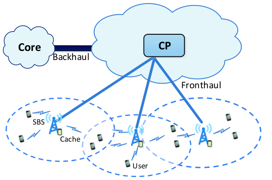
In what follows, we introduce how SBSs cooperatively transmit coded content items to mobile users. Specifically, the operation cycle of a SCN is slotted into a series of epochs, indexed by $t=0,1,\cdots$. For each epoch $t$, a number of active users $\mathcal{K}^{t}$ are randomly distributed in the horizontal plane. We also assume that the duration of each epoch is relatively short, such that active users are considered to be quasi-static during a single epoch. Each user $k\in\mathcal{K}^{t}$ is able to be served by a local SBS cluster, which is specified by the communication radius [31]. Therefore, network connectivity for epoch $t$ is denoted by $\mathcal{E}^{t}=\{e_{k,b}^{t}\}_{k\in\mathcal{K}^{t},b\in\mathcal{B}}$; each element $e_{f,b}^{t}=1$ if $d_{k,b}^{t}\leq r_{0}$, where $r_{0}$ denotes the communication radius of each SBS, and $d_{k,b}^{t}$ denotes the distance between user $k$ and SBS $b$; otherwise, $e_{f,b}^{t}=0$. For notational convenience, we collect all active users served by SBS $b$ at epoch $t$ as set $\mathcal{K}_{b}^{t}=\{k\in\mathcal{K}^{t}|e_{k,b}^{t}=1\}$, for $\forall b\in\mathcal{B}$. Each user $k\in\mathcal{K}^{t}$ is assumed to request one content item at a single epoch. Evidently, when content item $f$ is not fully stored at user $k$ neighboring SBSs, i.e.,

the missing part ($1-\sum_{b\in\mathcal{B}}l_{f,b}e_{f,b}^{t})s$ needs to be transmitted by the CP via fronthaul. This event is referred to as cache miss, which introduces additional fronthaul traffic loads. We summarize all of the key notations¹¹ 1 Without further definition, in this paper, notation $(\cdot)^{t}$ denotes the value of $(\cdot)$ taken at epoch $t$. in Table I.

As a result, to mitigate traffic burden on fronthaul, optimized caching policies depend highly on knowledge of network connectivity, i.e., $\mathcal{E}^{t}$, and content popularity, i.e., $\{p_{f},\forall f\}$, where $p_{f}$ denotes the probability of content item $f$ being requested. These elements generally exhibit unknown and time-varying dynamics in practice. Indeed, caching content needs to be temporally updated based on historical observations in order to provide better download services for future requests. We thereby introduce a dynamic cooperative coded caching problem in the following subsection.

In the cooperative coded caching, SBSs are anticipated to collaboratively cache the coded content items, which can be specified by optimizing continuous variables $\{l_{f,b}^{t}\}$. Therefore, we formulate the considered cooperative coded caching problem as a cooperative multi-agent MDP.

As aforementioned, user requests are expected to be satisfied by SBSs locally as much as possible; otherwise, the missing fragments could introduce additional traffic burden and transmission delay on the fronthaul. Therefore, in this paper, our goal is to minimize the expected fronthaul traffic loads. Accordingly, the basic elements in a cooperative multi-agent MDP are defined as follows.

DDPG is one of the policy-based RL algorithms, which is widely used to handle continuous decision-making [32]. Built upon actor-critic architectures, this algorithm employs DNNs as function approximators to learn a deterministic policy that can map high-dimensional states into feasible continuous actions. Typically, a DDPG-based RL framework consists of two networks, i.e., critic and actor, which are detailed as follows.

For a class of RL problems, the corresponding action space $\mathcal{A}$ could be some constraints inefficient to be directly satisfied through designing DNNs, i.e., $\mu_{\boldsymbol{\theta}}$. More specifically, we consider the following situation: let set $\mathcal{A}_{\boldsymbol{\theta}}$ collect all of the proto-actions as a result of $\mu_{\boldsymbol{\theta}}(\boldsymbol{S}),\forall\boldsymbol{S}\in\mathcal{S}$; and feasible actions $\boldsymbol{A}$ may only lie on a subset of $\mathcal{A}_{\boldsymbol{\theta}}$, i.e., $\mathcal{A}\subseteq\mathcal{A}_{\boldsymbol{\theta}}$. To deal with this issue, a straightforward approach is to use a mapping function $\sigma_{\mathcal{A}}(\cdot)$, which can project a proto-action $\mu_{\boldsymbol{\theta}}(\boldsymbol{S})$ into the action space, i.e., $\sigma_{\mathcal{A}}\left[\mu_{\boldsymbol{\theta}}(\boldsymbol{S})\right]\in\mathcal{A}$. Thus, a feasible policy function can be given by $\pi_{\boldsymbol{\theta}}(\cdot)=\sigma_{\mathcal{A}}[\mu_{\boldsymbol{\theta}}(\cdot)]$. Accordingly, the associated policy-based RL problem is supposed to take the following form:

Nevertheless, for many constrained RL applications, poor actions are likely to be generated after projection. Like the example in the previous subsection, mapping a proto-action with a dominant element $a_{f,b}^{t}=L$ into an one-hot vector may lead to a very sparse caching vector; this case implies a very low caching resource available at SBSs. When frequently encountering this instance during training, using mapping methods may not guarantee network parameters to be efficiently updated. Thus, it will lead to a suboptimal policy.

To remedy this method, a natural idea is to seek a proper way to penalize the performance loss caused by mapping a proto-action $\mu(\boldsymbol{S}^{t})$ into a feasible one given any state $\boldsymbol{S}^{t}$. Let $g(\cdot|\sigma_{\mathcal{A}})$ be a general penalty function, which needs to be designed according to the corresponding problem. In the coded caching problem, inspired by Proposition 1, a penalty function can be given by

where $\|\cdot\|_{1}$ denotes $l_{1}$-norm; and this penalty indicates the remaining storage over all caching units after taking action $\sigma_{\mathcal{A}}(\boldsymbol{A})$.

The proposed approach is then built upon maximizing a homotopy function:

where the discount cumulative penalty, i.e., $G=\mathbb{E}\left[\sum_{t=0}^{+\infty}(\gamma)^{t}g(\boldsymbol{S}^{t}|\sigma_{\mathcal{A}})\right]$, is finite due to a discount factor $\gamma\in[0,1)$; and $\lambda\leq 0$ is a homotopy variable, such that:

At this stage, we introduce the following lemma to address problem (12) through a typical homotopy optimization method [33].

The motivation of the homotopy optimization approach is follows: Starting with a sufficient small value of $\lambda_{\min}<0$, a very large cumulative penalty $|\lambda_{\min}G|$ may penalize the corresponding policy (parametrized by ${\boldsymbol{\theta}^{0}}$) to generate intended actions, e.g., caching decisions that fully exploit available caching storage in the considered problem. Thereafter, by using homotopy optimization, we attempt to carefully tune policy parameter ${\boldsymbol{\theta}^{0}}$ to a (local) optimizer $\boldsymbol{\theta}^{I}$ of the original problem (12), which is likely to produce good decisions despite of applying mapping function $\sigma_{\mathcal{A}}(\cdot)$.

In each iteration of homotopy optimization, computing an optimizer (e.g.,$\boldsymbol{\theta}^{i}$) of problem (14) offline is somehow impractical under an unknown temporally evolving environment. For this reason, we custom-build HDDPG for problem (12) by recasting the basic elements of DRL and unfolding the iterative procedure of homotopy optimization introduced in Lemma 1.

Specifically, as an actor-critic approach, HDDPG maintains a parametrized critic $Q_{\text{hom},\boldsymbol{\phi}}(\boldsymbol{S},\boldsymbol{A})$ and actor $\mu_{\boldsymbol{\theta}}(\boldsymbol{S})$ in addition to a mapping function $\sigma_{\mathcal{A}}(\cdot)$, where a feasible policy is given by $\pi_{\boldsymbol{\theta}}(\boldsymbol{S})=\sigma_{\mathcal{A}}[\mu_{\boldsymbol{\theta}}(\boldsymbol{S})]$. Following the sketch of a plain DDPG,²² 2 For clarity, we term the DRL algorithm proposed in [32] as plain DDPG. we introduce the proposed algorithm as follows. Evidently, the objective $J_{\text{hom}}(\boldsymbol{\theta}|\lambda,\sigma_{\mathcal{A}})$ can be equivalently reformulated as:

Accordingly, we define the homotopy reward after taking action $\boldsymbol{A}^{t}$ as:

which is known at epoch $t+1$. Then, the homotopy Q-function can be given by:

which implies the discount cumulative homotopy reward after taking an action $\boldsymbol{A}^{t}$ under state $\boldsymbol{S}^{t}$ and thereafter following policy $\pi_{\boldsymbol{\theta}}(\cdot)=\sigma_{\mathcal{A}}[\mu_{\boldsymbol{\theta}}(\cdot)]$. As a direct deduction of the Bellman optimality equation [34], we have the following Homotopy Bellman Optimality Equation.

Accordingly, to estimate an optimal homotopy Q-function, the critic $Q_{\text{hom},\phi}(\boldsymbol{S},\boldsymbol{A})$ can be learned by using Lemma 2. Specifically, we update $\boldsymbol{\phi}$ by minimizing the following loss function:

where $\xi_{\text{hom}}=(\boldsymbol{S},\boldsymbol{A},R_{\text{hom}},\boldsymbol{S}^{\prime})$; and $y$ denotes the target value:

Regarding the update of the actor, it depends on the gradient of the objective $J_{\text{hom}}(\boldsymbol{\theta}|\lambda,\sigma_{\mathcal{A}})$, which brings us to the following the Deterministic Policy Gradient Theorem for HDDPG.

Finally, we leverage inexact gradient descent methods to update $\{\boldsymbol{\theta},\boldsymbol{\phi},\lambda\}$ [35]. In particular, the updates of $\boldsymbol{\phi},\boldsymbol{\theta}$ occur at each epoch, i.e.:

where $\alpha_{c}$ and $\alpha_{a}$ are the learning rates of the critic and actor, respectively; and $\lambda$ can be updated by a slow circle, i.e., after every $I_{0}$ epochs, one can execute the following:

where sequence $\{\lambda^{i}\}_{i=1}^{I}$ should meet the equality in (16).

In the ensuing sections, we will apply HDDPG to the cooperative coded caching problem and propose a centralized caching design, and further generalize HDDPG in decentralized settings to reduce complexity and communication cost.

The system operation includes two procedures, i.e., network training and network evaluation. In general, during network evaluation, the CP simply leverages the actor and mapping function to make caching decisions, while the critic is only necessary during training procedure to fine-tune the actor. The details of network design and training procedure are introduced as follows.

In the proposed centralized caching design, the CP needs to frequently communicate with SBSs during network training and evaluation. Herein, we briefly analyze fronthaul communication complexity of this centralized control, which is described by the total dimension of variables that are transmitted between the CP and SBSs. We consider the worst case, in which each SBS is fully loaded and serves a maximum number of users, e.g., $|\mathcal{K}_{b}^{t}|=K$. Specifically, during network training, the CP needs to obtain information about the system state $[\{f_{k}^{t}\},\mathcal{E}^{t},\boldsymbol{L}^{t}]$ at each epoch. The dimension of user requests should be $BK$. Network connectivity $\mathcal{E}^{t}$ can be computed by knowing the coordinates of the active users; by denoting the coordinates as two dimensional vectors, the total dimension of user positions is $2BK$. Clearly, the CP has the exact information about cache allocation $\boldsymbol{L}^{t}$, which is termed as $\boldsymbol{A}^{t-1}$ in its RB; thus, no fronthaul cost is involved. Afterwards, the CP uses the the fronthaul to inform caching decisions $\{\boldsymbol{A}_{b}^{t}\}$; the total dimension of the involved variables is given by $BF$. Regarding reward $R^{t+1}$, it can be inferred from state $\boldsymbol{S}^{t+1}$. Hence, the overall fronthaul communication complexity during network training is $\mathcal{O}(3BK+BF)$. When the system runs in an evaluation procedure, the CP again needs to know the system state and inform each SBS of its caching decision. Consequently, the corresponding fronthaul communication complexity is $\mathcal{O}(3BK+BF)$.

Moreover, the critic and actor are built upon system states and joint actions, i.e., $(\boldsymbol{S}^{t},\boldsymbol{A}^{t})$, which is in the order of $\mathcal{O}(B^{2})$ of local observations and actions, i.e., $(\boldsymbol{S}^{t}_{b},\boldsymbol{A}_{b}^{t})$. For this reason, the computational complexity would be excessively high as the number of agents increases for a continuous RL problem [37]. To address this issue, we now focus on developing efficient decentralized algorithms in following sections.

In a PD multi-agent framework, each agent maintains an actor and mapping function to produce its actions. To augment collaboration among multiple agents, these actors are trained with the aid of a (centralized) critic. Specifically, agent $b$ has an actor $\mu_{b}$ (parametrized by $\boldsymbol{\theta}_{b}$) and mapping function⁴⁴ 4 For simplicity of notation, $\mu_{b}$ and $\sigma_{b}$ are abbreviations of $\mu_{\boldsymbol{\theta}_{b}}$ and $\sigma_{\mathcal{A}_{b}}$, respectively. $\sigma_{b}$, which are able to map a (local) proto-action $\mu_{b}(\boldsymbol{S}_{b})$ into the corresponding action space $\mathcal{A}_{b}$. Accordingly, the policy function for agent $b$ can be expressed by $\pi_{b}=\sigma_{b}[\mu_{b}(\cdot)]$.

On the basis of homotopy optimization, all agents cooperatively seek polices to jointly maximize the following homotopy function:

where we define $\mu_{\boldsymbol{\theta}}\triangleq\{\mu_{1},\cdots,\mu_{B}\}$ and $\sigma_{\mathcal{A}}\triangleq\{\sigma_{1},\cdots,\sigma_{B}\}$; and the homotopy reward $R_{\text{hom}}^{t}$ can be given by (19). Next, a (centralized) critic $Q_{\text{hom},\boldsymbol{\phi}}(\boldsymbol{S}^{t},\boldsymbol{A}_{1}^{t},\boldsymbol{A}_{2}^{t},\cdots,\boldsymbol{A}_{b}^{t})$ is leveraged to estimate $\mathbb{E}\left[\sum_{\tau=0}^{\infty}(\gamma)^{t+\tau}R_{\text{hom}}^{t+\tau+1}\big|\boldsymbol{S}^{t},\boldsymbol{A}_{b}^{t},\mu_{b},\sigma_{b},\forall b\in\mathcal{B}\right].$ Similar to C-HDDPG, parameter $\boldsymbol{\phi}$ can be learned by minimizing the following loss function:

where $y_{\boldsymbol{\phi}^{-}}^{t}$ denotes the target value, i.e., $R_{\text{hom}}^{t+1}+\lambda Q_{\text{hom},\boldsymbol{\phi}^{-}}\left(\boldsymbol{S}^{t+1},\boldsymbol{A}_{1},\cdots,\boldsymbol{A}_{b}\right)\big|_{\boldsymbol{A}_{b}=\sigma_{b}[\mu_{b}^{-}(\boldsymbol{S}_{b}^{t+1})]},$ and $\boldsymbol{\theta}_{b}^{-},\boldsymbol{\phi}^{-}$ are parameters of target actor $\mu_{b}^{-}$ and target critic $Q_{\text{hom},\boldsymbol{\phi}^{-}}$, respectively. Furthermore, the gradient for training parameter $\boldsymbol{\theta}_{b}$ can be approximated by:

Similarly, homotopy variable $\lambda$ should be updated in accordance with (27).

As depicted in Fig. 2 (b), we propose a PD-HDDPG-based cooperative coded caching design. Specifically, the CP maintains a centralized (critic), while each SBS has a local actor and mapping function. In addition, the actor and mapping function are designed in the same manner as the centralized scheme to ensure that their outputs are feasible to (4). Particularly, $\sigma_{b}(\cdot)=\min\{\boldsymbol{1}_{F},\cdot\},\forall b\in\mathcal{B}$. During the training procedure, the critic and (local) actors should be learned in the CP. We again adopt the techniques of exploration and RB, and the entire procedure is similar to what we have presented in Algorithm 1. The detailed implementation is shown in Algorithm 2. Notably, after all actors are fine-tuned, the CP needs to send actor parameters (e.g., $\boldsymbol{\theta}_{b},\forall b$) to SBSs, which thereafter can locally compute actions.

During the training procedure, fronthaul communication complexity is the same as that of C-HDDPG, i.e., $\mathcal{O}(3BK+BF)$. When the system runs in an evaluation procedure, each SBS computes its action locally; obviously, no fronthaul communication is incurred when observing content requests and positions of local users.

As shown in Fig 2(c), each SBS has a set of critic, actor, and mapping functions. These basic elements are designed in the same manner as that of C-HDDPG, but built upon local observations. More precisely, with an actor $\mu_{b}(\cdot)$ and mapping function $\sigma_{b}$, SBS $b$ can obtain a feasible action by mapping a proto-action $\mu_{b}(\boldsymbol{S}_{b})$ into the action space $\mathcal{A}_{b}$, i.e., $\sigma_{b}[\mu_{b}(\boldsymbol{S}_{b})]$. SBSs are encouraged to cooperate with each other and receive a common reward $R^{t}$ from the environment as the performance criterion to evaluate their policies. On the basis of homotopy optimization, a (local) critic $Q_{\text{hom},\boldsymbol{\phi}_{b}}(\boldsymbol{S}_{b}^{t},\boldsymbol{A}_{b}^{t})$ is designed for SBS $b$ to estimate $\mathbb{E}\left[\sum_{\tau=0}^{+\infty}(\gamma)^{t+\tau}R_{\text{hom}}^{t+\tau+1}|\boldsymbol{S}_{b}^{t},\boldsymbol{A}_{b}^{t},\mu_{b},\sigma_{b}\right],$ where $R_{\text{hom}}^{t}$ is defined as:

and $g_{b}(\mathbf{S}_{b}^{t-1}|\sigma_{b})\triangleq L-\|\sigma_{b}(\mu_{b}(\boldsymbol{S}_{b}^{t-1}))\|_{1},\forall b$. Subsequently, each agent is envisioned to independently train its critic and actor. In addition, the training procedure should follow the same workflow as C-HDDPG, which is presented in Algorithm 3 in greater detail.

During network training, although fronthaul communications are not necessary for SBSs to obtain local observations, each SBS still needs to know the homotopy reward. SBSs first locally computes $\{g_{b}(\boldsymbol{S}_{b}^{t}|\sigma_{b})\}$, which are then aggregated by the CP and subsequently sent back to each SBS. Therefore, fronthaul communication complexity during training is given by $\mathcal{O}\left(2B\right)$. For network evaluation, SBSs can directly calculate local actions according to their observations; thus, no fronthaul communication is needed.

Unless stated otherwise, we consider the following default settings: a SCN covers a square area of $[0,1]$ km $\times$ $[0,1]$ km; four SBSs are uniformly deployed in the region, each of which has a communication radius of $r_{0}=500$ m and can provide service for a maximum of 100 mobile users during each epoch; and mobile users are randomly distributed by following PPP with density $9.5\times 10^{-5}$ during each epoch. Moreover, user preferences towards content are considered to have multiple patterns, i.e., each preference pattern follows a Zipf distribution, i.e., $p_{f}=\zeta_{f}^{-\kappa}/\sum_{f^{\prime}\in\mathcal{F}}\zeta_{f^{\prime}}^{-\kappa}$, where $\zeta_{f}$ denotes the popularity rank of content item $f$, which is temporally and randomly evolving as time passes; $\kappa$ denotes a skewness factor and randomly takes a value from $\{0.5,1,1.5,2\}$; a catalog of 20 content items are encoded by MDS codes; and each SBS has a fractional caching capacity $L/F=0.2$, which indicates that each SBS can fetch $20\%$ of the total content.

To analyze the proposed caching framework, we consider the following baselines:

• •

  Centralized Optimization-Cache Updating (CO-CU): This is a centralized optimization-based design, which is performed in the CP [17, 18]. Specifically, one can first estimate the probability of each content item that could be requested by users under the coverage of SBS $b$, i.e., $p_{f,b}=N_{f,b}/\sum_{f^{\prime}\in\mathcal{F}}N_{f^{\prime},b},\forall f$, where $N_{f,b}$ denotes how many requests of content item $f$ that SBS $b$ receives at the current epoch. Then, similar to the cooperative caching problem formulated in [17], the joint caching decision (e.g. $\boldsymbol{A}^{t}$) can be optimized by minimizing the expected fronthaul traffic loads together with cache updating cost.

• •

  Local Optimization-Cache Updating (LO-CU): This scheme works at a level of decentralized control. Instead of optimizing joint action $\boldsymbol{A}^{t}$ via CP in CO-CU, each SBS separately calculates its caching decision (e.g, $\boldsymbol{A}_{b}^{t}$) by minimizing the expected fronthaul loads corresponding to local user requests from its communication range.

• •

  Random Cache Updating (RCU): At each epoch, every SBS randomly updates its caching resource until it reaches storage limits.

• •

  Plain DDPG-Based Schemes: To assess the effectiveness of the proposed DRL, we consider to implement plain DDPG in different levels of controls, i.e., C-DDPG, PD-DDPG and FD-DDPG, each of which follows a similar idea to the proposed caching approach.

References

- [1] C. V. N. Index, “Cisco visual networking index: Global mobile data traffic forecast update, 2016–2021,” link: http://goo.gl/ylTuVx, 2017.
- [2] E. Bastug, M. Bennis, and M. Debbah, “Living on the edge: The role of proactive caching in 5G wireless networks,” IEEE Commun. Mag., vol. 52, no. 8, pp. 82–89, Aug. 2014.
- [3] D. Liu, B. Chen, C. Yang, and A. F. Molisch, “Caching at the wireless edge: design aspects, challenges, and future directions,” IEEE Commun. Mag., vol. 54, no. 9, pp. 22–28, Sept. 016.
- [4] J. Li, Y. Chen, Z. Lin, W. Chen, B. Vucetic, and L. Hanzo, “Distributed caching for data dissemination in the downlink of heterogeneous networks,” IEEE Trans. Commun., vol. 63, no. 10, pp. 3553–3568, Oct. 2015.
- [5] J. Li, H. Chen, Y. Chen, Z. Lin, B. Vucetic, and L. Hanzo, “Pricing and resource allocation via game theory for a small-cell video caching system,” IEEE J. Sel. Areas Commun., vol. 34, no. 8, pp. 2115–2129, Oct., 2016.
- [6] C. Bettstetter, “Mobility modeling in wireless networks: categorization, smooth movement, and border effects,” ACM SIGMOBILE Mob. Comput. Commun. Rev., vol. 5, no. 3, pp. 55–66, Jan. 2001.
- [7] V. Mnih, K. Kavukcuoglu, D. Silver, A. A. Rusu, J. Veness, M. G. Bellemare, A. Graves, M. Riedmiller, A. K. Fidjeland, G. Ostrovski et al., “Human-level control through deep reinforcement learning,” Nature, vol. 518, no. 7540, p. 529, Feb. 2015.
- [8] N. C. Luong, D. T. Hoang, S. Gong, D. Niyato, P. Wang, Y.-C. Liang, and D. I. Kim, “Applications of deep reinforcement learning in communications and networking: A survey,” IEEE Commun. Surveys Tuts., vol. 21, no. 4, pp. 3133–3174, Fourthquarter 2019.
- [9] A. Sadeghi, G. Wang, and G. B. Giannakis, “Deep reinforcement learning for adaptive caching in hierarchical content delivery networks,” IEEE Trans. Cogn. Commun. Netw., vol. 5, no. 4, pp. 1024–1033, Dec. 2019.
- [10] B. Blaszczyszyn and A. Giovanidis, “Optimal geographic caching in cellular networks,” in Proc. IEEE Int. Conf. Commun., June 2015, pp. 3358–3363.
- [11] X. Li, X. Wang, S. Xiao, and V. C. Leung, “Delay performance analysis of cooperative cell caching in future mobile networks,” in Proc. IEEE Int. Conf. Commun., Jane 2015, pp. 1–6.
- [12] X. Li, X. Wang, and V. C. Leung, “Weighted network traffic offloading in cache-enabled heterogeneous networks,” in Proc. IEEE Int. Conf. Commun., May 2016, pp. 1–6.
- [13] M. Tao, E. Chen, H. Zhou, and W. Yu, “Content-centric sparse multicast beamforming for cache-enabled cloud RAN,” IEEE Trans. Wireless Commun., vol. 15, no. 9, pp. 6118–6131, Sept. 2016.
- [14] X. Wu, X. Li, Q. Li, V. C. Leung, and P. Ching, “Latency driven fronthaul bandwidth allocation and cooperative beamforming for cache-enabled cloud-based small cell networks,” in Proc. IEEE Int. Conf. Acoust., Speech, and Signal Process., May, 2019, pp. 4594–4598.
- [15] M. A. Maddah-Ali and U. Niesen, “Fundamental limits of caching,” IEEE Trans. Inf. Theory, vol. 60, no. 5, pp. 2856–2867, May 2014.
- [16] V. Bioglio, F. Gabry, and I. Land, “Optimizing MDS codes for caching at the edge,” in Proc. IEEE Global Commun. Conf., Dec. 2015, pp. 1–6.
- [17] J. Liao, K.-K. Wong, Y. Zhang, Z. Zheng, and K. Yang, “Coding, multicast, and cooperation for cache-enabled heterogeneous small cell networks,” IEEE Trans. Wireless Commun., vol. 16, no. 10, pp. 6838–6853, Oct. 2017.
- [18] X. Wu, Q. Li, X. Li, V. C. Leung, and P. Ching, “Joint long-term cache updating and short-term content delivery in cloud-based small cell networks,” IEEE Trans. Commun., vol. 68, no. 5, pp. 3173 – 3186, May 2020.
- [19] X. Wu, Q. Li, V. C. Leung, and P. Ching, “Joint fronthaul multicast and cooperative beamforming for cache-enabled cloud-based small cell networks: An MDS codes-aided approach,” IEEE Trans. Wireless Commun., vol. 18, no. 10, pp. 4970–4982, Oct. 2019.
- [20] A. Sadeghi, F. Sheikholeslami, and G. B. Giannakis, “Optimal and scalable caching for 5G using reinforcement learning of space-time popularities,” IEEE J. Sel. Topics Signal Process., vol. 12, no. 1, pp. 180–190, Feb. 2018.
- [21] Y. He, Z. Zhang, F. R. Yu, N. Zhao, H. Yin, V. C. Leung, and Y. Zhang, “Deep-reinforcement-learning-based optimization for cache-enabled opportunistic interference alignment wireless networks,” IEEE Trans. Veh. Technol., vol. 66, no. 11, pp. 10 433–10 445, Nov. 2017.
- [22] Y. Wei, F. R. Yu, M. Song, and Z. Han, “Joint optimization of caching, computing, and radio resources for fog-enabled iot using natural actor-critic deep reinforcement learning,” IEEE Internet Things J., Apr. 2018.
- [23] P. Wu, J. Li, L. Shi, M. Ding, K. Cai, and F. Yang, “Dynamic content update for wireless edge caching via deep reinforcement learning,” IEEE Commun. Lett., vol. 23, no. 10, pp. 1773–1777, Oct. 2019.
- [24] C. Zhong, M. C. Gursoy, and S. Velipasalar, “Deep reinforcement learning based edge caching in wireless networks,” IEEE Trans. Cogn. Commun. Netw., Mar. 2020.
- [25] X. Xu, M. Tao, and C. Shen, “Collaborative multi-agent multi-armed bandit learning for small-cell caching,” arXiv preprint arXiv:2001.03835, 2020.
- [26] X. Wang, C. Wang, X. Li, V. C. Leung, and T. Taleb, “Federated deep reinforcement learning for internet of things with decentralized cooperative edge caching,” IEEE Internet Things J., Apr., 2020.
- [27] Z. Zhang and M. Tao, “Accelerated deep reinforcement learning for wireless coded caching,” in Proc. IEEE/CIC Int. Conf. Commun. in China, Sept. 2019, pp. 249–254.
- [28] S. Gao, P. Dong, Z. Pan, and G. Y. Li, “Reinforcement learning based cooperative coded caching under dynamic popularities in ultra-dense networks,” IEEE Trans. Veh. Technol., vol. 69, no. 5, pp. 5442–5456, May 2020.
- [29] A. Liu and V. K. Lau, “Mixed-timescale precoding and cache control in cached MIMO interference network,” IEEE Trans. Signal Process., vol. 61, no. 24, pp. 6320–6332, Dec. 2013.
- [30] A. Shokrollahi, “Raptor codes,” IEEE Trans. Inf. Theory, vol. 52, no. 6, pp. 2551–2567, June 2006.
- [31] B. Bharath, K. G. Nagananda, and H. V. Poor, “A learning-based approach to caching in heterogenous small cell networks,” IEEE Trans. Commun., vol. 64, no. 4, pp. 1674–1686, Apr. 2016.
- [32] T. P. Lillicrap, J. J. Hunt, A. Pritzel, N. M. O. Heess, T. Erez, Y. Tassa, D. Silver, and D. Wierstra, “Continuous control with deep reinforcement learning,” CoRR, vol. abs/1509.02971, 2015.
- [33] D. M. Dunlavy and D. P. O’Leary, “Homotopy optimization methods for global optimization,” Sandia Nat. Lab., Albuquerque, NM, USA, Tech. Rep. SAND2005-7495, 2005., 2005.
- [34] R. S. Sutton, A. G. Barto et al., Introduction to Reinforcement Learning. MIT Press Cambridge, 1998, vol. 135.
- [35] A. Cassioli, D. Di Lorenzo, and M. Sciandrone, “On the convergence of inexact block coordinate descent methods for constrained optimization,” Eur. J. Oper. Res., vol. 231, no. 2, pp. 274–281, 2013.
- [36] Y. LeCun, Y. Bengio, and G. Hinton, “Deep learning,” Nature, vol. 521, no. 7553, pp. 436–444, 2015.
- [37] R. Lowe, Y. Wu, A. Tamar, J. Harb, O. P. Abbeel, and I. Mordatch, “Multi-agent actor-critic for mixed cooperative-competitive environments,” in Adv. Neural Inf. Process. Syst., 2017, pp. 6379–6390.
- [38] P. Mishra and K. Sarawadekar, “Polynomial learning rate policy with warm restart for deep neural network,” in IEEE TENCON, Oct. 2019, pp. 2087–2092.
- [39] D. Silver, G. Lever, N. Heess, T. Degris, D. Wierstra, and M. Riedmiller, “Deterministic policy gradient algorithms,” in Proc. Int. Conf. Machine Learning, June 2014, pp. 387–395.