JT gravity is a simple model of a real scalar field $\phi$ coupled to gravity in two dimensions [1, 2]. For the case of negative cosmological constant, the bulk action in Euclidean signature is

Here $R$ is the scalar curvature of the metric tensor $g$. Usually one also adds an Einstein-Hilbert action, which in two dimensions is a multiple of the Euler characteristic, and also a Gibbons-Hawking-York boundary term. It has been understood recently [3] that this model is dual not to an ordinary quantum system on the asymptotic boundary of spacetime – as one might have expected from prior experience with holographic duality – but to a matrix model, a random ensemble of quantum mechanical systems.

The particular action in (1.1) was chosen to make a particularly simple model. What happens if we perturb away from this particular action? It is natural to expect that there will still be a description by a random matrix ensemble, presumably with a different distribution of eigenvalues. This question will be investigated in the present paper.

Perturbations of JT with at most two derivatives are highly constrained. Up to a Weyl transformation and a reparametrization of the scalar field $\phi$, one can assume [4, 5, 6] that the bulk action has the form

with some function $W(\phi)$. In JT gravity, $W(\phi)=2\phi$, and the dual quantum mechanical system (which in the case of JT gravity is really a random ensemble of quantum systems rather than a particular quantum system) is defined in the asymptotic region $\phi\to+\infty$. We usually set $W(\phi)=2\phi+U(\phi)$, where $U(\phi)$ is the perturbation away from JT gravity.

The goal of this paper is to show, roughly speaking, that for an arbitrary $W$, this model is dual to a hermitian matrix model, and to determine the eigenvalue distribution in the dual model. By a hermitian matrix model, we mean a model of the same class considered in [3] (and in a great deal of earlier work on two-dimensional gravity [7, 8, 9, 10, 11, 12, 13, 14, 15, 16]). These are double-scaled versions of a model of an $N\times N$ hermitian matrix $H$ with measure $\exp(-N\,{\rm Tr}\,F(H))$ for some function $F(H)$ [17]. (In this application, $H$ is interpreted as the Hamiltonian of a dual quantum mechanical system.) Such a model is characterized by a function $\rho(E)$ which is the large $N$ limit of the density of eigenvalues of the matrix $H$. Other observables can be readily computed once $\rho(E)$ is known. In a dual gravitational theory, $\rho(E)$ is found by expressing the disc partition function $Z_{D}(\beta)$, where $\beta$ is the renormalized circumference of the boundary of the disc, as an integral over energies:

Here $E_{0}$ is the threshold energy.

With some caveats to be mentioned shortly, we will find a simple result for $\rho(E)$ if $W$ obeys one condition, namely $W(0)=0$. This condition leads to $E_{0}=0$ – the same value as in JT gravity – and to the density of states

where ${\sf S}_{0}$ is the ground state entropy. It is also possible to get an exact formula for $\rho(E;U)$ when $U(0)\not=0$, but this formula (eqn. (8.12)) is much more complicated.

Some caveats are inevitable here. There are choices to be made in determining which quantum theory corresponds to a particular classical function $W(\phi)$. Generically, in passing from classical to quantum mechanics, a family of classical systems corresponds to a family of quantum systems, but because of issues of operator ordering and renormalization, there is generically no natural one-to-one mapping from classical systems to quantum systems. To illustrate the difficulty in the present context, consider an example that actually will be important in this paper, namely a simple exponential perturbation, $U(\phi)=2\varepsilon e^{-\alpha\phi}$. The perturbation of the action is $-\varepsilon\int\mathrm{d}^{2}x\sqrt{g}e^{-\alpha\phi}$. Suppose that we look at JT gravity in conformal gauge with $g_{\mu\nu}=\delta_{\mu\nu}e^{2\sigma}$. The action becomes $\int\mathrm{d}^{2}x\left(\phi\partial_{\alpha}\partial^{\alpha}\sigma-e^{2\sigma}\phi\right)$, and the perturbation is $\int\mathrm{d}^{2}xe^{2\sigma-\alpha\phi}$. With this action, at the very least there is a $\langle\phi\sigma\rangle$ two-point function, so the operator $e^{2\sigma-\alpha\phi}$ certainly needs renormalization and cannot just be treated classically. Different renormalization procedures will associate different quantum operators to the same classical expression $\int\mathrm{d}^{2}x\sqrt{g}\,e^{-\alpha\phi}$.

When we go to second order and higher orders in $U$, matters become more complicated. Perturbation theory involves multiple integrals such as $\int\mathrm{d}^{2}x_{1}\sqrt{g(x_{1})}\,e^{-\alpha\phi(x_{1})}\int\mathrm{d}^{2}x_{2}\sqrt{g(x_{2})}\,e^{-\alpha\phi(x_{2})}$. In quantum field theory, more input is needed to define such a product. Products such as

are only well-defined modulo possible contact terms. There is no way to fix the contact terms until one specifies exactly how one is trying to parametrize a family of quantum theories by a given family of classical field theories. See [18] for a discussion of this in the context of the moduli space of two-dimensional conformal field theories.

In this article, we adopt a particular way to resolve all these questions, which makes possible relatively simple calculations. This procedure will be based on a correspondence between an exponential perturbation $e^{-\alpha\phi}$ and a conical singularity with deficit angle $\alpha$. Our detailed formulas depend on the procedure we adopt and are valid in the context of that procedure. But a different procedure would lead to different formulas. An invariant statement is that for any $W(\phi)$, the theory is dual to a hermitian matrix model. The correspondence between functions $W(\phi)$ and eigenvalue densities $\rho(E)$ characterizing the dual matrix model is scheme-dependent.

There actually is some further fine print. We do not literally calculate for an arbitrary perturbation $U(\phi)$, but for a perturbation of the form

For technical reasons, it is more simple to calculate if the exponents $\alpha_{i}$ are in the indicated range. The discrete sum in eqn. (1.6) can also be replaced by (or supplemented with) an integral. However, one would expect perturbation theory to be holomorphic in $U$ (after restricting the behavior of $U(\phi)$ for large $\phi$ in a way that is needed for perturbation theory to make sense), so it is likely that our main results, such as eqn. (1.4), hold for much more general $U$.

A more serious issue is that our results are valid to all orders of perturbation theory (at least for the class of functions we consider), but there may be nonperturbative phenomena. In fact, there must be some sort of nonperturbative phenomenon. The function $\rho(E;U)$ in eqn. (1.4) and likewise its generalization in eqn. (8.12) is positive for all $E>E_{0}$ if $U$ is sufficiently small, but positivity can be lost if $U$ becomes large. One possibility is that nonperturbative corrections to eqns. (1.4) and (8.12) ensure positivity for all $U$. However, another interpretation seems more likely. It is tempting to suspect that these formulas are actually correct if $U$ is sufficiently small, but break down at a phase transition when (or possibly before) positivity is lost. What makes this plausible is that something similar happens classically. In classical physics, the ground state in a model of this type can jump discontinuously at a first-order phase transition when $U$ is varied [19]. A quantum analog of this might be a phase transition that prevents $\rho(E;U)$ from becoming negative. A failure of positivity might be avoided via a first-order phase transition if $\rho(E;U)$ changes discontinuously with $U$ in a suitable fashion, or via a second-order phase transition if $\rho(E;U)$ changes continuously but not in a real-analytic fashion. The classical picture suggests first-order transitions.

JT gravity is an example of a “single-cut” matrix model – a model in which the eigenvalue density in the large $N$ limit (or the large ${\sf S}_{0}$ limit¹¹ 1 ${\sf S}_{0}$ is the ground state entropy. After double-scaling, the large $N$ limit becomes the large ${\sf S}_{0}$ limit.) is supported on a connected interval, in this case $[0,\infty)$. There are also ‘‘multi-cut’’ matrix models in which the eigenvalue density is supported on a union of disjoint intervals,²² 2 To explain the terminology, in a hermitian matrix model, the trace of the resolvent $R(E)={\rm Tr}\,\frac{1}{E-H}$ is holomorphic in $E$ with cuts on the real axis on the support of the function $\rho(E)$. The number of intervals on which $\rho(E)$ is supported therefore equals the number of cuts. for example $[E_{0},E_{1}]$ and $[E_{2},\infty)$ with $E_{0}<E_{1}<E_{2}$. It is tempting to suspect that JT gravity is separated by a phase transition from a family of two-cut matrix models. Then by extension, further phase transitions might lead to models with any number of cuts. Classically, for suitable $U$, there are gaps in the possible energies of black hole solutions [19]. It would seem that the matrix model counterpart of a model with a gap in the black hole spectrum should be a model with gaps in the support of $\rho(E;U)$; in other words, it should be a multi-cut matrix model.

The contents of this article are as follows. In sections 2, 3, and 4 we explain the strategy of the calculation and some background. The basic idea is that with the type of perturbation we consider, perturbative contributions to the path integral can be evaluated in terms of Weil-Petersson volumes of moduli spaces of Riemann surfaces with conical singularities. This generalizes the relationship between JT gravity and Weil-Petersson volumes that was exploited in [3]. In section 5, we compute the correction to the eigenvalue density $\rho(E;U)$ that is of first order in $U$. In section 6, we explain that the first order result is actually the whole answer if $U(0)=0$. The invariant meaning of the condition $U(0)=0$ is that the perturbation does not cause a shift in the ground state energy. In section 7, we drop the assumption $U(0)=0$ and compute the terms in $\rho(E;U)$ that are of second and third order in $U$. The hypothesis that the model can be described by a matrix model passes a nontrivial test: the second and third order terms in $U$ have the properties needed to reproduce the expected threshold behavior $\rho(E)\sim(E-E_{0})^{1/2}$ of a hermitian matrix model. In section 8, we show that if one assumes that the model can be described as a matrix model, then one can determine exact formulas for the threshold energy $E_{0}(U)$ and the eigenvalue density $\rho(E;U)$. Once $\rho(E;U)$, which is determined by the path integral on a disc, is known, the path integral on a two-manifold of any other topology is uniquely determined, assuming that the model is indeed described by a hermitian matrix model. So by computing for other topologies, one can test the matrix model hypothesis. In section 9, we carry out a number of such tests by computing perturbative corrections on a sphere with two or three holes and on a one-holed torus. In all cases, the gravity results agree with expectations from a hermitian matrix model.

A paper developing a similar analysis of deformed JT gravity as a matrix model and placing this in an interesting context of three-dimensional gravity has appeared recently [20]. The authors also draw on some prior computations [21, 22]. Many facts about surfaces with conical singularities that we use in this paper were also used in [23] in an application to JT gravity in de Sitter space.

Another although rather formal way to connect the deformations of JT gravity that we consider here to hermitian matrix models would go as follows. Two-dimensional gravity defined via matrix models is related to intersection theory on the moduli space of Riemann surfaces [24], which in this context has been called topological gravity. The basic relationship is that the expectation value of a product of matrix traces can be expressed in terms of the tautological intersection numbers that are defined in eqn. (3.7) below (these have been called the correlation functions of topological gravity). The Weil-Petersson volumes of moduli space can also be expressed in terms of the same intersection numbers. The procedure for doing so was reviewed in [25], and as explained in that paper (see sections 2.4 and 4.2) this gives one way to derive the spectral curve, originally found by Eynard and Orantin [26], that is related to Weil-Petersson volumes. Eqn. (3.8) below, which is a formula of Mirzakhani [27] later extended by Tan, Wong, and Zhang to surfaces with conical singularities [28], shows that the volumes of surfaces with conical singularities are also part of the same intersection theory. So these volumes, too, will be associated to a spectral curve. It should be possible to recover the results of section 8 from that point of view.

We write

where $U=0$ corresponds to JT gravity. It turns out that it is convenient to begin by considering the perturbation $U=2{\varepsilon}\,e^{-\alpha\phi}$, with constants $\alpha$, $\varepsilon$. To start with, we work to order $\varepsilon$, and then we will learn how to make exact statements.

First let us discuss the most naive way to compute effects of order $\varepsilon$. Including the perturbation, the bulk action is

As usual, the argument of the Euclidean path integral is $\exp(-I)$. Expanded in perturbation theory in $\varepsilon$, this is

The most obvious starting point to evaluate the effects of the perturbation in order $\varepsilon$ is to just evaluate the integral $\int\mathrm{d}^{2}x\sqrt{g}e^{-\alpha\phi}$ in the background classical solution.

The metric of ${\mathrm{AdS}}_{2}$ can be written:

However, one usually wants to study JT gravity on a large portion of ${\mathrm{AdS}}_{2}$, not on all of it [29]. Usually one considers a disc $D$ embedded in ${\mathrm{AdS}}_{2}$ such that the circumference of the boundary has a prescribed value $L$, and the dilaton field $\phi$ on the boundary has a large value $\phi_{\mathrm{b}}$. Then one takes $L$ and $\phi_{\mathrm{b}}$ to infinity with fixed ratio. The classical equations for the dilaton field in JT gravity are satisfied by

for a constant ${\mathrm{C}}$. Any other solution for which $\phi$ grows everywhere at infinity is related to this one by a ${\mathrm{PSL}}(2,{\mathbb{R}})$ transformation, so we might as well use this solution. If we do, then the condition that $\phi=\phi_{\mathrm{b}}$ on $\partial D$ tells us that $D$ must be the region $\rho\leq\rho_{0}$ where

The boundary of the region $D$ has circumference

and we see that taking $L$ and $\phi_{\mathrm{b}}$ to infinity with fixed ratio can be achieved by simply taking $\rho_{0}$ large with fixed ${\mathrm{C}}$. The renormalized circumference of the disc is defined as

The factor of $1/2$ in this formula is an arbitrary normalization, which has been chosen to agree with [3].³³ 3 See eqn. (99) in [3] and the following discussion. Note also that as remarked after eqn. (4) in that paper, the typical choice made there is $\gamma=1/2$, which corresponds to the factor of $1/2$ in eqn. (2.8). Choosing this factor amounts to defining the units of length and energy in the dual quantum mechanical theory. With the chosen normalization, we have $\beta=\pi/{\mathrm{C}}$, so

With the ${\mathrm{AdS}}_{2}$ metric (2.4) and the dilaton field (2.9), it is straightforward to evaluate the order $\varepsilon$ term in eqn. (2.3). We have to evaluate $\lim_{\rho_{0}\to\infty}\int_{0}^{\rho_{0}}\mathrm{d}\rho\,\sinh\rho\int_{0}^{2\pi}\mathrm{d}\psi\,e^{-\pi\alpha\cosh\rho/\beta}$. This limit only exists if $\alpha>0$, so we restrict ourselves to this case. With this restriction, the limit is $\frac{2\beta}{\alpha}\exp(-\pi\alpha/\beta)$. Therefore, in this approximation the partition function of the perturbed theory on the disc $D$ is

where $Z_{D}^{\mathrm{JT}}$ (to be discussed later) is the disc partition function in JT gravity.

Even in linear order in $\varepsilon$, this is not an exact answer. It is valid for small $\alpha$, but to the extent that $\alpha$ is not small, we need to worry about quantum fluctuations around the background classical solution. As discussed in the introduction, to calculate the effects of quantum fluctuations, one first needs to specify a procedure for defining the theory – a cutoff or renormalization procedure that enables one to define the operator $\sqrt{g}e^{-\alpha\phi}$. As also discussed in the introduction, even after the term linear in $\varepsilon$ is defined, to define the higher order terms requires more input about the passage from classical physics to quantum theory. That is because even once the operator $\sqrt{g}\,e^{-\alpha\phi}$ is defined, it takes more input to fix possible contact terms in integrated operator products such as $\int\mathrm{d}^{2}x_{1}\sqrt{g}\,e^{-\alpha\phi(x_{1})}\int\mathrm{d}^{2}x_{2}\sqrt{g}\,e^{-\alpha\phi(x_{2})}$.

We will follow a specific procedure for resolving all these questions. This procedure will make everything well-defined and effectively calculable. The procedure amounts to a specific way to define all of the operators and operator products that will appear. Unfortunately, it is not extremely clear how to match this procedure with the classical formula (2.10). After some work (see eqn. (5.1)), we will find that the coefficient of the ${\mathcal{O}}(\varepsilon)$ term in the approach that we will follow is not the classical result $\frac{2\beta}{\alpha}\exp\left(-\frac{\pi\alpha}{\beta}\right)$ but is

The shift in the exponent from $-\pi\alpha$ to $-\pi\alpha+\alpha^{2}/4$ can presumably be interpreted as a normal-ordering effect resulting from a connected correlator $\langle\phi\phi\rangle$. The disappearance of the prefactor $1/\alpha$ in the classical formula is harder to interpret, beyond saying that it is a renormalization factor for the operator $\sqrt{g}\,e^{-\alpha\phi}$.

Now we will describe the procedure that we will follow to define these integrals. Let us go back to the term of order $\varepsilon$ in eqn. (2.3). Pulling the integral over $x_{1}$ outside, the path integral that computes the ${\mathcal{O}}(\varepsilon)$ term is

Here $\mathrm{vol}$ is formally the volume of the diffeomorphism group. To avoid subtleties involving the Schwarzian mode on the boundary, suppose for a moment that we are on a compact Riemann surface $\Sigma$ without boundary. The path integral of JT gravity is usually evaluated by integrating first over $\phi$ (after a contour rotation $\phi\to{\mathrm{i}}\phi$). This usually gives a delta function supported at $R+2=0$. The constraint $R+2=0$ fixes the Weyl factor in the metric of $\Sigma$, and the space of metrics that satisfy this constraint, modulo diffeomorphisms, is the moduli space of Riemann surfaces.

But here we are integrating over the choice of a metric on a surface together with a point $x_{1}$ on the surface. Moreover, there is an extra term $\alpha\phi(x_{1})$ in the exponent of the path integral. The constraint that comes from integration over $\phi$ is now

(where $\delta^{2}(x-x_{1})$ is a delta function supported at $x=x_{1}$ and normalized to $\int\mathrm{d}^{2}x\sqrt{g}\delta^{2}(x-x_{1})=1$). This equation implies that the metric has a conical singularity at $x=x_{1}$, with deficit angle $\alpha$. In other words, in polar coordinates centered on $x=x_{1}$, the geometry can be modeled locally by

The constraint (2.13) still uniquely fixes the Weyl factor in the metric of $\Sigma$, provided that $\alpha<2\pi$. (This condition is needed because there is no real classical geometry with deficit angle greater than $2\pi$.) So the space of metrics that satisfy this constraint, modulo diffeomorphisms, is the same as the moduli space of complex Riemann surfaces with a marked point or puncture. If $\Sigma$ is a Riemann surface of genus $g$, this moduli space is usually denoted as ${\mathcal{M}}_{g,1}$.

In order $\varepsilon^{k}$, the action has an extra term $\alpha\sum_{i=1}^{k}\phi(x_{i})$, and the integration over $\phi$ will give

leading to conical singularities with deficit angle $\alpha$ at each of the $k$ points $x_{1},x_{2},\cdots,x_{k}$. The constraint still fixes the Weyl factor of the metric, and the space of metrics that satisfy this constraint modulo diffeomorphisms is now ${\mathcal{M}}_{g,k}$, the moduli space of Riemann surfaces of genus $g$ with $k$ punctures. ${\mathcal{M}}_{g,k}$ is defined, to be more precise, as the moduli space of Riemann surfaces of genus $g$ with $k$ distinct punctures. So in an approach that leads to a convergent integral over ${\mathcal{M}}_{g,k}$, the punctures will never collide and therefore the question of contact terms in multiple integrals will be avoided. Thus, such an approach gives a way to resolve, or avoid, all of the questions about contact terms. It gives us a specific way to map a family of classical theories to a family of quantum theories.

In all cases, the constraint says that $R+2=0$ away from conical singularities. A Riemann surface with a metric that satisfies $R+2=0$, away from possible conical singularities, is called a hyperbolic Riemann surface. So in the present context, it is natural to think of ${\mathcal{M}}_{g,k}$ as parametrizing a family of hyperbolic Riemann surfaces, in this case with a conical singularity of deficit angle $\alpha$ at each of the $k$ punctures or marked points.

In evaluating the path integral, each conical singularity comes with a factor $\varepsilon$. A contribution with $k$ conical singularities has an additional factor $1/k!$. The meaning of this factor is that the conical singularities should be treated as indistinguishable; independent integration over positions $x_{1},x_{2},\cdots,x_{k}$ or in other words over the moduli space ${\mathcal{M}}_{g,k}$ (which is usually defined in terms of distinguishable, labeled punctures) gives an overcounting by a factor of $k!$.

Let ${\mathcal{M}}_{g,\vec{\alpha}}$ be the moduli space of hyperbolic Riemann surfaces $\Sigma$ of genus $g$ with $k$ conical singularities with possibly different deficit angles $\vec{\alpha}=(\alpha_{1},\alpha_{2},\cdots,\alpha_{k})$. A Weil-Petersson symplectic form can be defined in the usual way on the moduli space ${\mathcal{M}}_{g,\vec{\alpha}}$, and the usual arguments concerning the path integral of JT gravity [3, 30] show that the path integral on such a $\Sigma$ computes the volume of ${\mathcal{M}}_{g,\vec{\alpha}}$.

We are actually mainly interested in the case that $\Sigma$ has asymptotically ${\mathrm{AdS}}$ boundaries. In this case, as usual, the relation between the JT integral and the Weil-Petersson volume must be modified to incorporate a Schwarzian mode along each asymptotically AdS boundary. The reasoning that leads to this [29, 3] is not affected by the possible presence of conical singularities in the interior of $\Sigma$.

In the classical computation that we started with, the natural constraint on $\alpha$ was $\alpha>0$. In the computation that we will perform, based on the relation to Weil-Petersson volumes of Riemann surfaces with conical singularities, the situation is slightly different. We have already remarked that eqn. (2.15) only has real solutions if $\alpha<2\pi$. But for a more subtle reason that will be explained momentarily, in our analysis we will also have to assume that $\alpha>\pi$. Combining these constraints, our calculations will be directly applicable only for $2\pi>\alpha>\pi$.

The constraint $\alpha>\pi$ arises is our calculations in the following way. We will analyze the moduli spaces assuming that conical singularities behave similarly to geodesic boundaries. One of the ingredients in [3] as well as subsequent work [30] was that a hyperbolic Riemann surface can be decomposed into more simple building blocks by cutting on suitably chosen geodesics. The important irreducible building blocks (for oriented surfaces) are a “trumpet,” which is an annulus with an asymptotically AdS boundary and a geodesic boundary (fig. 1), and a three-holed sphere with geodesic boundaries (fig. 2). Riemann surfaces that do not have any asymptotically AdS boundaries are constructed by gluing together three-holed spheres, without need for the trumpet. The trumpet gives a way to incorporate asymptotically AdS boundaries.

An example of building a more complicated surface from these building blocks is sketched in fig. 3(a). Here, we consider a surface $\Sigma$ of genus 0 that has an asymptotically AdS boundary $C$ and two geodesic boundaries $B_{1}$, $B_{2}$. Consider a loop in $\Sigma$ that is homologous to $C$. By minimizing its length in its homology class, one can find a closed geodesic $\gamma$, as sketched in the figure. Then by cutting $\Sigma$ along $\gamma$, we decompose it into two elementary building blocks, namely a trumpet and a three-holed sphere. This is a typical example of decomposing a hyperbolic Riemann surface into basic building blocks by cutting on closed geodesics. In this particular case, only one cut and two building blocks are needed.

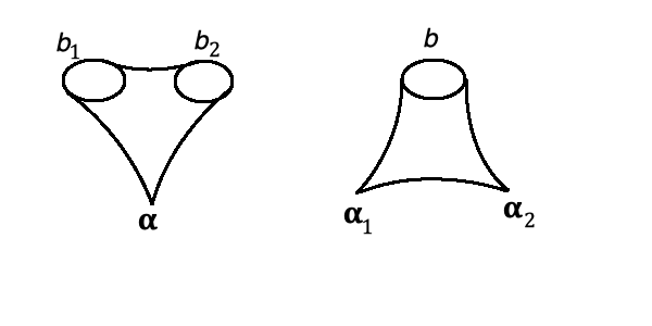
We would like to treat hyperbolic Riemann surfaces with conical singularities similarly. In this case, in addition to the trumpet and the three-holed sphere, we have to allow two more basic building blocks, which are obtained by replacing one or two of the geodesic boundaries of a three-holed sphere with conical singularities. See fig. 4.⁴⁴ 4 We do not add a sphere with three conical singularities as an additional building block because, as it has no boundary, it cannot be used in any further gluing. But because the sphere with three conical singularities cannot be made from the other building blocks, it is an exceptional case in many statements. For example, that is why, when we discuss a specific example in section 3, we will consider a sphere with four conical singularities, to which the general theory applies. As a typical example of decomposing a surface with conical singularities into these more general elementary building blocks, let us consider a surface $\Sigma$ that is a disc with an asymptotically AdS boundary and two conical singularities (fig. 3(b)). In other words, we replace the geodesic boundaries $B_{1},B_{2}$ in fig. 3(a) with conical singularities $p_{1}$, $p_{2}$ in fig 3(b). Now we try to again decompose $\Sigma$ into elementary building blocks by minimizing the length of a loop that is homologous to the outer boundary $C$. More specifically, we want to minimize the length of this loop without letting it jump across or pass through any of the conical singularities. If the minimizer exists, as sketched in fig. 3(b), we get the desired decomposition: the building blocks are now a trumpet and a sphere with one hole with geodesic boundary (namely $\gamma$) and two conical singularities ($p_{1}$ and $p_{2}$). We will use such decompositions many times in our computations.

However, in general this process will only work if, when we try to minimize the length of a loop, that loop is “repelled” from any conical singularities. If in the minimizing process, a curve gets pulled across a conical singularity, we will not get the desired decomposition. As an example to show that a nontrivial condition is needed, consider a disc with two conical singularities, as in fig. 3(b), but now assume that the two deficit angles are very small. In this case, the geometry of the disc is almost the same as that of a disc in ${\mathrm{AdS}}_{2}$. In ${\mathrm{AdS}}_{2}$, there are no closed geodesics, and adding conical singularities with very small deficit angle does not bring closed geodesics into existence. If we start with a loop homologous to $C$ and try to minimize its length, it will just jump across the conical singularities and shrink to a point. So the deficit angles must be sufficiently large to generate the decomposition sketched in fig. 3(b).

In fact, the necessary condition to ensure that the desired minimizers always exist is that the deficit angles should be all greater than $\pi$. The reason is illustrated in fig. 5. Consider two points $s_{1},s_{2}\in\Sigma$. Suppose that we are given a simple curve⁵⁵ 5 A simple curve is a curve that does not intersect itself. If a path $\gamma$ from $s_{1}$ to $s_{2}$ intersects itself at a point $p$, then by dropping from $\gamma$ a closed loop, we get a shorter path from $s_{1}$ to $s_{2}$. So in looking for length-minimizing curves, it is reasonable to consider simple curves. between $s_{1}$ and $s_{2}$ in the smooth part of $\Sigma$, and we want to shorten this curve to a geodesic. Consider first fig. 5(a). Here we illustrate a conical singularity with a deficit angle greater than $\pi$. When one tries to minimize the length of a curve between given points $s_{1}$, $s_{2}$, it is “repelled” from the singularity, in the sense that any curve from $s_{1}$ to $s_{2}$ can be shortened to turn it into a geodesic without pulling it across the conical singularity at $p$. One can specify at will which way a simple curve from $s_{1}$ to $s_{2}$ should go around $p$, and a minimizing geodesic with that property will exist.

That is not true for a conical singularity with deficit angle less than $\pi$ (fig. 5(b)). To shorten the indicated curve from $s_{1}$ to $s_{2}$, one would have to pull this curve across $p$, and one would end up with a geodesic that goes around $p$ on the other side.

We have here described the case of curves with specified endpoints, but the case we actually need of closed loops is similar. The reason for this is that whether a curve is attracted to or repelled from a conical singularity $p$ when we try to minimize its length depends only on local considerations near $p$, not on global properties of the curve.

In short, the techniques that we will use in this article to analyze the perturbation $2\varepsilon\exp(-\alpha\phi)$ will only be valid in the range $\pi<\alpha<2\pi$. However, the results that we will get will be analytic in $\alpha$, suggesting that they are valid outside the range that we start in (perhaps even for negative⁶⁶ 6 What happens for negative $\alpha$ is that the high energy behavior of the eigenvalue distribution of the dual matrix model no longer coincides with that of JT gravity. But a matrix model with that distribution does exist, as long as the sign of the coupling $\varepsilon$ is chosen so that the distribution is positive. $\alpha$). More generally, by the same methods we will be able to analyze a linear combination of such exponentials,

The result that we will get for the eigenvalue density of a dual matrix model can be expressed in a way that makes sense for a much larger class of functions, so it probably is valid in more generality than the derivation.

Volumes of moduli spaces of Riemann surfaces with conical singularities, for the case of deficit angles greater than $\pi$, have been analyzed in [28]. Understanding how this was done is important background for the problem that we will be studying.

First of all, let us compare conical singularities to holes with geodesic boundary. We recall that a hyperbolic Riemann surface $\Sigma$ has a natural flat $\mathrm{PSL}(2,{\mathbb{R}})$ connection. It is convenient to lift the holonomies to ${\mathrm{SL}}(2,R)$ and describe them as $2\times 2$ matrices of determinant 1, but this involves an arbitrary choice of sign. The holonomy around a geodesic of length $b$ is conjugate (up to sign) to

What is the holonomy around a conical singularity with deficit angle $\alpha$? In going around the conical singularity, a tangent vector is rotated by an angle $\alpha$. But ${\mathrm{SL}}(2,{\mathbb{R}})$ acts on the spin bundle, and the rotation of a spinor is by an angle $\alpha/2$. So, taking $\begin{pmatrix}0&1\cr-1&0\end{pmatrix}$ as the rotation generator, the monodromy of the flat connection around a conical singularity with deficit angle $\alpha$ is

We see that $U_{b}$ and $V_{\alpha}$ are conjugate in ${\mathrm{SL}}(2,{\mathbb{C}})$ (up to sign) if we identify $b$ with ${\mathrm{i}}(2\pi-\alpha)$. In other words, at least from the point of view of the monodromy, a conical singularity can be viewed as the analytic continuation of a hole with geodesic boundary.

From what we have said so far, it is not obvious why $b$ should be identified with $\pm{\mathrm{i}}(2\pi-\alpha)$ and not just $\pm{\mathrm{i}}\alpha$. Probably the most direct way to understand this is the following. In the limit $b\to 0$, a geodesic boundary of length $b$ reduces to a puncture, which in the context of hyperbolic geometry means a cusp. Likewise, in the limit that $\alpha$ approaches $2\pi$, a conical singularity with a deficit angle of $2\pi$ approaches a cusp. So $b=0$ corresponds to $\alpha=2\pi$, not $\alpha=0$. Note that in the limit $\alpha\to 0$, a conical singularity becomes a smooth point, not a cusp. We will see in many other ways the importance of including the $2\pi$ in the relation between $b$ and $\alpha$.

We will now make a small aside and explain something that is important in a theory with fermions but not in a purely bosonic theory such as JT gravity. A comparison between conical singularities and geodesic boundaries that does include the signs of the holonomies can be made if we pick a spin structure, in which case the holonomies become well-defined in ${\mathrm{SL}}(2,{\mathbb{R}})$. The generalization of eqn. (3.1) is then $U_{b}=\eta\exp\begin{pmatrix}b/2&0\cr 0&-b/2\end{pmatrix}$, where $\eta=-1$ for Neveu-Schwarz (NS) spin structure on the geodesic circle, and $+1$ for Ramond (R) spin structure. We then see that $V_{\alpha}$ is conjugate in ${\mathrm{SL}}(2,{\mathbb{C}})$ to the analytic continuation of $U_{b}$ if the spin structure on the geodesic is of NS type. Here it is important that $b=\pm{\mathrm{i}}(2\pi-\alpha)$, not $\pm{\mathrm{i}}\alpha$. If the spin structure of the geodesic is of R type, we need an extra minus sign in $V_{\alpha}$, which means that the conical singularity should be a Ramond singularity, producing an extra minus sign for fermions.

This relationship between conical singularities and geodesic boundaries has been important in understanding Weil-Petersson volumes in the presence of conical singularities. Mirzakhani [27] developed a technique to compute volumes of moduli spaces of hyperbolic Riemann surfaces, in general with geodesic boundaries. Thus in general she computed the volume of the moduli space ${\mathcal{M}}_{g,\vec{b}}$ of hyperbolic Riemann surfaces of genus $g$ with geodesic boundaries of lengths $\vec{b}=(b_{1},b_{2},\cdots,b_{n})$. One important ingredient in her work was the fact that a hyperbolic Riemann surface, possibly with geodesic boundaries, can be constructed (in many ways) by gluing together three-holed spheres along geodesic boundaries. In [28], it was shown that all the facts used by Mirzakhani have analogs for surfaces that have conical singularities in addition to (or instead of) geodesic boundaries, as long as all the conical singularities have deficit angles in the range⁷⁷ 7 In their terminology, the cone angle should be less than $\pi$; what they call the cone angle is the opening angle $2\pi-\alpha$ at a conical singularity, where $\alpha$ is the deficit angle. $\pi<\alpha<2\pi$. The restriction to $\alpha>\pi$ was needed because of the phenomenon that we explained in discussing fig. 5: the decomposition of a surface with conical singularities in elementary building blocks works the same way as for a surface with geodesic boundaries if and only if the deficit angles satisfy $\pi<\alpha<2\pi$. The elementary building blocks that one has to allow are familiar from section 2:⁸⁸ 8 If one wants asymptotically AdS boundaries – as we will – one adds the trumpet as another building block. a three-holed sphere; a sphere with two holes and one conical singularity; and a sphere with one hole and two conical singularities.⁹⁹ 9 A sphere with precisely three conical singularities is an exceptional case because it cannot be constructed from the usual building blocks, as noted in footnote 4. As a result, in this particular example, the condition $\alpha_{i}>\pi$ actually does not suffice for establishing a relationship between Weil-Petersson volumes for surfaces with conical singularities and Weil-Petersson volumes for surfaces with holes. A necessary and sufficient condition is that the moduli space ${\mathcal{M}}_{0,\vec{\alpha}}$ should be non-empty. It then consists of a single point and has the same volume – namely 1 – as the moduli space for a three-holed sphere, which also consists of a single point. More specifically, it was shown in [28] that as long as deficit angles are in the favored range, volumes of moduli spaces of hyperbolic surfaces with conical singularities can be obtained from the volumes of hyperbolic surfaces with geodesic boundaries by the analytic continuation $b\to{\mathrm{i}}(2\pi-\alpha)$. This consequence of their results is stated in the Additional Remark at the end of the introduction of their paper. See also [33] for some further developments.

The formulas obtained in [28] – like the formulas that we will obtain in the rest of the present paper – are analytic in $\alpha$ and may retain some validity beyond the region $\pi<\alpha<2\pi$. However, some restriction on the $\alpha$’s is really needed. To see this, let us consider the example of a four-holed sphere with geodesic boundaries of lengths $b_{1},b_{2},b_{3},b_{4}$. The volume of the moduli space was computed by Mirzakhani and is

By the result of [28], if we make a replacement $b_{i}\to{\mathrm{i}}(2\pi-\alpha_{i})$ for some (or all) of the $b_{i}$, the same formula gives the volume of the moduli space of hyperbolic metrics on a sphere with $p$ holes with geodesic boundary and $q$ conical singularities, with $p+q=4$, as long as the deficit angles are in the favored range $\pi<\alpha_{i}<2\pi$.

However, the formula is not valid in general outside of this range. For example, for $p=0$, $q=4$, the Gauss-Bonnet theorem gives a formula

where the integral is taken on the smooth part of $S^{2}$. This formula cannot be satisfied by a hyperbolic metric (which has $R<0$ away from the conical singularities) if $\sum_{i=1}^{4}\alpha_{i}\leq 4\pi$. So the moduli space of hyperbolic metrics on a sphere with the specified conical singularities is empty unless $\sum_{i=1}^{4}\alpha_{i}>4\pi$. The condition $\alpha_{i}>\pi$ that is needed for the theorem of [28] to hold ensures that $\sum_{i=1}^{4}\alpha_{i}>4\pi$. The moduli space is then nonempty and according to the result of [28], its volume is $2\pi^{2}-\frac{1}{2}\sum_{i=1}^{4}(2\pi-\alpha_{i})^{2}$.

Mirzakhani also found a formula expressing the Weil-Petersson volume $V_{g,\vec{b}}$ of ${\mathcal{M}}_{g,\vec{b}}$ in terms of an integral over ${\mathcal{M}}_{g,n}$, the moduli space of Riemann surfaces with $n$ punctures. Topologically, ${\mathcal{M}}_{g,\vec{b}}$ and ${\mathcal{M}}_{g,n}$ are equivalent, as explained for example in [25]. But the corresponding Weil-Petersson forms $\omega_{g,\vec{b}}$ and $\omega_{g,n}$ are not cohomologous. The relation between them involves the following. If $p$ is a point in a Riemann surface $\Sigma$, then the cotangent bundle to $\Sigma$ at $p$ is a one-dimensional complex vector space. As the moduli of $\Sigma$ vary, this vector space varies as the fiber of a complex line bundle ${\mathcal{L}}$ over the modulli space of Riemann surfaces. In the case of ${\mathcal{M}}_{g,n}$, there are $n$ punctures $p_{1},\cdots,p_{n}$, and therefore this construction gives $n$ complex line bundles ${\mathcal{L}}_{1},{\mathcal{L}}_{2},\cdots,{\mathcal{L}}_{n}$. Each of these line bundles has a first Chern class; we define $\psi_{i}=c_{1}({\mathcal{L}}_{i})$. Mirzakhani found the relationship between $\omega_{g,\vec{b}}$ and $\omega_{g,n}$:

This relation between symplectic forms immediately leads to a statement about volumes:¹⁰¹⁰ 10 Here $\overline{{\mathcal{M}}}_{g,n}$ is the Deligne-Mumford compactification of ${\mathcal{M}}_{g,n}$. Actually, in hyperbolic geometry, the cohomology classes have natural representatives that vanish at infinity. If one uses those representatives, one can just integrate over ${\mathcal{M}}_{g,n}$ rather than its compactification. Note that even after the compactification to $\overline{{\mathcal{M}}}_{g,n}$, punctures never collide so questions about contact terms do not arise.

Since the $\psi_{i}$ are two-dimensional classes, the integral on the right hand side is manifestly a polynomial in the variables $b_{i}^{2}$, of degree $3g-3+n$ (the complex dimension of ${\mathcal{M}}_{g,n}$). The bottom term in this polynomial, obtained by setting all $b_{i}$ to zero, is the Weil-Petersson volume of ${\mathcal{M}}_{g,n}$, and the top degree terms, which are what we get if we drop $\omega_{g,n}$ from the exponent on the right hand side of eqn. (3.6), are the correlation functions of two-dimensional topological gravity, in the sense of [24]. These are defined as

It was shown in [28] that the same formulas hold under the substitution $b\to{\mathrm{i}}(2\pi-\alpha)$ if we replace some or all of the geodesic boundaries with conical singularities in the preferred range ($\pi<\alpha<2\pi$). Thus, if ${\mathcal{M}}_{g,\vec{b},\vec{\alpha}}$ is the moduli space of hyperbolic Riemann surfaces of genus $g$ with geodesic boundaries of lengths $\vec{b}=(b_{1},b_{2},\cdots,b_{m})$ and conical singularities with deficit angles $\vec{\alpha}=(\alpha_{1},\alpha_{2},\cdots,\alpha_{n})$, then the volume $V_{g,\vec{b},\vec{\alpha}}$ is

We have denoted the $\psi$ classes associated to the holes as $\psi_{i},\,i=1,\cdots,m$, and those associated to the conical singularities as $\widetilde{\psi}_{j}$, $j=1,\cdots,n$. If $\vec{b}=0$ and all $\alpha_{j}$ are equal to $2\pi$, then ${\mathcal{M}}_{g,\vec{b},\vec{\alpha}}$ reduces to ${\mathcal{M}}_{g,n+m}$ and $V_{g,\vec{b},\vec{\alpha}}$ reduces to the volume of ${\mathcal{M}}_{g,n+m}$, which is $\int_{\overline{{\mathcal{M}}}_{g+n}}e^{\omega_{g,n+m}}$.

Before proceeding to analyze how the perturbation $U=2{\varepsilon}\exp(-\alpha\phi)$ affects the eigenvalue distribution of the matrix model, we need one more step.

An important ingredient in [3] is the evaluation of the Schwarzian path integral in two special cases: a disc with nearly ${\mathrm{AdS}}_{2}$ boundary, and a trumpet, which is the same as an annulus with one nearly ${\mathrm{AdS}}_{2}$ boundary and one geodesic boundary. To study JT gravity with conical singularities, a third example is very important. This is a disc with nearly ${\mathrm{AdS}}_{2}$ boundary and a single conical singularity.

The Schwarzian action arises in this context as the action of JT gravity, including the Gibbons-Hawking-York surface term, in a cutoff version of a spacetime that is asymptotic to ${\mathrm{AdS}}_{2}$ [29]. The resulting path integral is the exponential of the classical action times a one-loop determinant. There are no higher corrections, as the Schwarzian path integral is one-loop exact [31].

Let us first first review the calculation of the Schwarzian path integral for a disc $D$, which in this context is simply ${\mathrm{AdS}}_{2}$ itself with a cutoff at large distances. The bulk action $I_{\mathrm{JT}}$ of eqn. (1.1) vanishes on-shell, since the classical equation of motion for $\phi$ gives $R+2=0$. However, this bulk action requires a Gibbons-Hawking-York boundary term, which is

where $h$ is the induced metric of the boundary and $K$ is its extrinsic curvature. Using here $K-1$ rather than $K$ is not important for getting a well-defined variational problem and quantum theory. However, it is important for getting a theory that has a nearly ${\mathrm{AdS}}_{2}$ limit. The reason is simply that the extrinsic curvature of a disc in ${\mathrm{AdS}}$ space approaches 1 in the limit of a large disc.

As was explained in section 2, the metric of ${\mathrm{AdS}}_{2}$ is described by

and the usual boundary conditions for a large disc embedded in ${\mathrm{AdS}}_{2}$ are satisfied by the disc $D$ defined by $\rho\leq\rho_{0}$, with the dilaton

where $\beta$ is the renormalized circumference of $D$. To evaluate the GHY surface term in this situation, we note that the boundary of $D$ has circumference $L=2\pi\sinh\rho_{0}.$ For $\phi|_{\partial D}$ equal to the constant $\phi_{\mathrm{b}}$, one term in the GHY action is

The other term is proportional to the extrinsic curvature. One way to evaluate that term [32] is to use the Gauss-Bonnet theorem

where $\chi$ is the Euler characteristic. Since the disc has $\chi=1$ and ${\mathrm{AdS}}_{2}$ has $R=-2$, the right hand side of (4.5) is $2\pi+A$, where $A=2\pi(\cosh\rho_{0}-1)$ is the area of $D$. So

Finally we see that the on-shell boundary action of a disc is $-\frac{2\pi^{2}}{\beta}(\cosh^{2}\rho_{0}-\cosh\rho_{0}\sinh\rho_{0})=-\frac{\pi^{2}}{\beta}(1+e^{-2\rho_{0}})$, which in the limit $\rho_{0}\to\infty$ becomes

In the present paper, we will need the corresponding formula for what we will call $D(\alpha)$, a disc with a single conical singularity with deficit angle $\alpha$. The metric of $D(\alpha)$ can be described by the same formula (4.2), but now the range of $\psi$ is $0\leq\psi\leq 2\pi-\alpha$ rather than $0\leq\psi\leq 2\pi$. As before, we can satisfy the equation of motion for $\phi$ and the boundary conditions by taking $\phi={\mathrm{C}}\cosh\rho$ and defining $D(\alpha)$ as the region $\rho\leq\rho_{0}$. Because $\psi$ is now integrated over a smaller range, we get now $L=(2\pi-\alpha)\sinh\rho_{0}$ and $\int_{\partial D(\alpha)}\mathrm{d}x\sqrt{h}K=(2\pi-\alpha)\cosh\rho_{0}$. So (4.7) is replaced by $I_{D(\alpha)}=-(2\pi-\alpha){\mathrm{C}}/2$. The formula for the renormalized circumference $\beta$ becomes $\beta=\lim_{\rho_{0}\to\infty}L/2\phi_{\mathrm{b}}=(2\pi-\alpha)/2{\mathrm{C}}$, so in terms of $\beta$, we get

We will also need the corresponding formula for the trumpet, so let us recall how it is derived. For the metric of a trumpet $T(b)$, we can take

Here $\rho$ ranges over $0\leq\rho\leq\rho_{0}$, with a cutoff at very large $\rho_{0}$. The boundary at $\rho=0$ is a geodesic of circumference $b$. The equation of motion for the dilaton can be solved by $\phi={\mathrm{C}}\sinh\rho$. Imposing that $\phi$ restricted to the boundary should be a constant $\phi_{\mathrm{b}}$, we get $\phi_{\mathrm{b}}={\mathrm{C}}\sinh\rho_{0}$. Imposing that the circumference should be $L$, we get $L=b\cosh\rho_{0}$. Evaluating $\int_{\partial T}\mathrm{d}x\sqrt{h}K$ as $2\pi\chi+A$, where $A$ is the area of $T$ and now $\chi=0$, we get $\int_{\partial T}\mathrm{d}x\sqrt{h}K=b\sinh\rho_{0}$. Hence the action of the trumpet is $I_{T}=\phi_{\mathrm{b}}(L-A)={\mathrm{C}}\sinh\rho_{0}(b\cosh\rho_{0}-b\sinh\rho_{0})=\frac{b{\mathrm{C}}}{2}(1-e^{-2\rho_{0}})$. Taking $\rho_{0}\to\infty$ and defining $\beta=\lim_{\rho_{0}\to\infty}L/2\phi_{\mathrm{b}}=b/2{\mathrm{C}}$, we get

Comparing eqns. (4.8) and (4.10), we see that the classical actions for $T(b)$ and $D(\alpha)$ are related by $b\to{\mathrm{i}}(2\pi-\alpha)$, though the derivation did not make it obvious that this would be so.

The Schwarzian path integral is the exponential of the classical action times a one-loop determinant. A localization argument shows that there are no higher order corrections [31]. The Schwarzian modes for $D$ parametrize ${\mathrm{diff}}\,S^{1}/{\mathrm{PSL}}(2,{\mathbb{R}})$, but the Schwarzian modes for $D(\alpha)$ and $T$ both parametrize ${\mathrm{diff}}\,S^{1}/{\mathrm{U}}(1)$. This plus the localization procedure implies that the one-loop determinants for $D(\alpha)$ and $T(b)$ are the same (and moreover independent of $\alpha$ and $b$).¹¹¹¹ 11 In the localization procedure of Duistermaat and Heckman (and Atiyah and Bott) which was exploited in [31], one considers an action of the group ${\mathrm{U}}(1)$ on a symplectic manifold $M$, with symplectic form $\omega$ and Hamiltonian $H$. One then considers the integral $\int_{M}\exp(H/\beta+\omega)$. In general in this situation, the one-loop determinant in expanding around a fixed point $p$ of the ${\mathrm{U}}(1)$ action depends only on the “rotation angles” with which the group ${\mathrm{U}}(1)$ acts on the tangent space to $M$ at $p$. It does not depend on $H$ or $\omega$. In our application, the relevant ${\mathrm{U}}(1)$ group is the group of rotations of the asymptotically AdS boundary of the two-dimensional surface. $D(\alpha)$ and $T(b)$ have different $H$ and $\omega$, but as spaces they are the same homogeneous space ${\mathrm{diff}}\,S^{1}/{\mathrm{U}}(1)$ with the same ${\mathrm{U}}(1)$ action, so they have the same one-loop determinants. We can therefore borrow the results for the determinants from eqn. (7) of [3] (where we set $\gamma=1/2$ as remarked in footnote 3). So the Schwarzian path integrals for the three examples are

The JT gravity path integrals for the three examples differ from these expressions only by an additional factor $e^{\chi{\sf S}_{0}}$ coming from the Einstein-Hilbert action; here $\chi$ is the Euler characteristic and ${\sf S}_{0}$ is the ground state entropy. Note that $\chi=1$ for $D$ and $D(\alpha)$ and $\chi=0$ for $T(b)$.

It is now straightforward to compute the first order effect of a perturbation $U(\phi)$ on the eigenvalue density $\rho(E;U)$ of a hypothetical dual matrix model.

The basic idea is that the partition function $Z_{D}(\beta;U)$ of the bulk theory on a disc with asymptotically AdS boundary is interpreted as $Z_{D}(\beta;U)=\int_{E_{0}}^{\infty}\mathrm{d}E\,e^{-\beta E}\rho(E;U)$, where $E_{0}$ is the threshold energy and $\rho(E;U)$ is the density of eigenvalues. In the present case, the disc may contain any number of conical singularities of deficit angle $\alpha$, each coming with a factor $\varepsilon$. The first two terms are the JT gravity path integrals on $D$ and $D(\alpha)$:

We included a factor $e^{{\sf S}_{0}}$ from the Einstein-Hilbert action.

To put $Z_{D}(\beta;U)$ in the form $\int_{E_{0}}^{\infty}\mathrm{d}E\,e^{-\beta E}\rho(E;U)$ is an exercise in Gaussian integrals. Using

we learn, after setting $E=\phi^{2}$, that

References

- [1] R. Jackiw, “Lower Dimensional Gravity,” Nucl. Phys. B252 (1985) 343-56.
- [2] C. Teitelboim, “Gravitation and Hamiltonian Structure in Two Space-Time Dimensions,” Phys. Lett. B126 (1983) 41Ð5.
- [3] P. Saad, S. Shenker, and D. Stanford, “JT Gravity As A Matrix Integral,” arXiv:1903.11115.
- [4] T. Banks and M. O’Loughlin, “Two-Dimensional Quantum Gravity In Minkowski Space,” Nucl. Phys. B362 (1991) 649-64.
- [5] D. Louis-Martinez, J. Gegenberg, and G. Kunstatter, “Exact Quantization of All Dilaton Gravity Theories,” Phys. Lett. B321 (1994) 193-8, arXiv:gr-qc/0309018.
- [6] N. Ikeda, “Two-Dimensional Gravity and Nonlinear Gauge Theory,” Ann. Phys. 235 (1994) 435-64, arXiv:hep-th/9312059.
- [7] D. Weingarten, “Euclidean Quantum Gravity On A Lattice,” Nucl. Phys. B210 [FS6] (1982) 229.
- [8] V. Kazakov, “Bilocal Regularization Of Models Of Random Surfaces,” Phys. Lett. 150B (1985) 282.
- [9] F. David, “Randomly Triangulated Surfaces In Two Dimensions,” Nucl. Phys. B257 [FS14] (1985) 45.
- [10] J. Ambjorn, B. Durhuus, and J. Frohlich, “Diseases of Triangulated Random Surfaces, and Possible Cures,” Nucl. Phys. B257 [FS14] (1985) 433.
- [11] V. Kazakov, I. Kostov, and A. Migdal, “Critical Properties Of Randomly Triangulated Planar Random Surfaces,” Phys. Lett. 157B (1985) 295.
- [12] E. Brézin and V. Kazakov, “Exactly Solvable Field Theories Of Closed Strings,” Phys. Lett. B236 (1990) 144.
- [13] M. Douglas and S. Shenker, “Strings In Less Than One Dimension,” Nucl. Phys. B335 635 (1990).
- [14] D. J. Gross and A. Migdal, “Nonperturbative Two-Dimensional Quantum Gravity,” Phys. Rev. Lett. 64 (1990) 127.
- [15] P. Ginsparg and G. Moore, “Lectures on 2D Gravity And 2D String Theory,” hep-th/9304011.
- [16] P. Di Francesco, P. H. Ginsparg, and J. Zinn-Justin, “2-D Gravity and Random Matrices,” Phys. Rept. 254 (1995) 1-133.
- [17] E. Brézin, C. Itzykson, G. Parisi, and J.-B. Zuber, “Planar Diagrams,” Comm. Math. Phys. 59 (1978) 35-51.
- [18] D. Kutasov, “Geometry on the Space of Conformal Field Theories and Contact Terms,” Phys. Lett. B220 (1989) 153-8.
- [19] E. Witten, “Deformations of JT Gravity And Phase Transitions,” arXiv:2006.03494.
- [20] H. Maxfield and G. Turiaci, “The Path Integral of 3D Gravity Near Extremality, or JT Gravity WIth Defects as a Matrix Integral,” arXiv:2006.11317.
- [21] T. G. Mertens and G. Turiaci, “Defects in Jackiw-Teitelboim Quantum Gravity,” arXiv:1904.05228.
- [22] T. G. Mertens and G. Turiaci, “Liouville Quantum Gravity – Holography, JT, and Matrices,” arXiv:2006.07072.
- [23] J. Cotler, K. Jensen, and A. Maloney, “Low-dimensional de Sitter Quantum Gravity,” arXiv:1905.03780.
- [24] E. Witten, “Two-Dimensional Gravity And Intersection Theory On Moduli Space,” Surveys Diff. Geom. 1 (1991) 243-310.
- [25] R. Dijkgraaf and E. Witten, “Developments in Topological Gravity,” Int. J. Mod. Phys. A33 (2018) 1830029, arXiv:1804.03275.
- [26] B. Eynard and N. Orantin, “Weil-Petersson Volume of Moduli Spaces, Mirzakhani’s Recursion and Matrix Models,” arXiv:0705.3600.
- [27] M. Mirzakhani, “Weil-Petersson Volumes and Intersection Theory On The Moduli Space Of Curves,” Journal AMS 20 (2007) 1-23.
- [28] S. P. Tan, Y. L. Wong, and Y. Zhang, “Generalizations Of McShane’s Identity To Hyperbolic Cone-Surfaces,” J. Diff. Geom. 72 (2006) 73-112.
- [29] J. Maldacena, D. Stanford, and Z. Yang, “Conformal Symmetry And Its Breaking In Two Dimensional Nearly Anti de Sitter Space,” arXiv:1606.01857.
- [30] D. Stanford and E. Witten, “JT Gravity And The Ensembles Of Random Matrix Theory,” arXiv:1907.03363.
- [31] D. Stanford and E. Witten, “Fermionic Localization Of The Schwarzian Theory,” JHEP 10 (2017) 008, arXiv:1703.04612.
- [32] Z. Yang, “The Quantum Gravity Dynamics Of Near Extremal Black Holes,” arXiv:1809.08647.
- [33] N. Do and P. Norbury, “Weil-Petersson Volumes and Cone Surfaces,” arXiv:math/0603406.
- [34] M. F. Atiyah, “Resolution of Singularities and Division of Distributions,” Comm. Pure Appl. Math. 23 (1970) 145-50.
- [35] B. Eynard and N. Orantin, “Invariants of Algebraic Curves and Topological Expansion,” arXiv:math-ph/0702045.