Online Competitive Influence Maximization
Jinhang Zuo Xutong Liu Carlee Joe-Wong Carnegie Mellon University The Chinese University of Hong Kong Carnegie Mellon University
John C.S. Lui Wei Chen The Chinese University of Hong Kong Microsoft Research
Abstract
Online influence maximization has attracted much attention as a way to maximize influence spread through a social network while learning the values of unknown network parameters. Most previous works focus on single-item diffusion. In this paper, we introduce a new Online Competitive Influence Maximization (OCIM) problem, where two competing items (e.g., products, news stories) propagate in the same network and influence probabilities on edges are unknown. We adopt a combinatorial multi-armed bandit (CMAB) framework for OCIM, but unlike the non-competitive setting, the important monotonicity property (influence spread increases when influence probabilities on edges increase) no longer holds due to the competitive nature of propagation, which brings a significant new challenge to the problem. We provide a nontrivial proof showing that the Triggering Probability Modulated (TPM) condition for CMAB still holds in OCIM, which is instrumental for our proposed algorithms OCIM-TS and OCIM-OFU to achieve sublinear Bayesian and frequentist regret, respectively. We also design an OCIM-ETC algorithm that requires less feedback and easier offline computation, at the expense of a worse frequentist regret bound. Experimental evaluations demonstrate the effectiveness of our algorithms.
1 Introduction
Influence maximization, motivated by viral marketing applications, has been extensively studied since Kempe et al., 2003 formally defined it as a stochastic optimization problem: given a social network and a budget , how should a set of seed nodes in be chosen such that the expected number of final activated nodes under a given diffusion model is maximized? They proposed the well-known Independent Cascade (IC) and Linear Threshold (LT) diffusion models, and gave a greedy algorithm that outputs a -approximate solution for any . However, they only considered a single item (e.g., product, idea) propagating in the network. In reality, different items could propagate concurrently in the same network, interfering with each other and leading to competition during propagation. Several competitive diffusion models (Carnes et al., 2007; Bharathi et al., 2007; Budak et al., 2011; He et al., 2012; Ivanov et al., 2017) have been proposed for this setting. We use a Competitive Independent Cascade (CIC) model (Chen et al., 2013), which extends the classical IC model to multi-item influence diffusion. We consider the competitive influence maximization problem between two items from the “follower’s perspective”: given the seed nodes of the competitor’s item, the follower’s item chooses a set of nodes so as to maximize the expected number of nodes activated by the follower’s item, referred to as the influence spread of the item.
| Algorithm | No Prior? | Offline computation | Feedback | Regret |
|---|---|---|---|---|
| OCIM-TS | Standard | Full propagation | Bayes. | |
| OCIM-OFU | ✓ | Hard | Full propagation | Freq. |
| OCIM-ETC | ✓ | Standard | Direct out-edges | Freq. |
We refer to the above problem as “offline” competitive influence maximization, since the influence probabilities on edges, i.e., the probabilities of an item’s propagation along edges, are known in advance. It can be solved by a greedy algorithm due to submodularity (Chen et al., 2013). However, in many real-world applications, the influence probabilities on edges are unknown. We study the competitive influence maximization in this setting, and call it the Online Competitive Influence Maximization (OCIM) problem. In OCIM, the influence probabilities on edges need to be learned through repeated influence maximization trials: in each round, given the seed nodes of the competitor, we (i) choose seed nodes; (ii) observe the resulting diffusion that follows the CIC model to update our knowledge of the edge probabilities; and (iii) obtain a reward, which is the total number of nodes activated by our item. Our goal is to choose the seed nodes in each round based on previous observations so as to maximize the cumulative reward.
Most previous studies on the online non-competitive influence maximization problem use a combinatorial multi-armed bandit (CMAB) framework (Chen et al., 2016; Wen et al., 2017), an extension of the classical multi-armed bandit problem that captures the tradeoff between exploration and exploitation in sequential decision making. In CMAB, a player chooses a combinatorial action to play in each round, observes a set of arms triggered by this action and receives a reward. The player aims to maximize her cumulative reward over multiple rounds, navigating a tradeoff between exploring unknown actions/arms and exploiting the best known action. CMAB algorithms must also deal with an exponential number of possible combinatorial actions, which makes exploring all actions infeasible.
Our Contributions. To the best of our knowledge, we are the first to study the online competitive influence maximization problem. We introduce a general contextual combinatorial multi-armed bandit framework with probabilistically triggered arms (C2MAB-T) for OCIM. Within this framework, OCIM presents a new challenge: the key monotonicity property (influence spread increases when influence probabilities on edges increase) no longer holds due to the competitive nature of propagation, and thus upper confidence bound (UCB) based algorithms (Chen et al., 2016; Wen et al., 2017) cannot be directly applied to OCIM. Such non-monotonicity also complicates the analysis of the important Triggering Probability Modulated (TPM) condition for CMAB (Wang and Chen, 2017), and we provide a non-trivial new proof to show it still holds for OCIM. We are the first to identify the OCIM problem as a natural CMAB problem without monotonicity and tackle it from three directions, providing three solutions with different tradeoffs, as shown in Table 1: OCIM-TS uses standard offline oracles to achieve good Bayesian regret, but requires prior knowledge of edge probabilities; OCIM-OFU has a stronger frequentist regret bound without prior knowledge, but requires harder offline computation; and OCIM-ETC uses standard offline oracles and fewer observations, but leads to a worse frequentist regret bound. None is a perfect solution for OCIM, but we believe their tradeoffs shed light on the challenges involved in solving OCIM and even general CMAB problems without monotonicity. Our regret analysis of OCIM-TS delicately combines the key property of Thompson Sampling (TS) with the TPM condition to tackle non-monotonicity and allows any benchmark (exact, approximate, or even heuristic) oracle; our analysis of OCIM-OFU and OCIM-ETC extends the analysis for CMAB to a new contextual setting (C2MAB-T) where the contexts are defined as the feasible sets of super arms and are not bonded with base arms. We also discuss the extension of our framework to settings with more complex competitor actions. Experiments on two real-world datasets demonstrate the effectiveness of our proposed algorithms. Due to the space constraint, we discuss important insights of our proofs and move the complete proofs as well as the results for the general C2MAB-T problem to the Appendix.
Related Work. Kempe et al., 2003 formally defined the influence maximization problem in their seminal work. Since then, the problem has been extensively studied (Li et al., 2018). Borgs et al., 2014 presented a breakthrough approximation algorithm that runs in near-linear time, which was improved by a series of algorithms (Tang et al., 2015; Nguyen et al., 2016; Tang et al., 2018). A number of studies (Carnes et al., 2007; Bharathi et al., 2007; Budak et al., 2011; He et al., 2012; Lin and Lui, 2015; Ivanov et al., 2017) addressed competitive influence maximization problems where multiple competing sources propagate in the same network. Carnes et al., 2007 proposed the distance-based and wave propagation models, and considered the influence maximization problem from the follower’s perspective. Bharathi et al., 2007 considered the CIC model and gave an algorithm for computing the best response to an opponent’s strategy.
When the influence probabilities of edges are unknown, the non-competitive online influence maximization problem has been extensively studied (Chen et al., 2016; Wang and Chen, 2017; Wen et al., 2017; Wu et al., 2019; Vaswani et al., 2017; Perrault et al., 2020). Chen et al., 2016 studied the problem under the IC model and proposed a general CMAB framework. We introduce a new contextual extension of CMAB, called C2MAB-T, different from the contextual CMAB studied by Chen et al., 2018 and Qin et al., 2014: they consider the context features of all base arms and assume the action space of super arms is a subset of all base arms, while we consider the feasible set of super arms as the context, which is more flexible than a subset of all base arms. Wang and Chen, 2017 introduced a triggering probability modulated (TPM) bounded smoothness condition to remove an undesired factor in the regret bound of Chen et al., 2016. Perrault et al., 2020 introduced a budgeted online influence maximization framework, where marketers optimize their seed sets under a budget rather than a cardinality constraint. Our OCIM-TS algorithm is similar to the Combinatorial Thompson Sampling (CTS) algorithm of Wang and Chen, 2018. However, CTS requires an exact oracle and has frequentist regret bound, while OCIM-TS allows any benchmark oracle and has Bayesian regret bound. Hüyük and Tekin, 2020 studied the Bayesian regret of CTS for CMAB, but they also require an exact oracle and a monotonicity assumption that does not hold for OCIM. Our Bayesian regret analysis is also different from that of Russo and Van Roy, 2016: they only study a simple special CMAB problem, while we provide the regret bound for general C2MAB-T instances, including the OCIM problem.
2 OCIM Formulation
In this section we present the formulation of OCIM. We first introduce the traditional competitive influence maximization problem, and then discuss its online extension where edge probabilities are unknown.
2.1 Competitive Independent Cascade Model
We consider a Competitive Independent Cascade (CIC) model, which is an extension of the classical IC model to multi-item influence diffusion. A network is modeled as a directed graph with nodes and edges. Every edge is associated with a probability . There are two items, and , trying to propagate in from their own seed sets and . The influence propagation runs as follows: nodes in (resp. ) are activated by (resp. ) at step ; at each step , a node activated by (resp. ) in step tries to activate each of its inactive out-neighbors to be (resp. ) with an independent probability that is the same for and (i.e., we consider a homogeneous CIC model). The homogeneity assumption is reasonable since typically and are two items of the same category (thus competing), so they are likely to have similar propagation characteristics.
If two in-neighbors of activated by and respectively both successfully activate at step , then a tie-breaking rule is applied at to determine the final adoption. In this paper, we consider two types of tie-breaking rules: dominance (Budak et al., 2011) and proportional (Chen et al., 2011) tie-breaking rules. Dominance tie-breaking with (resp. ) means will always adopt (resp. ) in a competition. Proportional tie-breaking means that if there are in-neighbors activated by and in-neighbors activated by trying to activate at the same step, the probability that adopts (resp. ) is (resp. ). The same tie-breaking rule also applies to the case when a node is selected both as an -seed and a -seed. The process stops when no nodes activated at a step have inactive out-neighbors.
We consider the follower’s perspective in the optimization task: let be the follower and be the competitor. Then given , our goal is to choose at most seed nodes in as to maximize the influence spread of , denoted as , which is the expected number of nodes activated by after the propagation ends. According to Budak et al., 2011’s result, the above optimization task under the homogeneous CIC model with the dominance tie-breaking rule has the monotone and submodular properties, and thus can be approximately solved by a greedy algorithm.
2.2 OCIM Model
In the online competitive influence maximization (OCIM) problem, the edge probabilities ’s are unknown and need to be learned: in each round , given , we can choose up to seed nodes as , observe the whole propagation of and that follows the CIC model, and obtain the reward, which is the number of nodes finally activated by in this round. The propagation feedback observed is then used to update the estimates on edge probabilities ’s, so that we can achieve better influence maximization results in subsequent rounds. Our goal is to accumulate as much reward as possible through this repeated process over multiple rounds.
We introduce a new contextual combinatorial multi-armed bandit framework with probabilistically triggered arms (C2MAB-T) for the OCIM problem, which is a contextual extension of CMAB-T from Wang and Chen, 2017. In OCIM, the set of edges is the set of (base) arms , and their outcomes follow independent Bernoulli distributions with expectation for all . We denote the independent samples of arms in round as , where means the -th edge is on (or live) and means the -th edge is off (or blocked) in round , and thus corresponds to the live-edge graph (Kempe et al., 2003) in round . We consider the seed set of the competitor, , as the context in round since it is determined by the competitor and can affect our choice of . We define as the action space in round and as the real action. We define the triggered arm set as the set of edges reached by the propagation from either or . Thus, is the set of edges where can be reached from by passing through only edges with . The outcomes of for all are observed as the feedback. We denote the obtained reward in round as , which is the number of nodes finally activated by . The expected reward is a function of the action and the vector . Note that our framework can also handle dynamic tie-breaking rules over different rounds, by treating the tie-breaking rule as a part of the context. For ease of explanation, we assume a fixed tie-breaking rule in this paper.
The performance of a learning algorithm is measured by its expected regret, which is the difference in expected cumulative reward between always playing the best action and playing actions selected by algorithm . Let denote the expected reward of the optimal action in round . Since the offline influence maximization under the CIC model is NP-hard (Budak et al., 2011), we assume that there exists an offline -approximation oracle , which takes and as inputs and outputs an action such that , where is the approximation ratio and is the success probability. Instead of comparing with the exact optimal reward, we use the following -approximation frequentist regret for rounds:
| (1) |
where is the action chosen by algorithm in round . Here is the context and is the seed set of item chosen by algorithm .
Another way to measure the performance of the algorithm is using Bayesian regret (Russo and Van Roy, 2014). Denote the prior distribution of as (we will discuss how to derive for OCIM in Section 4). When the prior is given, the corresponding Bayesian regret is defined as:
| (2) |
We will design algorithms to solve the OCIM problem and bound their achieved Bayesian and frequentist regrets in Section 4 and Section 5, respectively. We also discuss the general C2MAB-T problem and its solutions in the Appendix.
3 Properties of OCIM
In this section, we first show that the key monotonicity property for CMAB does not hold in OCIM. We then prove that the important Triggering Probability Modulated (TPM) condition still holds, which is essential for the analysis of all proposed algorithms.
3.1 Non-monotonicity
The monotonicity condition given by Wang and Chen, 2017 could be stated as follows in the context of OCIM: for any action , for any two expectation vectors and , we have if for all . Figure 1 shows a simple example of OCIM that does not satisfy the monotonicity condition. The left and right nodes are the seed nodes of and ; the numbers below edges are influence probabilities. It is easy to calculate that , for both dominance and proportional tie-breaking rules. Thus, if we increase , will decrease, which is contrary to monotonicity. In general, for every edge , depending on the positions of the - and -seeds, increasing the influence probability of may benefit the propagation of or may benefit the propagation of and thus impair the propagation of . Thus, the influence spread of has intricate connections with the influence probabilities on the edges.

The lack of monotonicity poses a significant challenge to the OCIM problem. We cannot directly use UCB-type algorithms (Chen et al., 2016), as they will not provide optimistic solutions to bound the regret.
3.2 Triggering Probability Modulated (TPM) Bounded Smoothness
The lack of monotonicity further complicates the analysis of the Triggering Probability Modulated (TPM) condition (Wang and Chen, 2017), which is crucial in establishing regret bounds for CMAB algorithms. We use to denote the probability that the action triggers arm when the expectation vector is . The TPM condition in OCIM is given below.
Condition 1.
(1-Norm TPM bounded smoothness). We say that an OCIM problem instance satisfies 1-norm TPM bounded smoothness, if there exists (referred to as the bounded smoothness coefficient) such that, for any two expectation vectors and , and any action , we have .
Fortunately, with a more intricate analysis, we are able to show the following TPM condition.
Theorem 3.1.
Under both dominance and proportional tie-breaking rules, OCIM instances satisfy the 1-norm TPM bounded smoothness condition with coefficient , where is the maximum number of nodes that any one node can reach in graph .
The proof of the above theorem is one of the key technical contributions of the paper. In the non-competitive setting, an edge coupling method could give a relatively simple proof for the TPM condition.11 1 The original proof in (Wang and Chen, 2017) occupies several pages, but Li et al., 2020 (in their Appendix E) provide a much shorter proof based on edge coupling. The idea of edge coupling is that for every edge , we sample a real number uniformly at random, and determine to be live under if and blocked if , and similarly for . This couples the live-edge graphs and under and respectively. In the non-competitive setting, due to the monotonicity property, we only need to consider the TPM condition when (coordinate-wise), and this implies that is a subgraph of , which significantly simplifies the analysis. However, in the competitive setting, monotonicity does not hold, and we have to show the TPM condition for every pair of and . Thus, and no longer have the subgraph relationship. In this case, we have to show that for every coupling and , for every that is activated by in but not activated by in , it is because either (a) some edge is live in but blocked in while is -activated (or equivalently is -triggered); or (b) some edge is live in but blocked in while is -triggered. The case (b) is due to the possibility of blocking ’s propagation, a unique scenario in OCIM. The above claim needs nontrivial inductive proofs for dominance and proportional tie-breaking rules, and then its correctness ensures the TPM condition.
4 Bayesian Regret Approach
In our OCIM model, since the samples of base arms follow Bernoulli distributions with mean vector , we can assume the prior distributions of , , are Beta distributions, where for all arm . Given the prior distributions of all arms, we propose an Online Competitive Influence Maximization-Thompson Sampling (OCIM-TS) algorithm, which is described in Algorithm 1. We initialize the prior distribution of each arm to . Then we take the context and the sampled from prior distributions as inputs to the oracle , and get an output action . After taking this action, we get feedback ’s from all triggered arms , then use them to update the prior distributions of all triggered base arms in .
Let be the set of arms that can be triggered by . We define as the largest number of arms that could be triggered by a feasible action. We provide the Bayesian regret bound of OCIM-TS.
Theorem 4.1.
The OCIM-TS algorithm has the following Bayesian regret bound with as defined in Theorem 3.1:
| (3) |
This regret bound essentially matches the distribution-independent frequentist regret bound of OCIM-OFU in the next section. The proof of the above theorem is inspired by the posterior sampling regret decomposition of Russo and Van Roy, 2014. However, we combine the key property of posterior sampling with the TPM condition in Theorem 3.1 to tackle non-monotonicity. OCIM-TS can also be applied to general C2MAB-T problems and allows any benchmark offline oracles (e.g., approximate or heuristic oracles). We provide the Bayesian regret bound of OCIM-TS on general C2MAB-T problems in the Appendix.
5 Frequentist Regret Approach
Although OCIM-TS can solve the OCIM problem with a standard offline oracle (e.g., TCIM in Lin and Lui, 2015), it requires the prior distribution of the network parameter , which might not be available in practice. In this section, we first propose the OCIM-OFU algorithm. It achieves good frequentist regret without the prior knowledge, but requires a new oracle to solve a harder offline problem. We then design the OCIM-ETC algorithm, which requires less feedback and easier offline computation, but yields a worse frequentist regret bound.
5.1 OCIM-OFU Algorithm
As discussed in Section 3.1, due to the lack of monotonicity, we cannot directly use UCB-type algorithms. However, it is still possible to design bandit algorithms following the principle of Optimism in the Face of Uncertainty (OFU). We first introduce a new offline problem that jointly optimizes for both the seed set and the optimal influence probability vector , where each dimension of , , is searched within a confidence interval , for all .
| (4) | ||||||
We then define a new offline -approximation oracle to solve this problem. Oracle takes and ’s as inputs and outputs and action , such that , where is the optimal solution for Eq.(4).
With the offline oracle , we propose an algorithm following the principle of Optimism in the Face of Uncertainty (OFU), named OCIM-OFU. The algorithm maintains the empirical mean and confidence radius for each edge probability. It uses the lower and upper confidence bounds to determine the range of : , where we use and to denote and for any real number . It feeds and all current ’s into the offline oracle to obtain the action to play at round . The confidence radius is large if arm is not triggered often, which leads to a wider search space to find the optimistic estimate of . We provide its frequentist regret bound.
Theorem 5.1.
The OCIM-OFU algorithm has the following distribution-independent bound (see the Appendix for the distribution-dependent bound) with defined in Theorem 3.1 ,
The above regret bound has the typical form of , indicating that it is tight on the important time horizon . In fact, it has the same order as in Wang and Chen, 2017’s for the CMAB problem under monotonicity, despite the fact that the OCIM problem does not enjoy monotonicity, and matches the lower bound of CMAB with general reward functions in (Merlis and Mannor, 2020). This result is due to our non-trivial TPM condition analysis (Theorem 3.1) that shows the same condition as in Wang and Chen, 2017’s setting with monotonicity.
Computational Efficiency. We now discuss the computational complexity of implementing the OCIM-OFU algorithm. We show the complexity of the new offline optimization problem in Eq. (4).
Theorem 5.2.
The offline problem in Eq.(4) is #P-hard.
As mentioned before, the original offline problem, i.e., maximizing over when fixing , can be solved by several algorithms (Lin and Lui, 2015) based on submodularity of over . A straightforward attempt on the new offline problem in Eq.(4) is to show the submodularity of over , and then to use a greedy algorithm on to select . Unfortunately, we find that is not submodular (see the Appendix for a counterexample). Implementing the oracle is then a challenge. However, it is possible to design efficient approximate oracles for bipartite graphs, which model the competitive probabilistic maximum coverage problem with applications in online advertising (Chen et al., 2016). The main idea is that we can pre-determine that either the lower or the upper bound of is optimal and should be chosen as depending on the tie-breaking rule, then use existing efficient influence maximization algorithms to get approximate solutions. The competitive propagation in the general graph is much more complicated, but we have a key observation that the optimal solution for the optimization problem in Eq.(4) must occur at the boundaries of the intervals . Based on that, we discuss solutions for some specific graphs such as trees. See the Appendix for more details.
5.2 OCIM-ETC Algorithm
In this section, we propose an OCIM Explore-Then-Commit (OCIM-ETC) algorithm. It has two advantages: first, it does not need the new offline oracle discussed in Sec. 5.1; and second, it requires fewer observations than our other algorithms: instead of the observations of all triggered edges, i.e., , it only needs the observations of all direct out-edges of seed nodes.
Like other ETC algorithms (Garivier et al., 2016), OCIM-ETC divides the rounds into two phases: an exploration phase and an exploitation phase. In the exploration phase, it chooses each node as the seed node of for times. The exploration phase thus takes rounds. In the exploitation phase, it takes and the empirical means as inputs to the oracle mentioned in Sec. 2, then plays the output action . We give its frequentist regret bound.
Theorem 5.3.
The OCIM-ETC algorithm has the following distribution-independent regret bound (see the Appendix for the distribution-dependent bound) with defined in Theorem 3.1, when ,
| (5) |
Although this regret bound is worse than that of the OCIM-OFU algorithm in Theorem 5.1, OCIM-ETC requires easier offline computation and less feedback since it only needs to observe the results of direct out-edges of seed nodes, which shows the tradeoff between regret bound and feedback/computation in OCIM.
6 Extension to Probabilistic Seed Distribution for the Competitor
Lin and Lui, 2015 extend the offline CIM problem to a probabilistic setting where the competitor’s seed distribution is known (i.e., the probability of each node being selected as a seed by the competitor). In this section, we extend our algorithms to handle two new settings where the competitor has a probabilistic seed distribution. Note that we need to slightly modify the TPM condition for these settings. We denote the expected reward of follower as , where is the seed set of , is the seed distribution of . We use to denote the probability that either or will trigger arm when the seed set of is , the seed set of , , is sampled from , and the expectation vector is . The modified TPM condition is given below.
Condition 2.
(Modified TPM bounded smoothness). We say that an OCIM problem instance satisfies modified TPM bounded smoothness, if there exists such that, for any two expectation vectors and , and any seed set and seed distribution , we have .
With the similar analysis of Theorem 3.1, we can show the following TPM condition when the competitor has probabilistic seed distribution.
Theorem 6.1.
Under both dominance and proportional tie-breaking rules, OCIM instances satisfy the modified TPM bounded smoothness condition with coefficient , where is the maximum number of nodes that any one node can reach in graph .
Known dynamic seed distribution. In round , the competitor’s seed set follows a distribution , i.e., . However, the follower only knows but not before choosing . Since our proposed framework has a nice separation between online learning and offline computation, in this setting, only the offline computation part will be affected. Specifically, we can replace the oracle in OCIM-TS and OCIM-ETC with a new oracle . For OCIM-OFU, similar to oracle , we need a new oracle that takes and the confidence intervals as inputs and outputs . We can use the TCIM algorithm of (Lin and Lui, 2015) to design and . Our proposed algorithms will have the same regret bounds as in Theorems 4.1 and 5.1.
Unknown fixed seed distribution. In this setting, the seed distribution of the competitor, , is unknown to the follower but fixed for all rounds. To solve this problem, we introduce a virtual seed node , which connects to each existing node with an unknown edge probability equal to the probability of being selected as a seed. This reduces the case of probabilistic seed selection to the standard CIC model with a known seed node . The unknown edge probabilities ’s can be learned together with the edge probabilities in the original graph. Therefore, we do not need to know the competitor’s seed selection in advance and can learn it over time through the online learning process. Our algorithms will have the same regret guarantees as in Theorems 4.1 and 5.1.
7 Experiments
Datasets and settings. To validate our theoretical findings, we conduct experiments on two real-world datasets widely used in the influence maximization literature, with detailed statistics summarized in Table 2. First, we use the Yahoo! Search Marketing Advertiser Bidding Data22 2 https://webscope.sandbox.yahoo.com (denoted as Yahoo-Ad), which contains a bipartite graph between keywords and advertisers. Every entry in the original Yahoo-Ad dataset is a 4-tuple, which represents a “keyword-id” bid by “advertiser-id” at “time-stamp” with “price”. We extract advertiser-ids and keyword-ids as nodes, and add an edge if the advertiser bids the keyword at least once. Each edge shows the "who is interested in what" relationship. This dataset will contain nodes and edges. The motivation of this experiment is to select a set of keywords that is maximally associated to advertisers, which is useful for the publisher to promote keywords to advertisers. We then consider the DM network (Tang et al., 2009) with 679 nodes representing researchers and edges representing collaborations between them. We simulate a researcher asking others (i.e., ) to spread her ideas while her competitor (i.e., ) promotes a competing proposal. We set the parameters of our experiments as the following. For the edge weights, Yahoo-Ad uses the weighted cascade method (Kempe et al., 2003), i.e. , where is the in-degree of node , and weights for DM are obtained by the learned edge parameters from (Tang et al., 2009). For Bayesian regrets, we set a prior distribution of , where is the true edge weight as specified above.
We model non-strategic and strategic competitors by selecting the seed set uniformly at random (denoted as RD) or by running the non-competitive influence maximization algorithm (denoted as IM). In our experiments, we set for Yahoo-Ad and for the DM dataset, and . Since the optimal solution given the true edge probabilities cannot be derived in polynomial time, for Yahoo-Ad, we use the greedy solution as the optimal baseline, which is a -approximate solution. For the DM dataset, we use the IMM solution as the optimal baseline, which is a -approximate solution. For frequentist regrets, we repeat each experiment 50 times and show the average regret with confidence interval. For Bayesian regrets, we draw 5 problem instances according to the prior distributions, conduct 10 experiments in each instance and report the average Bayesian regret over the 50 experiments. Due to the space constraint, results of other settings are provided in the Appendix.
| Network | Average Degree | ||
|---|---|---|---|
| DM | |||
| Yahoo-Ad |
| Dataset | OCIM-OFU | OCIM-TS | OCIM-ETC | -greedy | EMP |
|---|---|---|---|---|---|
| Yahoo-Ad | |||||
| DM |
Algorithms for comparison. For OCIM-TS, since the true prior distribution is unknown for the frequentist setting, we use the uninformative prior for each . For OCIM-OFU, we shrink its confidence interval by , i.e., , to speed up the learning. The role of represents a tradeoff between theoretical guarantees and real-world performance. provides theoretical regret bounds for the worst-case (i.e., our algorithms have sublinear regret for any problem instance) and most of the bandit literature gives regret analysis under this condition. However, in practice, we often do not face the worst problem instance. Taking a more aggressive helps speed up the learning empirically (Liu et al., 2021), though the algorithms may incur linear regrets for bad problem instances (which are likely rare in practice), preventing us from achieving worst-case theoretical regret bounds. We compare OCIM-OFU/OCIM-TS to the -Greedy algorithm with parameter (denoted as the EMP algorithm) and , which inputs the empirical mean into the offline oracle with probability and otherwise selects uniformly at random. The results of OCIM-ETC are moved to the Appendix as it requires more rounds to learn than others.
Running time. We show the average running times for different algorithms in Table 3. For the Yahoo-Ad dataset, OCIM-ETC is the fastest one as it only needs to call the oracle for one time before the exploitation phase. The running time of OCIM-TS is slower than that of OCIM-OFU because it requires an extra sampling procedure to generate Thompson samples. For the DM dataset, all algorithms consume less time since the graph is smaller, but the relative order for different algorithms are preserved.
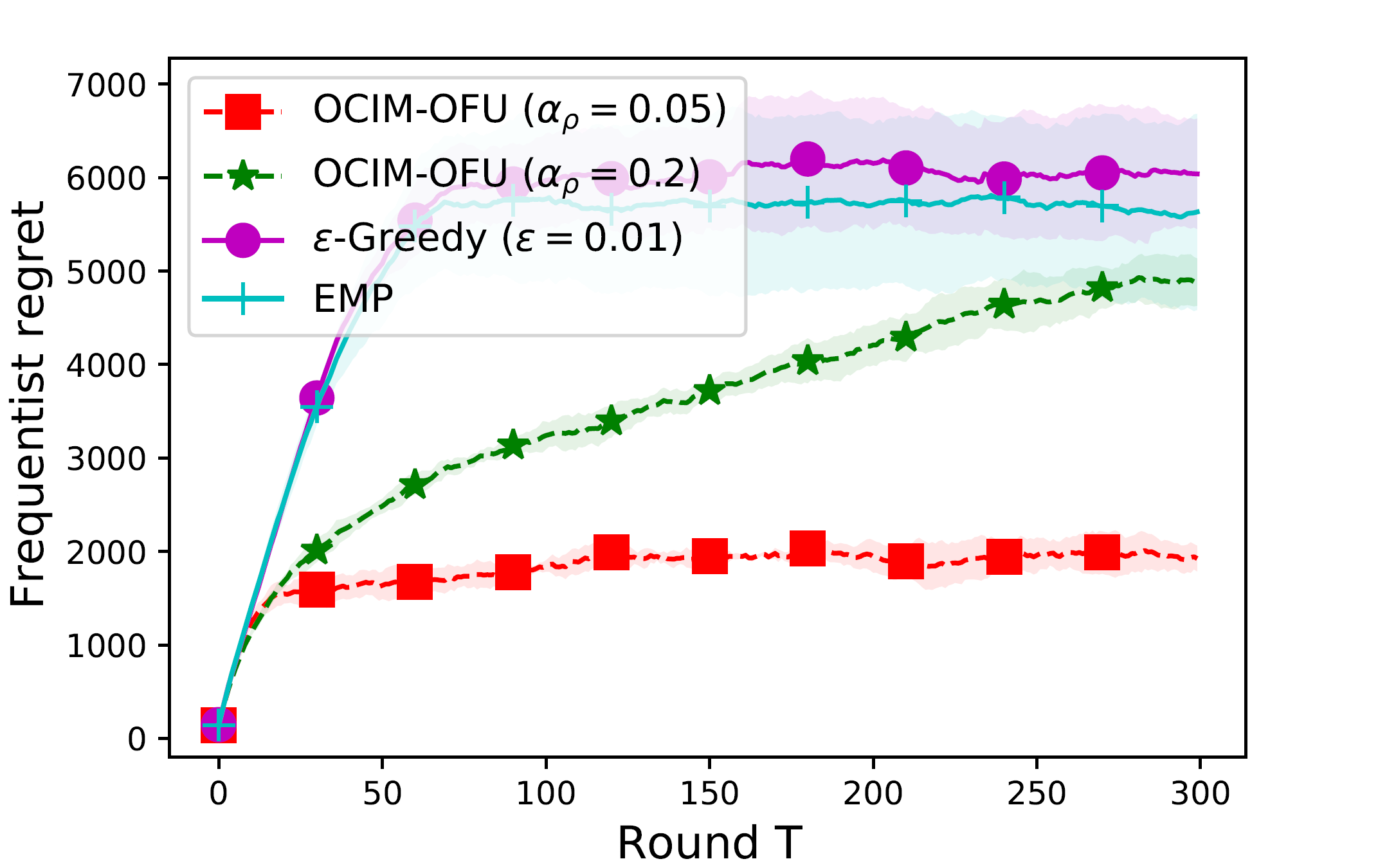
Experimental result for frequentist regrets Figures 2(a) and 2(b) show the results for Yahoo-Ad. First, the regret of OCIM-OFU grows sub-linearly with respect to round for all , consistent with Theorem 5.1’s regret bound. Second, we can observe that OCIM-OFU is superior to EMP and -Greedy when . When , OCIM-OFU may have larger regret due to too much exploration. The OCIM-TS algorithm has larger slope in regrets compared to other algorithms. We speculate that such large slope comes from the uninformative prior, which requires more rounds to compensate for the mismatch of the uninformative and the true priors.
The results on the DM dataset are shown in Figs. 2(c) and 2(d). Generally, they are consistent with those on the Yahoo-Ad dataset: OCIM-OFU also grows sub-linearly w.r.t round . When , OCIM-OFU has smaller regret than all baselines. Moreover, the difference between OCIM-OFU and the baselines for the non-strategic competitor (RD) is more significant than that of the strategic competitor’s (IM), because the non-strategic competitor is less “dominant” and OCIM-OFU can carefully trade off exploration and exploitation to maximize ’s influence. OCIM-TS learns faster and achieves better performance in this dataset compared to that in the Yahoo-Ad dataset.


Experimental result for Bayesian regrets We show Bayesian regrets of all algorithms in Figure 3. All algorithms except for OCIM-TS have similar curves. OCIM-TS, however, achieves at least two orders of magnitudes lower regret () compared with other algorithms. The reason is that OCIM-TS leverages its prior knowledge to quickly converge to the optimal solution, but other algorithms cannot use this knowledge effectively.
8 Conclusion and Future Work
In this paper, we formulate the OCIM problem and introduce a general C2MAB-T framework for it. We prove that one important condition required by prior CMAB algorithms, the TPM condition, still holds, while the other one, monotonicity, is not satisfied. We propose three algorithms that balance between prior knowledge, offline computation, feedback and regret bound: OCIM-TS relies on prior knowledge and achieves logarithmic Bayesian regret; OCIM-OFU needs to solve a harder offline problem and achieves logarithmic frequentist regret; and OCIM-ETC requires less feedback at the expense of a worse frequentist regret bound. We extend our framework to settings with more complex competitor actions.
This paper initiates the first study on OCIM, and it opens up a number of future directions. One is to design efficient offline approximation algorithms in the competitive setting when edge probabilities take a range of values. Another interesting direction is to study other partial feedback models, e.g. we only observe feedback from edges triggered by but not . A further direction is to look into distributed online learning, when competitors and both learn from the propagation and deploy their seeds accordingly.
Acknowledgements
John C.S. Lui is supported in part by the GRF 14200321.
References
- Bharathi et al., (2007) Bharathi, S., Kempe, D., and Salek, M. (2007). Competitive influence maximization in social networks. In International workshop on web and internet economics, pages 306–311.
- Borgs et al., (2014) Borgs, C., Brautbar, M., Chayes, J., and Lucier, B. (2014). Maximizing social influence in nearly optimal time. In Proceedings of the twenty-fifth annual ACM-SIAM symposium on Discrete algorithms, pages 946–957.
- Budak et al., (2011) Budak, C., Agrawal, D., and El Abbadi, A. (2011). Limiting the spread of misinformation in social networks. In Proceedings of the 20th international conference on World wide web, pages 665–674.
- Carnes et al., (2007) Carnes, T., Nagarajan, C., Wild, S. M., and Van Zuylen, A. (2007). Maximizing influence in a competitive social network: a follower’s perspective. In Proceedings of the ninth international conference on Electronic commerce, pages 351–360.
- Chen et al., (2018) Chen, L., Xu, J., and Lu, Z. (2018). Contextual combinatorial multi-armed bandits with volatile arms and submodular reward. Advances in Neural Information Processing Systems, 31:3247–3256.
- Chen et al., (2011) Chen, W., Collins, A., Cummings, R., Ke, T., Liu, Z., Rincon, D., Sun, X., Wang, Y., Wei, W., and Yuan, Y. (2011). Influence maximization in social networks when negative opinions may emerge and propagate. In Proceedings of the 2011 siam international conference on data mining, pages 379–390. SIAM.
- Chen et al., (2013) Chen, W., Lakshmanan, L. V. S., and Castillo, C. (2013). Information and Influence Propagation in Social Networks. Morgan & Claypool Publishers.
- Chen et al., (2016) Chen, W., Wang, Y., Yuan, Y., and Wang, Q. (2016). Combinatorial multi-armed bandit and its extension to probabilistically triggered arms. The Journal of Machine Learning Research, 17(1):1746–1778.
- Garivier et al., (2016) Garivier, A., Lattimore, T., and Kaufmann, E. (2016). On explore-then-commit strategies. In Advances in Neural Information Processing Systems, pages 784–792.
- He et al., (2012) He, X., Song, G., Chen, W., and Jiang, Q. (2012). Influence blocking maximization in social networks under the competitive linear threshold model. In Proceedings of the 2012 siam international conference on data mining, pages 463–474.
- Hüyük and Tekin, (2020) Hüyük, A. and Tekin, C. (2020). Thompson sampling for combinatorial network optimization in unknown environments. IEEE/ACM Transactions on Networking, 28(6):2836–2849.
- Ivanov et al., (2017) Ivanov, S., Theocharidis, K., Terrovitis, M., and Karras, P. (2017). Content recommendation for viral social influence. In Proceedings of the 40th International ACM SIGIR Conference on Research and Development in Information Retrieval, pages 565–574.
- Kempe et al., (2003) Kempe, D., Kleinberg, J., and Tardos, É. (2003). Maximizing the spread of influence through a social network. In Proceedings of the ninth ACM SIGKDD international conference on Knowledge discovery and data mining, pages 137–146.
- Li et al., (2020) Li, S., Kong, F., Tang, K., Li, Q., and Chen, W. (2020). Online influence maximization under linear threshold model. In Advances in Neural Information Processing Systems.
- Li et al., (2018) Li, Y., Fan, J., Wang, Y., and Tan, K. (2018). Influence maximization on social graphs: A survey. IEEE Trans. Knowl. Data Eng., 30(10):1852–1872.
- Lin and Lui, (2015) Lin, Y. and Lui, J. C. (2015). Analyzing competitive influence maximization problems with partial information: An approximation algorithmic framework. Performance Evaluation, 91:187–204.
- Liu et al., (2021) Liu, X., Zuo, J., Chen, X., Chen, W., and Lui, J. C. (2021). Multi-layered network exploration via random walks: From offline optimization to online learning. In International Conference on Machine Learning, pages 7057–7066. PMLR.
- Merlis and Mannor, (2020) Merlis, N. and Mannor, S. (2020). Tight lower bounds for combinatorial multi-armed bandits. Proceedings of Thirty Third Conference on Learning Theory.
- Nguyen et al., (2016) Nguyen, H. T., Thai, M. T., and Dinh, T. N. (2016). Stop-and-stare: Optimal sampling algorithms for viral marketing in billion-scale networks. In SIGMOD, pages 695–710.
- Perrault et al., (2020) Perrault, P., Healey, J., Wen, Z., and Valko, M. (2020). Budgeted online influence maximization. In International Conference on Machine Learning, pages 7620–7631. PMLR.
- Qin et al., (2014) Qin, L., Chen, S., and Zhu, X. (2014). Contextual combinatorial bandit and its application on diversified online recommendation. In Proceedings of the 2014 SIAM International Conference on Data Mining, pages 461–469. SIAM.
- Russo and Van Roy, (2014) Russo, D. and Van Roy, B. (2014). Learning to optimize via posterior sampling. Mathematics of Operations Research, 39(4):1221–1243.
- Russo and Van Roy, (2016) Russo, D. and Van Roy, B. (2016). An information-theoretic analysis of thompson sampling. The Journal of Machine Learning Research, 17(1):2442–2471.
- Tang et al., (2009) Tang, J., Sun, J., Wang, C., and Yang, Z. (2009). Social influence analysis in large-scale networks. In Proceedings of the 15th ACM SIGKDD international conference on Knowledge discovery and data mining, pages 807–816.
- Tang et al., (2018) Tang, J., Tang, X., Xiao, X., and Yuan, J. (2018). Online processing algorithms for influence maximization. In SIGMOD, pages 991–1005.
- Tang et al., (2015) Tang, Y., Shi, Y., and Xiao, X. (2015). Influence maximization in near-linear time: A martingale approach. In Proceedings of the 2015 ACM SIGMOD International Conference on Management of Data, pages 1539–1554.
- Vaswani et al., (2017) Vaswani, S., Kveton, B., Wen, Z., Ghavamzadeh, M., Lakshmanan, L. V., and Schmidt, M. (2017). Model-independent online learning for influence maximization. In Proceedings of the 34th International Conference on Machine Learning, pages 3530–3539.
- Wang and Chen, (2017) Wang, Q. and Chen, W. (2017). Improving regret bounds for combinatorial semi-bandits with probabilistically triggered arms and its applications. In Advances in Neural Information Processing Systems, pages 1161–1171.
- Wang and Chen, (2018) Wang, S. and Chen, W. (2018). Thompson sampling for combinatorial semi-bandits. In International Conference on Machine Learning, pages 5114–5122. PMLR.
- Wen et al., (2017) Wen, Z., Kveton, B., Valko, M., and Vaswani, S. (2017). Online influence maximization under independent cascade model with semi-bandit feedback. In Advances in neural information processing systems, pages 3022–3032.
- Wu et al., (2019) Wu, Q., Li, Z., Wang, H., Chen, W., and Wang, H. (2019). Factorization bandits for online influence maximization. In Proceedings of the 25th ACM SIGKDD International Conference on Knowledge Discovery & Data Mining, pages 636–646.
Appendix
Appendix A Proof of Theorem 3.1
Proof.
Let be the probability that node is activated by . From the proof of Lemma 2 in (Wang and Chen, 2017), we know that if for every node and every and vectors we have
| (6) |
then Theorem 3.1 is true. Notice that
| (7) | ||||
| (8) |
where and are two live-edge graphs sampled under and , respectively. As mentioned in Sec. 3.2, we use an edge coupling method to compute the difference between and . Specifically, for each edge , suppose we independently draw a uniform random variable over , let
where represents the live/blocked state of edge in live-edge graph . Notice that and does not have the subgraph relationship. Let , the difference can be written as:
| (9) |
where . Since could be 0, 1 or -1, we will discuss these cases separately.
1) .
This will not contribute to the expectation.
2) .
This will occur only if there exists a path such that: under , can be activated by via this path, while under , cannot be activated by via this path. We denote this event as . We will show that occurs only if at least one of and occurs.
: There exists a path such that:
1. is activated by under both and
2. edge is live under but not
: There exists a path such that:
1. is activated by under both and
2. edge is live under but not
Lemma A.1.
occurs only if at least one of and occurs.
Proof.
Let us first discuss the relationship between , and . For , if can be activated by under but not , it is because either: (a) some edge is live in but blocked in while is -activated (or equivalently is -triggered); or (b) some edge is live in but blocked in while is -triggered. The former could be relaxed to , and the latter could be relaxed to . Notice that and are not mutually exclusive and we are interested in the upper bound of .

Assuming is true, consider the shortest path from one seed node of , , to node , such that under node is activated by but under it is not. When is true, there must exist a node that is not activated by in under . We denote the first node from to (i.e., closest to ) in that is not activated by under as .
Next, let us consider the live/blocked state of edge . We already know edge is live under . If edge is blocked under , since is activated by under both and , it directly becomes . Otherwise, if edge is live under , the reason that node is not activated by could only be that it is activated by . In this case, there must exist a path from one seed node of , , to node , such that is activated by under but not . This can only occur when there exists a node that is not activated by in under . We denote the first node from to (i.e., closest to ) in that is not activated by under as . Notice that when the tie-breaking rule is , we have as should arrive at earlier than ; when the tie-breaking rule is , we have as should arrive at no later than . We will discuss the case of the proportional tie-breaking rule separately after the discussion of the dominance tie-breaking rules.
Then, let us consider the live/blocked state of edge . We already know edge is live under . If edge is blocked under , since is activated by under both and , it directly becomes . Otherwise, if edge is live under , the reason that node is not activated by could only be that it is activated by . It also means neither nor occurs so far. In this case, there must exist a path from one seed node of , , to node , such that is activated by under but not . This can only occur when there exists a node that is not activated by in under . We denote the first node from to (i.e., closest to ) in that is not activated by under as . Notice that when , we have as should arrive at no later than ; when , we have as should arrive at earlier than .
Now let us consider the live/blocked state of edge . We already know edge is live under . If edge is blocked under , since is activated by under both and , it directly becomes . Otherwise, if edge is live under , the reason that node is not activated by could only be that it is activated by . In this case, there must exist a path from one seed node of , , to node , such that is activated by under but not . This can only occur when there exists a node that is not activated by in under . We denote the first node from to (i.e., closest to ) in that is not activated by under as . Notice that when , we have as should arrive at earlier than ; when , we have as should arrive at no later than .
Again, let us consider the live/blocked state of edge . We already know edge is live under . If edge is blocked under , since is activated by under both and , it directly becomes . Otherwise, if edge is live under , similar to the discussion above, we need to consider a new path with length and .
For the case of the proportional tie-breaking rule, in addition to the edge coupling, we also need to couple the permutation order (Chen et al., 2011) for each node in and . More specific, for each node , we randomly permute all of its in-neighbors, then when we need to break a tie on , we find its activated neighbor that is ordered first in the permutation order, and assign the state of as ’s state. Assuming the same permutation order in and , let us consider path and again. If , then must be . If does not occur in , then the only neighbor of in must be ordered before the only neighbor of in in the permutation order on . However, if does not occur in , with such permutation order, it is impossible that is activated by under but not . As a result, if neither nor occurs in path and , we have in the case of the proportional tie-breaking rule.
To sum up, if neither nor occurs in path and , we need to check whether they could occur in a new path shorter than , and shorter than . As a result, we only need to check whether or occurs in the path with only one edge. In that case, or occurs for sure. Thus, by induction, we conclude that at least one of and occurs when considering any path with more than one edge, so will occur only if at least one of and occurs. ∎
Now, let us consider the two events in for a specific edge . We find that the first event { is activated by under both and }, is independent of the second event {edge is live under but not }, since the live/blocked state of edge does not affect the activation of its tail node . Also, for edge , the probability of these two events can be written as
| (10) | ||||
| (11) |
As a result, we have:
| (12) |
Since and are symmetric, we also have:
| (13) |
Combining with Lemma. A.1, we have
| (14) |
3) .
Similar to the previous case, this will occur only if there exists a path such that: under , can be activated by via this path, while under , cannot be activated by via this path. We denote this event as . We show that occurs only if at least one of and occurs.
: There exists a path such that:
1. is activated by under both and
2. edge is live under but not
: There exists a path such that:
1. is activated by under both and
2. edge is live under but not
Since they are symmetric with and , following the same analysis, we can get
| (15) | ||||
| (16) | ||||
| (17) |
Combining all cases together, we have:
| (18) |
The last inequality above is due to:
Notice that Eq.(18) could be relaxed to:
| (19) |
∎
Appendix B Proof of Theorem 4.1
Proof.
We define as the feedback of OCIM in round , which includes the outcomes of for all . We denote by the history of observations available to the player when choosing an action . For the Bayesian analysis, we assume the mean vector follows a prior distribution . In round , given , we define the posterior distribution of as (i.e., where is given in Alg. 1). As mentioned in Section 4, OCIM-TS allows any benchmark offline oracles, including approximation oracles. We consider a general benchmark oracle . As oracle might be a randomized policy (e.g., an -approximation oracle with success probability ), we use a random variable to represent all its randomness. In order to discuss the performance of OCIM-TS with oracle , we rewrite the Bayesian regret in Eq.(2) as
| (20) |
Notice that is the action taken by the player if the true is known, while is the real action chosen by OCIM-TS. The original regret definition in Eq.(2) is a special case of Eq.(20) for an -approximation oracle, and will focus on this general form in this proof.
The key step to derive the Bayesian regret bound of OCIM-TS is to show that the conditional distributions of and given are the same:
| (21) |
which is true since we use Thompson sampling to update the posterior distribution of . With this finding, we consider the Bayesian regret in Eq.(2):
| (22) | ||||
| (23) | ||||
| (24) | ||||
| (25) |
where Eq.(24) comes from applying Eq.(21) to Eq.(23). Let and , where and is the total number of times arm is played until round . We define and . By Eq.(25), we have
| (26) | ||||
| (27) |
We can bound these three terms separately. For term (a), when , we could bound . When and (Definition 7 in (Wang and Chen, 2017)) holds, by the proof of Lemma 5 in (Wang and Chen, 2017), we have where is the set of arms triggered by and is defined in (Wang and Chen, 2017). We have
For term (b), we can observe that , since is determined given , and given , and follow the same distribution. Since , we have
For term (c), we can bound it by
For term (d), similar to Eq.(20) in (Wang and Chen, 2017), we have
Combine them together, we have
where . Take , we finally get finally get the Bayesian regret bound of TS-OCIM:
∎
Appendix C Proof of Theorem 5.1
Proof.
We first introduce the following definitions to assist our analysis. Recall that is the action space in round . We define the reward gap for all actions . For each base arm , we define and . If there is no action such that and , we define and . We define and . Let be the set of arms that can be triggered by . We define as the largest number of arms could be triggered by a feasible action. We use to denote . If , we provide the distribution-dependent bound of the OCIM-OFU algorithm.
To prove the distribution-dependent and the distribution-independent regret bounds, we generally follow the proof of Theorem 1 in Wang and Chen, 2017. However, since we extend the original CMAB problem to a new contextual setting where the action space is the context, and monotonicity does not hold in the OCIM setting, we need to modify their analysis to tackle these changes. We introduce a positive real number for each arm and define . Define
where
Let be the event that at the beginning of round , for every arm , . Let be the event that at round oracle outputs a solution, and , such that , i.e., oracle fails to output an -approximate solution. Let be the event that the triggering is nice at the beginning of round (Definition 7 in (Wang and Chen, 2017)). The following lemma explains how contributes to the regret.
Lemma C.1.
For any vector of positive real numbers and , if and hold, we have
where is the index of the TP group with (see Definition 5 in (Wang and Chen, 2017)).
Proof.
By and for all , we have
| (28) |
It means that we have the correct estimated range of for all at round . Combining with for the offline oracle , we have
| (29) |
By the TPM condition in Theorem. 3.1, we have
| (30) |
We want to bound by bounding . We first perform a transformation. Since , we have . Then we have
| (31) |
In fact, if holds and for all ,
| (32) |
So far, all requirements on bounding in Lemma 5 from (Wang and Chen, 2017) are also satisfied by of OCIM-OFU algorithm in the OCIM setting without monotonicity. We can then follow the same steps to bound in the two cases they considered (combining their Eq.(11)-(13)) and get
∎
With Lemma C.1, we can follow the proof of Lemma 6 in (Wang and Chen, 2017) to bound the regret when and hold.
| (33) |
Finally, we take . If , then , since we have either or for some . Thus, no regret is accumulated when . Following Eq.(17)-(21) in (Wang and Chen, 2017), we can derive the distribution-dependent regret bound
| (34) |
To derive the distribution-independent bound, we take , follow Eq.(23) in (Wang and Chen, 2017) and get
| (35) |
∎
Appendix D Computational Efficiency of OCIM-OFU
D.1 Proof of Theorem 5.2
Proof.
In order to prove Theorem 5.2, we first introduce a new optimization problem denoted as : given , the new problem aims to find the optimal for one edge to maximize , while fixing the values of all others. The following lemma shows it is #P-hard.
Lemma D.1.
Given and fixing for all , finding the optimal for one edge that maximizes is #P-hard.
Proof.
We prove the hardness of this optimization problem via a reduction from the influence computation problem. We first consider a general graph with nodes and edges, where all influence probabilities on edges are set to . Given , computing the influence spread of in such a graph is #P-hard. Notice that there is no seed set of in . Now let us take one node in and denote its activation probability by as . Actually, computing is also #P-hard and we want to show that it can be reduced to our optimization problem in polynomial time.

We first construct a new graph based on . For , we keep and unchanged, then add several nodes and edges as shown in Fig. 5. We add node to the seed set of and node to the seed set of , so the joint action . In this new graph , we consider the optimization problem of finding the optimal (influence probability on edge ) within its range that maximizes . Notice that the influence probability on edge is a constant and would only affect the activation probability of node . We denote the activation probability by of node as . In order to maximize , we only need to maximize . It can be written as:
| (36) |
It is easy to see has a linear relationship with , so the optimal could only be either the lower or upper bound of its range . Assuming we can solve the optimization problem of finding the optimal , then we can determine the sign of ’s coefficient in Eq.(36): if the optimal is the upper bound value in , we have ; otherwise, . It means we can answer the question that whether is larger (or smaller) than . Notice that , so we can manually change the value of to check whether is larger (or smaller) than for any , Recall that all edge probabilities in are set to , so the highest precision of should be . Hence, we can use a binary search algorithm to find the exact value of in at most times. It means computing the activation probability of in can be reduced to the optimization problem of finding the optimal in , which completes the proof. ∎
We then show that is a special case of Eq.(4). The main idea is to relax the constraints in Eq.(4) and show that it can find the optimal for any given . Consider a graph with nodes and a given seed set . We construct a new graph by manually add additional nodes pointing from each seed node in . If we can solve the optimization problem Eq.(4) in the new graph , since must be the optimal seed set of and the added nodes will not affect the prorogation in , we will also find the optimal ’s in the original graph for the given . Then, it is easy to see is a special case of Eq.(4) since only find the optimal for one edge . With Lemma D.1, we know Eq.(4) is also #P-hard.
∎
D.2 Non-submodularity of
In Section 5.1, we introduce , which is an upper bound function of for each . If is submodular over , we can use a greedy algorithm on to find an approximate solution. However, the following example in Fig. 6 shows that is not submodular.

In Fig. 6, the numbers attached to edges are influence probabilities. Only the influence probability of edge is a variable and we denote it as . We assume and . Let us consider some choices of . When is chosen as or , the optimal that maximizes is 1; when is chosen as , the optimal that maximizes is 0. Based on this observation, we can calculate (assuming ):
Thus we have
| (37) |
which is contrary to submodularity.
D.3 Bipartite Graph
We consider a weighted bipartite graph where each edge is associated with a probability . Given the competitor’s seed set , we need to choose nodes from as that maximizes the expected number of nodes activated by in , where a node can be activated by a node with an independent probability of . As mentioned before, if and are attempting to activate a node in at the same time, the result will depend on the tie-breaking rule. If all edge probabilities are fixed, i.e., is fixed, is still submodular over , so we can use a greedy algorithm as a -approximation oracle . Based on it, let us discuss the new offline optimization problem in Eq.(4) under our two tie-breaking rules: (1) : since will never influence nodes in earlier than in bipartite graphs, and will always win the competition, from ’s perspective, we can ignore to choose . In this case, all edge probabilities should take the maximum values: for all , equals to the upper bound of , and we then use the oracle to find . (2) : since will never influence nodes in earlier than in bipartite graphs, and will always win the competition, all out-edges of , denoted as , should take the minimum probabilities to maximize the influence spread of . All the other edges in should take the maximum probabilities. Formally, for all , equals to the lower bound of ; for all , equals to the upper bound of . We then use the oracle to find . To sum up, in bipartite graphs, is optimized by pre-determining based on the tie-breaking rule, and then using the greedy algorithm to get a -approximation solution. Since the time complexity of influence computation in the bipartite graph is , the time complexity of the offline algorithm is equal to that of the greedy algorithm, .
D.4 General Graph
GraphWe The competitive propagation in the general graph is much more complicated, so it is hard to pre-determine all edge probabilities as in the bipartite graph case. However, we have a key observation:
Lemma D.2.
When fixing the seed set , reward has a linear relationship with each (when other ’s with are fixed). This implies that the optimal solution for the optimization problem in Eq.(4) must occur at the boundaries of the intervals ’s.
Proof.
We can expand based on the live-edge graph model (Chen et al., 2013a):
| (38) |
where is one possible live-edge graph (each edge is in with probability and not in with probability , and this is independent from other edges), is the set of nodes activated by from seed sets under live-edge graph and is the set of edges that appear in live-edge graph . Eq.(38) shows that is linear with each , so the optimal must take either the minimum or the maximum value in its range . ∎
Lemma D.2 implies that for any edge not reachable from seeds, it is safe to always take its upper bound value since it can only helps the propagation of . This further suggests that if we only have a small number (e.g. ) of edges reachable from , then we can afford enumerating all the boundary value combinations of these edges. For each such boundary setting , we can use the IMM algorithm (Tang et al., 2014) to design a -approximation oracle with time complexity . We discuss such graphs that satisfy the above condition in directed trees. Specifically, we consider the in-arborescence, where all edges point towards the root. For any node in the in-arborescence, there only exists one path from to the root; if is selected as the seed node of , it could only propagate via this path. Hence, if the depth of the in-arborescence is in the order of , the number of edges reachable from would be . In this case, we can use the IMM algorithm for combinations to obtain an approximate solution with time complexity . Examples of such in-arborescences with depth could be the complete or full binary trees.
For general graphs, designing efficient approximation algorithms for the offline problem in Eq. (4) remains a challenging open problem, due to the joint optimization over and and the complicated function form of . Nevertheless, heuristic algorithms are still possible. In the experiment section, we employee the following heuristic with the tie-breaking rule: for all outgoing edges from seeds, we set their influence probabilities to their lower bound values, while for the rest, we set them to their upper bound values. This setting guarantees that the first-level edges from the seeds are always set correctly, no matter how we select seeds. They do not guarantee the correctness of second or higher level edge settings in the cascade, but the impact of those edges to influence spread decays significantly, so the above choice is reasonable as a heuristic.
Appendix E Proof of Theorem 5.3
Proof.
The OCIM-ETC algorithm is described in Alg. 3. We utilize the following well-known tail bound in our proof.
Lemma E.1.
(Hoeffding’s Inequality) Let be independent and identically distributed random variables with common support and mean . Let . Then for all ,
Let be the empirical mean of . Recall that oracle takes and as inputs and outputs a solution . Let us define event , which represents that oracle fails to output an -approximate solution, and we know .
With the same definitions in Appendix C, we can decompose the regret as:
| (39) |
Next, let us rewrite the TPM condition in Theorem 3.1. For any , and , we have
| (40) |
where is the maximum number of nodes that any one node can reach in graph . Let denote the optimal action for in round . Under , we have
| (41) |
where the third inequality is due to Eq.(40). Combining Eq.(40) and Eq.(41) together, we have
| (42) |
Let us define . If , then we know is at least an -approximate solution, such that . Then the regret in Eq.(39) can be written as
| (43) |
The first inequality is obtained by applying the Hoeffding’s Inequality (Lemma E.1) and union bound to the event . Now we need to choose an optimal that minimizes Eq.(43). By taking , when , we can get the distribution-dependent bound
| (44) |
Next, let us prove the distribution-independent bound. Let denote the event that for all . By the Hoeffding’s Inequality and union bound, we have
| (45) |
When holds, with Eq.(42), we have
| (46) |
and the regret in Eq.(39) can be written as
| (47) |
We can choose so as to (approximately) minimize the regret. For , we obtain:
| (48) |
To complete the proof, we need to consider both and . As shown in Eq.(45), the probability that occurs is very small, and we have:
| (49) |
∎
Appendix F Proof of Theorem 6.1
Proof.
As mentioned in Section 6, we need to introduce a virtual seed node , which connects to each existing node with an unknown edge probability equal to the probability of being selected as a seed. By adding these virtual nodes and edges, we get a new graph with nodes and edges. Since is fixed under , we can follow the same steps in the proof of Theorem 3.1 to show the TPM condition holds under . Note that the maximum number of nodes that any one node can reach in is twice as that in the original graph , so the new bounded smoothness coefficient . ∎
Appendix G Additional Experiments
G.1 Experiments for Tie-breaking Rule
When we consider in bipartite graphs, we can trivially ignore to choose since the influence spread ends in one diffusion round, and OCIM becomes the online influence maximization problem without competition. We show such results in Figure 7. Note that the distribution of no longer affects the performance of when and we only use one figure for the IM and RD distribution. For general graphs, we use the same DM dataset and parameter settings described in Sec. 7, and the only difference is that now dominates . We show the results in Figure 8. Overall, the results and the analysis for are consistent with .
G.2 Experiments for OCIM-ETC
We show the frequentist/Bayesian regret results for the OCIM-ETC algorithm in Figure 9, Figure 10 and Figure 11. In Figure 9, we set exploration phase to be rounds and the experiments show that we suffer linear regrets in both the exploration and the exploitation phase, meaning that the unknown parameters are under-explored. Thus we reset exploration to be and Figure 11 shows that OCIM-ETC now has constant regret in the exploitation phase. For DM dataset, since the node number and the edge number are less than Yahoo-Ad, we can see constant regrets after rounds of exploration in Figure 10. Compared with OCIM-OFU/OCIM-TS, OCIM-ETC requires more rounds to learn the unknown influence probabilities and has larger regrets than OCIM-OFU/OCIM-TS, but with sufficient exploration (which is much less than the theoretical requirements in Theorem 5.3) OCIM-ETC can yield constant regrets during the exploitation phase in our experiments.


G.3 Experiments for Probabilistic Seed Distribution
For the settings where the competitor has unknown fixed seed distribution, we first run the non-competitive influence maximization algorithm for . and get the best seeds on Yahoo-Ad and the best seeds on DM, respectively, We then consider the seed distribution of as choosing each node from the best seeds with probability , i.e., the probability that choosing all best seeds on Yahoo-Ad is and the probability that choosing all best seeds on DM is . This seed distribution of is unknown to our algorithms. In our experiments, we set for Yahoo-Ad and for DM, and assume . Figure 12 shows that OCIM-OFU is still superior to EMP and -Greedy for this setting with more complex competitor actions. We omit the results of OCIM-TS here as it requires the prior knowledge of the competitor’s seed distribution. However, as long as the given prior does not differ much from the true prior, OCIM-TS will also achieve good regret results.

Appendix H Contextual combinatorial multi-armed bandit framework C2MAB-T
H.1 General Framework
We propose a general framework of contextual combinatorial multi-armed bandit with probabilistically triggered arms (C2MAB-T), which is a contextual extension of CMAB-T in (Wang and Chen, 2017).
C2MAB-T is a learning game between a learning player and an environment. The environment consists of random variables called base arms following a joint distribution over . Distribution is chosen by the environment from a class of distributions before the game starts. The player knows but not the actual distribution in advance. Different from that in CMAB-T, the environment in C2MAB-T also provides contexts for the learning agent, which will be discussed in detail later.
The learning process runs in discrete rounds. In round , the environment first provides a context, , to the player, where is the full action space and is a subset of it, representing the current action space in round . The player then chooses an action based on the feedback history from previous rounds. The environment also draws an independent sample from the joint distribution . When action is played on the environment outcome , a random subset of arms are triggered, and the outcomes of for all are observed as the feedback to the player. may have additional randomness beyond the randomness of . Let denote a distribution of the triggered subset of for a given action and an environment outcome . We assume is drawn independently from . The player obtains a reward fully determined by and . A learning algorithm aims at selecting actions ’s over time based on the past feedback to accumulate as much reward as possible.
For each arm , let . Let denote the expectation vector of arms. We assume that the expected reward , where the expectation is taken over and , is a function of action and the expectation vector of the arms. Thus, we denote . We assume the outcomes of arms do not depend on whether they are triggered, i.e., .
The performance of a learning algorithm is measured by its expected regret, which is the difference in expected cumulative reward between always playing the best action and playing actions selected by algorithm . Let denote the expected reward of the optimal action in round . We assume that there exists an offline oracle , which takes context and as inputs and outputs an action such that , where is the approximation ratio and is the success probability. Instead of comparing with the exact optimal reward, we take the fraction of it and use the following -approximation frequentist regret for rounds:
| (50) |
where is the action chosen by algorithm in round .
Another way to measure the performance of the algorithm is using Bayesian regret. Denote the prior distribution of as . When the prior is given, the corresponding Bayesian regret is defined as:
| (51) |
Note that the contextual combinatorial bandit problem is also studied in (Chen et al., 2018; Qin et al., 2014). They consider the context features of all bases arms, which can affect their expected outcomes in each round, and assume the action space of super arms is a subset of . However, we do not bond the context with base arms and consider the feasible set of super arms, , as the context, which is more flexible than a subset of . Besides, we are the first to consider probabilistically triggered arms in the contextual combinatorial bandit problem.
H.2 Monotonicity and Triggering Probability Modulated Condition
In order to guarantee the theoretical regret bounds, we consider two conditions given in (Wang and Chen, 2017). The first one is monotonicity, which is stated below.
Condition 3.
(Monotonicity). We say that a C2MAB-T problem instance satisfies monotonicity, if for any action , for any two expectation vectors and , we have if for all .
The second condition is Triggering Probability Modulated (TPM) Bounded Smoothness. We use to denote the probability that the action triggers arm when the expectation vector is . The TPM condition in C2MAB-T is given below.
Condition 4.
(1-Norm TPM bounded smoothness). We say that a C2MAB-T problem instance satisfies 1-norm TPM bounded smoothness, if there exists (referred as the bounded smoothness coefficient) such that, for any two expectation vectors and , and any action , we have .
H.3 Regret Bounds with Monotonicity
For the general C2MAB-T problem that satisfies both monotonicity (Condition 3) and TPM bounded smoothness (Condition 4), we introduce a contextual version of the CUCB algorithm (Wang and Chen, 2017), which is described in Algorithm 4. Recall that is the action space in round . We define the reward gap for all actions . For each arm , we define and . If there is no action such that and , we define and . We define and . Let be the set of arms that can be triggered by . We define as the largest number of arms could be triggered by a feasible action. We use to denote . Contextual CUCB (C2-UCB) has the following regret bounds.
Theorem H.1.
Proof.
We first show that Lemma 5 in (Wang and Chen, 2017) still holds for Contextual CUCB algorithm in the C2MAB-T problem. Let be the event that at the beginning of round , for every arm , . Let be the event that at round oracle fails to output an -approximate solution. In Lemma 5 from (Wang and Chen, 2017), it assumes that and hold, then we have
| (53) |
By the TPM condition, we have
| (54) |
which is in the same form of Eq.(10) in (Wang and Chen, 2017). Hence, we can follow the remaining proof of its Lemma 5. With Lemma 5, we can follow the proof of Lemma 6 in (Wang and Chen, 2017) to bound the regret when , where and is a positive real number for each arm . Finally, we take . If , then , since we have either or for some . Thus, no regret is accumulated when . Following Eq.(17)-(22) in (Wang and Chen, 2017), we can derive the distribution-dependent and distribution-independent regret bounds shown in the theorem. ∎
H.4 Regret Bounds without Monotonicity
As discussed in Section 3, OCIM is an example of C2MAB-T that satisfies the TPM condition but not monotonicity. For the general C2MAB-T problem without monotonicity, we proposed two algorithms, C2-TS, C2-OFU, that can still achieve logarithmic Bayesian and frequentist regrets respectively. We also present C2-ETC that has a tradeoff between feedback requirement and regret bound.
C2-TS is described in Algorithm 5. Different from OCIM-TS, we input a general prior (which depends on and might not be Beta distributions anymore) and update the posterior distribution accordingly. With the same definitions in H.3 and , it has the following Bayesian regret bound.
Theorem H.2.
C2-OFU is described in Algorithm 6. Similar to OCIM-OFU, it requires an offline oracle that takes the context and ’s (ranges of ’s) as inputs and outputs an approximate solution . With such an oracle, C2-OFU has the following frequentist regret bounds.
Theorem H.3.
Besides C2-TS and C2-OFU, we also provide a general explore-then-commit algorithm C2-ETC, as described in Algorithm 7. In the general setting, is defined as the set of base arms that is deterministically triggered by the action in question. C2-ETC is simple and only requires feedback from directly triggered arms, but it has a worse regret bound and requires the following condition besides Condition 4.
Condition 5.
For some , given any context and any set with , there exists such that for every .
With such a condition, C2-ETC has the following frequentist regret bounds.