跳到论文正文
W Papers独立论文阅读器 arXiv:2006.13330 论文正文 计算阅读时间 · 0%
引用这篇论文根据当前论文元数据生成,正式投稿前建议核对。


License: arXiv.org perpetual non-exclusive license
arXiv:2006.13330v2 [math.ST] 03 Jul 2020
††footnotetext: †Department of Management Science, Stanford University, CA 94043, USA.
∗Department of Electrical Engineering, Stanford University, CA 94043, USA.
‡Department of Radiation Oncology, Stanford University, CA 94043, USA.

A Mean-Field Theory for Learning the Schönberg Measure of Radial Basis Functions

Masoud Badiei Khuzani†,‡, Yinyu Ye†, Sandy Napel‡,∗, Lei Xing‡,∗ Address: Stanford University, 450 Serra Mall, Stanford, CA 94305 Current address: Email address: mbadieik,yyye,snapel,lei@stanford.edu
Abstract.

We develop and analyze a projected particle Langevin optimization method to learn the distribution in the Schönberg integral representation of the radial basis functions from training samples. More specifically, we characterize a distributionally robust optimization method with respect to the Wasserstein distance to optimize the distribution in the Schönberg integral representation. To provide theoretical performance guarantees, we analyze the scaling limits of a projected particle online (stochastic) optimization method in the mean-field regime. In particular, we prove that in the scaling limits, the empirical measure of the Langevin particles converges to the law of a reflected Itô diffusion-drift process. The distinguishing feature of the derived process is that its drift component is also a function of the law of the underlying process. Using Itô lemma for semi-martingales and Grisanov’s change of measure for the Wiener processes, we then derive a Mckean-Vlasov type partial differential equation (PDE) with Robin boundary conditions that describes the evolution of the empirical measure of the projected Langevin particles in the mean-field regime. In addition, we establish the existence and uniqueness of the steady-state solutions of the derived PDE in the weak sense. We apply our learning approach to train radial kernels in the kernel locally sensitive hash (LSH) functions, where the training data-set is generated via a kk-mean clustering method on a small subset of data-base. We subsequently apply our kernel LSH with a trained kernel for image retrieval task on MNIST data-set, and demonstrate the efficacy of our kernel learning approach. We also apply our kernel learning approach in conjunction with the kernel support vector machines (SVMs) for classification of benchmark data-sets.

1. Introduction

Radial basis functions (RBFs) are key tools in statistical machine learning to approximate multivariate functions by linear combinations of terms based on a single univariate function. Such non-parametric regression schemes are typically used to approximate multivariate functions or high-dimensional data [39],[8] which are only known at a finite number of points or too difficult to evaluate otherwise, so that then evaluations of the approximating function can take place often and efficiently. The accuracy and performance of such techniques, however, relies to a large extent on a good choice of RBF kernel that captures the structure of data. Standard regression methods based on RBF kernels requires the input of a user-defined kernel—a drawback if a good representation of underlying data is unknown a priori. While statistical model selection techniques such as cross-validation or jackknife [14] can conceptually resolve those statistical model selection issues, they typically slow down the training process on complex data-sets as they repeatedly refit the model. It is thus imperative to devise efficient learning algorithms to facilitate such model selection problems.

In this paper we put forth a novel optimization framework to learn a good radial kernel from training data. Our kernel learning approach is based on a distributionally robust optimization problem [12, 16] to learn a good distribution for the Schönberg integral representation of the radial basis functions from training samples [47, Thm. 1]. Since optimization with respect to the distribution of RBF kernels is intractable, we consider a Monte Carlo sample average approximation to obtain a solvable finite dimensional optimization problem with respect to the samples of the distribution. We then use a projected particle Langevin optimization method to solve the approximated finite dimensional optimization problem. We provide a theoretical guarantee for the consistency of the finite sample-average approximations. Based on a mean-field analysis, we also show the consistency of the proposed projected particle Langevin optimization method in the sense that when the number of particles tends to infinity, the empirical distribution of the Langevin particles follows the path of the gradient descent flow of the distributionally robust optimization problem on the Wasserstein manifold.

1.1. Related works

The proposed kernel learning approach in this paper is closely related to the previous work of the authors in [26]. Therein, we proposed a particle stochastic gradient descent method in conjunction with the random feature model of Rahimi and Recht [41, 42] to optimize the distribution of the random features in generative and discriminative machine learning models using training samples. We also showed numerically that compared to the importance sampling techniques for kernel learning (e.g., [48]), the particle SGD in conjunction with the kernel SVMs yields a lower training and test errors on benchmark data-sets. Nevertheless, we observed that the particle SGD scales rather poorly with data dimension and the number of random feature samples, rendering it inapplicable for discriminative analysis of high dimensional data-sets. In this work, we address the scalability issue by optimizating the kernel over the sub-class of the radial kernels which includes important special cases such as the Gaussian, inverse multiquadrics, and Matérn kernels. While we characterize a distributionally robust optimization framework similar to [26], in this work we optimize distributions defined on the real line instead of high dimensional distributions in [26].

This work is also closely related to the copious literature on the kernel model selection problem, see, e.g., [28, 9, 1, 19]. For classification problems using kernel SVMs, Cortes, et al. studied a kernel learning procedure from the class of mixture of base kernels. They have also studied the generalization bounds of the proposed methods. The same authors have also studied a two-stage kernel learning in [9] based on a notion of the kernel alignment. The first stage of this technique consists of learning a kernel that is a convex combination of a set of base kernels. The second stage consists of using the learned kernel with a standard kernel-based learning algorithm such as SVMs to select a prediction hypothesis. In [28], the authors have proposed a semi-definite programming for the kernel-target alignment problem. However, semi-definite programs based on the interior point method scale rather poorly to a large number of base kernels.

Our proposed kernel learning framework is related to the work Sinha and Duchi [48] for learning shift invariant kernels with random features. Therein, the authors have proposed a distributionally robust optimization for the importance sampling of random features using ff-divergences. In [26], we proposed a particle stochastic gradient descent to directly optimize the samples of the random features in the distributionally robust optimization framework, instead of optimizing the weight (importance) of the samples. However, for the high dimensional data-sets the particles are high dimensional, and the particle SGD scales poorly. In this paper, we address the scalibility issue by restricting the kernel class to the radial kernels.

The mean-field description of SGD dynamics has been studied in several prior works for different information processing tasks. Wang et al. [57] consider the problem of online learning for the principal component analysis (PCA), and analyze the scaling limits of different online learning algorithms based on the notion of finite exchangeability. In their seminal papers, Montanari and co-authors [33, 23, 32] consider the scaling limits of SGD for training a two-layer neural network, and characterize the related Mckean-Vlasov PDE for the limiting distribution of the empirical measure associated with the weights of the input layer. They also establish the uniqueness and existence of the solution for the PDE using the connection between Mckean-Vlasov type PDEs and the gradient flows on the Wasserstein manifolds established by Otto [36], and Jordan, Kinderlehrer, and Otto [24]. Similar mean-field type results for two-layer neural networks are also studied recently in [45, 50]

1.2. Paper Outline

The rest of this paper is organized as follows:

  • •

    Empirical Risk Minimization in Reproducing Kernel Hilbert Spaces: In Section 2, we review some preliminaries regarding the empirical risk minimization in reproducing kernel Hilbert spaces. We also provide the notion of the kernel-target alignment for optimizing the kernel in support vector machines (SVMs). We then characterize a distributionally robust optimization problem for multiple kernel learning.

  • •

    Theoretical Results: In Section 3, we provide the theoretical guarantees for the performance of our kernel learning algorithm. In particular, we establish the non-asymptotic consistency of the finite sample approximations. We also analyze the scaling limits of the kernel learning algorithm.

  • •

    Empirical Evaluation on Synthetic and Benchmark Data-Sets: In Section 4, we evaluate the performance of our proposed kernel learning model on synthetic and benchmark data-sets. In particular, we analyze the performance of our kernel learning approach for the hypothesis testing problem. We also apply our proposed kernel learning approach to develop hash codes for image query task from large data-bases.

2. Preliminaries and the Optimization Problem for Kernel Learning

In this section, we review preliminaries of kernel methods in classification and regression problems.

2.1. Reproducing Kernel Hilbert Spaces and Kernel Alignment Optimization

Let 𝒳\mathcal{X} be a metric space. A Mercer kernel on 𝒳\mathcal{X} is a continuous and symmetric function K:𝒳×𝒳→K:\mathcal{X}\times\mathcal{X}\rightarrow\real such that for any finite set of points {𝒙1,⋯,𝒙N}⊂𝒳\{\bm{x}_{1},\cdots,\bm{x}_{N}\}\subset\mathcal{X}, the kernel matrix (K⁡(𝒙i,𝒙j))1≤i,j≤N(K(\bm{x}_{i},\bm{x}_{j}))_{1\leq i,j\leq N} is positive semi-definite.

The reproducing kernel Hilbert space (RKHS) ℋK\mathcal{H}_{K} associated with the kernel KK is the completion of the linear span of the set of functions {K𝒙=K⁡(𝒙,⋅),𝒙∈𝒳}\{K_{\bm{x}}\mathrel{{\mathop{=}\limits}}K(\bm{x},\cdot),\bm{x}\in\mathcal{X}\} with the inner product structure ⟨⋅,⋅⟩ℋK\langle\cdot,\cdot\rangle_{\mathcal{H}_{K}} defined by ⟨K𝒙0,K𝒙1⟩ℋK=K⁡(𝒙0,𝒙1)\langle K_{\bm{x}_{0}},K_{\bm{x}_{1}}\rangle_{\mathcal{H}_{K}}=K(\bm{x}_{0},\bm{x}_{1}). That is

(2.1) ⟨∑iαi​K𝒙i,∑jβj​K𝒙j⟩ℋK=∑i,jαi​βj​K​(𝒙i,𝒙j).\displaystyle\left\langle\sum_{i}\alpha_{i}K_{\bm{x}_{i}},\sum_{j}\beta_{j}K_{\bm{x}_{j}}\right\rangle_{\mathcal{H}_{K}}=\sum_{i,j}\alpha_{i}\beta_{j}K(\bm{x}_{i},\bm{x}_{j}).

The reproducing property takes the following form

(2.2) ⟨K𝒙,f⟩ℋK=f⁡(𝒙),∀𝒙∈𝒳,f∈ℋK.\displaystyle\langle K_{\bm{x}},f\rangle_{\mathcal{H}_{K}}=f(\bm{x}),\quad\forall\bm{x}\in\mathcal{X},f\in\mathcal{H}_{K}.

In the classical supervised learning models, we are given nn feature vectors and their corresponding uni-variate class labels (𝒙1,y1),⋯,(𝒙n,yn)∼i.i.d.P𝑿,Y(\bm{x}_{1},y_{1}),\cdots,(\bm{x}_{n},y_{n})\sim_{\text{i.i.d.}}P_{\bm{X},Y}, (𝒙i,yi)∈𝒳×𝒴⊂d×(\bm{x}_{i},y_{i})\in\mathcal{X}\times\mathcal{Y}\subset\real^{d}\times\real. For the binary classification and regression tasks, the target spaces is given by 𝒴={−1,1}\mathcal{Y}=\{-1,1\} and 𝒴=\mathcal{Y}=\real, respectively. Given a loss function ℓ:𝒴×→\ell:\mathcal{Y}\times\real\rightarrow\real, a classifier ff is learned from the function class ℱ\mathcal{F} via the minimization of the regularized empirical risk

(2.3) inff∈ℱR^​[f]=1n​∑i=1nℓ⁡(yi,f⁡(𝒙i))+λ2​‖f‖ℱ2,\displaystyle\inf_{f\in\mathcal{F}}\widehat{R}[f]\mathrel{{\mathop{=}\limits}}\dfrac{1}{n}\sum_{i=1}^{n}\ell(y_{i},f(\bm{x}_{i}))+\dfrac{\lambda}{2}\|f\|_{\mathcal{F}}^{2},

where ∥⋅∥ℱ\|\cdot\|_{\mathcal{F}} is a function norm, and λ>0\lambda>0 is the parameter of the regularization. Consider a Reproducing Kernel Hilbert Space (RKHS) ℋK\mathcal{H}_{K} with the kernel function K:𝒳×𝒳→K:\mathcal{X}\times\mathcal{X}\rightarrow\real, and suppose ℱ=ℋK⊕1\mathcal{F}=\mathcal{H}_{K}\oplus 1. Then, using the expansion f⁡(𝒙)=ω0+∑i=1n−1ωi​K​(𝒙,𝒙i)f(\bm{x})=\omega_{0}+\sum_{i=1}^{n-1}\omega_{i}K(\bm{x},\bm{x}_{i}), and optimization over the kernel class 𝒦\mathcal{K} yields the following primal and dual optimization problems

(2.4a) Primal:min𝝎∈nmaxK∈𝒦1n∑i=1nℓ(yi,ω0+∑i=1n−1ωiK(𝒙,𝒙i))+λ2∥𝝎∥22,\displaystyle\text{Primal:}\min_{\bm{\omega}\in\real^{n}}\max_{K\in\mathcal{K}}\dfrac{1}{n}\sum_{i=1}^{n}\ell\left(y_{i},\omega_{0}+\sum_{i=1}^{n-1}\omega_{i}K(\bm{x},\bm{x}_{i})\right)+\dfrac{\lambda}{2}\|\bm{\omega}\|_{2}^{2},
(2.4b) Dual:max𝜶∈nminK∈𝒦−∑i=1nℓ∗(γi,yi)−12​λ𝜶T𝑲𝜶,\displaystyle\text{Dual:}\max_{\bm{\alpha}\in\real^{n}}\min_{K\in\mathcal{K}}-\sum_{i=1}^{n}\ell^{\ast}(\gamma_{i},y_{i})-\dfrac{1}{2\lambda}\bm{\alpha}^{T}\bm{K}\bm{\alpha},

respectively, where ℓ∗​(β,y)=supz∈{β​z−ℓ⁡(β,y)}\ell^{\ast}(\beta,y)=\sup_{z\in\real}\{\beta z-\ell(\beta,y)\} is the Fenchel’s conjugate, and 𝑲=(K⁡(𝒙i,𝒙j))1≤i,j≤n\bm{K}\mathrel{{\mathop{=}\limits}}(K(\bm{x}_{i},\bm{x}_{j}))_{1\leq i,j\leq n} is the kernel Gram matrix.

In the particular case of the soft margin SVMs classifier ℓ⁡(y,z)=[1−y​z]+=max⁡{0,1−y​z}\ell(y,z)=[1-yz]_{+}\mathrel{{\mathop{=}\limits}}\max\{0,1-yz\}, the primal and dual optimizations take the following forms

(2.5a) Primal:min𝝎∈nmaxK∈𝒦1n∑i=1n[1−ω0yi−∑i=1n−1ωiyiK(𝒙,𝒙i)]++λ2∥𝝎∥22,\displaystyle\text{Primal:}\min_{\bm{\omega}\in\real^{n}}\max_{K\in\mathcal{K}}\dfrac{1}{n}\sum_{i=1}^{n}\left[1-\omega_{0}y_{i}-\sum_{i=1}^{n-1}\omega_{i}y_{i}K(\bm{x},\bm{x}_{i})\right]_{+}\hskip-8.53581pt+\dfrac{\lambda}{2}\|\bm{\omega}\|_{2}^{2},
(2.5b) Dual:max𝜷∈n:⟨𝜷,𝒚⟩=0,𝟎⪯𝜷⪯C𝟏minK∈𝒦⟨𝜷,𝟏⟩−12Tr(𝑲(𝜷⊙𝒚)(𝜷⊙𝒚)T),\displaystyle\text{Dual:}\max_{\bm{\beta}\in\real^{n}:\langle\bm{\beta},\bm{y}\rangle=0,\bm{0}\preceq\bm{\beta}\preceq C\bm{1}}\min_{K\in\mathcal{K}}\langle\bm{\beta},\bm{1}\rangle-\dfrac{1}{2}\mathrm{Tr}(\bm{K}(\bm{\beta}\odot\bm{y})(\bm{\beta}\odot\bm{y})^{T}),

where ⊙\odot is the Hadamard (element-wise) product of vectors. The form of the dual optimization in Eq. (2.5) suggests that for a fixed dual vector 𝜷∈n\bm{\beta}\in\real^{n}, the optimal kernel can be computed by optimizing the following UU-statistics known as the kernel-target alignment, i.e.

(2.6) maxK∈𝒦⁡2n⁡(n−1)​∑1≤i<j≤nyi​yj​K​(𝒙i,𝒙j).\displaystyle\max_{K\in\mathcal{K}}\dfrac{2}{n(n-1)}\sum_{1\leq i<j\leq n}y_{i}y_{j}K(\bm{x}_{i},\bm{x}_{j}).

In this paper, we focus on the class of radial kernels 11 1 Compare the kernel class in Eq. (2.7) with that of 𝒦={K:𝒳×𝒳→:K(𝒙i,𝒙j)=ψ(𝒙i−𝒙j),ψ∈C1()}\mathcal{K}\mathrel{{\mathop{=}\limits}}\{K:\mathcal{X}\times\mathcal{X}\rightarrow\real:K(\bm{x}_{i},\bm{x}_{j})=\psi(\bm{x}_{i}-\bm{x}_{j}),\psi\in C^{1}(\real)\} we considered in [26], where 𝒦\mathcal{K} is the set of all translation invariant kernels.

(2.7) 𝒦={K:𝒳×𝒳→:K(𝒙i,𝒙j)=ψ(∥𝒙i−𝒙j∥2),ψ∈C1()},\displaystyle\mathcal{K}\mathrel{{\mathop{=}\limits}}\{K:\mathcal{X}\times\mathcal{X}\rightarrow\real:K(\bm{x}_{i},\bm{x}_{j})=\psi(\|\bm{x}_{i}-\bm{x}_{j}\|_{2}),\psi\in C^{1}(\real)\},

which includes the following important special cases:

  • •

    Gaussian:K⁡(𝒙,𝒙~)=exp⁡(−‖𝒙−𝒙~‖222​σ)K(\bm{x},\tilde{\bm{x}})=\exp\left(-\dfrac{\|\bm{x}-\tilde{\bm{x}}\|_{2}^{2}}{2\sigma}\right), for σ>0\sigma>0,

  • •

    Inverse multiquadrics: K⁡(𝒙,𝒙~)=(c2+‖𝒙−𝒙~‖22)−γK(\bm{x},\tilde{\bm{x}})=\left(c^{2}+\|\bm{x}-\tilde{\bm{x}}\|_{2}^{2}\right)^{-\gamma} for c,γ>0c,\gamma>0,

  • •

    Matèrn: K⁡(𝒙,𝒙~)=c2​τ−dΓ⁡(τ−d2)​2τ−1−d2​(‖𝒙−𝒙~‖22c)τ−d2​𝒦d2−τ​(c​‖𝒙−𝒙~‖2)K(\bm{x},\tilde{\bm{x}})={c^{2\tau-d}\over\Gamma\big(\tau-{d\over 2}\big)2^{\tau-1-{d\over 2}}}\left({\|\bm{x}-\tilde{\bm{x}}\|_{2}^{2}\over c}\right)^{\tau-{d\over 2}}\mathcal{K}_{{d\over 2}-\tau}(c\|\bm{x}-\tilde{\bm{x}}\|_{2}), where 𝒦α\mathcal{K}_{\alpha} is the modified Bessel function of the third kind, and Γ\Gamma is the Euler Gamma function.

The radial kernel K⁡(𝒙i,𝒙j)=ψ⁡(‖𝒙i−𝒙j‖2)K(\bm{x}_{i},\bm{x}_{j})=\psi(\|\bm{x}_{i}-\bm{x}_{j}\|_{2}) is a positive semi-definite kernel (a.k.a. Mercer kernel) if the uni-variate function ψ:+→\psi:\real_{+}\rightarrow\real is positive semi-definite. A uni-variate function which is positive semi-definite or positive definite on every d admits an integral representation due to Schöenberg [47, Thm. 1]:

Theorem 2.1.

(I. J. Schöenberg [47, Thm. 1]) A continuous function ψ:+→\psi:\real_{+}\rightarrow\real is positive semi-definite if and only if it admits the following integral representation

(2.8) ψ⁡(r)=∫0∞e−t​r2​𝑑μ​(t),\displaystyle\psi(r)=\int_{0}^{\infty}e^{-tr^{2}}\mathrm{d}\mu(t),

for a finite positive Borel measure μ\mu on +. Moreover, if supp⁡(μ)≠{0}\mathrm{supp}(\mu)\not=\{0\} then ψ\psi is positive definite, where supp⁡(μ)\mathrm{supp}(\mu) denotes the support of the measure μ∈ℳ+(+)\mu\in\mathcal{M}_{+}(\real_{+}).

From the Schönberg’s representation theorem [47], the following integral representation for the radial kernels follows

(2.9) K(𝒙,𝒙^)=∫0∞e−ξ​‖𝒙−𝒙^‖22μ(dξ),∀𝒙,𝒙^∈d,μ∈ℳ+(+),\displaystyle K(\bm{x},\widehat{\bm{x}})=\int_{0}^{\infty}e^{-\xi\|\bm{x}-\widehat{\bm{x}}\|_{2}^{2}}\mu(\mathrm{d}\xi),\quad\forall\bm{x},\widehat{\bm{x}}\in\real^{d},\mu\in\mathcal{M}_{+}(\real_{+}),

where ℳ+(+)\mathcal{M}_{+}(\real_{+}) is the set of all finite non-negative Borel measures on +. Due to the integral representation of Equation (2.9), a kernel function KK is completely characterized in terms of the probability measure μ\mu. Therefore, we can reformulate the kernel-target alignment as an optimization with respect to the distribution of the kernel

(2.10) supμ∈𝒫E^0​(μ)=2n⁡(n−1)​∑1≤i<j≤nyi​yj​∫0∞e−ξ​‖𝒙i−𝒙j‖22​μ​(𝑑ξ),\displaystyle\sup_{\mu\in\mathcal{P}}\widehat{E}_{0}(\mu)\mathrel{{\mathop{=}\limits}}\dfrac{2}{n(n-1)}\sum_{1\leq i<j\leq n}y_{i}y_{j}\int_{0}^{\infty}e^{-\xi\|\bm{x}_{i}-\bm{x}_{j}\|_{2}^{2}}\mu(\mathrm{d}\xi),

where 𝒫⊂ℳ+(+)\mathcal{P}\subset\mathcal{M}_{+}(\real_{+}) is a distribution sub-set. In the sequel, we consider a distribution ball 𝒫={μ∈ℳ⁡(Ξ):W2​(μ,ν)≤R}\mathcal{P}\mathrel{{\mathop{=}\limits}}\{\mu\in\mathcal{M}(\Xi):W_{2}(\mu,\nu)\leq R\} with the radius R>0R>0 and the (user-defined) center μ0∈ℳ+​(Ξ)\mu_{0}\in\mathcal{M}_{+}(\Xi), where Ξ⊆+\Xi\subseteq\real_{+} is the support of the distributions. Moreover, given the metric space (𝒳,d)(\mathcal{X},d), for the measures μ,ν∈ℳ+​(𝒳)\mu,\nu\in\mathcal{M}_{+}(\mathcal{X}), Wp​(μ,ν)W_{p}(\mu,\nu) is the pp-Wasserstein metric defined below

(2.11) Wp​(μ,ν)=(infπ∈𝒞⁡(μ,ν)∫𝒳×𝒳dp​(𝝃1,𝝃2)​𝑑π​(𝝃1,𝝃2))1p,\displaystyle W_{p}(\mu,\nu)\mathrel{{\mathop{=}\limits}}\left(\inf_{\pi\in\mathcal{C}(\mu,\nu)}\int_{\mathcal{X}\times\mathcal{X}}d^{p}(\bm{\xi}_{1},\bm{\xi}_{2})\mathrm{d}\pi(\bm{\xi}_{1},\bm{\xi}_{2})\right)^{1\over p},

where the infimum is taken with respect to all couplings π\pi of the measures μ,ν∈ℳ+(d)\mu,\nu\in\mathcal{M}_{+}(\real^{d}), and Π⁡(μ,ν)\Pi(\mu,\nu) is the set of all measures for which μ\mu and ν\nu are marginals, i.e.,

(2.12) 𝒞(μ,ν)={π∈ℳ+(d×d):T#1π=μ,T#2π=ν},\displaystyle\mathcal{C}(\mu,\nu)\mathrel{{\mathop{=}\limits}}\Big\{\pi\in\mathcal{M}_{+}(\real^{d}\times\real^{d}):T^{1}_{\#}\pi=\mu,T^{2}_{\#}\pi=\nu\Big\},

for all the maps T1​(𝝃1,𝝃2)=𝝃2T^{1}(\bm{\xi}_{1},\bm{\xi}_{2})=\bm{\xi}_{2} and T2​(𝝃1,𝝃2)=𝝃1T^{2}(\bm{\xi}_{1},\bm{\xi}_{2})=\bm{\xi}_{1}, and T#1​πT^{1}_{\#}\pi and T#2​πT^{2}_{\#}\pi are the push-forwards of π\pi.

Alternatively, we can recast the distributional optimization problem as a risk minimization aiming to match the output of the target kernel with the ideal kernel 𝑲∗=𝒚​𝒚T\bm{K}_{\ast}=\bm{y}\bm{y}^{T} on the training data-set

(2.13) infμ∈𝒫E^γ​(μ)=2n⁡(n−1)​γ​∑1≤i<j≤n(γ​yi​yj−∫0∞e−ξ​‖𝒙i−𝒙j‖22​μ​(𝑑ξ))2.\displaystyle\inf_{\mu\in\mathcal{P}}\widehat{E}_{\gamma}(\mu)\mathrel{{\mathop{=}\limits}}\dfrac{2}{n(n-1)\gamma}\sum_{1\leq i<j\leq n}\left(\gamma y_{i}y_{j}-\int_{0}^{\infty}e^{-\xi\|\bm{x}_{i}-\bm{x}_{j}\|_{2}^{2}}\mu(\mathrm{d}\xi)\right)^{2}.

As γ→+∞\gamma\rightarrow+\infty, the optimization problem in Eq. (2.14) tends to that of Eq. (2.10). The distributional optimization in Eq. (2.14) is infinite dimensional. To characterize a finite dimensional optimization problem, we instead optimize the samples (particles) of the target distribution. In particular, we consider the independent identically distributed samples ξ1,⋯,ξN∼i.i.d.μ\xi^{1},\cdots,\xi^{N}\sim_{\text{i.i.d.}}\mu, and let 𝝃=(ξ1,⋯,ξN)\bm{\xi}\mathrel{{\mathop{=}\limits}}(\xi^{1},\cdots,\xi^{N}). Let ξ01,⋯,ξ0N∼i.i.d.μ0\xi_{0}^{1},\cdots,\xi_{0}^{N}\sim_{\text{i.i.d.}}\mu_{0}. Then, we consider the following empirical risk function

(2.14) infμ^N∈𝒫NE^γ​(μ^N)\displaystyle\inf_{\widehat{\mu}^{N}\in\mathcal{P}^{N}}\widehat{E}_{\gamma}\big(\widehat{\mu}^{N}\big) =2n⁡(n−1)​γ​∑1≤i<j≤n(γ​yi​yj−1N​∑k=1Ne−ξk​‖𝒙i−𝒙j‖22)2.\displaystyle\mathrel{{\mathop{=}\limits}}\dfrac{2}{n(n-1)\gamma}\sum_{1\leq i<j\leq n}\left(\gamma y_{i}y_{j}-{1\over N}\sum_{k=1}^{N}e^{-\xi^{k}\|\bm{x}_{i}-\bm{x}_{j}\|_{2}^{2}}\right)^{2}.

where μ^N​(ξ)=1N​∑k=1Nδξk​(ξ)\widehat{\mu}^{N}(\xi)\mathrel{{\mathop{=}\limits}}{1\over N}\sum_{k=1}^{N}\delta_{\xi^{k}}(\xi) and μ^0N​(ζ)=1N​∑k=1Nδξ0k​(ζ)\widehat{\mu}_{0}^{N}(\zeta)\mathrel{{\mathop{=}\limits}}{1\over N}\sum_{k=1}^{N}\delta_{\xi_{0}^{k}}(\zeta), and

(2.15) 𝒫N={μ^N∈ℳ+​(Ξ):W2​(μ^N,μ^0N)≤R}.\displaystyle\mathcal{P}^{N}\mathrel{{\mathop{=}\limits}}\Big\{\widehat{\mu}^{N}\in\mathcal{M}_{+}(\Xi):W_{2}(\widehat{\mu}^{N},\widehat{\mu}_{0}^{N})\leq R\Big\}.

2.2. Surrogate Loss Function

Using h≥0h\geq 0 for the constraint W2​(μ^N,ν^N)≤RW_{2}(\widehat{\mu}^{N},\widehat{\nu}^{N})\leq R, a partial Lagrangian is

(2.16) infμ∈ℳ+(+)suph∈+J^h(μ)=E^γ(μ^N)+h2(W22(μ^N,μ^0N)−R2),\displaystyle\inf_{\mu\in\mathcal{M}_{+}(\real_{+})}\sup_{h\in\real_{+}}\widehat{J}_{h}(\mu)\mathrel{{\mathop{=}\limits}}\widehat{E}_{\gamma}(\widehat{\mu}^{N})+{h\over 2}\big(W^{2}_{2}(\widehat{\mu}^{N},\widehat{\mu}_{0}^{N})-R^{2}\big),

where h>0h>0 is the Lagrange multiplier. The Wasserstein distance in Eq. (2.14), the minimization in Eq. (2.14) is computationally prohibitive. Therefore, we instead minimize a surrogate loss function. To obtain the surrogate loss function, we define the empirical measure of the samples (particles) ξm1,⋯,ξmN\xi_{m}^{1},\cdots,\xi_{m}^{N} at each iteration m=0,1,2,⋯,Tm=0,1,2,\cdots,T as follows

(2.17) μ^mN​(ξ)=1N​∑k=1Nδ⁡(ξ−ξmk).\displaystyle\widehat{\mu}^{N}_{m}(\xi)\mathrel{{\mathop{=}\limits}}\dfrac{1}{N}\sum_{k=1}^{N}\delta(\xi-\xi_{m}^{k}).

Then, the surrogate loss for the Wasserstein distance in Eq. (2.14) can be obtained as follows. We denote the joint distribution of the particle-pair (ξmi,ζj)(\xi_{m}^{i},\zeta^{j}) by πi​j\pi_{ij}. Then, we obtain that

(2.18) W22​(μ^mN,μ^0N)\displaystyle W_{2}^{2}\big(\widehat{\mu}_{m}^{N},\widehat{\mu}_{0}^{N}\big) =arg⁡min⁡∑i,j=1N𝝅∈𝒞+⁡πi​j​|ξmi−ξ0j|2,\displaystyle=\arg\min_{\bm{\pi}\in\mathcal{C}_{+}}\sum_{i,j=1}^{N}\pi_{ij}|\xi_{m}^{i}-\xi_{0}^{j}|^{2},

where the set of couplings are given by

(2.19) 𝒞+={𝝅∈+N×N:\displaystyle\mathcal{C}_{+}\mathrel{{\mathop{=}\limits}}\Bigg\{\bm{\pi}\in\real_{+}^{N\times N}: ∑i=1Nπi​j=1N,∑j=1Nπi​j=1N,i,j=1,2,⋯,N}.\displaystyle\sum_{i=1}^{N}\pi_{ij}=\dfrac{1}{N},\sum_{j=1}^{N}\pi_{ij}=\dfrac{1}{N},\quad i,j=1,2,\cdots,N\Bigg\}.

is a linear program that is challenging to solve in practice for a large number of particles NN. To improve the computational efficiency, Cuturi [10] have proposed to add an entropic regularization to the Wasserstein distance. The resulting Sinkhorn divergence solves a regularized version of Equation (2.18):

(2.20) 𝝅∗\displaystyle\bm{\pi}^{\ast} =arg⁡min⁡∑i,j=1N𝝅∈𝒞⁡πi​j​|ξmi−ξ0j|2−ε​H​(𝝅),\displaystyle\mathrel{{\mathop{=}\limits}}\arg\min_{\bm{\pi}\in\mathcal{C}}\sum_{i,j=1}^{N}\pi_{ij}|\xi_{m}^{i}-\xi_{0}^{j}|^{2}-\varepsilon H(\bm{\pi}),

where H(𝝅)=−∑i,j=1Nπi​jlog(πi​j)H(\bm{\pi})\mathrel{{\mathop{=}\limits}}-\sum_{i,j=1}^{N}\pi_{ij}\log(\pi_{ij}) is the entropic barrier function enforcing the non-negativity constraint on the entries πi​j\pi_{ij}’s, with the regularization parameter ε>0\varepsilon>0. Moreover, 𝒞\mathcal{C} has a similar definition as in Eq. (2.19), except that (πi​j)i,j∈N×N(\pi_{ij})_{i,j}\in\real^{N\times N}, and thus 𝒞+⊆𝒞\mathcal{C}_{+}\subseteq\mathcal{C}.The Sikhorn divergence is now computed as follows

(2.21) Wε,22​(μ^mN,μ^0N)\displaystyle W_{\varepsilon,2}^{2}\big(\widehat{\mu}_{m}^{N},\widehat{\mu}_{0}^{N}\big) =∑i,j=1Nπi​j∗​|ξmi−ξ0j|2,\displaystyle=\sum_{i,j=1}^{N}\pi_{ij}^{\ast}|\xi_{m}^{i}-\xi_{0}^{j}|^{2},

Notice that the entropic regularization term H⁡(𝝅)H(\bm{\pi}) is absent from Eq. (2.21).22 2 The divergence in Eq. (2.21) is sometimes referred to as the sharp Sinkhorn divergence to differentiate it from its regularized counterpart W~ε,22​(μ^mN,μ^0N)=∑i,j=1Nπi​j∗​|ξmi−ζj|−ε​H​(𝝅∗)\widetilde{W}^{2}_{\varepsilon,2}(\widehat{\mu}_{m}^{N},\widehat{\mu}_{0}^{N})\mathrel{{\mathop{=}\limits}}\sum_{i,j=1}^{N}\pi_{ij}^{\ast}|\xi_{m}^{i}-\zeta^{j}|-\varepsilon H(\bm{\pi}^{\ast}); see, e.g., [29].

We thus consider the following surrogate loss function

(2.22) inf𝝃∈+NJ^h,εN(𝝃)=E^γ(𝝃)+h2Wε,22(μ^mN,μ^0N).\displaystyle\inf_{\bm{\xi}\in\real_{+}^{N}}\widehat{J}^{N}_{h,\varepsilon}(\bm{\xi})\mathrel{{\mathop{=}\limits}}\widehat{E}_{\gamma}(\bm{\xi})+{h\over 2}W_{\varepsilon,2}^{2}(\widehat{\mu}_{m}^{N},\widehat{\mu}_{0}^{N}).

The loss function J^h,εN​(𝝃)\widehat{J}_{h,\varepsilon}^{N}(\bm{\xi}) acts as a proxy for the empirical loss J^hN​(𝝃)\widehat{J}_{h}^{N}(\bm{\xi}) that we wish to optimize.

After introducing the Lagrange multipliers 𝝀=(λi)1≤i≤N\bm{\lambda}\mathrel{{\mathop{=}\limits}}(\lambda_{i})_{1\leq i\leq N} and 𝝀~=(λ~i)1≤i≤N\tilde{\bm{\lambda}}\mathrel{{\mathop{=}\limits}}(\tilde{\lambda}_{i})_{1\leq i\leq N} for the constraints on the marginals of πi​j\pi_{ij}, we obtain that

ℒ⁡(𝝅,𝝀,𝜸)=\displaystyle\mathcal{L}(\bm{\pi};\bm{\lambda},\bm{\gamma})\mathrel{{\mathop{=}\limits}} ∑i,j=1Nε​πi​j​log⁡(πi​j)+∑i,j=1Nπi​j​|ξmi−ξ0j|2\displaystyle\sum_{i,j=1}^{N}\varepsilon\pi_{ij}\log(\pi_{ij})+\sum_{i,j=1}^{N}\pi_{ij}|\xi_{m}^{i}-\xi_{0}^{j}|^{2}
(2.23) +∑j=1Nλj(∑i=1Nπi​j−1N)+∑i=1Nλ~i(∑j=1Nπi​j−1N),\displaystyle+\sum_{j=1}^{N}\lambda_{j}\left(\sum_{i=1}^{N}\pi_{ij}-{1\over N}\right)+\sum_{i=1}^{N}\tilde{\lambda}_{i}\left(\sum_{j=1}^{N}\pi_{ij}-{1\over N}\right),

The optimal values of πi​j∗\pi^{\ast}_{ij} can be derived explicitly using the KKT condition

(2.24) πi​j∗=vi​exp⁡(−|ξmi−ξ0j|2ε)​uj,\displaystyle\pi_{ij}^{\ast}=v_{i}\exp\left(-\dfrac{|\xi_{m}^{i}-\xi_{0}^{j}|^{2}}{\varepsilon}\right)u_{j},

where vi=exp⁡(−λ~iε−12)v_{i}\mathrel{{\mathop{=}\limits}}\exp(-{\tilde{\lambda}_{i}\over\varepsilon}-{1\over 2}), and uj=exp⁡(−λjε−12)u_{j}\mathrel{{\mathop{=}\limits}}\exp(-{\lambda_{j}\over\varepsilon}-{1\over 2}). Alternatively, the transportation matrix is given by

(2.25) 𝝅m∗=diag⁡(𝒗∗)​e−𝑫mε​diag​(𝒖∗),\displaystyle\bm{\pi}_{m}^{\ast}\mathrel{{\mathop{=}\limits}}\mathrm{diag}(\bm{v}^{\ast})e^{-{\bm{D}_{m}\over\varepsilon}}\mathrm{diag}(\bm{u}^{\ast}),

where 𝒗∗=(vi∗)1≤i≤N\bm{v}^{\ast}\mathrel{{\mathop{=}\limits}}(v^{\ast}_{i})_{1\leq i\leq N}, 𝒖∗=(ui∗)1≤i≤N\bm{u}^{\ast}\mathrel{{\mathop{=}\limits}}(u^{\ast}_{i})_{1\leq i\leq N}, 𝑫m=(di​jm)i​j,di​jm=|ξmi−ξ0j|2\bm{D}_{m}=(d^{m}_{ij})_{ij},d^{m}_{ij}\mathrel{{\mathop{=}\limits}}|\xi_{m}^{i}-\xi_{0}^{j}|^{2}, and diag⁡(⋅)\mathrm{diag}(\cdot) denotes the diagonal element of the matrix. The vectors 𝒗∗\bm{v}^{\ast} and 𝒖∗\bm{u}^{\ast} can be computed efficiently via the Sinkhorn-Knopp matrix scaling algorithm [49]

(2.26) (𝒖k+1,𝒗k+1)=ℱ⁡(𝒖k,𝒗k),k∈I​N,\displaystyle(\bm{u}_{k+1},\bm{v}_{k+1})=\mathscr{F}(\bm{u}_{k},\bm{v}_{k}),\quad k\in{\rm I\!N},

where ℱ:N×N→N×N\mathscr{F}:\real^{N}\times\real^{N}\rightarrow\real^{N}\times\real^{N} is the following contraction mapping

(2.27) ℱ⁡(𝒖,𝒗)=1N​(diag−1​(e−𝑫ε​𝒗m′−1)​𝟏N,diag−1​(e−𝑫ε​𝒖m′−1)​𝟏N),\displaystyle\mathscr{F}(\bm{u},\bm{v})={1\over N}\left(\mathrm{diag}^{-1}\left(e^{-{\bm{D}\over\varepsilon}}\bm{v}_{m^{\prime}-1}\right)\bm{1}_{N},\mathrm{diag}^{-1}\left(e^{-{\bm{D}\over\varepsilon}}\bm{u}_{m^{\prime}-1}\right)\bm{1}_{N}\right),

where 𝟏N=(1,1,⋯,1)∈N\bm{1}_{N}\mathrel{{\mathop{=}\limits}}(1,1,\cdots,1)\in\real^{N}. Moreover,

(2.28) Wε,22​(μ^mN,ν^N)=Tr⁡(𝑫​𝝅m∗).\displaystyle W_{\varepsilon,2}^{2}(\widehat{\mu}^{N}_{m},\widehat{\nu}^{N})=\mathrm{Tr}\left(\bm{D}\bm{\pi}_{m}^{\ast}\right).

To optimize Eq. (2.14), we consider the projected noisy stochastic gradient descent optimization method (a.k.a. Langevin dynamics). In particular, at each iteration m=0,1,⋯,Tm=0,1,\cdots,T, two samples 𝒛m=(ym,𝒙m)\bm{z}_{m}=(y_{m},\bm{x}_{m}) and 𝒛~m=(y~m,𝒙~m)\tilde{\bm{z}}_{m}=(\tilde{y}_{m},\tilde{\bm{x}}_{m}) uniformly and randomly are drawn from the training data-set. Then, we analyze the following iterative optimization method

(2.29) 𝝃m+1=𝒫ΞN(𝝃m−ηm∇J^ε,hN(𝝃m;𝒛m,𝒛~m)+2​ηβ𝜻m),\displaystyle\bm{\xi}_{m+1}=\mathscr{P}_{\Xi^{N}}\left(\bm{\xi}_{m}-\eta_{m}\nabla\widehat{J}^{N}_{\varepsilon,h}(\bm{\xi}_{m};\bm{z}_{m},\tilde{\bm{z}}_{m})+\sqrt{\dfrac{2\eta}{\beta}}\bm{\zeta}_{m}\right),

where (ξ0k)1≤k≤N∼i.i.dμ0(\xi_{0}^{k})_{1\leq k\leq N}\sim_{\mathrm{i.i.d}}\mu_{0} Above, β>0\beta>0 is the temperature parameter, ηm>0\eta_{m}>0 is the step-size, and (𝜻m)m∈I​N∼i.i.d.𝖭(0,𝑰N×N)(\bm{\zeta}_{m})_{m\in{\rm I\!N}}\sim_{\text{i.i.d.}}\mathsf{N}(0,\bm{I}_{N\times N}) is the isotropic Gaussian noise. Note that when γ→∞\gamma\rightarrow\infty, the iterations in Eq. (2.29) correspond to the projected stochastic gradient descent method. Moreover, 𝒫ΞN​(⋅)\mathscr{P}_{\Xi^{N}}(\cdot) is the projection onto the sub-set ΞN⊆+N\Xi^{N}\subseteq\real_{+}^{N}. Furthermore, ∇J^ε,hN​(𝝃m,𝒛m,𝒛~m)=(∇kJ^ε,hN​(𝝃m,𝒛m,𝒛~m))1≤k≤m\nabla\widehat{J}^{N}_{\varepsilon,h}(\bm{\xi}_{m};\bm{z}_{m},\tilde{\bm{z}}_{m})\mathrel{{\mathop{=}\limits}}\left(\nabla_{k}\widehat{J}^{N}_{\varepsilon,h}(\bm{\xi}_{m};\bm{z}_{m},\tilde{\bm{z}}_{m})\right)_{1\leq k\leq m} is the stochastic gradient that has the following elements

(2.30) ∇kJ^ε,hN​(𝝃m,𝒛m,𝒛~m)\displaystyle\nabla_{k}\widehat{J}^{N}_{\varepsilon,h}(\bm{\xi}_{m};\bm{z}_{m},\tilde{\bm{z}}_{m}) =∂Eγ​(𝝃m,𝒛m,𝒛~m)∂ξmk+h2​∂Wε,22​(μ^mN,ν^N)∂ξmk.\displaystyle\mathrel{{\mathop{=}\limits}}{\partial E_{\gamma}(\bm{\xi}_{m};\bm{z}_{m},\tilde{\bm{z}}_{m})\over\partial\xi_{m}^{k}}+{h\over 2}\dfrac{\partial W^{2}_{\varepsilon,2}(\widehat{\mu}^{N}_{m},\widehat{\nu}^{N})}{\partial\xi_{m}^{k}}.

where

(2.31a) ∂Eγ​(𝝃m,𝒛m,𝒛~m)∂ξmk\displaystyle{\partial E_{\gamma}(\bm{\xi}_{m};\bm{z}_{m},\tilde{\bm{z}}_{m})\over\partial\xi_{m}^{k}} =1N​(γ​ym​y~m−1N​∑ℓ=1Ne−ξmℓ​‖𝒙m−𝒙~m‖22)​e−ξmk​‖𝒙m−𝒙~m‖22​‖𝒙m−𝒙~m‖22\displaystyle={1\over N}\left(\gamma y_{m}\tilde{y}_{m}-{1\over N}\sum_{\ell=1}^{N}e^{-\xi_{m}^{\ell}\|\bm{x}_{m}-\tilde{\bm{x}}_{m}\|_{2}^{2}}\right)e^{-\xi_{m}^{k}\|\bm{x}_{m}-\tilde{\bm{x}}_{m}\|_{2}^{2}}\|\bm{x}_{m}-\tilde{\bm{x}}_{m}\|_{2}^{2}
(2.31b) ∂Wε,22​(μ^mN,ν^N)∂ξmk\displaystyle\dfrac{\partial W^{2}_{\varepsilon,2}(\widehat{\mu}^{N}_{m},\widehat{\nu}^{N})}{\partial\xi_{m}^{k}} =∑ℓ=1Nuk∗​vℓ∗​(|ξmk−ζℓ|2ε−1)​e−|ξmk−ζℓ|2ε​(ξmk−ζℓ),\displaystyle=\sum_{\ell=1}^{N}u_{k}^{\ast}v_{\ell}^{\ast}\left({|\xi_{m}^{k}-\zeta^{\ell}|^{2}\over\varepsilon}-1\right)e^{-{|\xi_{m}^{k}-\zeta^{\ell}|^{2}\over\varepsilon}}(\xi_{m}^{k}-\zeta^{\ell}),

for all k=1,2,⋯,Nk=1,2,\cdots,N. To update the Lagrange multiplier hh, we note that Eq. (2.22) is concave in h>0h>0, and hh is a scaler. Therefore, a bisection method can be applied to optimize the Lagrange multiplier hh. In Algorithm 1, we summarize the main steps of the proposed kernel learning approach. To analyze the complexity of Algorithm 1, we note that the Sinkhorn’s divergence can be computed in O⁡(N2)O(N^{2}) time [10]. Since the Euclidean projection in Eq. (2.29) is onto the hyper-cube ΞN\Xi^{N}, it can be computed efficiently in O⁡(N)O(N) time by computing min⁡{ξk,ξu}\min\{\xi^{k},\xi_{u}\} and min⁡{ξk,ξl}\min\{\xi^{k},\xi_{l}\} for each particle k=1,2,⋯,Nk=1,2,\cdots,N. Overall, the ϵ\epsilon-optimal solution to problem (2.22) can be reached in O⁡(N2​log⁡(1/ϵ))O(N^{2}\log(1/\epsilon)).

Algorithm 1 Distributionally Robust Optimization Method for Learning the Radial Kernels
Inputs: The learning rate η>0\eta>0,the radius R>0R>0, samples (𝒙i,yi)1≤i≤n(\bm{x}_{i},y_{i})_{1\leq i\leq n}, parameters β>0\beta>0 and γ>0\gamma>0, samples 𝜻=(ζ1,⋯,ζN)∼ν\bm{\zeta}=(\zeta^{1},\cdots,\zeta^{N})\sim\nu, divergence parameter ε>0\varepsilon>0
Output: The samples 𝝃∈+N\bm{\xi}\in\real_{+}^{N} that is ϵ\epsilon-solution to Eq. (2.22)
Initialize: The particles 𝝃←𝜻\bm{\xi}\leftarrow\bm{\zeta}
Set hu←∞,hl←0,hs←1h_{\mathrm{u}}\leftarrow\infty,h_{\mathrm{l}}\leftarrow 0,h_{\mathrm{s}}\leftarrow 1
while hu=∞h_{u}=\infty do
   Draw 𝒛,𝒛~∼i.i.d.Uniform(yi,𝒙i)i=1n\bm{z},\tilde{\bm{z}}\sim_{\mathrm{i.i.d.}}\mathrm{Uniform}{(y_{i},\bm{x}_{i})}_{i=1}^{n} and 𝜻∼𝖭⁡(0,𝑰N×N)\bm{\zeta}\sim\mathsf{N}(0,\bm{I}_{N\times N})
   Update the particles
(2.32) 𝝃←𝒫ΞN(𝝃−η∇J^ε,hsN(𝝃;𝒛,𝒛~)+2​ηβ𝜻).\displaystyle\bm{\xi}\leftarrow\mathscr{P}_{\Xi^{N}}\left(\bm{\xi}-\eta\nabla\widehat{J}^{N}_{\varepsilon,h_{s}}(\bm{\xi};\bm{z},\tilde{\bm{z}})+\sqrt{2\eta\over\beta}\bm{\zeta}\right).
   if W2,ε​(1N​∑k=1Nδξk,1N​∑k=1Nδζk)≤RW_{2,\varepsilon}\bigg({1\over N}\sum_{k=1}^{N}\delta_{\xi^{k}},{1\over N}\sum_{k=1}^{N}\delta_{\zeta^{k}}\bigg)\leq R then hu←hsh_{\mathrm{u}}\leftarrow h_{s} else hs←2​hsh_{\mathrm{s}}\leftarrow 2h_{\mathrm{s}} ⊳\triangleright Use Eqs. (2.25)-(2.28)
end while
while hu−hl≥ϵ​hsh_{\mathrm{u}}-h_{\mathrm{l}}\geq\epsilon h_{\mathrm{s}} do
   hs←(hu+hl)/2h_{s}\leftarrow{(h_{\mathrm{u}}+h_{\mathrm{l}})/2}
   Draw 𝒛,𝒛~∼i.i.d.Uniform(yi,𝒙i)i=1n\bm{z},\tilde{\bm{z}}\sim_{\mathrm{i.i.d.}}\mathrm{Uniform}{(y_{i},\bm{x}_{i})}_{i=1}^{n} and 𝜻∼𝖭⁡(0,𝑰N×N)\bm{\zeta}\sim\mathsf{N}(0,\bm{I}_{N\times N})
   Update the particles
(2.33) 𝝃←𝒫ΞN(𝝃−η∇J^ε,hsN(𝝃;𝒛,𝒛~)+2​ηβ𝜻).\displaystyle\bm{\xi}\leftarrow\mathscr{P}_{\Xi^{N}}\left(\bm{\xi}-\eta\nabla\widehat{J}^{N}_{\varepsilon,h_{s}}(\bm{\xi};\bm{z},\tilde{\bm{z}})+\sqrt{2\eta\over\beta}\bm{\zeta}\right).
   if W2,ε​(1N​∑k=1Nδξk,1N​∑k=1Nδζk)≤RW_{2,\varepsilon}\bigg({1\over N}\sum_{k=1}^{N}\delta_{\xi^{k}},{1\over N}\sum_{k=1}^{N}\delta_{\zeta^{k}}\bigg)\leq R then hu←hsh_{\mathrm{u}}\leftarrow h_{s} else hl←hsh_{\mathrm{l}}\leftarrow h_{\mathrm{s}} ⊳\triangleright Use Eqs. (2.25)-(2.28)
end while

3. Main Results

In this section, we state our main theoretical results regarding the performance of the proposed kernel learning procedure. The proof of theoretical results is presented in Appendix.

3.1. Assumptions

To state our theoretical results, we first state the technical assumptions underlying our theoretical results:

  • (A.1)

    The feature space 𝒳⊂d\mathcal{X}\subset\real^{d} has a finite diameter, i.e.,

    K=sup𝒙,𝒚∈𝒳‖𝒙−𝒚‖2<∞.\displaystyle K\mathrel{{\mathop{=}\limits}}\sup_{\bm{x},\bm{y}\in\mathcal{X}}\|\bm{x}-\bm{y}\|_{2}<\infty.
  • (A.2)

    The slater condition holds for the empirical loss functions. In particular, we suppose there exists 𝝃s∈+N\bm{\xi}_{s}\in\real_{+}^{N} and 𝝃¯s∈+N\bar{\bm{\xi}}_{s}\in\real_{+}^{N} such that 𝝃s∈relint⁡(𝒫N)\bm{\xi}_{s}\in\mathrm{relint}(\mathcal{P}^{N}), and 𝝃¯s∈relint⁡(𝒫εN){\bar{\bm{\xi}}}_{s}\in\mathrm{relint}(\mathcal{P}_{\varepsilon}^{N}).33 3 The relative interior of a convex set CC, abbreviated relint⁡(C)\relint(C), is defined as relint(C)={𝒙∈C:∃ϵ,IBϵ(𝒙)∩aff(C)⊆C}\relint(C)\mathrel{{\mathop{=}\limits}}\{\bm{x}\in C:\exists\epsilon,{\rm I\!B}_{\epsilon}(\bm{x})\cap\text{aff}(C)\subseteq C\}, where aff​(C)\text{aff}(C) denotes the affine hull of the set CC, and I​Bϵ​(𝒙){\rm I\!B}_{\epsilon}(\bm{x}) is a ball of the radius ϵ\epsilon centered on 𝒙\bm{x}.

  • (A.3)

    The Langevin particles are confined to a compact sub-set of +, i.e., Ξ=[ξl,ξu]\Xi=[\xi_{l},\xi_{u}], for some 0≤ξl<ξu<+∞0\leq\xi_{l}<\xi_{u}<+\infty.

  • (A.4)

    The Langevin particles are initialized by sampling from a distribution μ0∈ℳ+​(Ξ)\mu_{0}\in\mathcal{M}_{+}(\Xi) whose Lebesgue density exists. Let q0​(ξ)=d​μ0/d​ξq_{0}(\xi)\mathrel{{\mathop{=}\limits}}\mathrm{d}\mu_{0}/\mathrm{d}\xi denotes the associated Lebesgue density.

We remark that while (A.3) is essential to establish theoretical performance guarantees for Algorithm 1 in this paper, in practice, the same algorithm can be employed to optimize distributions with unbounded support.

3.2. Non-asymptotic consistency

In this part, we prove that the value of the population optimum evaluated at the solution of the finite sample optimization problem in Eq. (2.14) approaches its population value as the number of training data (n)(n), the number of Langevin particles (N)(N), the regularization parameter (γ)(\gamma), and the inverse of the parameter of the Sinkhorn transport (ε)(\varepsilon) tend to infinity.

Theorem 3.1.

(Non-asymptotic Consistency of Finite-Sample Estimator) Further, consider the distribution balls 𝒫\mathcal{P} and 𝒫εN\mathcal{P}_{\varepsilon}^{N} of the radius RR that are defined with respect to the 22-Wasserstein and Sinkhorn’s divegences, respectively. Define the optimal values of the population optimization and its finite sample estimate

μ∗​(ξ)=infμ∈𝒫E0​(μ⁡(ξ))=I​EP𝒙,y⊗2​[E^0​(μ⁡(ξ))],μ^∗N​(ξ,γ,ε)=infμ^N∈𝒫εNE^γ​(μ^N).\displaystyle\mu_{\ast}(\xi)\mathrel{{\mathop{=}\limits}}\inf_{\mu\in\mathcal{P}}E_{0}(\mu(\xi))\mathrel{{\mathop{=}\limits}}{\rm I\!E}_{P^{\otimes 2}_{\bm{x},y}}[\widehat{E}_{0}(\mu(\xi))],\quad\widehat{\mu}^{N}_{\ast}(\xi;\gamma,\varepsilon)\mathrel{{\mathop{=}\limits}}\inf_{\widehat{\mu}^{N}\in\mathcal{P}_{\varepsilon}^{N}}\widehat{E}_{\gamma}(\widehat{\mu}^{N}).

respectively. Then, with the probability of (at least) 1−3​ϱ1-3\varrho over the training data samples {(𝐱i,yi)}i=1n\{(\bm{x}_{i},y_{i})\}_{i=1}^{n} and the Langevin particles {ξ0k}k=1N\{\xi_{0}^{k}\}_{k=1}^{N}, the following non-asymptotic bound holds

|E0​(μ∗​(ξ))−E0​(μ^∗N​(ξ,ε,γ))|\displaystyle\Big|E_{0}(\mu_{\ast}(\xi))-E_{0}(\widehat{\mu}_{\ast}^{N}(\xi;\varepsilon,\gamma))\Big| ≤2​2​(ξu−ξl)R2​N​(1+log12⁡(4​2​N​(ξu−ξl)ϱ))\displaystyle\leq\dfrac{2\sqrt{2}(\xi_{u}-\xi_{l})}{R^{2}\sqrt{N}}\left(1+{\log^{1\over 2}\left(\dfrac{4\sqrt{2N}(\xi_{u}-\xi_{l})}{\varrho}\right)}\right)
+2​max​{c1​L2n​ln12⁡(4ϱ),c2​R​L4n2​ln⁡(4​eL49ϱ)}+3γ+c3​e−1ε,\displaystyle+2\max\left\{\dfrac{c_{1}L^{2}}{n}\ln^{1\over 2}\left(\dfrac{4}{\varrho}\right),\dfrac{c_{2}RL^{4}}{n^{2}}\ln\left(\dfrac{4e^{L^{4}\over 9}}{\varrho}\right)\right\}+\dfrac{3}{\gamma}+c_{3}e^{-{1\over\varepsilon}},

where c1=314×24c_{1}=3^{1\over 4}\times 2^{4}, and c2=9×211c_{2}=9\times 2^{11}, and c3c_{3} is a constant independent of ε\varepsilon.

The proof of Theorem 3.1 is presented in Appendix A.1.

3.3. Scaling limits for the unconstrained optimization

In this part, we provide a mean-field analysis of the projected particle optimization in Eq. (2.29) for the special case of the unconstrained optimization. In particular, throughout this part, we assume R=∞R=\infty in the distributional ball (thus h=0h=0). We then analyze the following Langevin optimization method for unconstrained distributional optimization:

(3.1) 𝝃m+1=𝒫ΞN(𝝃m−ηm∇J^N(𝝃m;𝒛m,𝒛~m)+2​ηβ𝜻m),\displaystyle\bm{\xi}_{m+1}=\mathscr{P}_{\Xi^{N}}\left(\bm{\xi}_{m}-\eta_{m}\nabla\widehat{J}^{N}(\bm{\xi}_{m};\bm{z}_{m},\tilde{\bm{z}}_{m})+\sqrt{\dfrac{2\eta}{\beta}}\bm{\zeta}_{m}\right),

where J^N​(𝝃m,𝒛m,𝒛~m)=J^ε,hN​(𝝃m,𝒛m,𝒛~m)|h=0\widehat{J}^{N}(\bm{\xi}_{m};\bm{z}_{m},\tilde{\bm{z}}_{m})\mathrel{{\mathop{=}\limits}}\widehat{J}_{\varepsilon,h}^{N}(\bm{\xi}_{m};\bm{z}_{m},\tilde{\bm{z}}_{m})\Big|_{h=0}. The first result of this paper is concerned with the scaling limits of the Langevin optimization method in Eq. (3.1) in the mean-field regime:

Theorem 3.2.

(Mean-Field Partial Differential Equation) Suppose Assumptions (𝐀​.1)\mathbf{(A.1)}-(𝐀​.4)\mathbf{(A.4)} are satisfied. Let μtN\mu^{N}_{t} denotes the continuous-time embedding of the empirical measure (μ^kN)k∈I​N(\widehat{\mu}^{N}_{k})_{k\in{\rm I\!N}} associated with the projected Langevin particles in Eq. (3.1), i.e.,

(3.2) μtN​(ξ)=μ^⌊tη⌋N=1N​∑k=1Nδ⁡(ξ−ξ⌊tη⌋k),0≤t≤T,\displaystyle\mu^{N}_{t}(\xi)\mathrel{{\mathop{=}\limits}}\widehat{\mu}^{N}_{\lfloor{t\over\eta}\rfloor}=\dfrac{1}{N}\sum_{k=1}^{N}\delta(\xi-\xi^{k}_{\lfloor{t\over\eta}\rfloor}),\quad 0\leq t\leq T,

associated with the projected particle Langevin optimization in Eq. (3.1).44 4 For a real x∈x\in\real, ⌊x⌋\lfloor x\rfloor stands for the largest integer not exceeding xx. Suppose the step size η=ηN\eta=\eta_{N} satisfies ηN→0\eta_{N}\rightarrow 0, N/log⁡(ηN/N)→∞N/\log(\eta_{N}/N)\rightarrow\infty, and ηN/log⁡(ηN/N)→0\eta_{N}/\log(\eta_{N}/N)\rightarrow 0 as N→∞N\rightarrow\infty. Furthermore, suppose the Lebesgue density q0​(ξ)=d​μ0/d​ξq_{0}(\xi)=\mathrm{d}\mu_{0}/\mathrm{d}\xi exists. Then, for any fixed t∈[0,T]t\in[0,T], μtN→μt\mu^{N}_{t}\mathrel{{\mathop{\rightarrow}\limits}}\mu_{t} as N→∞N\rightarrow\infty, where the Lebesgue density of the limiting measure pt∗​(ξ)=d​μt∗/d​ξp^{\ast}_{t}(\xi)=\mathrm{d}\mu^{\ast}_{t}/\mathrm{d}\xi is a solution to the following distributional dynamics with Robin boundary conditions as well as an initial datum55 5 The notion of weak convergence of probability measures is formally defined in Appendix A.

(3.3a) ∂pt​(ξ)∂t\displaystyle\dfrac{\partial p_{t}(\xi)}{\partial t} =∂∂ξ​(pt​(ξ)​∂∂ξ​J​(ξ,pt​(ξ)))+1β​∂2∂ξ2​(pt​(ξ)),∀(t,ξ)∈[0,T]×(ξl,ξu),\displaystyle=\dfrac{\partial}{\partial\xi}\left(p_{t}(\xi)\dfrac{\partial}{\partial\xi}J(\xi,p_{t}(\xi))\right)+\dfrac{1}{\beta}\dfrac{\partial^{2}}{\partial\xi^{2}}\left(p_{t}(\xi)\right),\quad\forall(t,\xi)\in[0,T]\times(\xi_{l},\xi_{u}),
(3.3b) ∂pt​(ξ)∂ξ\displaystyle{\partial p_{t}(\xi)\over\partial\xi} +β​pt​(ξ)​∂∂ξ​J​(ξ,pt​(ξ))|ξ=ξl=0,∀t∈[0,T],\displaystyle+\beta p_{t}(\xi)\dfrac{\partial}{\partial\xi}J(\xi,p_{t}(\xi))\Big|_{\xi=\xi_{l}}=0,\quad\forall t\in[0,T],
(3.3c) ∂pt​(ξ)∂ξ\displaystyle{\partial p_{t}(\xi)\over\partial\xi} +β​pt​(ξ)​∂∂ξ​J​(ξ,pt​(ξ))|ξ=ξu=0,∀t∈[0,T],\displaystyle+\beta p_{t}(\xi)\dfrac{\partial}{\partial\xi}J(\xi,p_{t}(\xi))\Big|_{\xi=\xi_{u}}=0,\quad\forall t\in[0,T],
(3.3d) p0​(ξ)\displaystyle p_{0}(\xi) =q0​(ξ),∀ξ∈[ξl,ξu]\displaystyle=q_{0}(\xi),\quad\forall\xi\in[\xi_{l},\xi_{u}]
(3.3e) pt​(ξ)\displaystyle p_{t}(\xi) ≥0,∀ξ∈[ξl,ξu],∫Ξpt​(ξ)​𝑑ξ=1,∀t∈[0,T],\displaystyle\geq 0,\quad\forall\xi\in[\xi_{l},\xi_{u}],\quad\int_{\Xi}p_{t}(\xi)\mathrm{d}\xi=1,\quad\forall t\in[0,T],

where the functional J​(ξ,pt​(ξ))J(\xi,p_{t}(\xi)) is defined

J⁡(ξ,pt​(ξ))=I​E​[y​y^​exp⁡(−ξ​‖𝒙−𝒙^‖22)]+1γ​∫0∞I​E​[exp⁡(−(ξ+ξ′)​‖𝒙−𝒙^‖22)]​pt​(ξ′)​d​ξ′.\displaystyle J(\xi,p_{t}(\xi))={\rm I\!E}\Big[y\hat{y}\exp(-\xi\|\bm{x}-\hat{\bm{x}}\|_{2}^{2})\Big]+\dfrac{1}{\gamma}\int_{0}^{\infty}{\rm I\!E}\Big[\exp(-(\xi+\xi^{\prime})\|\bm{x}-\hat{\bm{x}}\|_{2}^{2})\Big]p_{t}(\xi^{\prime})\mathrm{d}\xi^{\prime}.

Above, the expectations are taken with respect to the tensor product of the joint distribution P𝐱,y⊗2P^{\otimes 2}_{\bm{x},y} of the features and class labels, and its marginal P𝐱⊗2P^{\otimes 2}_{\bm{x}}, respectively.

The proof of Theorem 3.2 is presented in Appendix A.2.

Let us make several remarks regarding the distributional dynamics in Theorem 3.2.

First, we notice that despite some resemblance between Eq. (3.3) and the Fokker-Plank (a.k.a. forward Kolmogorov) equations for the diffusion-drift processes, they differ in that the drift J​(ξ,pt​(ξ))J(\xi,p_{t}(\xi)) of Eq. (3.3) is a functional of the Lebesgue density of the law of the underlying process. In the context of kinetic gas theory of statistical physics, such distributional dynamics are known as the Mckean-Vlasov partial differential equations; see, e.g., [6].

Second, the proof of Theorem 3.2 is based on the notion of propogation of chaos or asymptotic freedom [54, 26], meaning that the dynamics of particles are decoupled in the asymptotic of infinitely many particles N→∞N\rightarrow\infty. To formalize this notion, we require the following definitions:

Definition 3.3.

(Exchangablity) Let ν\nu be a probability measure on a Polish space 𝒮\mathcal{S} and. For N∈I​NN\in{\rm I\!N}, we say that ν⊗N\nu^{\otimes N} is an exchangeable probability measure on the product space 𝒮n\mathcal{S}^{n} if it is invariant under the permutation 𝝅=(π⁡(1),⋯,π⁡(N))\bm{\pi}\mathrel{{\mathop{=}\limits}}(\pi(1),\cdots,\pi(N)) of indices. In particular,

(3.4) ν⊗N​(𝝅⋅B)=ν⊗N​(B),\displaystyle\nu^{\otimes N}(\bm{\pi}\cdot B)=\nu^{\otimes N}(B),

for all Borel subsets B∈ℬ⁡(𝒮n)B\in\mathcal{B}(\mathcal{S}^{n}).

An interpretation of the exchangablity condition (3.4) can be provided via De Finetti’s representation theorem which states that the joint distribution of an infinitely exchangeable sequence of random variables is as if a random parameter were drawn from some distribution and then the random variables in question were independent and identically distributed, conditioned on that parameter.

Next, we review the mathematical definition of chaoticity, as well as the propagation of chaos in the product measure spaces:

Definition 3.4.

(Chaoticity) Suppose ν⊗N\nu^{\otimes N} is exchangeable. Then, the sequence {ν⊗N}N∈I​N\{\nu^{\otimes N}\}_{N\in{\rm I\!N}} is ν\nu-chaotic if, for any natural number ℓ∈I​N\ell\in{\rm I\!N} and any test function f1,f2,⋯,fk∈Cb2​(𝒮)f_{1},f_{2},\cdots,f_{k}\in C_{b}^{2}(\mathcal{S}), we have

(3.5) limN→∞⟨∏k=1ℓfk​(sk),ν⊗N​(d​s1,⋯,d​sN)⟩=∏k=1ℓ⟨fk,ν⟩\displaystyle\lim_{N\rightarrow\infty}\left\langle\prod_{k=1}^{\ell}f_{k}(s^{k}),\nu^{\otimes N}(\mathrm{d}s^{1},\cdots,\mathrm{d}s^{N})\right\rangle=\prod_{k=1}^{\ell}\langle f_{k},\nu\rangle

According to Eq. (3.5) of Definition 3.4, a sequence of probability measures on the product spaces 𝒮\mathcal{S} is ν\nu-chaotic if, for fixed kk the joint probability measures for the first kk coordinates tend to the product measure ν(ds1)ν(ds2)⋯ν(dsk)=ν⊗k\nu(\mathrm{d}s_{1})\nu(\mathrm{d}s_{2})\cdots\nu(\mathrm{d}s_{k})=\nu^{\otimes k} on 𝒮k\mathcal{S}^{k}. If the measures ν⊗N\nu^{\otimes N} are thought of as giving the joint distribution of NN particles residing in the space 𝒮\mathcal{S}, then {ν⊗N}\{\nu^{\otimes N}\} is ν\nu-chaotic if kk particles out of NN become more and more independent as NN tends to infinity, and each particle’s distribution tends to ν\nu. A sequence of symmetric probability measures on 𝒮N\mathcal{S}^{N} is chaotic if it is ν\nu-chaotic for some probability measure ν\nu on 𝒮\mathcal{S}.

If a Markov process on 𝒮N\mathcal{S}^{N} begins in a random state with the distribution ν⊗N\nu^{\otimes N}, the distribution of the state after tt seconds of Markovian random motion can be expressed in terms of the transition function 𝒦N\mathcal{K}^{N} for the Markov process. The distribution at time t>0t>0 is the probability measure UtN​ν⊗NU_{t}^{N}\nu^{\otimes N} is defined by the kernel

(3.6) UtN​ν⊗N​(B)=∫𝒮N𝒦N​(s,B,t)​ν⊗N​(𝑑s).\displaystyle U_{t}^{N}\nu^{\otimes N}(B)\mathrel{{\mathop{=}\limits}}\int_{\mathcal{S}^{N}}\mathcal{K}^{N}(s,B,t)\nu^{\otimes N}(\mathrm{d}s).
Definition 3.5.

(Propogation of Chaos) A sequence functions

(3.7) {𝒦N​(s,B,t)}N∈I​N\displaystyle\Big\{\mathcal{K}^{N}(s,B,t)\Big\}_{N\in{\rm I\!N}}

whose NN-th term is a Markov transition function on 𝒮N\mathcal{S}^{N} that satisfies the permutation condition

(3.8) 𝒦N​(s,B,t)=𝒦N​(𝝅⋅s,𝝅⋅B,t),\displaystyle\mathcal{K}^{N}(s,B,t)=\mathcal{K}^{N}(\bm{\pi}\cdot s,\bm{\pi}\cdot B,t),

propagates chaos if whenever {ν⊗N}N∈I​N\{\nu^{\otimes N}\}_{N\in{\rm I\!N}} is chaotic, so is {UtN}\{U_{t}^{N}\} for any t≥0t\geq 0, where UtNU_{t}^{N} is defined in Eq. (3.6).

In the context of this paper, the propagation of chaos simply means that the time-scaled empirical measures μ^tN\widehat{\mu}^{N}_{t} (say, on the path space) converge weakly in probability to the deterministic measure μt\mu_{t}, or equivalently that the law of (ξ⌊tη⌋1,⋯,ξ⌊tη⌋N)(\xi_{\lfloor{t\over\eta}\rfloor}^{1},\cdots,\xi_{\lfloor{t\over\eta}\rfloor}^{N}) converges weakly to the product measure μt⊗N\mu_{t}^{\otimes N} for any fixed NN, where μt\mu_{t} is the law of the following reflected diffusion-drift Itô process

(3.9) θt=θ0−∫0t∂∂ξ​J​(ξs,μs​(ξ))​𝑑s+1β​Wt+Zt−−Zt+,μt=θt.\displaystyle\theta_{t}=\theta_{0}-\int_{0}^{t}{\partial\over\partial\xi}J(\xi_{s},\mu_{s}(\xi))\mathrm{d}s+\dfrac{1}{\beta}W_{t}+Z_{t}^{-}-Z_{t}^{+},\quad\mu_{t}\mathrel{{\mathop{=}\limits}}\theta_{t}.

In Eqs. (3.9), Zt−Z_{t}^{-} and Zt+Z_{t}^{+} are the non-negative reflection processes from the boundaries ξl\xi_{l} and ξu\xi_{u}, respectively. In particular, Zt−Z_{t}^{-} and Zt+Z_{t}^{+} are non-decreasing, cádlág, with the initial values Z0+=Z0−=0Z_{0}^{+}=Z_{0}^{-}=0, and

(3.10) ∫0∞(Xt−ξl)​d​Zt−=0,∫0∞(ξu−Xt)​d​Zt+=0,\displaystyle\int_{0}^{\infty}(X_{t}-\xi_{\mathrm{l}})\mathrm{d}Z^{-}_{t}=0,\quad\int_{0}^{\infty}(\xi_{\mathrm{u}}-X_{t})\mathrm{d}Z^{+}_{t}=0,

where the integrals are in the Stieltjes sense. In fact, we show that the law of the Langevin particles (ξ⌊tη⌋1,⋯,ξ⌊tη⌋N)(\xi_{\lfloor{t\over\eta}\rfloor}^{1},\cdots,\xi_{\lfloor{t\over\eta}\rfloor}^{N}) converges in the 22-Wasserstein distance to μt⊗N\mu_{t}^{\otimes N}. Alternatively, due to the bounded equivalence of the Wasserstein distance and the total variation distance on compact metric spaces (cf. (A.3)), the sense in which μ^tN\widehat{\mu}^{N}_{t} converges in probability to μt\mu_{t} can be strengthened; rather than working with the usual weak-∗ topology induced by duality with bounded continuous test functions (see, e.g., [26]), we work with the stronger topology induced by duality with bounded measurable test functions.

Third, the Robin boundary conditions in Eq. (3.3b) captures the effect of an elastic reflection of the particles in the projected particle Langevin optimization method. Alternatively, the Robin boundary conditions asserts that the flux of particles in and out of the boundaries is zero. In particular, the particles are constrained to stay in (ξl,ξu)(\xi_{l},\xi_{u}) by barriers at ξ=ξu\xi=\xi_{u} and ξ=ξl\xi=\xi_{l}, in such a way that when the particle hits the barrier with incoming velocity v<0v<0, it will instantly bounce back with velocity −​ρ​v≥0−\rho v\geq 0, where ρ≥0\rho\geq 0 is a parameter called the velocity restitution coefficient. When ρ=1\rho=1 we say that the reflection is perfectly elastic; when ρ=0\rho=0 it is said to be a rigid reflection resulting in the Neumann boundary conditions instead of the Robin boundary conditions. By definition of the Euclidean projection 𝒫ΞN​(⋅)\mathscr{P}_{\Xi^{N}}(\cdot) in the projected Langevin particle of Eq. (3.1), the particles are bounced off of the boundary of the projection space with the elastic parameter ρ=β\rho=\beta.

Fourth, we note that the solution of the distributional dynamics in Eq. (3.3) is absolutely continuous with respect to ξ\xi, and lacks atoms at the boundaries ξ=ξl\xi=\xi_{l} and ξ=ξu\xi=\xi_{u}. This is due to the fact that the boundaries are non-absorbing.

In the next proposition, we establish the existence and uniqueness of the steady-state solutions of the mean-field PDE (3.3):

Proposition 3.1.

(Existence and Uniqueness of the Steady-State Solution) Suppose Assumptions (𝐀​.1)\mathbf{(A.1)}-(𝐀​.4)\mathbf{(A.4)} are satisfied. Then, the following assertions hold:

  • •

    There exists a unique non-negative steady-state solution for the mean-field PDE in Eq. (3.3) in the weak sense.

  • •

    The fixed point of the restricted Gibbs-Boltzmann measure

    (3.11) p∗​(ξ)=exp⁡(−β​J​(ξ,p∗​(ξ)))Zβ​𝟏ξ∈Ξ,Zβ=∫Ξexp⁡(−β​J​(ξ,p∗​(ξ)))​𝑑ξ.\displaystyle p_{\ast}(\xi)=\dfrac{\exp(-\beta J(\xi,p_{\ast}(\xi)))}{Z_{\beta}}\bm{1}_{\xi\in\Xi},\quad Z_{\beta}\mathrel{{\mathop{=}\limits}}\int_{\Xi}\exp(-\beta J(\xi,p_{\ast}(\xi)))\mathrm{d}\xi.

    is a steady-state solution to the mean-field PDE in Eq. (3.3).

The proof of Proposition 3.1 is deferred to Appendix A.3.

4. Performance Evaluation on Synthetic and Benchmark Data-Sets

For simulations of this section, we consider kernel SVMs in conjunction with the random feature model of Rahimi and Recht [41, 42]. Specifically, we consider the following model random feature model:

(4.1) K⁡(𝒙,𝒙~)=∫Ωφ⁡(𝒙,𝝎)​φ​(𝒙~,𝝎)​ν​(𝑑𝝎),\displaystyle K(\bm{x},\tilde{\bm{x}})=\int_{\Omega}\varphi(\bm{x};\bm{\omega})\varphi(\tilde{\bm{x}};\bm{\omega})\nu(\mathrm{d}\bm{\omega}),

where φ:𝒳×Ω→\varphi:\mathcal{X}\times\Omega\rightarrow\real is the random feature. For translation invariant kernels, we have φ⁡(𝒙,𝝎)=2​cos⁡(⟨𝒙,𝝎⟩+b)\varphi(\bm{x};\bm{\omega})=\sqrt{2}\cos(\langle\bm{x},\bm{\omega}\rangle+b), where b∼Uniform⁡[−π,π]b\sim\mathrm{Uniform}[-\pi,\pi] is a random bias term. Given the i.i.d. samples 𝜻1,⋯,𝜻D∼i.i.d.ν\bm{\zeta}^{1},\cdots,\bm{\zeta}^{D}\sim_{\text{i.i.d.}}\nu, then we minimize the following risk function

(4.2) min𝜶∈D1n∑i=1nmax{0,1−∑k=1Dyiαiφ(𝒙i;𝝎k)}+λ2∥𝜶∥22.\displaystyle\min_{\bm{\alpha}\in\real^{D}}\dfrac{1}{n}\sum_{i=1}^{n}\max\left\{0,1-\sum_{k=1}^{D}y_{i}\alpha_{i}\varphi(\bm{x}_{i};\bm{\omega}_{k})\right\}+\dfrac{\lambda}{2}\|\bm{\alpha}\|_{2}^{2}.

To compute the random features associated with the radial kernels, we note that the probability measure of the random feature has the following Lebesgue’s density

d​νd​𝝎\displaystyle\dfrac{\mathrm{d}\nu}{\mathrm{d}\bm{\omega}} =∫Ξ(12​ξ)d2​exp⁡(−‖𝝎‖224​ξ)​μ​(𝑑ξ).\displaystyle=\int_{\Xi}\left(\dfrac{1}{2\xi}\right)^{{d\over 2}}\exp\left(-{\|\bm{\omega}\|_{2}^{2}\over 4\xi}\right)\mu(\mathrm{d}\xi).

More specifically, due to the fact that

(4.3) ∫0∞(∫d|e−i​⟨𝝎,𝒙−𝒙~⟩(12​ξ)d2exp(−‖𝝎‖224​ξ)|d𝝎)μ(dξ)<∞,\displaystyle\int_{0}^{\infty}\left(\int_{\real{}^{d}}\left|e^{-i\langle\bm{\omega},\bm{x}-\tilde{\bm{x}}\rangle}\left(\dfrac{1}{2\xi}\right)^{{d\over 2}}\exp\left(-{\|\bm{\omega}\|_{2}^{2}\over 4\xi}\right)\right|\mathrm{d}\bm{\omega}\right)\mu(\mathrm{d}\xi)<\infty,

the Tonelli-Fubini theorem is admissible. Therefore, we may change the order of integral to derive

∫de−i​⟨𝝎,𝒙⟩(2​π)d2(∫0∞(12​ξ)d2exp(−‖𝝎‖224​ξ)μ(dξ))d𝝎\displaystyle\int_{\real{}^{d}}\dfrac{e^{-i\langle\bm{\omega},\bm{x}\rangle}}{(2\pi)^{d\over 2}}\left(\int_{0}^{\infty}\left(\dfrac{1}{2\xi}\right)^{{d\over 2}}\exp\left(-{\|\bm{\omega}\|_{2}^{2}\over 4\xi}\right)\mu(\mathrm{d}\xi)\right)\mathrm{d}\bm{\omega} =∫0∞(∫de−i​⟨𝝎,𝒙⟩(4​ξ​π)d2exp(−‖𝝎‖224​ξ)d𝝎)μ(dξ)\displaystyle=\int_{0}^{\infty}\left(\int_{\real{}^{d}}\dfrac{e^{-i\langle\bm{\omega},\bm{x}\rangle}}{(4\xi\pi)^{d\over 2}}\exp\left(-{\|\bm{\omega}\|_{2}^{2}\over 4\xi}\right)\mathrm{d}\bm{\omega}\right)\mu(\mathrm{d}\xi)
=∫0∞e−ξ​‖𝒙−𝒙~‖22,\displaystyle=\int_{0}^{\infty}e^{-\xi\|\bm{x}-\tilde{\bm{x}}\|_{2}^{2}},

where we recognize the last term as the integral representation of the radial kernel in Eq. (2.9). Let 𝝃=(ξk)1≤k≤N∼i.i.d.μ\bm{\xi}=(\xi^{k})_{1\leq k\leq N}\sim_{\text{i.i.d.}}\mu denotes the vector outputs of Algorithm 1. We draw the random features,

(4.4) 𝝋⁡(𝒙)=(φ⁡(𝒙,𝝎1),⋯,φ⁡(𝒙,𝝎D)),\displaystyle\bm{\varphi}(\bm{x})\mathrel{{\mathop{=}\limits}}(\varphi(\bm{x};\bm{\omega}_{1}),\cdots,\varphi(\bm{x};\bm{\omega}_{D})),

where 𝝎1,⋯,𝝎D∼i.i.d.ν^N\bm{\omega}_{1},\cdots,\bm{\omega}_{D}\sim_{\mathrm{i.i.d.}}\widehat{\nu}^{N}.

We compare our method with three alternative kernel learning techniques, namely, the importance sampling of Sinha and Duchi [48], the Gaussian bandwidth optimization via kk nearest neighbor (kk-NN) [7], and our proposed particle SGD in [26]. In the sequel, we provide a brief description of each method:

  • •

    Importance Sampling: the importance sampling of Sinha and Duchi [48] which proposes to assign a weight wmw^{m} to each sample 𝝎m∈d0\bm{\omega}^{m}\in\real^{d_{0}} for m=1,2,⋯,Nm=1,2,\cdots,N. The weights are then optimized via the following standard optimization procedure

    (4.5) maxw1,⋯,wN𝝎∈𝒬N⁡12​n​(n−1)​∑1≤i<j≤nyi​yj​∑k=1N𝝎wm​φ​(𝒙i,𝝎k)​φ​(𝒙j,𝝎k),\displaystyle\max_{w^{1},\cdots,w^{N_{\bm{\omega}}}\in\mathcal{Q}_{N}}\dfrac{1}{2n(n-1)}\sum_{1\leq i<j\leq n}y_{i}y_{j}\sum_{k=1}^{N_{\bm{\omega}}}w^{m}\varphi(\bm{x}_{i};\bm{\omega}^{k})\varphi(\bm{x}_{j};\bm{\omega}^{k}),

    where 𝒬N𝝎={𝒘∈+N𝝎:⟨𝒘,𝟏⟩=1,χ(𝒘||𝟏/N𝝎)≤R}\mathcal{Q}_{N_{\bm{\omega}}}\mathrel{{\mathop{=}\limits}}\{\bm{w}\in\real_{+}^{N_{\bm{\omega}}}:\langle\bm{w},\bm{1}\rangle=1,\chi(\bm{w}||\bm{1}/N_{\bm{\omega}})\leq R\} is the distributional ball, and χ(⋅||⋅)\chi(\cdot||\cdot) is the χ2−\chi^{2}-divergence. Notice that the complexity of solving the optimization problem in Eq. (4.5) is insensitive to the dimension of random features 𝒙i∈d\bm{x}_{i}\in\real^{d}.

  • •

    Gaussian Kernel with kk-NN Bandwidth Selection Rule: In this method, we fix the Gaussian kernel K⁡(𝒙,𝒚)=exp⁡(−‖𝒙−𝒚‖22σ2)K(\bm{x},\bm{y})=\exp\left(-{\|\bm{x}-\bm{y}\|_{2}^{2}\over\sigma^{2}}\right). To select a good bandwidth for the kernel, we use the deterministic kk nearest neighbor (kkNN) approach of [7]. In particular, we choose the bandwidth according to the following rule

    (4.6) σ2=1n​∑i=1n‖𝒙i−𝒙ik​NN‖22,\displaystyle\sigma^{2}=\dfrac{1}{n}\sum_{i=1}^{n}\|\bm{x}_{i}-\bm{x}_{i}^{k\mathrm{NN}}\|_{2}^{2},

    where 𝒙ik​NN\bm{x}_{i}^{k\mathrm{NN}} is defined as kk nearest neighbor of 𝒙i\bm{x}_{i}. In our experiments, we let k=3k=3. We then generate random Fourier features φ⁡(𝒙,𝝎k)=2N𝝎​cos⁡(⟨𝒘,𝝎k⟩+bk)\varphi(\bm{x};\bm{\omega}^{k})=\sqrt{{2\over N_{\bm{\omega}}}}\cos(\langle\bm{w},\bm{\omega}^{k}\rangle+b^{k}), with (𝝎k)1≤k≤N∼i.i.d.12​π​σ2exp(−σ2∥𝝎∥22)(\bm{\omega}^{k})_{1\leq k\leq N}\sim_{\mathrm{i.i.d.}}{1\over\sqrt{2\pi\sigma^{2}}}\exp(-\sigma^{2}\|\bm{\omega}\|_{2}^{2}) and (bk)1≤k≤N∼i.i.d.Uniform[−π,π](b^{k})_{1\leq k\leq N}\sim_{\mathrm{i.i.d.}}\mathrm{Uniform}[-\pi,\pi].

  • •

    Particle Stochastic Gradient Descend Method: This is the method that we proposed in the earlier work [26], where we optimized the samples in the random feature model of Eq. (4.1). In particular,

    (4.7) 𝝎m+1k\displaystyle\bm{\omega}^{k}_{m+1} =𝝎mk−ηN𝝎​(ym​y~m−1α​N​∑k=1N𝝎φ⁡(𝒙m,𝝎mk)​φ​(𝒙~m,𝝎mk))​∇𝝎(φ⁡(𝒙m,𝝎mk)​φ​(𝒙~m,𝝎mk)),\displaystyle=\bm{\omega}^{k}_{m}-{\eta\over N_{\bm{\omega}}}\left(y_{m}\widetilde{y}_{m}-{1\over\alpha N}\sum_{k=1}^{N_{\bm{\omega}}}\varphi(\bm{x}_{m};\bm{\omega}_{m}^{k})\varphi(\widetilde{\bm{x}}_{m};\bm{\omega}_{m}^{k})\right)\nabla_{\bm{\omega}}\Big(\varphi(\bm{x}_{m};\bm{\omega}_{m}^{k})\varphi(\widetilde{\bm{x}}_{m};\bm{\omega}_{m}^{k})\Big),

    for k=1,2,⋯,Nk=1,2,\cdots,N. Notice that in the random feature model of [41, 42], the explicit feature map is given by φ⁡(𝒙,𝝎)=2​cos⁡(⟨𝒙,𝝎⟩+b)\varphi(\bm{x};\bm{\omega})=\sqrt{2}\cos(\langle\bm{x},\bm{\omega}\rangle+b), where the dimension of the particles in Eq. (4.7) is the same as the dimension of the feature vectors 𝒙∈d\bm{x}\in\real^{d}. As a result, for high dimensional data-sets (d≫1)(d\gg 1), the computational complexity per iterations of Eq. (4.7) is potentially prohibitive.

4.1. Empirical Results on the Synthetic Data-Set

For experiments with the synthetic data, we use the setup of [26]. The synthetic data-set we consider is as follows:

  • •

    The distribution of training data is P𝑽=𝖭⁡(𝟎,(1+λ)​𝑰d×d)P_{\bm{V}}=\mathsf{N}(\bm{0},(1+\lambda)\bm{I}_{d\times d}),

  • •

    The distribution of generated data is P𝑾=𝖭⁡(𝟎,(1−λ)​𝑰d×d)P_{\bm{W}}=\mathsf{N}(\bm{0},(1-\lambda)\bm{I}_{d\times d}).

To reduce the dimensionality of data, we consider the embedding ι:d↦d0,𝒙↦ι(𝒙)=𝚺𝒙\iota:\real^{d}\mapsto\real^{d_{0}},\bm{x}\mapsto\iota(\bm{x})=\bm{\Sigma}\bm{x}, where 𝚺∈d0×d\bm{\Sigma}\in\real^{d_{0}\times d} and d0<dd_{0}<d. In this case, the distribution of the embedded features are P𝑿|Y=+1=𝖭⁡(𝟎,(1+λ)​𝚺​𝚺T)P_{\bm{X}|Y=+1}=\mathsf{N}(\bm{0},(1+\lambda)\bm{\Sigma}\bm{\Sigma}^{T}), and P𝑿|Y=−1=𝖭⁡(𝟎,(1−λ)​𝚺​𝚺T)P_{\bm{X}|Y=-1}=\mathsf{N}(\bm{0},(1-\lambda)\bm{\Sigma}\bm{\Sigma}^{T}).

Note that λ∈[0,1]\lambda\in[0,1] is a parameter that determines the separation of distributions. In particular, the Kullback-Leibler divergece of the two multi-variate Gaussian distributions is controlled by λ∈[0,1]\lambda\in[0,1],

(4.8) DKL​(P𝑿|Y=−1,P𝑿|Y=+1)=12​[log⁡(1−λ1+λ)−d0+d0​(1−λ2)].\displaystyle D_{\mathrm{KL}}(P_{\bm{X}|Y=-1},P_{\bm{X}|Y=+1})=\dfrac{1}{2}\left[\log\left(\dfrac{1-\lambda}{1+\lambda}\right)-d_{0}+d_{0}(1-\lambda^{2})\right].

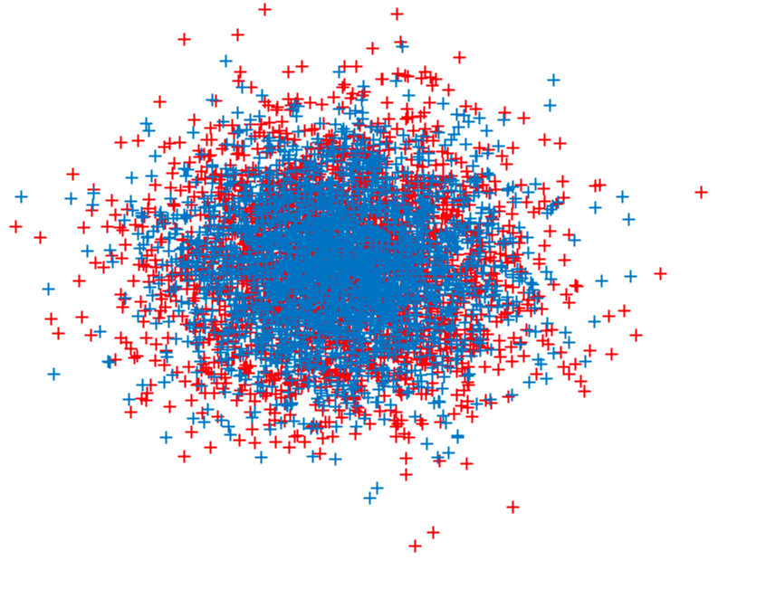
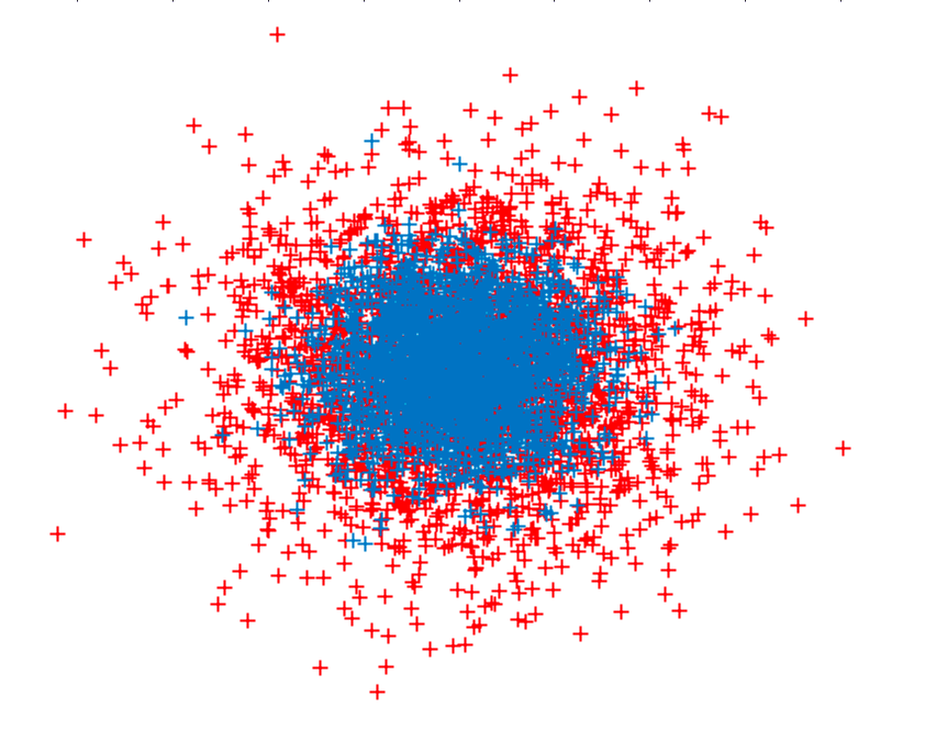
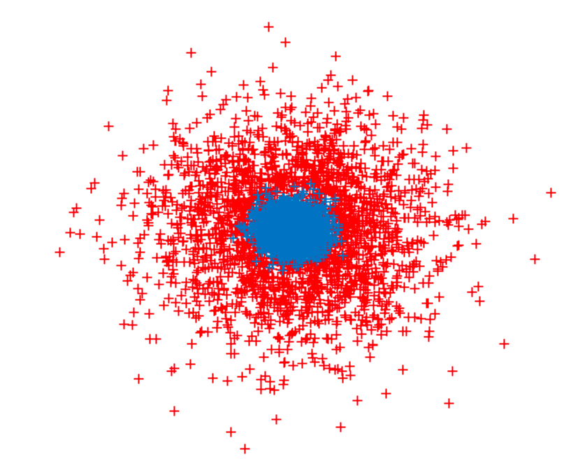
In Figure 1, we show the i.i.d. samples from the distributions P𝑽P_{\bm{V}} and P𝑾P_{\bm{W}} for different choices of variance parameter of λ=0.1\lambda=0.1, λ=0.5\lambda=0.5, and λ=0.9\lambda=0.9. Notice that for larger λ\lambda the divergence is reduced and thus performing the two-sample test is more difficult. From Figure 1, we clearly observe that for large values of λ\lambda, the data-points from the two distributions P𝑽P_{\bm{V}} and P𝑾P_{\bm{W}} have a large overlap and conducting a statistical test to distinguish between these two distributions is more challenging.

4.1.1. Kernel Learning Approach

Figure 4 depicts our two-phase kernel learning procedure. The kernel learning approach consists of training the auto-encoder for the dimensionality reduction and the kernel optimization sequentially, i.e.,

(4.9) supμ^N∈𝒫Nsupι∈𝒬MMD^Kμ^N∘ια​[P𝑽,P𝑾].\displaystyle\sup_{\widehat{\mu}^{N}\in\mathcal{P}^{N}}\sup_{\iota\in\mathcal{Q}}\widehat{\mathrm{MMD}}_{K_{\widehat{\mu}^{N}}\circ\iota}^{\alpha}[P_{\bm{V}},P_{\bm{W}}].

where the function class is defined 𝒬={ι(𝒛)=σ(𝚺𝒛+𝒃),𝚺∈d0×d,𝒃∈d0}\mathcal{Q}\mathrel{{\mathop{=}\limits}}\{\iota(\bm{z})=\sigma(\bm{\Sigma}\bm{z}+\bm{b}),\bm{\Sigma}\in\real^{d_{0}\times d},\bm{b}\in\real^{d_{0}}\}, and (Kμ^N∘ι)​(𝒙1,𝒙2)=Kμ^N​(ι⁡(𝒙1),ι⁡(𝒙2))(K_{\widehat{\mu}^{N}}\circ\iota)(\bm{x}_{1},\bm{x}_{2})=K_{\widehat{\mu}^{N}}(\iota(\bm{x}_{1}),\iota(\bm{x}_{2})). Here, 𝝈⁡(⋅)\bm{\sigma}(\cdot) is the sigmoid non-linearity. Now, we consider a two-phase optimization procedure:

  • •

    Phase (I): we fix the kernel function, and optimize the auto-encoder to compute a co-variance matrix 𝚺\bm{\Sigma} and the bias term 𝒃\bm{b} for the dimensionality reduction.

  • •

    Phase (II): we optimize the kernel based from the learned embedded features ι⁡(𝒙)\iota(\bm{x}).

This two-phase procedure significantly improves the computational complexity of SGD as it reduces the dimensionality of random feature samples 𝝃∈D\bm{\xi}\in\real^{D}, D=d0≪dD=d_{0}\ll d.

Refer to caption
Refer to caption
Refer to caption

(a)                  (b)                  (c)

Figure 1. Visualization of data-points using the synthetic data generation models with multivariate Gaussian distributions P𝑽=𝖭⁡(𝟎,(1+λ)​𝑰d×d)P_{\bm{V}}=\mathsf{N}(\bm{0},(1+\lambda)\bm{I}_{d\times d}) and P𝑾=𝖭⁡(𝟎,(1−λ)​𝑰d×d)P_{\bm{W}}=\mathsf{N}(\bm{0},(1-\lambda)\bm{I}_{d\times d}) for d=2d=2. Panel (a): λ=0.1\lambda=0.1, Panel (b): λ=0.5\lambda=0.5, and Panel (c): λ=0.9\lambda=0.9.

4.1.2. Statistical Hypothesis Testing with the Kernel MMD

Let 𝑽1,⋯,𝑽m∼i.i.d.P𝑽=𝖭(𝟎,(1+λ)𝑰d×d)\bm{V}_{1},\cdots,\bm{V}_{m}\sim_{\text{i.i.d.}}P_{\bm{V}}=\mathsf{N}(\bm{0},(1+\lambda)\bm{I}_{d\times d}), and 𝑾1,⋯,𝑾n∼i.i.d.P𝑾=𝖭(𝟎,(1−λ)𝑰d×d)\bm{W}_{1},\cdots,\bm{W}_{n}\sim_{\text{i.i.d.}}P_{\bm{W}}=\mathsf{N}(\bm{0},(1-\lambda)\bm{I}_{d\times d}). Given these i.i.d. samples, the statistical test 𝒯⁡({𝑽i}i=1m,{𝑾i}j=1n):𝒱m×𝒲n→{0,1}\mathcal{T}(\{\bm{V}_{i}\}_{i=1}^{m},\{\bm{W}_{i}\}_{j=1}^{n}):\mathcal{V}^{m}\times\mathcal{W}^{n}\rightarrow\{0,1\} is used to distinguish between these hypotheses:

  • •

    Null hypothesis 𝖧0:P𝑽=P𝑾\mathsf{H}_{0}:P_{\bm{V}}=P_{\bm{W}} (thus λ=0\lambda=0),

  • •

    Alternative hypothesis 𝖧1:P𝑽≠P𝑾\mathsf{H}_{1}:P_{\bm{V}}\not=P_{\bm{W}} (thus λ>0\lambda>0).

To perform hypothesis testing via the kernel MMD, we require that ℋ𝒳\mathcal{H}_{\mathcal{X}} is a universal RKHS, defined on a compact metric space 𝒳\mathcal{X}. Universality requires that the kernel K⁡(⋅,⋅)K(\cdot,\cdot) be continuous and, ℋ𝒳\mathcal{H}_{\mathcal{X}} be dense in C⁡(𝒳)C(\mathcal{X}). Under these conditions, the following theorem establishes that the kernel MMD is indeed a metric:

Theorem 4.1.

(Metrizablity of the RKHS) Let ℱ\mathcal{F} denotes a unit ball in a universal RKHS ℋ𝒳\mathcal{H}_{\mathcal{X}} defined on a compact metric space 𝒳\mathcal{X} with the associated continuous kernel K⁡(⋅,⋅)K(\cdot,\cdot). Then, the kernel MMD is a metric in the sense that MMDK​[P𝐕,P𝐖]=0\mathrm{MMD}_{K}[P_{\bm{V}},P_{\bm{W}}]=0 if and only if P𝐕=P𝐖P_{\bm{V}}=P_{\bm{W}}.

A radial kernel is universal if the support of the measure in the integral representation in Eq. (2.9) excludes the origin, i.e., supp⁡(μ)≠{0}\mathrm{supp}(\mu)\not=\{0\}, see [53].

To design a test, let μ^mN​(𝝃)=1N​∑k=1Nδ⁡(𝝃−𝝃mk)\widehat{\mu}^{N}_{m}(\bm{\xi})={1\over N}\sum_{k=1}^{N}\delta(\bm{\xi}-\bm{\xi}_{m}^{k}) denotes the solution of SGD in (4.7) for solving the optimization problem. Consider the following MMD estimator consisting of two UU-statistics and an empirical function

MMD^Kμ^mN∘ι​[{𝑽i}i=1m,{𝑾i}i=1n]\displaystyle\widehat{\mathrm{MMD}}_{K_{\widehat{\mu}_{m}^{N}}\circ\iota}\big[\{\bm{V}_{i}\}_{i=1}^{m},\{\bm{W}_{i}\}_{i=1}^{n}\big] =1m⁡(m−1)​∑k=1N∑i≠jφ⁡(ι⁡(𝑽i),𝝎mk)​φ​(ι⁡(𝑽j),𝝎mk)\displaystyle=\dfrac{1}{m(m-1)}\sum_{k=1}^{N}\sum_{i\not=j}\varphi(\iota(\bm{V}_{i}),\bm{\omega}_{m}^{k})\varphi(\iota(\bm{V}_{j}),\bm{\omega}_{m}^{k})
+1n⁡(n−1)∑k=1N∑i≠jφ(ι(𝑾i),𝝎mk)φ(ι(𝑾j),𝝎mk)\displaystyle\hskip 11.38109pt+\dfrac{1}{n(n-1)}\sum_{k=1}^{N}\sum_{i\not=j}\varphi(\iota(\bm{W}_{i}),\bm{\omega}_{m}^{k})\varphi(\iota(\bm{W}_{j}),\bm{\omega}_{m}^{k})
(4.10) −2n​m∑k=1N∑i=1m∑j=1nφ(ι(𝑾i),𝝎mk)φ(ι(𝑽j),𝝎mk).\displaystyle\hskip 11.38109pt-\dfrac{2}{nm}\sum_{k=1}^{N}\sum_{i=1}^{m}\sum_{j=1}^{n}\varphi(\iota(\bm{W}_{i}),\bm{\omega}_{m}^{k})\varphi(\iota(\bm{V}_{j}),\bm{\omega}^{k}_{m}).

Given the samples {𝑽i}i=1m\{\bm{V}_{i}\}_{i=1}^{m} and {𝑾i}i=1n\{\bm{W}_{i}\}_{i=1}^{n}, we design a test statistic as below

(4.11) 𝒯⁡({𝑽i}i=1m,{𝑾i}i=1n)={𝖧0if ​MMD^Kμ^mN∘ι​[{𝑽i}i=1m,{𝑾i}i=1n]≤τ𝖧1if ​MMD^Kμ^mN∘ι​[{𝑽i}i=1m,{𝑾i}i=1n]>τ,.\displaystyle\mathcal{T}(\{\bm{V}_{i}\}_{i=1}^{m},\{\bm{W}_{i}\}_{i=1}^{n})\mathrel{{\mathop{=}\limits}}\begin{cases}\mathsf{H}_{0}&\text{if }\widehat{\mathrm{MMD}}_{K_{\widehat{\mu}_{m}^{N}}\circ\iota}\big[\{\bm{V}_{i}\}_{i=1}^{m},\{\bm{W}_{i}\}_{i=1}^{n}\big]\leq\tau\\ \mathsf{H}_{1}&\text{if }\widehat{\mathrm{MMD}}_{K_{\widehat{\mu}_{m}^{N}}\circ\iota}\big[\{\bm{V}_{i}\}_{i=1}^{m},\{\bm{W}_{i}\}_{i=1}^{n}\big]>\tau,\end{cases}.

where τ∈\tau\in\real is a threshold. Notice that the unbiased MMD estimator of (4.10) can be negative despite the fact that the population MMD is non-negative. Consequently, negative values for the statistical threshold τ\tau (4.11) are admissible. Nevertheless, int our simulations, we only consider non-negative values for the threshold τ\tau.

A Type I error is made when 𝖧0\mathsf{H}_{0} is rejected based on the observed samples, despite the null hypothesis having generated the data. Conversely, a Type II error occurs when 𝖧0\mathsf{H}_{0} is accepted despite the alternative hypothesis 𝖧1\mathsf{H}_{1} being true. The significance level α\alpha of a test is an upper bound on the probability of a Type I error: this is a design parameter of the test which must be set in advance, and is used to determine the threshold to which we compare the test statistic. The power of a test is the probability of rejecting the null hypothesis 𝖧0\mathsf{H}_{0} when it is indeed incorrect. In particular,

(4.12) Power=I​P​(reject​𝖧0|𝖧1​is true).\displaystyle\mathrm{Power}\mathrel{{\mathop{=}\limits}}{\rm I\!P}(\text{reject}\ \mathsf{H}_{0}|\mathsf{H}_{1}\ \text{is true}).

In this sense, the statistical power controls the probability of making Type II errors.

4.2. Empirical results on benchmark data-sets

In Figure 4, we evaluate the power of the test for 100100 trials of hypothesis test using the test statistics of (4.11). To obtain the result, we used an autoencoder to reduce the dimension from d=100d=100 to p=50p=50. Clearly, for the trained kernel in Panel (a) of Figure 4, the threshold τ\tau for which Power=1\mathrm{Power}=1 increases after learning the kernel via the two phase procedure described earlier. In comparison, in Panel (b), we observe that training an auto-encoder only with a fixed standard Gaussian kernel K⁡(𝒙,𝒚)=exp⁡(−‖𝒙−𝒚‖22)K(\bm{x},\bm{y})=\exp(-\|\bm{x}-\bm{y}\|_{2}^{2}) attains lower thresholds compared to our two-phase procedure. In Panel (c), we demonstrate the case of a fixed Gaussian kernel without an auto-encoder. In this case, the threshold is significantly lower due to the large dimensionality of the data. We also observer that the particle SGD for optimization we proposed in [26] to optimize the translation invariant kernels provides the highest statistical power for a given threshold value. Nevertheless, as we observe in Figure 4, the run-time of the particle SGD for a given number of particles is significantly higher than Algorithm 1. This is due to the fact that the dimension of the particles in the particle SGD is dependent on the number of hidden layers of auto-encoder. In contrast, the particles in Algorithm 1 are one dimensional.

Refer to caption
Refer to caption
Refer to caption
Refer to caption

(a)                (b)               (c)               (d)

Figure 2. The statistical power versus the threshold τ\tau for the binary hypothesis testing via the unbiased estimator of the kernel MMD. The parameters for this simulations are λ∈{0.1,0.5,0.9}\lambda\in\{0.1,0.5,0.9\}, d=100d=100, d0=50d_{0}=50, n+m=100n+m=100, and N=5000N=5000. Panel (a): Trained radial kernel using the two-phase procedure with the particle Langevin optimization in Algorithm 1, and an auto-encoder, Panel (b): Trained shift-invariant kernel using particle SGD in Eq. (4.7) and an auto-encoder, Panel (c): Trained kernel with an auto-encoder and a fixed Gaussian kernel whose the bandwidth is σ=1\sigma=1, Panel (d): Untrained kernel without an auto-encoder.
Refer to caption
Refer to caption
Refer to caption
Refer to caption

(a)                (b)               (c)               (d)

Refer to caption
Refer to caption
Refer to caption
Refer to caption

(e)                (f)               (g)               (h)

Figure 3. The evolution of the histogram of Langevin particles ξ1,⋯,ξN∈Ξ=+\xi^{1},\cdots,\xi^{N}\in\Xi=\real_{+} and predictions from the theory (Theorem 3.2) with γ=10000\gamma=10000, R=10000R=10000, η=10−5\eta=10^{-5}. Panel (a): m=10​(t=10−4​s)m=10\ (t=10^{-4}s), Panel (b): m=1000​(t=0.1​s)m=1000(t=0.1s), Panel (c):m=5000​(t=0.5​s)m=5000\ (t=0.5s), Panel (d): m=10000​(t=1​s)m=10000(t=1s), Panel (e): m=50000​(t=5​s)m=50000\ (t=5s), Panel (f):m=100000​(t=10​s)m=100000\ (t=10s), Panel (g): m=200000​(t=20​s)m=200000\ (t=20s), Panel (h): am=300000​(t=30​s)m=300000\ (t=30s).

5. Application to Locally Sensitive Hashing

Refer to caption
Refer to caption
Refer to caption

(a)                (b)                 (c)

Refer to caption
Refer to caption
Refer to caption

(d)                (e)               (f)

Figure 4. The scatter plots of the normalized Hamming distance versus Euclidean distance for the locally sensitive hash function of Lemma 5.2. The hash functions are generated with the random features associated with an untrained Gaussian kernel with the bandwidth parameter of σ=1\sigma=1 (top row), and a trained kernel with Algorithm 1 in conjunction with a kk-mean clustering method (bottom row). Panels (a),(d): 128 bits, Panels (b),(e): 512 bits, Panels (c),(f): 4096 bits.
Refer to caption
Refer to caption
Refer to caption

(a)                 (b)                  (c)

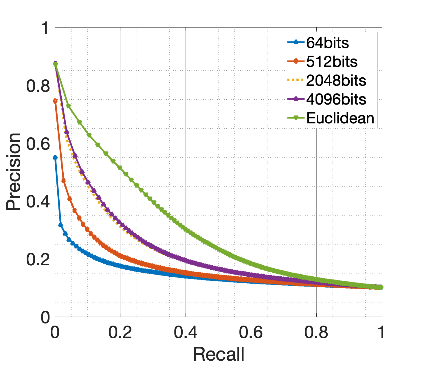
Figure 5. The precision-recall curves for the kernel locally sensitive hashing. Panel (a): hash function Fn:𝒳→ℤ2nF^{n}:\mathcal{X}\rightarrow\mathbb{Z}_{2}^{n} of Lemma 5.2 with an untrained Gaussian kernel, Panel (b): hash function Fn:𝒳→ℤ2nF^{n}:\mathcal{X}\rightarrow\mathbb{Z}_{2}^{n} of Lemma 5.2 with the trained kernel with Algorithm 1, where the labeled data for kernel training is generated via the kk-mean clustering with k=10k=10, and one versus all rule. Panel (c): hash function Gn:𝒳→ℤqnG^{n}:\mathcal{X}\rightarrow\mathbb{Z}_{q}^{n} of Lemma 5.3 with the quantization levels q∈{2,3,5,10}q\in\{2,3,5,10\}, and the fixed code-word length of n=512n=512.
Refer to caption
Refer to caption
Refer to caption

(a)               (b)                (c)

Figure 6. The (normalized) histogram of the (rescaled) Lee distance (red color) and the (rescaled) Euclidean distance (blue color) of a sample query point from each point of the MNIST data-base for different quantization level qq in Lemma 5.3, Panel (a): q=2q=2, Panel (b): q=20q=20, Panel (c): q=50q=50. Increasing the quantization level qq in the Lee distance yields a more fine grained approximation for the Euclidean distance. (best viewed in color)
Refer to caption
Refer to caption
Refer to caption

(a)             (b)            (c)

Refer to caption
Refer to caption
Refer to caption

(d)             (e)            (f)

Refer to caption
Refer to caption
Refer to caption

(g)             (h)            (i)

Refer to caption
Refer to caption
Refer to caption

(j)             (k)            (l)

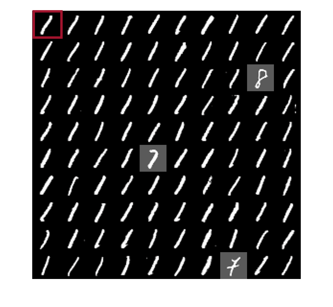
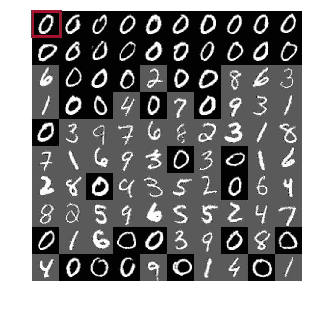
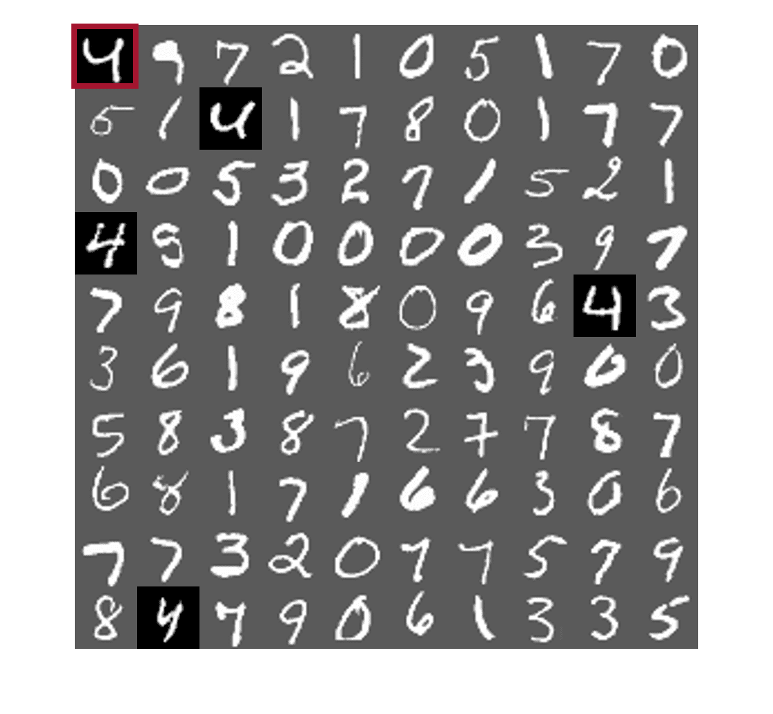
Figure 7. Image retrieval for three query digits {1,0,4}\{1,0,4\} on the MNIST database. The query image is in the top left of the collage (red box), and the incorrect retrieved images are shaded with the gray color. The Panels (a)-(c): Euclidean distance. Panels (d)-(f): ℤ2n\mathbb{Z}_{2}^{n} code with an untrained kernel and n=4096n=4096 bits. Panels (g)-(i): ℤ2n\mathbb{Z}_{2}^{n} code with a trained kernel with Algoirthm 1 and n=4096n=4096. Panels (j)-(l): ℤqn\mathbb{Z}_{q}^{n} codeword length with q=10q=10 and n=1024n=1024. (best viewed in color)

The research on computer systems and web search in the mid-nineties was focused on designing “hash” functions that were sensitive to the topology on the input domain, and preserved distances approximately during hashing. Constructions of such hash functions led to efficient methods to detect similarity of files in distributed file systems and proximity of documents on the web. We describe the problem and results below. Recall that a metric space (𝒞,d)(\mathcal{C},d) is given by a set 𝒞\mathcal{C} (here the set of cells) and a distance measure d:𝒳×𝒳→+d:\mathcal{X}\times\mathcal{X}\rightarrow\real_{+} which satisfies the axioms of being a metric.

Definition 5.1.

(Locally Sensitive Hash Function) Given a metric space (𝒞,ρ)(\mathcal{C},\rho) and the set ℒ\mathcal{L}, a family of function H⊆{h:𝒞→ℒ}H\subseteq\{h:\mathcal{C}\rightarrow\mathcal{L}\} is said to be a basic locality sensitive hash (LSH) family if there exists an increasing invertible function α:+→[0,1]\alpha:\real_{+}\rightarrow[0,1] such that for all 𝒙,𝒙~∈𝒳\bm{x},\tilde{\bm{x}}\in\mathcal{X}, we have

(5.1) IPh∈ℋ[h(𝒙)=h(𝒙~)]≤α(d(𝒙,𝒙~)).\displaystyle{\rm I\!P}_{h\in\mathcal{H}}[h(\bm{x})=h(\tilde{\bm{x}})]\leq\alpha(d(\bm{x},\tilde{\bm{x}})).

To contrast the locally sensitive hash functions with the standard hash function families note that in the latter, the goal is to map a domain 𝒞\mathcal{C} to a range ℒ\mathcal{L} such that the probability of a collision among any pair of elements 𝒙≠𝒙~∈𝒞\bm{x}\not=\tilde{\bm{x}}\in\mathcal{C} is small. In contrast, with LSH families, we wish for the probability of a collision to be small only when the pairwise distance d⁡(𝒙,𝒙~)d(\bm{x},\tilde{\bm{x}}) is large, and we do want a high probability of collision when d⁡(𝒙,𝒙~)d(\bm{x},\tilde{\bm{x}}) is small. Indyk and Motwani [22] showed that such a hashing scheme facilitates the construction of efficient data structures for answering approximate nearest-neighbor queries on the collection of objects.

In the sequel, we describe a family of locally sensitive hash functions due to Raginsky, et al. [40], where the measure d⁡(𝒙,𝒙~)d(\bm{x},\tilde{\bm{x}}) is determined by a kernel function. We draw a random threshold t∼Uniform⁡[−1,1]t\sim\mathrm{Uniform}[-1,1] and define the quantizer Qt​(u)=sgn⁡(t+u)Q_{t}(u)=\mathrm{sgn}(t+u). The following theorem is due to Raginsky, et al. [40]:

Lemma 5.2.

(Kernel Hash Function, Raginsky, et al. [40]) Consider a translation invariant kernel K:𝒳×𝒳→,K⁡(𝐱,𝐱~)=ϕ⁡(𝐱−𝐱~)K:\mathcal{X}\times\mathcal{X}\rightarrow\real,K(\bm{x},\tilde{\bm{x}})=\phi(\bm{x}-\tilde{\bm{x}}). Define the following hamming ℤ2n\mathbb{Z}_{2}^{n}-code

(5.2) Fn​(𝒙)=(Ft1,b1,𝝎1​(𝒙),⋯,Fτn,bn,𝝎n​(𝒙)),\displaystyle F^{n}(\bm{x})\mathrel{{\mathop{=}\limits}}(F_{t_{1},b_{1},\bm{\omega}_{1}}(\bm{x}),\cdots,F_{\tau_{n},b_{n},\bm{\omega}_{n}}(\bm{x})),

where (bi)1≤i≤n∼i.i.dUniform[−π,π](b_{i})_{1\leq i\leq n}\sim_{\text{i.i.d}}\mathrm{Uniform}[-\pi,\pi], (ti)1≤i≤n∼i.i.d.Uniform[−1,1](t_{i})_{1\leq i\leq n}\sim_{\text{i.i.d.}}\mathrm{Uniform}[-1,1], and (𝛚i)1≤i≤n∼i.i.d.ν(\bm{\omega}_{i})_{1\leq i\leq n}\sim_{\text{i.i.d.}}\nu, where ν\nu is the distribution in the Rahimi and Recht random feature model

(5.3) ϕ(𝒙−𝒙~)=∫dφ(𝒙;𝝎)φ(𝒙~;𝝎)dν(𝝎).\displaystyle\phi(\bm{x}-\tilde{\bm{x}})=\int_{\real{}^{d}}\varphi(\bm{x};\bm{\omega})\varphi(\tilde{\bm{x}};\bm{\omega})\mathrm{d}\nu(\bm{\omega}).

Furthermore, Ft,b,𝛚:d→ℤ2F_{t,b,\bm{\omega}}:\real^{d}\rightarrow\mathbb{Z}_{2} is a mapping defined as follows

(5.4) Ft,b,𝝎​(𝒙)=12​[1+Qt​(cos⁡(⟨𝝎,𝒙⟩+b))].\displaystyle F_{t,b,\bm{\omega}}(\bm{x})\mathrel{{\mathop{=}\limits}}\dfrac{1}{2}\Big[1+Q_{t}(\cos(\langle\bm{\omega},\bm{x}\rangle+b))\Big].

Fix ϵ,δ∈(0,1)\epsilon,\delta\in(0,1). For any finite data set D={𝐱1,⋯,𝐱N}⊂dD=\{\bm{x}_{1},\cdots,\bm{x}_{N}\}\subset\real^{d}, FnF^{n} is such that

(5.5) hK​(𝒙i−𝒙j)−δ≤1n​dH​(Fn​(𝒙i),Fn​(𝒙j))≤hK​(𝒙i−𝒙j)+δ,\displaystyle h_{K}(\bm{x}_{i}-\bm{x}_{j})-\delta\leq{1\over n}d_{\mathrm{H}}(F^{n}(\bm{x}_{i}),F^{n}(\bm{x}_{j}))\leq h_{K}(\bm{x}_{i}-\bm{x}_{j})+\delta,

where dH​(⋅,⋅):ℤ2n×ℤ2n→{0,1}d_{H}(\cdot,\cdot):\mathbb{Z}^{n}_{2}\times\mathbb{Z}^{n}_{2}\rightarrow\{0,1\} is the Hamming distance. Furthermore,

(5.6) hK​(𝒙i−𝒙j)=8π2​∑m=0∞1−K⁡(m​𝒙i−m​𝒙~i)4​m2−1.\displaystyle h_{K}(\bm{x}_{i}-\bm{x}_{j})\mathrel{{\mathop{=}\limits}}\dfrac{8}{\pi^{2}}\sum_{m=0}^{\infty}\dfrac{1-K(m\bm{x}_{i}-m\tilde{\bm{x}}_{i})}{4m^{2}-1}.

The construction of LSH in Eq. (5.4) of Lemma (5.2) is based on the random feature model of Rahimi and Recht [41, 42], and is restricted to the Hamming codes defined on a hyper-cube. In the sequel, we present an alternative kernel LSH using the embedding of functions in Lp​(Ω,ν)L^{p}(\Omega,\nu) space into ℓp\ell^{p}-spaces, generalizing the result of Lemma 5.2 to any finite integer alphabet ℤq={0,1,⋯,q−1}\mathbb{Z}_{q}\mathrel{{\mathop{=}\limits}}\{0,1,\cdots,q-1\}. To describe the result, we define the Lee distance between two code-words 𝒙=(x1,⋯,xn),𝒚=(y1,⋯,yn)∈ℤqn\bm{x}=(x_{1},\cdots,x_{n}),\bm{y}=(y_{1},\cdots,y_{n})\in\mathbb{Z}_{q}^{n} of length nn as follows

(5.7a) dLee​(𝒙,𝒚)\displaystyle d_{\mathrm{Lee}}(\bm{x},\bm{y}) =∑i=1nmin⁡{(xi−yi)​mod​q,(yi−xi)​mod​q}\displaystyle\mathrel{{\mathop{=}\limits}}\sum_{i=1}^{n}\min\{(x_{i}-y_{i})\ \mathrm{mod}\ q,(y_{i}-x_{i})\ \mathrm{mod}\ q\}
(5.7b) =∑i=1nmin⁡{|yi−xi|,q−|yi−xi|}.\displaystyle=\sum_{i=1}^{n}\min\{|y_{i}-x_{i}|,q-|y_{i}-x_{i}|\}.

In the special cases of q=2q=2 and q=3q=3, the Lee distance corresponds to the Hamming distance as distances are 00 for two single equal symbols and 1 for two single non-equal symbols. For q>3q>3 this is not the case anymore, and the Lee distance can become larger than one.

Lemma 5.3.

(Generalized Kernel LSH) Consider a translation invariant kernel K:d×d→,K(𝐱,𝐱~)=ψ(∥𝐱−𝐱~∥22)K:\real^{d}\times\real^{d}\rightarrow\real,K(\bm{x},\tilde{\bm{x}})=\psi(\|\bm{x}-\tilde{\bm{x}}\|_{2}^{2}). Define a random map Gt,𝛚:d→ℤqG_{t,\bm{\omega}}:\real^{d}\rightarrow\mathbb{Z}_{q} through the following function

(5.8) Gt,𝒘​(𝒙)=⌈q−1​(⟨𝒘,𝝋N​(𝒙)⟩+t)⌉​mod​q,\displaystyle G_{t,\bm{w}}(\bm{x})\mathrel{{\mathop{=}\limits}}\left\lceil q^{-1}({\langle\bm{w},\bm{\varphi}_{N}(\bm{x})\rangle+t})\right\rceil\mathrm{mod}\ q,

where 𝐰∼𝖭⁡(0,𝐈N×N)\bm{w}\sim\mathsf{N}(0,\bm{I}_{N\times N}), t∼Uniform⁡[0,q]t\sim\mathrm{Uniform}[0,q]. Moreover, 𝛗N​(𝐱)=(cos⁡(⟨𝛚k,𝐱⟩+bk))1≤k≤N\bm{\varphi}_{N}(\bm{x})\mathrel{{\mathop{=}\limits}}(\cos(\langle\bm{\omega}_{k},\bm{x}\rangle+b_{k}))_{1\leq k\leq N}, where b1,⋯,bN∼i.i.d.ν0=Uniform[−π,π]b_{1},\cdots,b_{N}\sim_{\text{i.i.d.}}\nu_{0}\mathrel{{\mathop{=}\limits}}\mathrm{Uniform}[-\pi,\pi], and 𝛚1,⋯,𝛚N∼i.i.d.ν\bm{\omega}_{1},\cdots,\bm{\omega}_{N}\sim_{\text{i.i.d.}}\nu. Then, the probability of collision is bounded as follows

|IP[Gt,𝒘(𝒙)=Gt,𝝎(𝒙~)]−Ψq(K(𝒙,𝒙~))|=𝒪(ln⁡(N)N).\displaystyle\left|{\rm I\!P}\Big[G_{t,\bm{w}}(\bm{x})=G_{t,\bm{\omega}}(\tilde{\bm{x}})\Big]-\Psi_{q}(K(\bm{x},\tilde{\bm{x}}))\right|=\mathcal{O}\left(\dfrac{\ln(N)}{N}\right).

where Ψq:+↦+\Psi_{q}:\real_{+}\mapsto\real_{+} is defined

(5.9) Ψq​(u)=∫0q1π⁡(1−u)​e−s24​(1−u)​(1−sq)​𝑑s.\displaystyle\Psi_{q}(u)\mathrel{{\mathop{=}\limits}}\int_{0}^{q}{1\over\sqrt{\pi(1-u)}}e^{-{s^{2}\over 4(1-u)}}\left(1-\dfrac{s}{q}\right)\mathrm{d}s.

The proof of Lemma 5.3 is presented in Appendix A.12, and uses the property of the stable distributions.

5.1. Description of the experiment

We present image retrieval results for 10000 images from MNIST databases [10]. The images are 28 by 28 pixels and are compressed via an auto-encoder with 500 hidden layers, which have proven to be effective at learning useful features. For this experiment, we randomly select 1,000 images to serve as queries, and the remaining 9,000 images make up the “database”. To distinguish true positives from false positives for the performance evaluation retrieval performance, we select a “nominal” neighborhood.

5.2. Results

In Figure 4, we illustrate the scatter plots of the hash codes Fn​(𝒙)F^{n}(\bm{x}) of length n∈{128,512,4096}n\in\{128,512,4096\} bits. In Figure 4 (a)-(c), we show the scatter plots for Hamming codes constructed by Lemma 5.2 using an untrained Gaussian kernel K⁡(𝒙,𝒙^)=exp⁡(−‖𝒙−𝒙^‖22)K(\bm{x},\widehat{\bm{x}})=\exp(-\|\bm{x}-\widehat{\bm{x}}\|_{2}^{2}). From Figure 4 (a)-(c) we observe that as the number of bits of the Hamming code increase, the scatter plots concentrate around a curve that has a flat region. Evidently, this curve deviates from the ideal curve which is a straight line passing through the origin. In particular, in 4 (a)-(c), as the Euclidean distance changes on the interval [2,8][2,8] of xx-axis, the normalized Hamming distance of the constructed codes remains constant.

To attain proportionality between the Hamming distance and the Euclidean distance, we train the kernel using Algorithm 1. To generate the labels for kernel training, we first perform a kk-NN on 1000 images from 9,000 images of the data-base, where here k=10k=10. Then, we generate the binary class labels by assigning y=+1y=+1 to the points in a randomly chosen cluster, and y=−1y=-1 to the remaining data-points in other clusters (i.e., the one-versus-all rule). After training the kernel, the kernel is used to generate the Hash codes using the construction of Lemma 5.2. The resulting scattering plots are depicted in Figure 4 (d)-(f), and the Hamming distances are more proportional to the Euclidean distance.

Central to our study is the precision-recall curve, which captures the trade-off between precision and recall for different threshold. A high area under the curve represents both high recall and high precision, where high precision relates to a low false positive rate, and high recall relates to a low false negative rate. High scores for both show that the classifier is returning accurate results (high precision), as well as returning a majority of all positive results (high recall). Specifically,

(5.10a) Precision=|{relevant images}∩{retrieved images}||{retrieved images}|,\displaystyle{\displaystyle{\text{Precision}}\mathrel{{\mathop{=}\limits}}{\frac{|\{{\text{relevant images}}\}\cap\{{\text{retrieved images}}\}|}{|\{{\text{retrieved images}}\}|}}},
(5.10b) Recall=|{relevant images}∩{retrieved images}||{relevant images}|.\displaystyle{\displaystyle{\text{Recall}}\mathrel{{\mathop{=}\limits}}{\frac{|\{{\text{relevant images}}\}\cap\{{\text{retrieved images}}\}|}{|\{{\text{relevant images}}\}|}}}.

In Figure 5 we illustrate the precision-recall curves for Hamming codes of different lengths n∈{64,512,2048,4096}n\in\{64,512,2048,4096\}. We also depict the precision-recall curve for the Euclidean distance. We recall the notions of the recall and precision as follows From Figure 5(a), we depict the precision-recall curves for Hamming codes constructed from the Gaussian kernel. We observe that even Hamming codes of length 40964096 bits attain the precision-recall curve that is significantly lower than the Euclidean curve. In Figure 5(b), we illustrate the precision-recall curves after training kernels using Algorithm 1. The curves from Hamming codes are markedly closer to the curve associated with the Euclidean distance. In Figure 5(c), we depict the precision-recall curves using the qq-ary codes in Lemma 5.3 for different quantization levels q∈{2,3,5,10}q\in\{2,3,5,10\}. Clearly, increasing qq leads to a better performance initially while larger values of qq has a diminishing return. This can be justified using Figure 6, where we plot the normalized histogram of the distance of a sample query point from each point of the MNIST data-base consisting of 9,000 of data-points. The blue color histogram depict the histogram using a Euclidean distance, and the orange color histogram with spikes depicts the histogram of the Lee distance. Figure 6(a)-(c) are plotted with the quantization levels q=2q=2, q=20q=20, and q=50q=50, respectively. As the quantization level increases, the histogram of the Lee distance provides a better approximation for the Euclidean distance histogram. However, even for large qq, there is a disparity between the two histograms, as the length of the qq-ary codes are fixed at n=512n=512 and is finite.

In Figure 7, we depict the retrieval results for three query digits {1,0,4}\{1,0,4\} on MNIST data-set. In Fig. 7(a)-(c), we show the performance of retrieval system using a Euclidean distance for searching nearest neighbor. In particular, for each query digit, the retrieval system returns 99 similar images among 9,000 images in the data-base using nearest neighborhood search. The retrieved images for less challenging digits such as 1 and 0 are all correct, while for more challenging query points such as 4, some erroneous images are retrieved. In Fig. 7(d)-(f), we depict the retrieved images using a Hamming distance for the nearest neighborhood search, where the Hamming codes for each feature vector are generated via the kernel LSH in Lemma 5.2, where a Gaussian kernel K⁡(𝒙,𝒙^)=exp⁡(−‖𝒙−𝒙^‖22)K(\bm{x},\widehat{\bm{x}})=\exp(-\|\bm{x}-\widehat{\bm{x}}\|_{2}^{2}) is employed. We observe that compared to the Euclidean distance in Fig. 7(a)-(c), the performance of Hamming based nearest neighbor search is significantly less accurate. However, we point out that from a computation complexity perspective, computing the Hamming distance is significantly more efficient than the Euclidean distance which is the main motivation in using LSH for nearest neighborhood search.

In Fig. 7 (g)-(i), we show the retrieval results after training the kernel using Algorithm 1. Clearly, the retrievals are more accurate on the digits 00 and 44. However, the length of the Hamming code required to achieve such performance is quite large n=4096n=4096. In Fig. 7 (j)-(l), we show the retrieval performance using the qq-ary code of length n=1024n=1024 and the quanitization level of q=10q=10. Although the length of the qq-ary code is significantly smaller than that of the Hamming code, the retrieval error is slightly less. However, the computational cost is slightly higher than that of the Hamming code.

In the future, we will test our method on data-sets consisting of millions of data points. At present, our promising initial results on MNIST data-set, combined with our comprehensive theoretical analysis, convincingly demonstrate the potential usefulness of our kernel learning scheme for large-scale indexing and search applications.

6. Classification on Benchmark Data-Sets

We now apply our kernel learning method for classification and regression tasks on real-world data-sets.

6.1. Data-Sets Description

We apply our kernel learning approach to classification and regression tasks of real-world data-sets. In Table 1, we provide the characteristics of each data-set. All of these datasets are publicly available at UCI repository.66 6 https://archive.ics.uci.edu/ml/index.php

6.1.1. Online news popularity

This data-set summarizes a heterogeneous set of features about articles published by Mashable in a period of two years. The goal is to predict the number of shares in social networks (popularity).

6.1.2. Buzz in social media dataset

This data-set contains examples of buzz events from two different social networks: Twitter, and Tom’s Hardware, a forum network focusing on new technology with more conservative dynamics

6.1.3. Adult

Adult data-set contains the census information of individuals including education, gender, and capital gain. The assigned classification task is to predict whether a person earns over 50K annually. The train and test sets are two separated files consisting of roughly 32000 and 16000 samples respectively.

6.1.4. Epileptic Seizure Detection

The epileptic seizure detection data-set consists of a recording of brain activity for 23.6 seconds. The corresponding time-series is sampled into 4097 data points. Each data point is the value of the EEG recording at a different point in time. So we have total 500 individuals with each has 4097 data points for 23.5 seconds. The 4097 data points are then divided and shuffled every into 23 segments, each segment contains 178 data points for 1 second, and each data point is the value of the EEG recording at a different point in time.

6.2. Quantitative Comparison

In Figure 9, we present the training and test results for regression and classification tasks on benchmark data-sets, using top d=35d=35 features from each data-set and for different number of random feature samples NN. In all the experiments, the SGD method provides a better accuracy in both the training and test phases. Nevertheless, in the case of seizure detection, we observe that for a small number of random feature samples, the importance sampling and Gaussian kernel with kkNN for bandwidth outperforms SGD.

In Figure 9, we illustrate the time consumed for training the kernel using SGD and importance sampling methods versus the number of random features NN. For the linear regression on Buzz, and Online news popularity the difference between the run-times are negligible. However, for classification tasks using Adult and Seizure, the difference in run-times are more pronounced.

Those visual observations are also repeated in a tabular form in Table 2, where the training and test errors as well algorithmic efficiencies (run-times) are presented for N=100N=100, N=1000N=1000, N=2000N=2000, and N=3000N=3000 number of features.

7. Conclusions

We have proposed and analyzed a distributionally robust optimization method to learn the distribution in the Schönberg integral representation of radial basis functions. In particular, we analyzed a projected particle Langevin dynamics to optimize the samples of the distribution in the integral representation of the radial kernels. We established theoretical performance guarantees for the proposed distributional optimization procedure. Specifically, we derived a non-asymptotic bound for the consistency of the finite sample approximations. Furthermore, using a mean-field analysis, we derived the scaling limits of a particle stochastic optimization method. We showed that in the scaling limits, the projected particle Langevin optimization converges to a reflected diffusion-drift process. We then derived a partial differential equation, describing the evolution of the law of the underlying reflected process. We evaluated the performance of the proposed kernel learning approach for classification on benchmark data-sets. We also used the kernel learning approach in conjunction with a kk-mean clustering method to train the kernel in the kernel locally sensitive hash functions.

Data-set Task dd ntrainingn_{\text{training}} ntestn_{\text{test}}
Buzz Regression 77 93800 46200
Online news popularity Regression 58 26561 13083
Adult Classification 122 32561 16281
Seizure Classification 178 8625 2875
Table 1. Description of the benchmark data-sets used in this paper.
Refer to caption
Refer to caption
Refer to caption
Refer to caption

(a)                (b)                 (c)                 (d)

Figure 8. Training and test errors of Algorithm 1 (black line), the SGD optimization (blue lines), the importance sampling (green lines), and a Gaussian kernel with the optimized bandwidth (red lines) for classification and linear regression tasks. The training and test errors are depicted with dashed and solid lines, respectively. Panel (a): Buzz, Panel (b): Online news popularity, Panel (c): Adult, Panel (d): Seizure. (Best viewed in color)
Refer to caption
Refer to caption
Refer to caption
Refer to caption

(a)                (b)                 (c)                 (d)

Figure 9. The run-times of kernel optimization algorithms using Algorithm 1, the SGD optimization, and Importance Sampling (IS). Panel (a): Buzz, Panel (b): Online news popularity, Panel (c): Adult, Panel (d): Seizure (Best viewed in color).
Buzz
Algorithm 1 NN=100 NN=1000 NN=2000 NN=3000
Training Error 0.448e−3-3 0.228e−3-3 0.781e−4-4 0.288e−3-3
Test Error 0.635e−3-3 0.554e−3-3 0.512e−3-3 0.397e−3-3
Run Time (sec) 0.160 0.748 1.454 1.867
Particle SGD NN=100 NN=1000 NN=2000 NN=3000
Training Error 0.501e−3-3 0.190e−3-3 0.180e−3-3 0.151e−3-3
Test Error 0.501e−3-3 0.190e−3-3 0.180e−3-3 0.151e−3-3
Run Time (sec) 0.316 1.971 4.617 14.621
Importance Sampling NN=100 NN=1000 NN=2000 NN=3000
Training Error 0.486e−3-3 0.466e−3-3 0.460e−3-3 0.455e−3-3
Test Error 0.677e−3-3 0.661e−3-3 0.662e−3-3 0.661e−3-3
Run Time (sec) 0.188 1.527 3.592 4.955
Gaussian Kernel NN=100 NN=1000 NN=2000 NN=3000
Training Error 0.484e−3-3 0.429e−3-3 0.379e−3-3 0.327e−3-3
Test Error 0.673e−3-3 0.673−3-3 0.709e−3-3 0.744e−3-3
Online news popularity
Algorithm 1 NN=100 NN=1000 NN=2000 NN=3000
Training Error 0.463e−3-3 0.239e−3-3 0.676e−3-3 0.288e−4-4
Test Error 0.654e−3-3 0.537e−3-3 0.474e−3-3 3.974e−4-4
Run Time (sec) 0.165 0.686 1.264 1.736
Particle SGD NN=100 NN=1000 NN=2000 NN=3000
Training Error 0.501e−3-3 0.190e−3-3 0.180e−3-3 0.151e−3-3
Test Error 0.687e−3-3 0.524e−3-3 0.567e−3-3 0.588e−3-3
Run Time (sec) 0.309 2.071 3.152 5.054
Importance Sampling NN=100 NN=1000 NN=2000 NN=3000
Training Error 0.486e−3-3 0.466e−3-3 0.460e−3-3 0.455e−3-3
Test Error 0.677e−3-3 0.662e−3-3 0.662e−3-3 0.661e−3-3
Run Time (sec) 0.222 1.640 4.254 10.782
Gaussian Kernel NN=100 NN=1000 NN=2000 NN=3000
Training Error 0.484e−3-3 0.429e−3-3 0.379e−3-3 0.327e−3-3
Test Error 0.673e−3-3 0.673e−3-3 0.709e−3-3 0.744e−3-3
Adult
Algorithm 1 NN=100 NN=1000 NN=2000 NN=3000
Training Error 0.221 0.201 0.199 0.199
Test Error 0.219 0.207 0.205 0.205
Run Time (sec) 0.155 0.645 1.426 1.802
Particle SGD NN=100 NN=1000 NN=2000 NN=3000
Training Error 0.240 0.204 0.199 0.197
Test Error 0.236 0.209 0.208 0.210
Run Time (sec) 0.274 1.784 9.272 11.295
Importance Sampling NN=100 NN=1000 NN=2000 NN=3000
Training Error 0.240 0.207 0.214 0.220
Test Error 0.236 0.219 0.222 0.223
Run Time (sec) 0.058 0.511 2.661 8.068
Gaussian Kernel NN=100 NN=1000 NN=2000 NN=3000
Training Error 0.240 0.206 0.201 0.197
Test Error 0.236 0.222 0.216 0.214
Seizure
Algorithm 1 NN=100 NN=1000 NN=2000 NN=3000
Training Error 0.0814 0.0408 0.0364 0.0343
Test Error 0.0873 0.0480 0.0449 0.0470
Run Time (sec) 0.134 0.701 1.229 1.882
Particle SGD NN=100 NN=1000 NN=2000 NN=3000
Training Error 0.200 0.034 0.031 0.032
Test Error 0.200 0.043 0.043 0.043
Run Time (sec) 0.350 1.747 3.833 5.222
Importance Sampling NN=100 NN=1000 NN=2000 NN=3000
Training Error 0.135 0.078 0.055 0.051
Test Error 0.144 0.099 0.063 0.056
Run Time (sec) 0.038 0.138 0.352 0.404
Gaussian Kernel NN=100 NN=1000 NN=2000 NN=3000
Training Error 0.146 0.056 0.033 0.030
Test Error 0.154 0.093 0.076 0.069
Table 2. Performance comparison between kernel learning method (Algorithm 1), the particle SGD [26], the importance sampling [48], and a regular Gaussian kernel in conjunction with the kernel SVMs for different random feature samples NN on benchmark data-sets.

Appendix A Proof of Main Results

Notations. We define the following notion of distances between two measures μ,ν∈ℳ⁡(𝒳)\mu,\nu\in\mathcal{M}(\mathcal{X}) on the metric space 𝒳\mathcal{X}:

  • •

    ff-divergence:

    (A.1) Df(μ||ν)=∫𝒳f(d​μd​ν)dν.\displaystyle D_{f}(\mu||\nu)=\int_{\mathcal{X}}f\left(\dfrac{\mathrm{d}\mu}{\mathrm{d}\nu}\right)\mathrm{d}\nu.

    In the case of f⁡(x)=x​log⁡xf(x)=x\log x, the corresponding distance is the Kullback-Leibler divergence which we denote by DKL(⋅||⋅)D_{\mathrm{KL}}(\cdot||\cdot).

  • •

    Wasserstein distance:

    (A.2) Wp​(μ,ν)=infπ∈Π⁡(μ,ν)(∫𝒳×𝒳dp​(𝒙,𝒙~)​π​(𝒙,𝒙~))1p,\displaystyle W_{p}(\mu,\nu)=\inf_{\pi\in\Pi(\mu,\nu)}\left(\int_{\mathcal{X}\times\mathcal{X}}d^{p}(\bm{x},\tilde{\bm{x}})\pi(\bm{x},\tilde{\bm{x}})\right)^{1\over p},

    where Π⁡(μ,ν)\Pi(\mu,\nu) is the set of all measure μ\mu and ν\nu. For p=1p=1, the Kantorovich-Rubinstein duality yields

    (A.3) W1​(μ,ν)=supf∈ℱL∫𝒳f⁡(𝒙)​(d​μ​(𝒙)−d​ν​(𝒙)),\displaystyle W_{1}(\mu,\nu)=\sup_{f\in\mathcal{F}_{\mathrm{L}}}\int_{\mathcal{X}}f(\bm{x})(\mathrm{d}\mu(\bm{x})-\mathrm{d}\nu(\bm{x})),

    where ℱL={f:𝒳→:∥f∥Lip≤1,f∈C0(𝒳)}\mathcal{F}_{\mathrm{L}}\mathrel{{\mathop{=}\limits}}\{f:\mathcal{X}\rightarrow\real:\|f\|_{\mathrm{Lip}}\leq 1,f\in C^{0}(\mathcal{X})\}, where C0​(𝒳)C^{0}(\mathcal{X}) is the class of continuous functions.

  • •

    Bounded Lipschitz metric:

    (A.4) DBL​(μ,ν)=supf∈ℱBL|∫𝒳f⁡(𝒙)​𝑑μ​(𝒙)−∫𝒳f⁡(𝒙)​𝑑ν​(𝒙)|,\displaystyle D_{\mathrm{BL}}(\mu,\nu)=\sup_{f\in\mathcal{F}_{\mathrm{BL}}}\left|\int_{\mathcal{X}}f(\bm{x})\mathrm{d}\mu(\bm{x})-\int_{\mathcal{X}}f(\bm{x})\mathrm{d}\nu(\bm{x})\right|,

    where ℱBL={f:d→:∥f∥Lip≤1,∥f∥∞≤1}\mathcal{F}_{\mathrm{BL}}\mathrel{{\mathop{=}\limits}}\{f:\real^{d}\rightarrow\real:\|f\|_{\mathrm{Lip}}\leq 1,\|f\|_{\infty}\leq 1\}.

We denote vectors by lower case bold letters, e.g. 𝒙=(x1,⋯,xn)∈n\bm{x}=(x_{1},\cdots,x_{n})\in\real^{n}, and matrices by the upper case bold letters, e.g., 𝑴=[Mi​j]∈n×m\bm{M}=[M_{ij}]\in\real^{n\times m}. For a real x∈x\in\real, ⌊x⌋\lfloor x\rfloor stands for the largest integer not exceeding xx. Let IBr(𝒙)={𝒚∈d:∥𝒚−𝒙∥2≤r}{\rm I\!B}_{r}(\bm{x})\mathrel{{\mathop{=}\limits}}\{\bm{y}\in\real^{d}:\|\bm{y}-\bm{x}\|_{2}\leq r\} denote the Euclidean ball of radius rr centered at 𝒙\bm{x}. For a sub-set 𝒮⊂d\mathcal{S}\subset\real^{d} of the Euclidean distance, we define its closure 𝒮¯={s∈𝒮:s=limn→∞xn,xn∈𝒮,∀n∈IN}\bar{\mathcal{S}}\mathrel{{\mathop{=}\limits}}\{s\in\mathcal{S}:s=\lim_{n\rightarrow\infty}x_{n},x_{n}\in\mathcal{S},\forall n\in{\rm I\!N}\}, and its boundary ∂𝒮=𝒮¯\𝒮\partial\mathcal{S}\mathrel{{\mathop{=}\limits}}\bar{\mathcal{S}}\backslash\mathcal{S}. Given a random variable 𝒙\bm{x}, we denote its law with ℙ𝒙=𝒙\mathbb{P}_{\bm{x}}\mathrel{{\mathop{=}\limits}}\bm{x}. We use Wk,p​(Ω)W^{k,p}(\Omega) for 1≤p≤∞1\leq p\leq\infty to denote the Sobolev space of functions f∈Lp​(Ω)f\in L^{p}(\Omega) whose weak derivatives up to order kk are in Lp​(Ω)L^{p}(\Omega). The Sobolev space W1,2​(Ω)W^{1,2}(\Omega) is denoted by H1​(Ω)H^{1}(\Omega), and H01​(Ω)H_{0}^{1}(\Omega) is the space of functions in H1​(Ω)H^{1}(\Omega) that vanishes at the boundary. The dual space of H01​(Ω)H_{0}^{1}(\Omega) is denoted by H−1​(Ω)H^{-1}(\Omega).

To establish the concentration results in this paper, we require the following two definitions:

Definition A.1.

(Sub-Gaussian Norm) The sub-Gaussian norm of a random variable ZZ, denoted by ‖Z‖ψ2\|Z\|_{\psi_{2}}, is defined as

(A.5) ∥Z∥ψ2=supq≥1q−1/2(IE|Z|q)1/q.\displaystyle\|Z\|_{\psi_{2}}=\sup_{q\geq 1}q^{-1/2}({\rm I\!E}|Z|^{q})^{1/q}.

For a random vector 𝒁∈n\bm{Z}\in\real^{n}, its sub-Gaussian norm is defined as follows

(A.6) ‖𝒁‖ψ2=sup𝒙∈Sn−1‖⟨𝒙,𝒁⟩‖ψ2.\displaystyle\|\bm{Z}\|_{\psi_{2}}=\sup_{\bm{x}\in\mathrm{S}^{n-1}}\|\langle\bm{x},\bm{Z}\rangle\|_{\psi_{2}}.
Definition A.2.

(Sub-exponential Norm) The sub-exponential norm of a random variable ZZ, denoted by ‖Z‖ψ1\|Z\|_{\psi_{1}}, is defined as follows

(A.7) ‖Z‖ψ1=supq≥1q−1​(I​E​[|Z|q])1/q.\displaystyle\|Z\|_{\psi_{1}}=\sup_{q\geq 1}q^{-1}({\rm I\!E}[|Z|^{q}])^{1/q}.

For a random vector 𝒁∈n\bm{Z}\in\real^{n}, its sub-exponential norm is defined below

(A.8) ‖𝒁‖ψ1=sup𝒙∈Sn−1‖⟨𝒁,𝒙⟩‖ψ1.\displaystyle\|\bm{Z}\|_{\psi_{1}}=\sup_{\bm{x}\in\mathrm{S}^{n-1}}\|\langle\bm{Z},\bm{x}\rangle\|_{\psi_{1}}.

A.1. Proof of Theorem 3.1

We begin the proof by recalling the following definitions from the main text:

(A.9a) E^0​(μ)\displaystyle\widehat{E}_{0}(\mu) =2n⁡(n−1)​∑1≤i<j≤nyi​yj​Kμ​(𝒙i,𝒙j),\displaystyle=\dfrac{2}{n(n-1)}\sum_{1\leq i<j\leq n}y_{i}y_{j}K_{\mu}(\bm{x}_{i},\bm{x}_{j}),
(A.9b) E0​(μ)\displaystyle E_{0}(\mu) =I​E​[y​y^​Kμ​(𝒙,𝒙^)].\displaystyle={\rm I\!E}\left[y\widehat{y}K_{\mu}(\bm{x},\widehat{\bm{x}})\right].

Furthermore, we recall the definition of the regularized risk function:

(A.10a) E^γ​(μ)\displaystyle\widehat{E}_{\gamma}(\mu) =E^0​(μ)−2n⁡(n−1)​γ​∑1≤i<j≤nKμ2​(𝒙i,𝒙j),\displaystyle=\widehat{E}_{0}(\mu)-\dfrac{2}{n(n-1)\gamma}\sum_{1\leq i<j\leq n}K_{\mu}^{2}(\bm{x}_{i},\bm{x}_{j}),
(A.10b) Eγ​(μ)\displaystyle E_{\gamma}(\mu) =E0​(μ)−1γ​I​E​[Kμ2​(𝒙,𝒙^)].\displaystyle=E_{0}(\mu)-{1\over\gamma}{\rm I\!E}\left[K^{2}_{\mu}(\bm{x},\widehat{\bm{x}})\right].

In Eqs. (A.9) and (A.10), the kernel Kμ​(𝒙,𝒙^)K_{\mu}(\bm{x},\hat{\bm{x}}) has the following integral form

(A.11) Kμ​(𝒙,𝒙^)=∫0∞e−ξ​‖𝒙−𝒙^‖22​μ​(𝑑ξ).\displaystyle K_{\mu}(\bm{x},\widehat{\bm{x}})=\int_{0}^{\infty}e^{-\xi\|\bm{x}-\widehat{\bm{x}}\|_{2}^{2}}\mu(\mathrm{d}\xi).

Lemmas A.3 and A.4 provide consistency guarantees with respect to the training data (𝒙i,yi)1≤i≤n∼i.i.d.P𝒙,y(\bm{x}_{i},y_{i})_{1\leq i\leq n}\sim_{\text{i.i.d.}}P_{\bm{x},y} and the particles ξ0,⋯,ξN∼i.i.d.μ\xi_{0},\cdots,\xi_{N}\sim_{\text{i.i.d.}}\mu.

Lemma A.3.

(Consistency with Respect to the Training Data) Suppose (𝐀​.1)−(𝐀​.4)\bf{(A.1)}-\bf{(A.4)} holds. Consider the distribution ball 𝒫={μ∈ℳ+​(Ξ):W2​(μ,μ0)≤R}\mathcal{P}=\{\mu\in\mathcal{M}_{+}(\Xi):W_{2}(\mu,\mu_{0})\leq R\}, where μ0∈ℳ+​(Ξ)\mu_{0}\in\mathcal{M}_{+}(\Xi) is an arbitrary distribution. Then,

(A.12) supμ∈𝒫|E0​(μ)−E^0​(μ)|≤max⁡{c0​K2n​ln⁡(4ρ),c1​R​K2n2​ln⁡(4​e2​K2ρ)},\displaystyle\sup_{\mu\in\mathcal{P}}\left|E_{0}(\mu)-\widehat{E}_{0}(\mu)\right|\leq\max\left\{\dfrac{c_{0}K^{2}}{n}\sqrt{\ln\left(\dfrac{4}{\rho}\right)},\dfrac{c_{1}RK^{2}}{n^{2}}\ln\left(\dfrac{4e^{\sqrt{2}K^{2}}}{\rho}\right)\right\},

with the probability of at least 1−ρ1-\rho over the draw of the training data (𝐱i,yi)1≤i≤n∼i.i.d.P𝐱,y(\bm{x}_{i},y_{i})_{1\leq i\leq n}\sim_{\text{i.i.d.}}P_{\bm{x},y}, where c0=314×272c_{0}=3^{1\over 4}\times 2^{7\over 2} and c1=3×27c_{1}=\sqrt{3}\times 2^{7}.

The proof of Lemma A.3 is provided in Section A.4. Lemma A.3 asserts that when the number of training data nn tends to infinity, the error due to the finite sample approximation becomes negligible. In the next lemma, we provide a similar consistency type result for the sample average approximation with respect to the Langevin particles:

Lemma A.4.

(Consistency with Respect to the Langevin Particles) Suppose (𝐀​.1)−(𝐀​.4)\bf{(A.1)}-\bf{(A.4)} holds. Consider the distributional ball 𝒫\mathcal{P} in Lemma A.3 and consider its empirical approximation 𝒫N={μ^N:W2​(μ^N,μ^0N)≤R}\mathcal{P}^{N}=\{\widehat{\mu}^{N}:W_{2}(\widehat{\mu}^{N},\widehat{\mu}_{0}^{N})\leq R\}. Then,

(A.13) |supμ∈𝒫E^0​(μ)−supμ^N∈𝒫NE^0​(μ)|≤2​2​(ξu−ξl)R2​N​(1+ln12⁡(4​2​N​(ξu−ξl)ρ)),\displaystyle\left|\sup_{\mu\in\mathcal{P}}\widehat{E}_{0}(\mu)-\sup_{\widehat{\mu}^{N}\in\mathcal{P}^{N}}\widehat{E}_{0}(\mu)\right|\leq\dfrac{2\sqrt{2}(\xi_{u}-\xi_{l})}{R^{2}\sqrt{N}}\left(1+\ln^{1\over 2}\left(\dfrac{4\sqrt{2N}(\xi_{u}-\xi_{l})}{\rho}\right)\right),

with the probability of at least 1−ρ1-\rho over the draw of the initial particles ξ01,⋯,ξ0N∼i.i.d.μ0\xi_{0}^{1},\cdots,\xi_{0}^{N}\sim_{\text{i.i.d.}}\mu_{0}.

The proof of Lemma A.4 is presented in Section A.5.

In the next lemma, we quantify the amount of error due to including the regularization γ\gamma to the risk function:

Lemma A.5.

(Regularization Error) Suppose (𝐀​.1)−(𝐀​.4)\bf{(A.1)}-\bf{(A.4)} holds. Consider the empirical distribution ball 𝒫N\mathcal{P}^{N} of Lemma A.4, and define

(A.14) μ^∗N(γ)=argsupμ^N∈𝒫NEγ(μ^N).\displaystyle\widehat{\mu}^{N}_{\ast}(\gamma)\mathrel{{\mathop{=}\limits}}\arg\sup_{\widehat{\mu}^{N}\in\mathcal{P}^{N}}E_{\gamma}(\widehat{\mu}^{N}).

Then, for any γ>0\gamma>0, the following upper bound holds

(A.15) |supμ^N∈𝒫NE0​(μ^N)−E0​(μ^∗N​(γ))|≤1γ.\displaystyle\left|\sup_{\widehat{\mu}^{N}\in\mathcal{P}^{N}}E_{0}(\widehat{\mu}^{N})-E_{0}(\widehat{\mu}_{\ast}^{N}(\gamma))\right|\leq\dfrac{1}{\gamma}.

The proof of Lemma A.5 is presented in Section A.6.

The last lemma of this part is concerned with the approximation error due to using the Sinkhorn divergence in lieu of the Wasserstein distance:

Lemma A.6.

(Sinkhorn Divergence Approximation Error) Suppose (𝐀​.1)−(𝐀​.4)\bf{(A.1)}-\bf{(A.4)} holds. Let μ^∗N​(γ)\widehat{\mu}^{N}_{\ast}(\gamma) denotes the empirical measure of Lemma A.5. Furthermore, consider the distribution ball 𝒫εN={μ^N:W2,ε​(μ^N,μ^0N)≤R}\mathcal{P}_{\varepsilon}^{N}=\{\widehat{\mu}^{N}:W_{2,\varepsilon}(\widehat{\mu}^{N},\widehat{\mu}^{N}_{0})\leq R\}, and

(A.16) μ^∗N(γ,ε)=argsupμ^N∈𝒫εNEγ(μ^N)\displaystyle\widehat{\mu}^{N}_{\ast}(\gamma,\varepsilon)\mathrel{{\mathop{=}\limits}}\arg\sup_{\widehat{\mu}^{N}\in\mathcal{P}_{\varepsilon}^{N}}E_{\gamma}(\widehat{\mu}^{N})

Then, for any ε>0\varepsilon>0, the following upper bound holds

(A.17) |E0​(μ^∗N​(γ))−E0​(μ^∗N​(γ,ε))|≤c​exp⁡(−2ε)+2γ,\displaystyle\left|E_{0}(\widehat{\mu}_{\ast}^{N}(\gamma))-E_{0}(\widehat{\mu}_{\ast}^{N}(\gamma,\varepsilon))\right|\leq c\exp\left(-{2\over\varepsilon}\right)+\dfrac{2}{\gamma},

where c>0c>0 is a universal constant independent of ε\varepsilon.

The proof of Lemma A.6 is presented in Section A.7.

Equipped with Lemmas A.3-A.6, we are now in position to proof main inequality of Theorem 3.1.

We use the triangle inequality to decompose the error term into four different components:

(A.18) |E0​(μ∗)−E0​(μ^∗N​(γ,ε))|≤𝖤1+𝖤2+𝖤3+𝖤4+𝖤5,\displaystyle\Big|E_{0}(\mu_{\ast})-E_{0}(\widehat{\mu}^{N}_{\ast}(\gamma,\varepsilon))\Big|\leq\mathsf{E}_{1}+\mathsf{E}_{2}+\mathsf{E}_{3}+\mathsf{E}_{4}+\mathsf{E}_{5},

where the error terms 𝖤i,i=1,2,3,4,5\mathsf{E}_{i},i=1,2,3,4,5 are defined as follows

𝖤1\displaystyle\mathsf{E}_{1} =|E0​(μ∗)−supμ∈𝒫E^0​(μ)|\displaystyle\mathrel{{\mathop{=}\limits}}\Big|E_{0}(\mu_{\ast})-\sup_{\mu\in\mathcal{P}}\widehat{E}_{0}(\mu)\Big|
𝖤2\displaystyle\mathsf{E}_{2} =|supμ∈𝒫E^0​(μ)−supμ^N∈𝒫NE^0​(μ^N)|\displaystyle\mathrel{{\mathop{=}\limits}}\Big|\sup_{\mu\in\mathcal{P}}\widehat{E}_{0}(\mu)-\sup_{\widehat{\mu}^{N}\in\mathcal{P}^{N}}\widehat{E}_{0}(\widehat{\mu}^{N})\Big|
𝖤3\displaystyle\mathsf{E}_{3} =|supμ^N∈𝒫NE^0​(μ^N)−E0​(μ^∗N)|\displaystyle\mathrel{{\mathop{=}\limits}}\Big|\sup_{\widehat{\mu}^{N}\in\mathcal{P}^{N}}\widehat{E}_{0}(\widehat{\mu}^{N})-E_{0}(\widehat{\mu}^{N}_{\ast})\Big|
𝖤4\displaystyle\mathsf{E}_{4} =|E0​(μ^∗N)−E0​(μ^∗N​(γ))|\displaystyle\mathrel{{\mathop{=}\limits}}\Big|E_{0}(\widehat{\mu}_{\ast}^{N})-E_{0}(\widehat{\mu}_{\ast}^{N}(\gamma))\Big|
𝖤5\displaystyle\mathsf{E}_{5} =|E0​(μ^∗N​(γ))−E0​(μ^∗N​(γ,ε))|.\displaystyle\mathrel{{\mathop{=}\limits}}\Big|E_{0}(\widehat{\mu}_{\ast}^{N}(\gamma))-E_{0}(\widehat{\mu}_{\ast}^{N}(\gamma,\varepsilon))\Big|.

The error terms 𝖤1\mathsf{E}_{1} and 𝖤3\mathsf{E}_{3} can be bounded using Lemma A.3, 𝖤2\mathsf{E}_{2} using Lemma A.4, 𝖤4\mathsf{E}_{4} using Lemma A.5, and 𝖤5\mathsf{E}_{5} using Lemma A.6.

A.2. Proof of Theorem 3.2

Consider the projected particle Langevin dynamics in Eq. (2.14) which we repeat here for the convenience of the reader

(A.19) 𝝃m=𝒫ΞN(𝝃m−1−η∇J^N(𝝃m−1;𝒛m,𝒛~m)+2​ηβ𝜻m),\displaystyle\bm{\xi}_{m}=\mathscr{P}_{\Xi^{N}}\left(\bm{\xi}_{m-1}-\eta\nabla\widehat{J}^{N}(\bm{\xi}_{m-1};\bm{z}_{m},\tilde{\bm{z}}_{m})+\sqrt{2\eta\over\beta}\bm{\zeta}_{m}\right),

for all m∈[0,T​η−1]∩I​Nm\in\left[0,T\eta^{-1}\right]\cap{\rm I\!N}, where 𝜻m∼𝖭⁡(𝟎,𝑰N×N)\bm{\zeta}_{m}\sim\mathsf{N}(\bm{0},\bm{I}_{N\times N}). Associated with the discrete-time process (𝝃m)m∈I​N(\bm{\xi}_{m})_{m\in{\rm I\!N}}, we define the continuous-time cádlág process (𝝃¯t)0≤t≤T(\bar{\bm{\xi}}_{t})_{0\leq t\leq T} that is constant on the interval 𝝃¯t=𝝃¯m​η,∀t∈[m​η,(m+1)​η)\bar{\bm{\xi}}_{t}=\bar{\bm{\xi}}_{m\eta},\forall t\in[m\eta,(m+1)\eta) and satisfies the following recursion

(A.20) 𝝃¯η​m=𝒫ΞN(𝝃¯η⁡(m−1)−η∇J^N(𝝃¯η⁡(m−1);𝒛m,𝒛~m)+2β𝜻η​m),\displaystyle\bar{\bm{\xi}}_{\eta m}=\mathscr{P}_{\Xi^{N}}\left(\bar{\bm{\xi}}_{\eta(m-1)}-\eta\nabla\widehat{J}^{N}(\bar{\bm{\xi}}_{\eta(m-1)};\bm{z}_{m},\tilde{\bm{z}}_{m})+\sqrt{2\over\beta}\bm{\zeta}_{\eta m}\right),

for all m∈[0,T​η−1]∩I​Nm\in\left[0,T\eta^{-1}\right]\cap{\rm I\!N}, where 𝜻η​m=𝑾η​m−𝑾η⁡(m−1)\bm{\zeta}_{\eta m}=\bm{W}_{\eta m}-\bm{W}_{\eta(m-1)}, and 𝑾t\bm{W}_{t} is a ℱt\mathcal{F}_{t}-adapted Wiener process with the initial value 𝑾0=0\bm{W}_{0}={0}, and independent increments

(A.21) IE[ei⁡⟨𝒙,𝑾t−𝑾s⟩|ℱs]=e−12​(t−s)​‖𝒙‖2,∀𝒙∈N.\displaystyle{\rm I\!E}\left[e^{i\langle\bm{x},\bm{W}_{t}-\bm{W}_{s}\rangle}|\mathcal{F}_{s}\right]=e^{-{1\over 2}(t-s)\|\bm{x}\|^{2}},\quad\forall\bm{x}\in\real^{N}.

Therefore, by comparing the dynamics in Eqs. (A.19) and (A.20), we observe that 𝝃¯η​m=𝝃m\bar{\bm{\xi}}_{\eta m}=\bm{\xi}_{m} for all m∈[0,T​η−1]∩I​Nm\in[0,T\eta^{-1}]\cap{\rm I\!N}.

We compare the iterations in Eq. (A.19) with the following decoupled NN-dimensional reflected Itô stochastic differential equation

(A.22a) 𝜽t=𝜽0−∫0t∇J​(𝜽s,μs)​𝑑s+2β​𝑾t+∫0t𝒏s​L​(𝑑s),0≤t≤T\displaystyle\bm{\theta}_{t}=\bm{\theta}_{0}-\int_{0}^{t}\nabla J(\bm{\theta}_{s};\mu_{s})\mathrm{d}s+\sqrt{2\over\beta}\bm{W}_{t}+\int_{0}^{t}\bm{n}_{s}L(\mathrm{d}s),\quad 0\leq t\leq T
(A.22b) 𝜽t∈ΞN,d​L​(s)≥0,∫0t𝟏Ξ¯N\∂ΞN​(𝜽t)​L​(𝑑s)=0,\displaystyle\bm{\theta}_{t}\in\Xi^{N},\quad\mathrm{d}L(s)\geq 0,\quad\int_{0}^{t}\bm{1}_{\bar{\Xi}^{N}\backslash\partial\Xi^{N}}(\bm{\theta}_{t})L(\mathrm{d}s)=0,

where

  • •

    𝜽0=(θ01,⋯,θ0N)∼μ0⊗N\bm{\theta}_{0}=(\theta^{1}_{0},\cdots,\theta^{N}_{0})\sim\mu^{\otimes N}_{0},

  • •

    μs⊗N=ℙ𝜽s\mu^{\otimes N}_{s}=\mathbb{P}_{\bm{\theta}_{s}}, with ℙ𝜽s=𝜽s\mathbb{P}_{\bm{\theta}_{s}}\mathrel{{\mathop{{=}}\limits}}\bm{\theta}_{s},

  • •

    J⁡(𝜽s,μs)J(\bm{\theta}_{s};\mu_{s}) is the drift process defined as follows

    (A.23) J⁡(𝜽s,μs)=1N​∑k=1NI​E​[y​y^​e−θsk​‖𝒙−𝒙^‖22]+1γ​N​∑k=1N∫0∞I​E​[e−(θsk+θ)​‖𝒙−𝒙^‖22]​μs​(𝑑θ).\displaystyle J(\bm{\theta}_{s};\mu_{s})\mathrel{{\mathop{=}\limits}}\dfrac{1}{N}\sum_{k=1}^{N}{\rm I\!E}\left[y\widehat{y}e^{-\theta_{s}^{k}\|\bm{x}-\widehat{\bm{x}}\|^{2}_{2}}\right]+\dfrac{1}{\gamma N}\sum_{k=1}^{N}\int_{0}^{\infty}{\rm I\!E}\left[e^{-(\theta_{s}^{k}+\theta)\|\bm{x}-\widehat{\bm{x}}\|^{2}_{2}}\right]\mu_{s}(\mathrm{d}\theta).

    Moreover, ∇J​(𝜽s,μs)=(∇kJ​(𝜽s,μs))1≤k≤N\nabla J(\bm{\theta}_{s};\mu_{s})=\left(\nabla_{k}J(\bm{\theta}_{s};\mu_{s})\right)_{1\leq k\leq N} is the gradient vector with the following elements

    ∇kJ​(𝜽s,μs)\displaystyle\nabla_{k}J(\bm{\theta}_{s};\mu_{s}) =∂∂θsk​J​(𝜽s,μs)\displaystyle\mathrel{{\mathop{=}\limits}}\dfrac{\partial}{\partial\theta_{s}^{k}}J(\bm{\theta}_{s};\mu_{s})
    (A.24) =1N​∂∂θsk​I​E​[y​y^​e−θsk​‖𝒙−𝒙^‖22]+1γ​N​∂∂θsk​∫0∞I​E​[e−(θsk+θ)​‖𝒙−𝒙^‖22]​μs​(𝑑θ),\displaystyle={1\over N}{\partial\over\partial\theta_{s}^{k}}{\rm I\!E}\left[y\widehat{y}e^{-\theta_{s}^{k}\|\bm{x}-\widehat{\bm{x}}\|^{2}_{2}}\right]+{1\over\gamma N}{\partial\over\partial\theta_{s}^{k}}\int_{0}^{\infty}{\rm I\!E}\left[e^{-(\theta_{s}^{k}+\theta)\|\bm{x}-\widehat{\bm{x}}\|^{2}_{2}}\right]\mu_{s}(\mathrm{d}\theta),
  • •

    LL is the local time of 𝜽t\bm{\theta}_{t} at the boundary of the projection space ΞN\Xi^{N}. In particular, LL is a measure on [0,T][0,T] that is non-negative, non-decreasing, and whose support is defined

    (A.25) supp⁡(L)⊆{t≥0:𝜽t∈∂ΞN},\displaystyle\mathrm{supp}(L)\subseteq\{t\geq 0:\bm{\theta}_{t}\in\partial\Xi^{N}\},
  • •

    and, 𝒏t\bm{n}_{t} is the normal vector to the boundary ∂ΞN\partial\Xi^{N} at the time t∈[0,T]t\in[0,T].

Let us make some remarks about the stochastic differential equation in Eq. (A.22). First, let 𝒁t=∫0t𝒏s​L​(𝑑s)\bm{Z}_{t}=\int_{0}^{t}\bm{n}_{s}L(\mathrm{d}s). Then, due to Skorokhod [51] and Tanka’s [55] theorems, it is known that the processes 𝜽t\bm{\theta}_{t} and 𝒁t\bm{Z}_{t} are uniquely defined. The uniqueness property is also referred to as the Skorohod’s reflection mapping principle in stochastic calculus (cf. Definition A.18). Second, notice that at each given time t∈[0,T]t\in[0,T], the drift of the kkth coordinate ∇kJ​(𝜽s,μs)\nabla_{k}J(\bm{\theta}_{s},\mu_{s}) only depends on the location of the kkth particle (θsk)0≤s≤t(\theta_{s}^{k})_{0\leq s\leq t}, and is independent of other particles (θsj)0≤s≤t,j≠k(\theta^{j}_{s})_{0\leq s\leq t},j\not=k.

Now, consider the following càdlàg process (𝜽¯t)0≤t≤T(\bar{\bm{\theta}}_{t})_{0\leq t\leq T}, where 𝜽¯t=𝜽¯m​η,∀t∈[m​η,(m+1)​η)\bar{\bm{\theta}}_{t}=\bar{\bm{\theta}}_{m\eta},\forall t\in[m\eta,(m+1)\eta), and

(A.26) 𝜽¯η​m=𝒫ΞN(𝜽¯η⁡(m−1)−η∇J(𝜽¯η⁡(m−1);ρη⁡(m−1))+2β𝜻η​m),\displaystyle\bar{\bm{\theta}}_{\eta m}=\mathscr{P}_{\Xi^{N}}\left(\bar{\bm{\theta}}_{\eta(m-1)}-\eta\nabla J(\bar{\bm{\theta}}_{\eta(m-1)};\rho_{\eta(m-1)})+\sqrt{2\over\beta}\bm{\zeta}_{\eta m}\right),

for all m∈[0,T​η−1]∩I​Nm\in\left[0,T\eta^{-1}\right]\cap{\rm I\!N}, where ρs⊗N=ℙ𝜽¯s\rho^{\otimes N}_{s}=\mathbb{P}_{\bar{\bm{\theta}}_{s}}, and 𝜽¯0=𝜽0\bar{\bm{\theta}}_{0}=\bm{\theta}_{0}. We also consider the following càdlàg process (𝜽~t)0≤t≤T(\tilde{\bm{\theta}}_{t})_{0\leq t\leq T} that is constant on the interval 𝜽~t=𝜽~m​η,∀t∈[m​η,(m+1)​η)\tilde{\bm{\theta}}_{t}=\tilde{\bm{\theta}}_{m\eta},\forall t\in[m\eta,(m+1)\eta), and has the following recursions

(A.27) 𝜽~η​m=𝒫ΞN(𝜽~η⁡(m−1)−η∇J(𝜽~η⁡(m−1);νη⁡(m−1))+2β𝜻~η​m),\displaystyle\tilde{\bm{\theta}}_{\eta m}=\mathscr{P}_{\Xi^{N}}\left(\tilde{\bm{\theta}}_{\eta(m-1)}-\eta\nabla J(\tilde{\bm{\theta}}_{\eta(m-1)};\nu_{\eta(m-1)})+\sqrt{2\over\beta}\tilde{\bm{\zeta}}_{\eta m}\right),

for all m∈[0,T​η−1]∩I​Nm\in\left[0,T\eta^{-1}\right]\cap{\rm I\!N}, where νs⊗N=ℙ𝜽~s\nu^{\otimes N}_{s}=\mathbb{P}_{\tilde{\bm{\theta}}_{s}}, 𝜽~η​m=𝜽0\tilde{\bm{\theta}}_{\eta m}=\bm{\theta}_{0}, and 𝜻~η​m=𝑾~η​m−𝑾~η⁡(m−1)\tilde{\bm{\zeta}}_{\eta m}\mathrel{{\mathop{=}\limits}}\tilde{\bm{W}}_{\eta m}-\tilde{\bm{W}}_{\eta(m-1)} is the Wiener process with a drift. In particular,

(A.28) 𝑾~t=𝑾t+β2​∫0t(∇J​(𝜽~s,νs)−∇J​(𝜽s,μs))​𝑑s.\displaystyle\tilde{\bm{W}}_{t}=\bm{W}_{t}+\sqrt{{\beta\over 2}}\int_{0}^{t}(\nabla J(\tilde{\bm{\theta}}_{s},\nu_{s})-\nabla J(\bm{\theta}_{s},\mu_{s}))\mathrm{d}s.

We notice that the processes (𝜽¯t)0≤t≤T(\bar{\bm{\theta}}_{t})_{0\leq t\leq T} and (𝜽~t)0≤t≤T(\tilde{\bm{\theta}}_{t})_{0\leq t\leq T} in Eqs. (A.26) and (A.27), respectively, only differ in the definition of the Wiener process.

In the sequel, we establish three propositions to derive bounds on the Wasserstein distances between the laws of cádlág processes in Eqs. (A.20),(A.22),(A.26), and (A.27):

Proposition A.1.

(Wasserstein Distance between the Laws of Cádlág Processes) Consider the empirical measure μtN=μ^⌊tη⌋N=1N​∑k=1Nδξ⌊tη⌋k​(ξ)\mu^{N}_{t}\mathrel{{\mathop{=}\limits}}\widehat{\mu}^{N}_{\lfloor{t\over\eta}\rfloor}\mathrel{{\mathop{=}\limits}}{1\over N}\sum_{k=1}^{N}\delta_{\xi_{\lfloor{t\over\eta}\rfloor}^{k}}(\xi) associated with the Langevin particles in Eq. (A.20). Furthermore, let ρη​⌊tη⌋⊗N=ℙ𝛉¯η​⌊tη⌋\rho_{\eta\lfloor{t\over\eta}\rfloor}^{\otimes N}=\mathbb{P}_{\bar{\bm{\theta}}_{\eta\lfloor{t\over\eta}\rfloor}} denotes the law of the random variable 𝛉¯η​⌊tη⌋\bar{\bm{\theta}}_{\eta\lfloor{t\over\eta}\rfloor} defined by the recursion in Equation (A.20). Then, the following upper bound holds

(A.29) sup0≤t≤TW22​(μtN,ρη​⌊tη⌋)≤4​(ξu−ξl)N​(1+γ−1)2​K2​η​T​log⁡(Tη​ρ)​exp⁡(2​K4​(1+γ−1)​TN),\displaystyle\sup_{0\leq t\leq T}W_{2}^{2}\left(\mu_{t}^{N},\rho_{\eta\lfloor{t\over\eta}\rfloor}\right)\leq{{{4(\xi_{u}-\xi_{l})\over N}(1+\gamma^{-1})^{2}K^{2}}}\sqrt{{\eta T}\log\left(\dfrac{T}{\eta\rho}\right)}\exp\left(\dfrac{2K^{4}(1+\gamma^{-1})T}{\sqrt{N}}\right),

with the probability of (at least) 1−2​ρ1-2\rho.

The proof of Proposition A.1 is presented in Appendix A.8.

Proposition A.2.

(Change of Measure) Consider the laws ρη​⌊tη⌋⊗N=ℙ𝛉¯η​⌊tη⌋\rho_{\eta\lfloor{t\over\eta}\rfloor}^{\otimes N}=\mathbb{P}_{\bar{\bm{\theta}}_{\eta\lfloor{t\over\eta}\rfloor}} and νη​⌊tη⌋⊗N=ℙ𝛉~η​⌊tη⌋\nu_{\eta\lfloor{t\over\eta}\rfloor}^{\otimes N}=\mathbb{P}_{\tilde{\bm{\theta}}_{\eta\lfloor{t\over\eta}\rfloor}}, where 𝛉¯η​⌊tη⌋\bar{\bm{\theta}}_{\eta\lfloor{t\over\eta}\rfloor} and 𝛉~η​⌊tη⌋\tilde{\bm{\theta}}_{\eta\lfloor{t\over\eta}\rfloor} evolve according to the recursions in Eqs. (A.26) and (A.27), respectively. Then,

sup0≤t≤TW22​(ρη​⌊tη⌋,νη​⌊tη⌋)≤8​β​(ξu−ξl)2​K4​(1+γ−1)2N​(∫0η​⌊Tη⌋I​E​[‖𝜽~s−𝜽s‖24]​𝑑s)12.\displaystyle\sup_{0\leq t\leq T}W_{2}^{2}\left(\rho_{\eta\lfloor{t\over\eta}\rfloor},\nu_{\eta\lfloor{t\over\eta}\rfloor}\right)\leq\dfrac{8\beta(\xi_{u}-\xi_{l})^{2}K^{4}(1+\gamma^{-1})^{2}}{N}\left(\int_{0}^{\eta\lfloor{T\over\eta}\rfloor}{\rm I\!E}\Big[\|\tilde{\bm{\theta}}_{s}-\bm{\theta}_{s}\|_{2}^{4}\Big]\mathrm{d}s\right)^{1\over 2}.

The proof of Proposition A.2 is presented in Appendix A.10.

Proposition A.3.

(Time Discreteization Error) Consider the laws μs⊗N=ℙ𝛉s\mu_{s}^{\otimes N}=\mathbb{P}_{\bm{\theta}_{s}} and νη​⌊tη⌋⊗N=ℙ𝛉~η​⌊tη⌋\nu_{\eta\lfloor{t\over\eta}\rfloor}^{\otimes N}=\mathbb{P}_{\tilde{\bm{\theta}}_{\eta\lfloor{t\over\eta}\rfloor}}, where 𝛉t\bm{\theta}_{t} and 𝛉~η​⌊tη⌋\tilde{\bm{\theta}}_{\eta\lfloor{t\over\eta}\rfloor} are governed by the dynamics of Eqs. (A.26) and (A.27), respectively. Then, the following inequality holds.

(A.30) sup0≤t≤TW22​(νη​⌊tη⌋,μt)≤I​E​[sup0≤t≤T‖𝜽s−𝜽~s‖22],\displaystyle\sup_{0\leq t\leq T}W_{2}^{2}\left(\nu_{\eta\lfloor{t\over\eta}\rfloor},\mu_{t}\right)\leq{\rm I\!E}\left[\sup_{0\leq t\leq T}\|\bm{\theta}_{s}-\tilde{\bm{\theta}}_{s}\|_{2}^{2}\right],

Moreover, for any p∈I​Np\in{\rm I\!N}, the following maximal inequality holds

(A.31) I​E​[sup0≤t≤T‖𝜽s−𝜽~s‖22​p]≤2​Bp​(24​p−1β2​p​Ap+22​p−1​Cp)​e22​p−1​T​Dp​2​Bp.\displaystyle{\rm I\!E}\left[\sup_{0\leq t\leq T}\|\bm{\theta}_{s}-\tilde{\bm{\theta}}_{s}\|_{2}^{2p}\right]\leq\sqrt{2B_{p}}\left(\dfrac{2^{4p-1}}{\beta^{2p}}A_{p}+2^{2p-1}C_{p}\right)e^{2^{2p-1}TD_{p}\sqrt{2B_{p}}}.

where the constants Ap,Bp,CpA_{p},B_{p},C_{p} and DpD_{p} are defined as follows

(A.32a) Ap\displaystyle A_{p} =T​(2​p2​p−1)2​p​2p−1​η2​p−1​N​Γ⁡(N+2​p2)Γ⁡(N+22),\displaystyle\mathrel{{\mathop{=}\limits}}T\left(\dfrac{2p}{2p-1}\right)^{2p}2^{p-1}\eta^{2p-1}N\dfrac{\Gamma\left({N+2p\over 2}\right)}{\Gamma\left({N+2\over 2}\right)},
(A.32b) Bp\displaystyle B_{p} =cp​(dist⁡(𝜽0,∂ΞN))−2​p​((2β)p​Np​Tp+K4​pNp​T2​p),\displaystyle\mathrel{{\mathop{=}\limits}}c_{p}\left(\mathrm{dist}(\bm{\theta}_{0},\partial\Xi^{N})\right)^{-2p}\left(\left({2\over\beta}\right)^{p}N^{p}T^{p}+\dfrac{K^{4p}}{N^{p}}T^{2p}\right),
(A.32c) Cp\displaystyle C_{p} =22​p−1​η​K4​pNp​(1+γ−1)2​p,\displaystyle\mathrel{{\mathop{=}\limits}}2^{2p-1}\eta\dfrac{K^{4p}}{N^{p}}(1+\gamma^{-1})^{2p},
(A.32d) Dp\displaystyle D_{p} =(K4​p​(1+γ−1)2​pNp​log⁡(22​p​K4​p​T​(1+γ−1)2​pNp)+24​p−2​K4​pN4​p).\displaystyle\mathrel{{\mathop{=}\limits}}\left(\dfrac{K^{4p}(1+\gamma^{-1})^{2p}}{N^{p}}\log\left(\dfrac{2^{2p}K^{4p}T(1+\gamma^{-1})^{2p}}{N^{p}}\right)+\dfrac{2^{4p-2}K^{4p}}{N^{4p}}\right).
Above, cp>0c_{p}>0 is a constant independent of NN and TT, and dist⁡(𝜽0,∂ΞN)=min𝜽∈∂ΞN⁡‖𝜽0−𝜽‖2\mathrm{dist}(\bm{\theta}_{0},\partial\Xi^{N})=\min_{\bm{\theta}\in\partial\Xi^{N}}\|\bm{\theta}_{0}-\bm{\theta}\|_{2} is the distance of the initial value from the boundary.

From the triangle inequality of the 2-Wasserstein distance, we obtain that

sup0≤t≤TW22​(μ^η​⌊tη⌋N,μt)\displaystyle\sup_{0\leq t\leq T}W^{2}_{2}\left(\widehat{\mu}^{N}_{\eta\lfloor{t\over\eta}\rfloor},\mu_{t}\right) ≤sup0≤t≤TW22​(μ^η​⌊tη⌋N,ρη​⌊tη⌋)+sup0≤t≤TW22​(ρη​⌊tη⌋,νη​⌊tη⌋)\displaystyle\leq\sup_{0\leq t\leq T}W^{2}_{2}\left(\widehat{\mu}^{N}_{\eta\lfloor{t\over\eta}\rfloor},\rho_{\eta\lfloor{t\over\eta}\rfloor}\right)+\sup_{0\leq t\leq T}W_{2}^{2}\left(\rho_{\eta\lfloor{t\over\eta}\rfloor},\nu_{\eta\lfloor{t\over\eta}\rfloor}\right)
(A.33) +sup0≤t≤TW22(νη​⌊tη⌋,μt).\displaystyle\hskip 11.38109pt+\sup_{0\leq t\leq T}W_{2}^{2}\left(\nu_{\eta\lfloor{t\over\eta}\rfloor},\mu_{t}\right).

We now leverage the upper bounds in Propositions A.1, A.2, and A.3 to bound each term on the right hand side of Eq. (A.33). Taking the limit N→∞N\rightarrow\infty and choosing the prescribed step-size η=ηN\eta=\eta_{N} in Theorem 3.2 yields

(A.34) limN→∞sup0≤t≤TW22​(μ^η​⌊tη⌋N,μt)=0.\displaystyle\lim_{N\rightarrow\infty}\sup_{0\leq t\leq T}W^{2}_{2}\left(\widehat{\mu}^{N}_{\eta\lfloor{t\over\eta}\rfloor},\mu_{t}\right)=0.

For any pseudo-Lipschitz function ψ:+→\psi:\real_{+}\rightarrow\real and empirical measures {μn}n∈I​N,μn∈ℳ+(+)\{\mu_{n}\}_{n\in{\rm I\!N}},\mu_{n}\in\mathcal{M}_{+}(\real_{+}), it holds that ∫ψ​μn→∫ψ​μ∗\int\psi\mu_{n}\rightarrow\int\psi\mu^{\ast} as n→∞n\rightarrow\infty if and only if W2​(μn,μ)→0W_{2}(\mu_{n},\mu)\rightarrow 0, see [56, Thm. 6.9]. Therefore, due to Eq. (A.34), we conclude that μ^⌊tη⌋N→μt\widehat{\mu}^{N}_{\lfloor{t\over\eta}\rfloor}\mathrel{{\mathop{\rightarrow}\limits}}\mu_{t} uniformly on the interval 0≤t≤T0\leq t\leq T.

In the sequel, we characterize a distributional dynamics describing the evolution of the Lebesgue density of the limiting measure μt\mu_{t}:

Proposition A.4.

(McKean-Vlaso Mean-Field Equation) Let (Ω,ℱ,ℱt,I​P)(\Omega,\mathcal{F},\mathcal{F}_{t},{\rm I\!P}) denotes a probability space, and consider the ℱt\mathcal{F}_{t}-adapted reflected diffusion-drift process X:Ω×[0,T]↦[ξl,ξu]X:\Omega\times[0,T]\mapsto[\xi_{l},\xi_{u}] described as follows

(A.35a) Xt=X0+∫0tg⁡(Xs,μs)​𝑑s+1β​Wt−Zt++Zt−,\displaystyle X_{t}=X_{0}+\int_{0}^{t}g(X_{s};\mu_{s})\mathrm{d}s+\dfrac{1}{\beta}W_{t}-Z^{+}_{t}+Z^{-}_{t},
(A.35b) θ0∼μ0,supp(μ0)⊂Ξ=[ξl,ξu],,0≤t≤T,\displaystyle\theta_{0}\sim\mu_{0},\quad\mathrm{supp}(\mu_{0})\subset\Xi=[\xi_{l},\xi_{u}],\quad,0\leq t\leq T,

where μs=ℙXs\mu_{s}=\mathbb{P}_{X_{s}} is the law of the underlying process, and Zt+Z^{+}_{t} and Zt−Z^{-}_{t} are the reflection processes from the boundaries ξu\xi_{\mathrm{u}} and ξl\xi_{\mathrm{l}}, respectively. In particular, Z0+=Z0−=0Z_{0}^{+}=Z_{0}^{-}=0, non-decreasing, cádlág, and

(A.36) ∫0∞(Xt−ξl)​d​Zt−=0,∫0∞(ξu−Xt)​d​Zt+=0.\displaystyle\int_{0}^{\infty}(X_{t}-\xi_{\mathrm{l}})\mathrm{d}Z^{-}_{t}=0,\quad\int_{0}^{\infty}(\xi_{\mathrm{u}}-X_{t})\mathrm{d}Z^{+}_{t}=0.

Suppose the Lebesgue density q0​(ξ)=d​μ0d​ξq_{0}(\xi)={\mathrm{d}\mu_{0}\over\mathrm{d}\xi} exists. Then, the Lebesgue density of the law of the stochastic process (pt​(ξ)=d​μt/d​ξ)0≤t(p_{t}(\xi)=\mathrm{d}\mu_{t}/\mathrm{d\xi})_{0\leq t} at subsequent times is governed by the following one dimensional partial differential equation with Robin boundary conditions

(A.37a) ∂p⁡(t,ξ)∂t=−∂∂ξ​(pt​(ξ)​g​(ξ,pt​(ξ)))+1β​∂2∂ξ2​pt​(ξ),∀t∈[0,T],∀ξ∈(ξl,ξu)\displaystyle\dfrac{\partial p(t,\xi)}{\partial t}=-\dfrac{\partial}{\partial\xi}(p_{t}(\xi)g(\xi,p_{t}(\xi)))+\dfrac{1}{\beta}\dfrac{\partial^{2}}{\partial\xi^{2}}p_{t}(\xi),\quad\forall t\in[0,T],\forall\xi\in(\xi_{l},\xi_{u})
(A.37b) ∂pt​(ξ)∂ξ+β​pt​(ξ)​g​(ξ,μt)|ξ=ξl=0,∂pt​(ξ)∂ξ+β​pt​(ξ)​g​(ξ,μt)|ξ=ξu=0,∀t∈[0,T]\displaystyle{\partial p_{t}(\xi)\over\partial\xi}+\beta p_{t}(\xi)g(\xi,\mu_{t})\Big|_{\xi=\xi_{l}}=0,\quad{\partial p_{t}(\xi)\over\partial\xi}+\beta p_{t}(\xi)g(\xi,\mu_{t})\Big|_{\xi=\xi_{u}}=0,\quad\forall t\in[0,T]
(A.37c) p0​(ξ)=q0​(ξ),∀ξ∈Ξ.\displaystyle p_{0}(\xi)=q_{0}(\xi),\quad\forall\xi\in\Xi.

The proof of Theorem A.4 is a special case of the proof provided by Harrison and Reiman [20] for general multi-dimensional diffusion-drift processes that solve the Skorokhod problem for a general reflection matrix (cf. Definition A.18). More specifically, the proof of [20] is based on an extension of Itô’s formula proved by Kunita and Watanabe [27], and Grisanov’s change of measure technique in Theorem A.16.

To finish the proof, we apply the result of Proposition A.4 to each coordinate of the stochastic process in Eqs. (A.22).

■\blacksquare

A.3. Proof of Proposition A.3

We establish the existence and uniqueness via the standard technique of Lax-Milgram theorem in the theory of elliptic PDEs, see [15, Chapters 5,6], and [4, 5]. In particular, we closely follow the work of [4], and provide the proof for a slightly more general case, namely we consider the Poisson equation

(A.38a) div​F​(𝝃)\displaystyle\mathrm{div}F(\bm{\xi}) =g(𝝃),F(𝝃)=1β∇p∗(𝝃)+p∗(𝝃)∇V(𝝃),∀𝝃∈Ω,\displaystyle=g(\bm{\xi}),\quad F(\bm{\xi})\mathrel{{\mathop{=}\limits}}\dfrac{1}{\beta}\nabla p_{\ast}(\bm{\xi})+p_{\ast}(\bm{\xi})\nabla V(\bm{\xi}),\quad\forall\bm{\xi}\in\Omega,
(A.38b) ⟨F⁡(𝝃),𝒏⟩\displaystyle\langle F(\bm{\xi}),\bm{n}\rangle =0,𝝃∈∂Ω.\displaystyle=0,\quad\bm{\xi}\in\partial\Omega.

where 𝒏\bm{n} is the outward normal vectors at the boundary ∂Ω\partial\Omega. Furthermore, we suppose the potential satisfies V∈W1,∞​(Ω)V\in W^{1,\infty}(\Omega) for every t∈[0,T]t\in[0,T]. In the steady-state regime (i.e. when ∂tpt=0\partial_{t}p_{t}=0), the mean-field PDE in (3.3) is a special case of the general form described in Eq. (A.38) with Ω=Ξ⊂+\Omega=\Xi\subset\real_{+}, ∂Ω={ξl,ξu}\partial\Omega=\{\xi_{l},\xi_{u}\}, g⁡(ξ)=0g(\xi)=0 for all ξ∈Ω\xi\in\Omega, and V⁡(ξ)=J⁡(ξ,p∗​(ξ))V(\xi)=J(\xi,p_{\ast}(\xi)), where p∗​(ξ)p_{\ast}(\xi) is a steady-state solution of the mean-field PDE in (3.3). Equation (A.38) describes a probability in the space of probability measures in ℳ+​(Ω)\mathcal{M}_{+}(\Omega), and is to be interpreted in the weak sense. The main difficulty arises from assigning boundary values along ∂Ω\partial\Omega to a function p∗∈W1,p​(Ω)p_{\ast}\in W^{1,p}(\Omega) as it is not in general continuous. The following trace theorem attempts to address this issue:

Definition A.7.

(Trace Theorem, see, e.g., [15, Thm. 1]) Suppose Ω\Omega is bounded and ∂Ω\partial\Omega is in C1C^{1}. Then, there exists a bounded linear operator 𝒯:W1,p​(Ω)→Lp​(∂Ω)\mathcal{T}:W^{1,p}(\Omega)\rightarrow L^{p}(\partial\Omega) such that

  • •

    𝒯​p∗=p∗|∂Ω\mathcal{T}p_{\ast}=p_{\ast}|_{\partial\Omega} if p∗∈W1,p​(Ω)∩C⁡(Ω)p_{\ast}\in W^{1,p}(\Omega)\cap C(\Omega)

  • •

    ‖𝒯​p∗‖Lp​(∂Ω)≤cp,Ω​‖p∗‖W1,p​(Ω)\|\mathcal{T}p_{\ast}\|_{L^{p}(\partial\Omega)}\leq c_{p,\Omega}\|p_{\ast}\|_{W^{1,p}(\Omega)},

for each p∗∈W1,p​(Ω)p_{\ast}\in W^{1,p}(\Omega), with the constant cp,Ωc_{p,\Omega} depending only on pp and Ω\Omega. Furthermore, 𝒯​p∗\mathcal{T}p_{\ast} is called the trace of p∗p_{\ast} on ∂Ω\partial\Omega.

Equipped with Definition A.7, we can now provide the form of weak solutions of the PDE in Eq. (A.38):

Definition A.8.

(Weak Solutions of the Steady-State Poisson Equation) We say that a function p∗∈H1​(Ω)p_{\ast}\in H^{1}(\Omega) is a weak solution to equation (A.38) supplemented with the boundary condition if for all the test functions ψ∈H1​(Ω)\psi\in H^{1}(\Omega) the following identity holds

1β​∫Ω⟨∇p∗​(𝝃),∇ψ​(𝝃)⟩​𝑑𝝃\displaystyle\dfrac{1}{\beta}\int_{\Omega}\langle\nabla p_{\ast}(\bm{\xi}),\nabla\psi(\bm{\xi})\rangle\mathrm{d}\bm{\xi} +∫Ω⟨∇V(𝝃),∇ψ(𝝃)⟩p∗(𝝃)d𝝃\displaystyle+\int_{\Omega}\langle\nabla V(\bm{\xi}),\nabla\psi(\bm{\xi})\rangle p_{\ast}(\bm{\xi})\mathrm{d}\bm{\xi}
(A.39) −∫∂Ω⟨∇V(𝝈),𝒏⟩𝒯p∗(𝝈)𝒯ψ(𝝈)d𝝈=⟨g,ψ⟩L2​(Ω).\displaystyle-\int_{\partial\Omega}\langle\nabla V(\bm{\sigma}),\bm{n}\rangle\mathcal{T}p_{\ast}(\bm{\sigma})\mathcal{T}\psi(\bm{\sigma})\mathrm{d}\bm{\sigma}=\langle g,\psi\rangle_{L^{2}(\Omega)}.

almost everywhere in time t∈[0,T]t\in[0,T].

To establish the uniqueness of the steady-state solution, we reformulate the weak solution in terms of the Slotboom variable ρ∗​(𝝃)=p∗​(𝝃)​eβ​V​(𝝃)\rho_{\ast}(\bm{\xi})=p_{\ast}(\bm{\xi})e^{\beta V(\bm{\xi})}. The transformed flux is given by F(𝝃)=1βe−β​V​(𝝃)∇ρ∗(𝝃)F(\bm{\xi})=\dfrac{1}{\beta}e^{-\beta V(\bm{\xi})}\nabla\rho_{\ast}(\bm{\xi}). Then, the weak formulation in Eq. (A.39) can be rewritten as follows

(A.40) 1β​∫Ωe−β​V​(𝝃)​⟨∇ρ∗​(𝝃),∇ψ​(𝝃)⟩​𝑑𝝃−∫∂Ω⟨∇V​(𝝈),𝒏⟩​𝒯​ρ∗​(𝝈)−β​V​(𝝈)​𝒯​ψ​𝑑𝝈=⟨g,ψ⟩L2​(Ω).\displaystyle\dfrac{1}{\beta}\int_{\Omega}e^{-\beta V(\bm{\xi})}\langle\nabla\rho_{\ast}(\bm{\xi}),\nabla\psi(\bm{\xi})\rangle\mathrm{d}\bm{\xi}-\int_{\partial\Omega}\langle\nabla V(\bm{\sigma}),\bm{n}\rangle\mathcal{T}\rho_{\ast}(\bm{\sigma})^{-\beta V(\bm{\sigma})}\mathcal{T}\psi\mathrm{d}\bm{\sigma}=\langle g,\psi\rangle_{L^{2}(\Omega)}.

Define the following bilinear form

(A.41) B:H1​(Ω)×H1​(Ω)→,\displaystyle B:H^{1}(\Omega)\times H^{1}(\Omega)\rightarrow\real,
(A.42) (ϕ,ψ)↦B⁡[ϕ,ψ]=1β​∫Ωe−β​V​(𝝃)​⟨∇ϕ,∇ψ⟩​𝑑𝝃−∫∂Ω⟨∇V,𝒏⟩​𝒯​ϕ​e−β​V​𝒯​ψ​𝑑𝝈\displaystyle(\phi,\psi)\mapsto B[\phi,\psi]\mathrel{{\mathop{=}\limits}}\dfrac{1}{\beta}\int_{\Omega}e^{-\beta V(\bm{\xi})}\langle\nabla\phi,\nabla\psi\rangle\mathrm{d}\bm{\xi}-\int_{\partial\Omega}\langle\nabla V,\bm{n}\rangle\mathcal{T}\phi e^{-\beta V}\mathcal{T}\psi\mathrm{d}\bm{\sigma}

The bilinear form BB is continuous on H1​(Ω)H^{1}(\Omega) due to the Cauchy-Schwarz inequality and the fact that the Sobolev norm is controlled by the L2​(Ω)L^{2}(\Omega)-norm of the gradient. Moreover, the bilinear form is non-coercive.77 7 A bilinear form B:H1​(Ω)×H1​(Ω)→B:H^{1}(\Omega)\times H^{1}(\Omega)\rightarrow\real is coercive if B⁡[ψ,ψ]≥c​‖ψ‖H1​(Ω)B[\psi,\psi]\geq c\|\psi\|_{H^{1}(\Omega)} for some constant c>0c>0.

A weak solution ρ∗∈H1​(Ω)\rho_{\ast}\in H^{1}(\Omega) for Eq. (A.40) satisfies the following condition

(A.43) B⁡[ρ∗,ψ]=⟨g,ψ⟩L2​(Ω),∀ψ∈H1​(Ω).\displaystyle B[\rho_{\ast},\psi]=\langle g,\psi\rangle_{L^{2}(\Omega)},\quad\forall\psi\in H^{1}(\Omega).

We claim B⁡[ϕ,ψ]B[\phi,\psi] satisfies the hypotheses of Lax-Milgram on H1​(Ω)H^{1}(\Omega). In particular, we must show that there exist constants c0,c1,c2>0c_{0},c_{1},c_{2}>0 such that the following energy estimates are satisfied for all ψ,ϕ∈H1​(Ω)\psi,\phi\in H^{1}(\Omega) (see [15, 6.2.2 Theorem 2])

(A.44a) (Boundedness):|B[ϕ,ψ]|\displaystyle\text{(Boundedness):}\hskip 11.38109pt|B[\phi,\psi]| ≤c0​‖ϕ‖H1​(Ω)​‖ψ‖H1​(Ω),\displaystyle\leq c_{0}\|\phi\|_{H^{1}(\Omega)}\|\psi\|_{H^{1}(\Omega)},
(A.44b) (Gårding Inequality):B[ϕ,ϕ]\displaystyle\text{(G\r{a}rding Inequality):}\hskip 11.38109ptB[\phi,\phi] ≥c1​‖ϕ‖H1​(Ω)2−c2​‖ϕ‖L2​(Ω)2.\displaystyle\geq c_{1}\|\phi\|^{2}_{H^{1}(\Omega)}-c_{2}\|\phi\|^{2}_{L^{2}(\Omega)}.

The first condition follows by boundedness of the trace operator 𝒯\mathcal{T} in Definition A.7 as well as boundedness of V⁡(𝝃)V(\bm{\xi}) and its gradient. In particular,

|B⁡[ϕ,ψ]|\displaystyle|B[\phi,\psi]| ≤1β​cV​‖ϕ‖H1​(Ω)​‖ψ‖H1​(Ω)+cV′​‖𝒯​ϕ​e−β​V‖L2​(∂Ω)​‖𝒯​ψ‖L2​(∂Ω)\displaystyle\leq\dfrac{1}{\beta}c_{V}\|\phi\|_{H^{1}(\Omega)}\|\psi\|_{H^{1}(\Omega)}+c^{\prime}_{V}\left\|\mathcal{T}\phi e^{-\beta V}\right\|_{L^{2}\left(\partial\Omega\right)}\left\|\mathcal{T}\psi\right\|_{L^{2}\left(\partial\Omega\right)}
(A.45) ≤1β​cV​‖ϕ‖H1​(Ω)​‖ψ‖H1​(Ω)+c2,Ω2​cV′​cV​‖ϕ‖H1​(Ω)​‖ψ‖H1​(Ω),\displaystyle\leq\dfrac{1}{\beta}c_{V}\|\phi\|_{H^{1}(\Omega)}\|\psi\|_{H^{1}(\Omega)}+c^{2}_{2,\Omega}c^{\prime}_{V}c_{V}\|\phi\|_{H^{1}(\Omega)}\|\psi\|_{H^{1}(\Omega)},

where cV=sup𝝃∈Ωe−β​V​(𝝃)c_{V}\mathrel{{\mathop{=}\limits}}\sup_{\bm{\xi}\in\Omega}e^{-\beta V(\bm{\xi})} and cV′=sup𝝃∈Ω|⟨∇V​(𝝃),𝒏⟩|c^{\prime}_{V}=\sup_{\bm{\xi}\in\Omega}|\langle\nabla V(\bm{\xi}),\bm{n}\rangle|.

To establish the Gårding Inequality, we invoke the following variation of Sobolev type inequality for boundary value problems:

Theorem A.9.

(Sobolev Type Inequality for Bounded Domains, [44, p. 4]) For a bounded domain Ω⊂d\Omega\subset\real^{d} and for all the functions ϕ∈H1​(Ω)\phi\in H^{1}(\Omega), there exists a constant KΩ>0K_{\Omega}>0 depending on Ω\Omega only, such that the following inequality holds

(A.46) ‖ϕ‖H1​(Ω)2≤KΩ​(‖∇ϕ‖H1​(Ω)2+‖ϕ‖L2​(Ω)2).\displaystyle\|\phi\|^{2}_{H^{1}(\Omega)}\leq K_{\Omega}\left(\|\nabla\phi\|^{2}_{H^{1}(\Omega)}+\|\phi\|^{2}_{L^{2}(\Omega)}\right).

Now, for the bilinear form in Eq. (A.41) we obtain the following lower bound

B⁡[ψ,ψ]\displaystyle B[\psi,\psi] =1β​∫Ωe−β​V​(𝝃)​‖∇ψ‖22​𝑑𝝃−∫∂Ω⟨∇V,𝒏⟩​𝒯​ψ​e−β​V​𝒯​ψ​𝑑𝝈\displaystyle=\dfrac{1}{\beta}\int_{\Omega}e^{-\beta V(\bm{\xi})}\|\nabla\psi\|_{2}^{2}\mathrm{d}\bm{\xi}-\int_{\partial\Omega}\langle\nabla V,\bm{n}\rangle\mathcal{T}\psi e^{-\beta V}\mathcal{T}\psi\mathrm{d}\bm{\sigma}
≥1β​c~V​∫Ω‖∇ψ‖22​𝑑𝝃−cV​cV′​∫∂Ω|𝒯​ψ|2​𝑑𝝈\displaystyle\geq\dfrac{1}{\beta}\tilde{c}_{V}\int_{\Omega}\|\nabla\psi\|_{2}^{2}\mathrm{d}\bm{\xi}-c_{V}c^{\prime}_{V}\int_{\partial\Omega}|\mathcal{T}\psi|^{2}\mathrm{d}\bm{\sigma}
=1β​c~V​‖∇ψ‖H1​(Ω)2−cV​cV′​‖ψ‖L2​(Ω)2\displaystyle=\dfrac{1}{\beta}\tilde{c}_{V}\|\nabla\psi\|^{2}_{H^{1}(\Omega)}-c_{V}c^{\prime}_{V}\|\psi\|^{2}_{L^{2}(\Omega)}
=1β​KΩ​c~V​‖ψ‖H1​(Ω)2−(1β​KΩ​c~V+cV​cV′)​‖ψ‖L2​(Ω)2,\displaystyle=\dfrac{1}{\beta K_{\Omega}}\tilde{c}_{V}\|\psi\|_{H^{1}(\Omega)}^{2}-\left(\dfrac{1}{\beta K_{\Omega}}\tilde{c}_{V}+c_{V}c_{V}^{\prime}\right)\|\psi\|^{2}_{L^{2}(\Omega)},

where c~V=inf𝝃∈Ωe−β​V​(𝝃)\tilde{c}_{V}\mathrel{{\mathop{=}\limits}}\inf_{\bm{\xi}\in\Omega}e^{-\beta V(\bm{\xi})}, and the last inequality follows from Inequality (A.46) in Theorem A.9. Having verified the criteria described in Eqs. (A.44), the existence and uniqueness follows by invoking the Lax-Milgram theorem.

A.4. Proof of Lemma A.3

We begin the proof by writing the following basic inequalities

|supμ∈𝒫E0​(μ)−supμ∈𝒫E^0​(μ)|\displaystyle\Big|\sup_{\mu\in\mathcal{P}}E_{0}(\mu)-\sup_{\mu\in\mathcal{P}}\widehat{E}_{0}(\mu)\Big| ≤supμ∈𝒫|E0​(μ)−E^0​(μ)|\displaystyle\leq\sup_{\mu\in\mathcal{P}}\big|E_{0}(\mu)-\widehat{E}_{0}(\mu)\big|
=supμ∈𝒫|1n⁡(n−1)​∑i≠jyi​yj​Kμ​(𝒙i,𝒙j)−I​EPy,𝒙⊗2​[y​y^​Kμ​(𝒙,𝒙^)]|\displaystyle=\sup_{\mu\in\mathcal{P}}\Bigg|{1\over n(n-1)}\sum_{i\not=j}y_{i}y_{j}K_{\mu}(\bm{x}_{i},\bm{x}_{j})-{\rm I\!E}_{P_{y,\bm{x}}^{\otimes 2}}\left[y\widehat{y}K_{\mu}(\bm{x},\widehat{\bm{x}})\right]\Bigg|
=4​supμ∈𝒫|I​Eμ​[en​(ξ)]|\displaystyle=4\sup_{\mu\in\mathcal{P}}\big|{\rm I\!E}_{\mu}[e_{n}(\xi)]\big|
≤4​|supμ∈𝒫I​Eμ​[en​(ξ)]|,\displaystyle\leq 4\left|\sup_{\mu\in\mathcal{P}}{\rm I\!E}_{\mu}[e_{n}(\xi)]\right|,

where the error term is defined as follows

(A.47) en​(ξ)\displaystyle e_{n}(\xi) =2n⁡(n−1)​∑1≤i<j≤nyi​yj​e−ξ​‖𝒙i−𝒙j‖22−I​EP𝒙,y⊗2​[y​y^​e−ξ​‖𝒙−𝒙^‖22],\displaystyle\mathrel{{\mathop{=}\limits}}\dfrac{2}{n(n-1)}\sum_{1\leq i<j\leq n}y_{i}y_{j}e^{-\xi\|\bm{x}_{i}-\bm{x}_{j}\|_{2}^{2}}-{\rm I\!E}_{P^{\otimes 2}_{\bm{x},y}}\left[y\widehat{y}e^{-\xi\|\bm{x}-\widehat{\bm{x}}\|_{2}^{2}}\right],

where the last equality follows by using the integral representation of the kernel function in Equation (2.9).

Now, we invoke the following strong duality theorem [16]:

Theorem A.10.

(Strong Duality for Robust Optimization, [16, Theorem 1]) Consider the general metric space (Ξ,d)(\Xi,d), and any normal distribution ν∈ℳ+​(Ξ)\nu\in\mathcal{M}_{+}(\Xi), where ℳ⁡(Ξ)\mathcal{M}(\Xi) is the set of Borel probability measures on Ξ\Xi. Then,

(A.48) supμ∈ℳ+​(Ξ){I​Eμ​[Ψ⁡(ξ)]:Wp​(μ,ν)≤R}=minλ≥0⁡{λ​Rp−∫Ξinfξ∈Ξ[λ​dp​(ξ,ζ)−Ψ⁡(ξ)]​ν​(𝑑ζ)},\displaystyle\sup_{\mu\in\mathcal{M}_{+}(\Xi)}\Big\{{\rm I\!E}_{\mu}[\Psi(\xi)]:W_{p}(\mu,\nu)\leq R\Big\}=\min_{\lambda\geq 0}\left\{\lambda R^{p}-\int_{\Xi}\inf_{\xi\in\Xi}[\lambda d^{p}(\xi,\zeta)-\Psi(\xi)]\nu(\mathrm{d}\zeta)\right\},

provided that Ψ\Psi is upper semi-continuous in ξ\xi.

Under the strong duality of Theorem A.10, we obtain that

(A.49) |infμ∈𝒫E0(μ)\displaystyle\Big|\inf_{\mu\in\mathcal{P}}E_{0}(\mu) −infμ∈𝒫E^0(μ)|≤4|minλ≥0{λRp−∫Dinf𝜻∈D[λ∥ξ−ζ∥2p−en(ζ)]μ0(dξ)}|.\displaystyle-\inf_{\mu\in\mathcal{P}}\widehat{E}_{0}(\mu)\Big|\leq 4\left|\min_{\lambda\geq 0}\left\{\lambda R^{p}-\int_{\real{}^{D}}\inf_{\bm{\zeta}\in\real^{D}}\big[\lambda\|\xi-\zeta\|_{2}^{p}-e_{n}(\zeta)\big]\mu_{0}(\mathrm{d}\xi)\right\}\right|.

In the sequel, let p=2p=2. The Moreau’s envelope [38] of a function f:𝒳→f:\mathcal{X}\rightarrow\real is defined as follows

(A.50) Mfα​(𝒚)=inf𝒙∈𝒳{12​α​‖𝒙−𝒚‖22+f⁡(𝒙)},∀𝒚∈𝒳,\displaystyle M_{f}^{\alpha}(\bm{y})\mathrel{{\mathop{=}\limits}}\inf_{\bm{x}\in\mathcal{X}}\left\{\dfrac{1}{2\alpha}\|\bm{x}-\bm{y}\|_{2}^{2}+f(\bm{x})\right\},\quad\forall\bm{y}\in\mathcal{X},

where α>0\alpha>0 is the regularization parameter. We also define the proximal operator as follows:

(A.51) proxfα(𝒚)=arginf𝒙∈𝒳{12​α∥𝒙−𝒚∥22+f(𝒙)},∀𝒚∈𝒳.\displaystyle\mathrm{prox}_{f}^{\alpha}(\bm{y})\mathrel{{\mathop{=}\limits}}\arg\inf_{\bm{x}\in\mathcal{X}}\left\{\dfrac{1}{2\alpha}\|\bm{x}-\bm{y}\|_{2}^{2}+f(\bm{x})\right\},\quad\forall\bm{y}\in\mathcal{X}.

When the function ff is differentiable, the following lemma is established in [26]:

Lemma A.11.

(Moreau’s envelope of Differentiable Functions) Suppose the function f:𝒳→f:\mathcal{X}\rightarrow\real is differentiable. Then, the Moreau’s envelope defined in Eq. (A.50) has the following upper bound and lower bounds

(A.52) f⁡(𝒚)−α2​∫01sup𝒙∈𝒳‖∇f​(𝒚+s⁡(𝒙−𝒚))‖22​𝑑s≤Mfα​(𝒚)≤f⁡(𝒚).\displaystyle f(\bm{y})-\dfrac{\alpha}{2}\int_{0}^{1}\sup_{\bm{x}\in\mathcal{X}}\|\nabla f(\bm{y}+s(\bm{x}-\bm{y}))\|_{2}^{2}\mathrm{d}s\leq M_{f}^{\alpha}(\bm{y})\leq f(\bm{y}).

In particular, when ff is LfL_{f}-Lipschitz, we have

(A.53) f⁡(𝒚)−α​Lf22≤Mfα​(𝒚)≤f⁡(𝒚).\displaystyle f(\bm{y})-\dfrac{\alpha L^{2}_{f}}{2}\leq M_{f}^{\alpha}(\bm{y})\leq f(\bm{y}).

We now require the following result due to [43]:

Proposition A.5.

(Basic Properties of Moreau’s envelope,[43]) Let f:→f:\real\rightarrow\real be a lower semi-continuous, proper and convex. The following statements hold for any α>0\alpha>0:

  • •

    The proximal operator proxfα​(x)\mathrm{prox}_{f}^{\alpha}(x) is unique and continuous, in the sense that proxfα′​(x′)→proxfα​(x)\mathrm{prox}_{f}^{\alpha^{\prime}}(x^{\prime})\rightarrow\mathrm{prox}_{f}^{\alpha}(x) whenever (x′,α′)→(x,α)(x^{\prime},\alpha^{\prime})\rightarrow(x,\alpha) with α>0\alpha>0.

  • •

    The value of Mα​(x)M^{\alpha}(x) is finite and depends continuously on (α,x)(\alpha,x), with Mα​(x)→f​(x)M_{\alpha}(x)\rightarrow f(x) for all x∈x\in\real as α→0+\alpha\rightarrow 0_{+}.

  • •

    The Moreau envelope function is differentiable with respect to xx and the regularization parameter α\alpha. Specifically, for all x∈x\in\real, the following properties are true:

    (A.54a) dd​x​Mfα​(x)\displaystyle\dfrac{\mathrm{d}}{\mathrm{d}x}M_{f}^{\alpha}(x) =1α​(x−proxfα​(x)),\displaystyle=\dfrac{1}{\alpha}(x-\mathrm{prox}_{f}^{\alpha}(x)),
    (A.54b) dd​α​Mfα​(x)\displaystyle\dfrac{\mathrm{d}}{\mathrm{d}\alpha}M_{f}^{\alpha}(x) =−12​α2​(x−proxfα​(x))2.\displaystyle=-\dfrac{1}{2\alpha^{2}}(x-\mathrm{prox}_{f}^{\alpha}(x))^{2}.

Now, we return to Equation (A.49). We leverage the lower bound on Moreau’s envelope in Eq. (A.52) of Lemma A.11 as follows

|supμ∈𝒫E0​(μ)−supμ∈𝒫E^0​(μ)|\displaystyle\Big|\sup_{\mu\in\mathcal{P}}E_{0}(\mu)-\sup_{\mu\in\mathcal{P}}\widehat{E}_{0}(\mu)\Big|
≤4|minλ≥0{λR2−∫DM−en12​λ(ξ)μ0(dξ)}|\displaystyle\leq 4\left|\min_{\lambda\geq 0}\left\{\lambda R^{2}-\int_{\real{}^{D}}M_{-e_{n}}^{{1\over 2\lambda}}(\xi)\mu_{0}(\mathrm{d}\xi)\right\}\right|
≤4|minλ≥0{λR2+IEμ0[en(ξ)]+14​λIEμ0[∫01sup𝜻∈D∥∇en((1−s)ξ+sζ)∥22ds]}|\displaystyle\leq 4\left|\min_{\lambda\geq 0}\left\{\lambda R^{2}+{\rm I\!E}_{\mu_{0}}[e_{n}(\xi)]+{1\over 4\lambda}{\rm I\!E}_{\mu_{0}}\left[\int_{0}^{1}\sup_{\bm{\zeta}\in\real^{D}}\|\nabla e_{n}((1-s)\xi+s\zeta)\|_{2}^{2}\mathrm{d}s\right]\right\}\right|
(A.55) ≤4|IEμ0[en(ξ)]|+4RIEμ0[∫01sup𝜻∈D∥∇en((1−s)ξ+sζ)∥22ds].\displaystyle\leq 4|{\rm I\!E}_{\mu_{0}}[e_{n}(\xi)]|+4R{\rm I\!E}_{\mu_{0}}\left[\int_{0}^{1}\sup_{\bm{\zeta}\in\real^{D}}\|\nabla e_{n}((1-s)\xi+s\zeta)\|_{2}^{2}\mathrm{d}s\right].

Let ζ∗=ζ∗(ξ,s)=argsupζ∈D∥∇en((1−s)ξ+sζ)∥2\zeta_{\ast}=\zeta_{\ast}(\xi,s)=\arg\sup_{\zeta\in\real^{D}}\|\nabla e_{n}((1-s)\xi+s\zeta)\|_{2}. Then, applying the union bound in conjunction with Inequality (A.55) yields

IP(|supμ∈𝒫E0(μ)\displaystyle{\rm I\!P}\Bigg(\Big|\sup_{\mu\in\mathcal{P}}E_{0}(\mu) −supμ∈𝒫E^0(μ)|≥δ)≤IP(|∫Den(ξ)μ0(dξ)|≥δ8)\displaystyle-\sup_{\mu\in\mathcal{P}}\widehat{E}_{0}(\mu)\Big|\geq\delta\Bigg)\leq{\rm I\!P}\Bigg(\Bigg|\int_{\real{}^{D}}e_{n}(\xi)\mu_{0}(\mathrm{d}\xi)\Bigg|\geq{\delta\over 8}\Bigg)
(A.56) +IP(∫D∫01∥∇en((1−s)ξ+sζ∗)∥22dsμ0(dξ)≥δ8​R).\displaystyle+{\rm I\!P}\Bigg(\int_{\real{}^{D}}\hskip-2.84526pt\int_{0}^{1}\|\nabla e_{n}((1-s)\xi+s\zeta_{\ast})\|^{2}_{2}\mathrm{d}s\mu_{0}(\mathrm{d}\xi)\geq{\delta\over 8R}\Bigg).

Now, we state the following lemma:

Lemma A.12.

(Tail Bounds for the Finite Sample Estimation Error) Consider the estimation error ene_{n} defined in Eq. (A.47). Then, the following statements hold:

  • •

    Z=‖∇en​(ξ)‖22Z=\|\nabla e_{n}(\xi)\|_{2}^{2} is a sub-exponential random variable with the Orlicz norm of ‖Z‖ψ1≤64​3​K2/n2\|Z\|_{\psi_{1}}\leq 64\sqrt{3}K^{2}/n^{2} for every ξ∈+\xi\in\real_{+}. Moreover,

    (A.57) IP(∫+∫01∥∇en((1−s)ξ+sζ∗)∥22dsμ0(dξ)≥δ)≤2e−n2​δ16​3​K2+2​K2,\displaystyle\hskip 28.45274pt{\rm I\!P}\Bigg(\int_{\real{}^{+}}\int_{0}^{1}\|\nabla e_{n}((1-s)\xi+s\zeta_{\ast})\|_{2}^{2}\mathrm{d}s\mu_{0}(\mathrm{d}\xi)\geq\delta\Bigg)\leq 2e^{-{n^{2}\delta\over 16\sqrt{3}K^{2}}+{\sqrt{2}K^{2}}},
  • •

    en​(ξ)e_{n}(\xi) is a zero-mean sub-Gaussian random variable with the Orlicz norm of ‖en​(ξ)‖ψ2≤16​3​K2n\|e_{n}(\xi)\|_{\psi_{2}}\leq{16\sqrt{3}K^{2}\over n} for every ξ∈+\xi\in\real_{+}. Moreover,

    (A.58) I​P​(|∫Ξen​(ξ)​μ0​(𝑑ξ)|≥δ)≥2​e−n2​δ216​3​K2.\displaystyle{\rm I\!P}\left(\left|\int_{\Xi}e_{n}(\xi)\mu_{0}(\mathrm{d}\xi)\right|\geq\delta\right)\geq 2e^{-{n^{2}\delta^{2}\over 16\sqrt{3}K^{2}}}.

The proof of Lemma A.12 is deferred to Appendix B.1.

Now, we leverage the concentration bounds (A.57) and (A.58) of Lemma A.12 to upper bound the terms on the right hand side of Eq. (A.56) as below

I​P​(|supμ∈𝒫E0​(μ)−supμ∈𝒫E0​(μ)|≥δ)\displaystyle{\rm I\!P}\Bigg(\Big|\sup_{\mu\in\mathcal{P}}E_{0}(\mu)-\sup_{\mu\in\mathcal{P}}E_{0}(\mu)\Big|\geq\delta\Bigg) ≤2​e−n2​δ23×27×K2+2​e−n2​δ3×27×R​L4+2​K2\displaystyle\leq 2e^{-{n^{2}\delta^{2}\over\sqrt{3}\times 2^{7}\times K^{2}}}+2e^{-{n^{2}\delta\over\sqrt{3}\times 2^{7}\times RL^{4}}+{\sqrt{2}K^{2}}}
(A.59) ≤4​max⁡{e−n2​δ23×27×K2,e−n2​δ3×27×R​K2+2​K2},\displaystyle\leq 4\max\left\{e^{-{n^{2}\delta^{2}\over\sqrt{3}\times 2^{7}\times K^{2}}},e^{-{n^{2}\delta\over\sqrt{3}\times 2^{7}\times RK^{2}}+{\sqrt{2}K^{2}}}\right\},

where the last inequality comes from a+b≤2​max⁡{a,b}a+b\leq 2\max\{a,b\}. Therefore, with the probability of (at least) 1−ϱ1-\varrho, we have that

|supμ∈𝒫E0​(μ)−supμ∈𝒫E0​(μ)|≤max⁡{c0​K2n​ln⁡(4ϱ),c1​R​K2n2​ln⁡(4​e2​K2ϱ)},\displaystyle\Big|\sup_{\mu\in\mathcal{P}}E_{0}(\mu)-\sup_{\mu\in\mathcal{P}}E_{0}(\mu)\Big|\leq\max\left\{\dfrac{c_{0}K^{2}}{n}\sqrt{\ln\left(\dfrac{4}{\varrho}\right)},\dfrac{c_{1}RK^{2}}{n^{2}}\ln\left(\dfrac{4e^{\sqrt{2}K^{2}}}{\varrho}\right)\right\},

where c0=314×272c_{0}=3^{1\over 4}\times 2^{7\over 2}, and c1=3×27c_{1}=\sqrt{3}\times 2^{7}. ■\blacksquare

A.5. Proof of Lemma A.4

We recall the definitions of the population and empirical distributional balls

(A.60a) 𝒫\displaystyle\mathcal{P} ={μ∈ℳ(+):W2(μ,μ0)≤R}.\displaystyle=\{\mu\in\mathcal{M}(\real_{+}):W_{2}(\mu,\mu_{0})\leq R\}.
(A.60b) 𝒫N\displaystyle\mathcal{P}^{N} ={μ^N∈ℳ(+):W2(μ^N,μ^0N)≤R}.\displaystyle=\{\widehat{\mu}^{N}\in\mathcal{M}(\real_{+}):W_{2}(\widehat{\mu}^{N},\widehat{\mu}^{N}_{0})\leq R\}.

Due to the strong duality result of Theorem A.10, the following identity holds

supμ∈𝒫E^0​(μ)\displaystyle\sup_{\mu\in\mathcal{P}}\widehat{E}_{0}(\mu) =supμ∈𝒫2n⁡(n−1)​∑1≤i<j≤nyi​yj​I​Eμ​[e−ξ​‖𝒙i−𝒙j‖22]\displaystyle=\sup_{\mu\in\mathcal{P}}\dfrac{2}{n(n-1)}\sum_{1\leq i<j\leq n}y_{i}y_{j}{\rm I\!E}_{\mu}\left[e^{-\xi\|\bm{x}_{i}-\bm{x}_{j}\|^{2}_{2}}\right]
=infλ≥0{λ​R2−∫Ξinfζ∈Ξ{λ​(ξ−ζ)2−ϕn​(ζ)}​μ0​(𝑑ξ)}\displaystyle=\inf_{\lambda\geq 0}\left\{\lambda R^{2}-\int_{\Xi}\hskip-0.56905pt\inf_{\zeta\in\Xi}\left\{\lambda(\xi-\zeta)^{2}-\phi_{n}(\zeta)\right\}\mu_{0}(\mathrm{d}\xi)\right\}
(A.61) =infλ≥0{λ​R2−∫ΞMϕn12​λ​(ξ)​μ0​(𝑑ξ)}.\displaystyle=\inf_{\lambda\geq 0}\left\{\lambda R^{2}-\int_{\Xi}M^{1\over 2\lambda}_{\phi_{n}}(\xi)\mu_{0}(\mathrm{d}\xi)\right\}.

Similarly, we have

supμ^N∈𝒫NE^0​(μ)\displaystyle\sup_{\widehat{\mu}^{N}\in\mathcal{P}^{N}}\widehat{E}_{0}(\mu) =supμ^N∈𝒫N2n⁡(n−1)​∑1≤i<j≤nyi​yj​I​Eμ^N​[e−ξ​‖𝒙i−𝒙j‖22]\displaystyle=\sup_{\widehat{\mu}^{N}\in\mathcal{P}^{N}}\dfrac{2}{n(n-1)}\sum_{1\leq i<j\leq n}y_{i}y_{j}{\rm I\!E}_{\widehat{\mu}^{N}}\left[e^{-\xi\|\bm{x}_{i}-\bm{x}_{j}\|_{2}^{2}}\right]
=infλ≥0{λ​R2−1N​∑k=1Ninfζ∈Ξ{λ​(ξ0k−ζ)2−ϕn​(ζ)}}\displaystyle=\inf_{\lambda\geq 0}\left\{\lambda R^{2}-\dfrac{1}{N}\sum_{k=1}^{N}\inf_{\zeta\in\Xi}\left\{\lambda(\xi_{0}^{k}-\zeta)^{2}-\phi_{n}(\zeta)\right\}\right\}
(A.62) =infλ≥0{λ​R2−1N​∑k=1NMϕn12​λ​(ξ0k)}.\displaystyle=\inf_{\lambda\geq 0}\left\{\lambda R^{2}-\dfrac{1}{N}\sum_{k=1}^{N}M_{\phi_{n}}^{1\over 2\lambda}(\xi_{0}^{k})\right\}.

In Eqs. (A.61) and (A.62), ϕn​(ζ)\phi_{n}(\zeta) has the following definition

(A.63) ϕn​(ζ)=2n⁡(n−1)​∑1≤i<j≤nyi​yj​e−ζ​‖𝒙i−𝒙j‖22.\displaystyle\phi_{n}(\zeta)\mathrel{{\mathop{=}\limits}}\dfrac{2}{n(n-1)}\sum_{1\leq i<j\leq n}y_{i}y_{j}e^{-\zeta\|\bm{x}_{i}-\bm{x}_{j}\|^{2}_{2}}.

Let λ∗\lambda_{\ast} and λ^∗N\widehat{\lambda}^{N}_{\ast} denote the solution of the optimization problems in Eqs. (A.61) and (A.62), respectively. We claim that

(A.64) λ∗,λ^∗N∈Λ=[0,2R2].\displaystyle\lambda_{\ast},\widehat{\lambda}^{N}_{\ast}\in\Lambda\mathrel{{\mathop{=}\limits}}\left[0,\dfrac{2}{R^{2}}\right].

To establish the upper bound on λ^∗N\widehat{\lambda}^{N}_{\ast}, we first derive a crude upper bound on the objective value

infλ≥0{λ​R2−1N​∑k=1Ninfζ∈Ξ{λ​(ξ0k−ζ)2−ϕn​(ζ)}}\displaystyle\inf_{\lambda\geq 0}\left\{\lambda R^{2}-\dfrac{1}{N}\sum_{k=1}^{N}\inf_{\zeta\in\Xi}\left\{\lambda(\xi_{0}^{k}-\zeta)^{2}-\phi_{n}(\zeta)\right\}\right\} ≤supζ∈Ξϕn​(ζ)\displaystyle\mathrel{{\mathop{\leq}\limits}}\sup_{\zeta\in\Xi}\phi_{n}(\zeta)
≤supζ∈Ξ|ϕn​(ζ)|\displaystyle\leq\sup_{\zeta\in\Xi}|\phi_{n}(\zeta)|
(A.65) ≤1,\displaystyle\mathrel{{\mathop{\leq}\limits}}1,

where (a)\rm{(a)} follows by evaluating the objective function at λ=0\lambda=0, and (b)\rm{(b)} is due to the following inequality

|ϕn​(ζ)|\displaystyle|\phi_{n}(\zeta)| =|2n⁡(n−1)​∑1≤i<j≤nyi​yj​e−ζ​‖𝒙i−𝒙j‖22|\displaystyle=\left|\dfrac{2}{n(n-1)}\sum_{1\leq i<j\leq n}y_{i}y_{j}e^{-\zeta\|\bm{x}_{i}-\bm{x}_{j}\|^{2}_{2}}\right|
≤2n⁡(n−1)​∑1≤i<j≤n|yi​yj|​e−ζ​‖𝒙i−𝒙j‖22\displaystyle\leq\dfrac{2}{n(n-1)}\sum_{1\leq i<j\leq n}\left|y_{i}y_{j}\right|e^{-\zeta\|\bm{x}_{i}-\bm{x}_{j}\|_{2}^{2}}
(A.66) ≤1,\displaystyle\leq 1,

which holds for all ζ∈Ξ\zeta\in\Xi. To derive the last inequality, we used the fact that yi,yj∈{−1,1}y_{i},y_{j}\in\{-1,1\} and exp⁡(−ζ​‖𝒙i−𝒙j‖22)≤1\exp(-\zeta\|\bm{x}_{i}-\bm{x}_{j}\|_{2}^{2})\leq 1 for all ζ∈Ξ\zeta\in\Xi. Now, for λ=δR2,δ>2\lambda={\delta\over R^{2}},\delta>2, we obtain that

δR2⋅R2−1N​∑k=1Ninfζ∈Ξ{δR2​(ξ0k−ζ)−ϕn​(ζ)}\displaystyle\dfrac{\delta}{R^{2}}\cdot R^{2}-\dfrac{1}{N}\sum_{k=1}^{N}\inf_{\zeta\in\Xi}\left\{\dfrac{\delta}{R^{2}}(\xi_{0}^{k}-\zeta)-\phi_{n}(\zeta)\right\} ≥δ−1N​∑k=1Nϕn​(ξ0k)\displaystyle\mathrel{{\mathop{\geq}\limits}}\delta-\dfrac{1}{N}\sum_{k=1}^{N}\phi_{n}(\xi_{0}^{k})
≥δ−1N​∑k=1N|ϕn​(ξ0k)|\displaystyle\geq\delta-\dfrac{1}{N}\sum_{k=1}^{N}|\phi_{n}(\xi_{0}^{k})|
(A.67) ≥δ−1>1,\displaystyle\mathrel{{\mathop{\geq}\limits}}\delta-1>1,

where (c)\mathrm{(c)} is due to the upper bound on Moreau’s envelop in Lemma A.11, and (d)\mathrm{(d)} is due to the upper bound in Eq. (A.66). From Inequalities (A.65) and (A.67) we conclude that the objective value of the minimization for λ=δ/R2,δ>2\lambda=\delta/R^{2},\delta>2 is strictly larger than the objective value evaluated at λ=0\lambda=0. Thus, necessarily λ^∗N≤2R2\widehat{\lambda}_{\ast}^{N}\leq{2\over R^{2}}. Using a similar argument (mutatis mutandis for the upper bound (A.66)), we can prove that λ∗≤2R2\lambda_{\ast}\leq{2\over R^{2}}.

Then, the following inequality holds

|supμ∈𝒫E^0​(μ)−supμ^N∈𝒫NE^0​(μ^N)|\displaystyle\Bigg|\sup_{\mu\in\mathcal{P}}\widehat{E}_{0}(\mu)-\sup_{\widehat{\mu}^{N}\in\mathcal{P}^{N}}\widehat{E}_{0}(\widehat{\mu}^{N})\Bigg|
=|infλ∈Λ{λ​R2−∫Ξinfζ∈ΞMϕn12​λ​(ξ)​μ0​(𝑑ξ)}−infλ∈Λ{λ​R2−1N​∑k=1Ninfζ∈ΞMϕn12​λ​(ξ0k)}|\displaystyle=\Bigg|\inf_{\lambda\in\Lambda}\left\{\lambda R^{2}-\int_{\Xi}\inf_{\zeta\in\Xi}M^{1\over 2\lambda}_{\phi_{n}}(\xi)\mu_{0}(\mathrm{d}\xi)\right\}-\inf_{\lambda\in\Lambda}\left\{\lambda R^{2}-\dfrac{1}{N}\sum_{k=1}^{N}\inf_{\zeta\in\Xi}M_{\phi_{n}}^{1\over 2\lambda}(\xi_{0}^{k})\right\}\Bigg|
(A.68) ≤supλ∈Λ|1N​∑k=1Ninfζ∈ΞMϕn12​λ​(ξ0k)−∫Ξinfζ∈ΞMϕn12​λ​(ξ)​μ0​(𝑑ξ)|,\displaystyle\leq\sup_{\lambda\in\Lambda}\left|\dfrac{1}{N}\sum_{k=1}^{N}\inf_{\zeta\in\Xi}M_{\phi_{n}}^{1\over 2\lambda}(\xi_{0}^{k})-\int_{\Xi}\inf_{\zeta\in\Xi}M_{\phi_{n}}^{1\over 2\lambda}(\xi)\mu_{0}(\mathrm{d}\xi)\right|,

where the last inequality follows by the fact that for two bounded functions f,g:𝒳→f,g:\mathcal{X}\rightarrow\real, we have |inf𝒳f−inf𝒳g|≤sup𝒳|f−g||\inf_{\mathcal{X}}f-\inf_{\mathcal{X}}g|\leq\sup_{\mathcal{X}}|f-g|.

For any given λ∈Λ\lambda\in\Lambda, define the following function

Tλ:N+\displaystyle T_{\lambda}:\mathcal{\real}^{N}_{+} →\displaystyle\rightarrow\real
𝝃0=(ξ01,⋯,ξ0N)\displaystyle\hskip-11.38109pt\bm{\xi}_{0}\mathrel{{\mathop{=}\limits}}(\xi_{0}^{1},\cdots,\xi_{0}^{N}) ↦Tλ​(𝝃0)=1N​∑k=1NMϕn12​λ​(ξ0k)−∫ΞMϕn12​λ​(ξ)​μ0​(𝑑ξ),\displaystyle\mapsto T_{\lambda}(\bm{\xi}_{0})=\dfrac{1}{N}\sum_{k=1}^{N}M_{\phi_{n}}^{{1\over 2\lambda}}(\xi^{k}_{0})-\int_{\Xi}M_{\phi_{n}}^{1\over 2\lambda}(\xi)\mu_{0}(\mathrm{d}\xi),

Then, we rewrite Inequality (A.68) as follows

(A.69) |supμ∈𝒫E^0​(μ)−supμ^N∈𝒫NE^0​(μ^N)|≤supλ∈Λ|Tλ​(𝝃0)|.\displaystyle\Bigg|\sup_{\mu\in\mathcal{P}}\widehat{E}_{0}(\mu)-\sup_{\widehat{\mu}^{N}\in\mathcal{P}^{N}}\widehat{E}_{0}(\widehat{\mu}^{N})\Bigg|\leq\sup_{\lambda\in\Lambda}|T_{\lambda}(\bm{\xi}_{0})|.

Let 𝝃0=(ξ01,⋯,ξ0k,⋯,ξ0N)∈Ξ+N\bm{\xi}_{0}=(\xi_{0}^{1},\cdots,\xi_{0}^{k},\cdots,\xi_{0}^{N})\in\Xi^{N}_{+} and 𝝃~0=(ξ01,⋯,ξ~0k,⋯,ξ0N)∈Ξ+N\widetilde{\bm{\xi}}_{0}=(\xi_{0}^{1},\cdots,\widetilde{\xi}_{0}^{k},\cdots,\xi_{0}^{N})\in\Xi^{N}_{+} denote two sequences that differs in the kk-th coordinate for 1≤k≤N1\leq k\leq N. Then,

(A.70) |Tλ​(𝝃)−Tλ​(𝝃~0)|\displaystyle\big|T_{\lambda}(\bm{\xi})-T_{\lambda}(\widetilde{\bm{\xi}}_{0})\big| ≤1N​|Mϕn12​λ​(ξ0k)−Mϕn12​λ​(ξ~0k)|\displaystyle\leq\dfrac{1}{N}\Big|M_{\phi_{n}}^{{1\over 2\lambda}}(\xi^{k}_{0})-M_{\phi_{n}}^{{1\over 2\lambda}}(\widetilde{\xi}^{k}_{0})\Big|
≤1N|infζ∈Ξ{λ​|ζ−ξ0k|2−2n⁡(n−1)​∑1≤i<j≤nyi​yj​e−ζ​‖𝒙i−𝒙j‖22}\displaystyle\leq\dfrac{1}{N}\Bigg|\inf_{\zeta\in\Xi}\left\{\lambda|\zeta-\xi_{0}^{k}|^{2}-\dfrac{2}{n(n-1)}\sum_{1\leq i<j\leq n}y_{i}y_{j}e^{-\zeta\|\bm{x}_{i}-\bm{x}_{j}\|_{2}^{2}}\right\}
−infζ∈Ξ{λ|ζ−ξ~0k|2−2n⁡(n−1)∑1≤i<j≤nyiyje−ζ​‖𝒙i−𝒙j‖22}|\displaystyle\hskip 11.38109pt-\inf_{\zeta\in\Xi}\left\{\lambda|\zeta-\widetilde{\xi}_{0}^{k}|^{2}-\dfrac{2}{n(n-1)}\sum_{1\leq i<j\leq n}y_{i}y_{j}e^{-\zeta\|\bm{x}_{i}-\bm{x}_{j}\|_{2}^{2}}\right\}\Bigg|
≤1N​supζ∈Ξ|λ​|ζ−ξ0k|2−λ​|ζ−ξ~0k|2|\displaystyle\mathrel{{\mathop{\leq}\limits}}\dfrac{1}{N}\sup_{\zeta\in\Xi}\left|\lambda|\zeta-\xi_{0}^{k}|^{2}-\lambda|\zeta-\tilde{\xi}^{k}_{0}|^{2}\right|
(A.71) ≤4N​R2​(ξu−ξl)2,\displaystyle\leq\dfrac{4}{NR^{2}}(\xi_{u}-\xi_{l})^{2},

where last inequality follows from the fact that ξ0k,ξ~0k∈Ξ=[ξl,ξu]\xi_{0}^{k},\tilde{\xi}_{0}^{k}\in\Xi=[\xi_{l},\xi_{u}], and that λ∈Λ=[0,(2/R2)]\lambda\in\Lambda=[0,(2/R^{2})]. From McDiarmid’s martingale inequality [31] we obtain that

(A.72) I​P​(|Tλ​(𝝃0)|≥δ)≤exp⁡(−N​R4​δ28​(ξu−ξl)2).\displaystyle{\rm I\!P}\left(|T_{\lambda}(\bm{\xi}_{0})|\geq\delta\right)\leq\exp\left(-\dfrac{NR^{4}\delta^{2}}{8(\xi_{u}-\xi_{l})^{2}}\right).

for any fixed λ∈Λ\lambda\in\Lambda, and δ>0\delta>0. Consider an ε\varepsilon-net covering of the interval Λ\Lambda denoted by 𝒩⁡(ε,Λ)={λ1,⋯,λN⁡(ε,Λ)}\mathcal{N}(\varepsilon,\Lambda)=\{\lambda_{1},\cdots,\lambda_{N(\varepsilon,\Lambda)}\}, where N⁡(ε,Λ)≤2R2​εN(\varepsilon,\Lambda)\leq{2\over R^{2}\varepsilon}.

The mapping λ↦Tλ​(𝝃0)\lambda\mapsto T_{\lambda}(\bm{\xi}_{0}) is Lipschitz on the domain λ∈Λ\lambda\in\Lambda. Indeed, for any λ1,λ2∈Λ\lambda_{1},\lambda_{2}\in\Lambda, we obtain

|Tλ1​(𝝃0)−Tλ2​(𝝃0)|\displaystyle|T_{\lambda_{1}}(\bm{\xi}_{0})-T_{\lambda_{2}}(\bm{\xi}_{0})| ≤1N​∑k=1N|Mϕn12​λ1​(ξ0k)−Mϕn12​λ2​(ξ0k)|\displaystyle\leq\dfrac{1}{N}\sum_{k=1}^{N}\left|M_{\phi_{n}}^{1\over 2\lambda_{1}}(\xi_{0}^{k})-M_{\phi_{n}}^{1\over 2\lambda_{2}}(\xi_{0}^{k})\right|
+∫Ξ|Mϕn12​λ1(ξ)−Mϕn12​λ2(ξ)|μ(dξ).\displaystyle\hskip 11.38109pt+\int_{\Xi}\left|M_{\phi_{n}}^{1\over 2\lambda_{1}}(\xi)-M_{\phi_{n}}^{1\over 2\lambda_{2}}(\xi)\right|\mu(\mathrm{d}\xi).

We leverage Eq. (A.54b) of Proposition A.5 to obtain

(A.73) dd​λ​Mf12​λ​(ξ)=(ξ−proxf12​λ​(ξ))2≤4​(ξu​0​ξl)2,\displaystyle{\mathrm{d}\over\mathrm{d}\lambda}M^{{1\over 2\lambda}}_{f}(\xi)=(\xi-\mathrm{prox}_{f}^{1\over 2\lambda}(\xi))^{2}\leq 4(\xi_{u}0\xi_{l})^{2},

where the last inequality is due to the fact that ξ,proxf12​λ​(ξ)∈Ξ=[ξl,ξu]\xi,\mathrm{prox}_{f}^{1\over 2\lambda}(\xi)\in\Xi=[\xi_{l},\xi_{u}]. Consequently, Mf12​λM_{f}^{1\over 2\lambda} is 4​ξu24\xi_{u}^{2}-Lipschitz, and hence Tλ​(𝝃0)T_{\lambda}(\bm{\xi}_{0}) is 8​ξu28\xi_{u}^{2}-Lipschitz.

(A.74) supλ∈Λ|Tλ​(𝝃0)|≤maxi∈𝒩⁡(ε,Λ)⁡|Tλi​(𝝃0)|+8​(ξu−ξl)2​ε.\displaystyle\sup_{\lambda\in\Lambda}|T_{\lambda}(\bm{\xi}_{0})|\leq\max_{i\in\mathcal{N}(\varepsilon,\Lambda)}|T_{\lambda_{i}}(\bm{\xi}_{0})|+8(\xi_{u}-\xi_{l})^{2}\varepsilon.

Using the union bound yields

I​P​(maxi∈𝒩⁡(ε,Λ)⁡|Tλi​(𝝃0)|≥δ)\displaystyle{\rm I\!P}\left(\max_{i\in\mathcal{N}(\varepsilon,\Lambda)}|T_{\lambda_{i}}(\bm{\xi}_{0})|\geq\delta\right) ≤∪i=1N⁡(ε,Λ)IP(|Tλi(𝝃0)|≥δ)\displaystyle\leq\cup_{i=1}^{N(\varepsilon,\Lambda)}{\rm I\!P}(|T_{\lambda_{i}}(\bm{\xi}_{0})|\geq\delta)
(A.75) ≤2R2​ε​exp⁡(−N​R4​δ28​(ξu−ξl)2)\displaystyle\leq\dfrac{2}{R^{2}\varepsilon}\exp\left(-\dfrac{NR^{4}\delta^{2}}{8(\xi_{u}-\xi_{l})^{2}}\right)

Therefore, with the probability of (at least) 1−ρ1-\rho, we have

(A.76) maxi∈𝒩⁡(ε,Λ)⁡|Tλi​(𝝃0)|≤2​2​(ξu−ξl)R2​N​log⁡(2ε​R2​ρ).\displaystyle\max_{i\in\mathcal{N}(\varepsilon,\Lambda)}|T_{\lambda_{i}}(\bm{\xi}_{0})|\leq\dfrac{2\sqrt{2}(\xi_{u}-\xi_{l})}{R^{2}\sqrt{N}}\sqrt{\log\left(\dfrac{2}{\varepsilon R^{2}\rho}\right)}.

We plug Eq. (A.76) into (A.74)

(A.77) supλ∈Λ|Tλ​(𝝃0)|≤2​2​(ξu−ξl)R2​N​log⁡(2ε​R2​ρ)+8​(ξu−ξl)2​ε.\displaystyle\sup_{\lambda\in\Lambda}|T_{\lambda}(\bm{\xi}_{0})|\leq\dfrac{2\sqrt{2}(\xi_{u}-\xi_{l})}{R^{2}\sqrt{N}}\sqrt{\log\left(\dfrac{2}{\varepsilon R^{2}\rho}\right)}+8(\xi_{u}-\xi_{l})^{2}\varepsilon.

Since the size of the net 0<ε<2R20<\varepsilon<{2\over R^{2}} is arbitrary, we let ε=12​2​(ξu−ξl)​R2​N\varepsilon={1\over 2\sqrt{2}(\xi_{u}-\xi_{l})R^{2}\sqrt{N}}. Then, from Eq. (A.69) we obtain

(A.78) |supμ∈𝒫E^0​(μ)−supμ^N∈𝒫NE^0​(μ^N)|≤2​2​(ξu−ξl)R2​N​(1+log⁡(4​2​N​(ξu−ξl)ρ)),\displaystyle\Bigg|\sup_{\mu\in\mathcal{P}}\widehat{E}_{0}(\mu)-\sup_{\widehat{\mu}^{N}\in\mathcal{P}^{N}}\widehat{E}_{0}(\widehat{\mu}^{N})\Bigg|\leq\dfrac{2\sqrt{2}(\xi_{u}-\xi_{l})}{R^{2}\sqrt{N}}\left(1+\sqrt{\log\left(\dfrac{4\sqrt{2N}(\xi_{u}-\xi_{l})}{\rho}\right)}\right),

with the probability of at least 1−ρ1-\rho. ■\blacksquare

A.6. Proof of Lemma A.5

We define the solution of the population objective function as follows

μ^∗N​(γ)\displaystyle\widehat{\mu}^{N}_{\ast}(\gamma) =argsupμ^N∈𝒫NEγ(μ^N)\displaystyle\mathrel{{\mathop{=}\limits}}\arg\sup_{\widehat{\mu}^{N}\in\mathcal{P}^{N}}E_{\gamma}(\widehat{\mu}^{N})
(A.79) =argsupμ^N∈𝒫NE0(μ^N)−1γIEP𝒙⊗2[Kμ2(𝒙,𝒙^)].\displaystyle=\arg\sup_{\widehat{\mu}^{N}\in\mathcal{P}^{N}}E_{0}(\widehat{\mu}^{N})-\dfrac{1}{\gamma}{\rm I\!E}_{P_{\bm{x}}^{\otimes 2}}\left[K^{2}_{\mu}(\bm{x},\widehat{\bm{x}})\right].

We also define the solution of the empirical kernel alignment as follows

(A.80) μ^∘N\displaystyle\widehat{\mu}^{N}_{\circ} =argsupμ^N∈𝒫NE0(μ^N).\displaystyle\mathrel{{\mathop{=}\limits}}\arg\sup_{\widehat{\mu}^{N}\in\mathcal{P}^{N}}E_{0}(\widehat{\mu}^{N}).

Due to the optimality of the empirical measure μ^∗N​(γ)\widehat{\mu}_{\ast}^{N}(\gamma) for the inner optimization in Eq. (A.79), the following inequality holds

(A.81) Eγ​(μ^∘N)\displaystyle E_{\gamma}(\widehat{\mu}_{\circ}^{N}) ≤Eγ​(μ^∗N)≤E0​(μ^∗N).\displaystyle\leq E_{\gamma}(\widehat{\mu}^{N}_{\ast})\leq E_{0}(\widehat{\mu}^{N}_{\ast}).

We now expand Eγ​(μ^∘N)E_{\gamma}(\widehat{\mu}_{\circ}^{N}) to obtain the following inequality

E0​(μ^∘N)−1γ​I​EP𝒙⊗2​[Kμ^∘N2​(𝒙,𝒙^)]≤E0​(μ^∗N).\displaystyle E_{0}(\widehat{\mu}^{N}_{\circ})-\dfrac{1}{\gamma}{\rm I\!E}_{P_{\bm{x}}^{\otimes 2}}[K_{\widehat{\mu}^{N}_{\circ}}^{2}(\bm{x},\widehat{\bm{x}})]\leq E_{0}(\widehat{\mu}^{N}_{\ast}).

After rearranging the terms in Eq. (A.81), we arrive at

(A.82) E0​(μ^∘N)−E0​(μ^∗N)\displaystyle E_{0}(\widehat{\mu}_{\circ}^{N})-E_{0}(\widehat{\mu}_{\ast}^{N}) ≤1γ​I​EP𝒙⊗2​[Kμ^∘N2​(𝒙,𝒙^)]≤1γ,\displaystyle\leq\dfrac{1}{\gamma}{\rm I\!E}_{P_{\bm{x}}^{\otimes 2}}[K_{\widehat{\mu}^{N}_{\circ}}^{2}(\bm{x},\widehat{\bm{x}})]\leq\dfrac{1}{\gamma},

where the last step follows by the fact that for radial kernels K⁡(𝒙,𝒙^)≤1K(\bm{x},\widehat{\bm{x}})\leq 1 for all 𝒙,𝒙^∈𝒳\bm{x},\widehat{\bm{x}}\in\mathcal{X}. Similarly, due to the optimality of the empirical measure μ^∘N\widehat{\mu}^{N}_{\circ} for the optimization in Eq. (A.80) we have that

(A.83) E0​(μ^∗N)≤E0​(μ^∘N).\displaystyle E_{0}(\widehat{\mu}^{N}_{\ast})\leq E_{0}(\widehat{\mu}^{N}_{\circ}).

Combining Eqs. (A.82) and (A.83) now yields

(A.84) |E0​(μ^∗N)−E0​(μ^∘N)|≤1γ.\displaystyle\big|E_{0}(\widehat{\mu}^{N}_{\ast})-E_{0}(\widehat{\mu}^{N}_{\circ})\big|\leq\dfrac{1}{\gamma}.

■\blacksquare

A.7. Proof of Lemma A.6

To establish the proof, we state the following proposition due to [29, Proposition 1]:

Proposition A.6.

(Approximation Error in Sikhorn’s divergence, [29]) For any pair of discrete measures μ^N,ν^N∈ℳ⁡(𝒳)\widehat{\mu}^{N},\widehat{\nu}^{N}\in\mathcal{M}(\mathcal{X}), the following inequality holds

(A.85) |W2,ε​(μ^N,ν^N)−W2​(μ^N,ν^N)|≤c​e−1ε,\displaystyle\left|W_{2,\varepsilon}(\widehat{\mu}^{N},\widehat{\nu}^{N})-W_{2}(\widehat{\mu}^{N},\widehat{\nu}^{N})\right|\leq ce^{-{1\over\varepsilon}},

where cc is a constant independent of ε\varepsilon, that depends on the support of μ^N\widehat{\mu}^{N}, and ν^N\widehat{\nu}^{N}.

Using Lagrange’s multipliers for the distributional constraints yield the following saddle point problems

(A.86a) supμ^N∈ℳ⁡(Ξ)infh∈+Jh(μ^N(ξ))\displaystyle\sup_{\widehat{\mu}^{N}\in\mathcal{M}(\Xi)}\inf_{h\in\real_{+}}J_{h}(\widehat{\mu}^{N}(\xi)) =Eγ​(μ^N​(ξ))−h2​(W2​(μ^N,μ^0N)−R)\displaystyle=E_{\gamma}(\widehat{\mu}^{N}(\xi))-\dfrac{h}{2}(W_{2}(\widehat{\mu}^{N},\widehat{\mu}_{0}^{N})-R)
(A.86b) supμ^N∈ℳ⁡(Ξ)infh∈+Jhε(μ^N(ξ))\displaystyle\sup_{\widehat{\mu}^{N}\in\mathcal{M}(\Xi)}\inf_{h\in\real_{+}}J_{h}^{\varepsilon}(\widehat{\mu}^{N}(\xi)) =Eγ​(μ^N​(ξ))−h2​(W2,ε​(μ^N,μ^0N)−R).\displaystyle=E_{\gamma}(\widehat{\mu}^{N}(\xi))-\dfrac{h}{2}(W_{2,\varepsilon}(\widehat{\mu}^{N},\widehat{\mu}_{0}^{N})-R).

Let (μ^⋄N,h⋄)(\widehat{\mu}^{N}_{\diamond},h_{\diamond}) and (μ^∗N,h∗)(\widehat{\mu}^{N}_{\ast},h_{\ast}) denote the saddle points of (A.86a) and (A.86b), respectively. Due to the approximation error in Eq. (A.85) of Proposition A.6, the following inequality holds for all ε>0\varepsilon>0,

(A.87) |Jh​(μ^N​(ξ))−Jhε​(μ^N​(ξ))|≤12​h​c​e−1ε.\displaystyle\left|J_{h}(\widehat{\mu}^{N}(\xi))-J_{h}^{\varepsilon}(\widehat{\mu}^{N}(\xi))\right|\leq{1\over 2}hce^{-{1\over\varepsilon}}.

respectively. Due to the optimality of (μ^⋄N,h⋄)(\widehat{\mu}^{N}_{\diamond},h_{\diamond}) for the saddle point optimization (A.86a), we have that

(A.88) Eγ​(μ^⋄N)\displaystyle E_{\gamma}(\widehat{\mu}_{\diamond}^{N}) =Jh⋄​(μ^⋄N)≥Jh⋄​(μ^∗N).\displaystyle=J_{h_{\diamond}}(\widehat{\mu}_{\diamond}^{N})\geq J_{h_{\diamond}}(\widehat{\mu}_{\ast}^{N}).

Using the upper bound in Eq. (A.87) yields

Jh⋄​(μ^∗N)\displaystyle J_{h_{\diamond}}(\widehat{\mu}^{N}_{\ast}) ≥Jh⋄ε​(μ^∗N)−12​h⋄​c​e−1ε\displaystyle\geq J_{h_{\diamond}}^{\varepsilon}(\widehat{\mu}^{N}_{\ast})-\dfrac{1}{2}h_{\diamond}ce^{-{1\over\varepsilon}}
≥Jh∗ε​(μ^∗N)−12​h⋄​c​e−1ε\displaystyle\geq J_{h_{\ast}}^{\varepsilon}(\widehat{\mu}^{N}_{\ast})-\dfrac{1}{2}h_{\diamond}ce^{-{1\over\varepsilon}}
(A.89) =Eγ​(μ^∗N)−12​h⋄​c​e−1ε.\displaystyle=E_{\gamma}(\widehat{\mu}^{N}_{\ast})-\dfrac{1}{2}h_{\diamond}ce^{-{1\over\varepsilon}}.

Combining Eqs. (A.88) and (A.89) yields

(A.90) Eγ​(μ^∗N)−Eγ​(μ^⋄N)≤12​h⋄​c​e−1ε.\displaystyle E_{\gamma}(\widehat{\mu}^{N}_{\ast})-E_{\gamma}(\widehat{\mu}^{N}_{\diamond})\leq\dfrac{1}{2}h_{\diamond}ce^{-{1\over\varepsilon}}.

Similarly, it can be shown that

(A.91) Eγ​(μ^⋄N)−Eγ​(μ^∗N)≤12​h∗​c​e−1ε.\displaystyle E_{\gamma}(\widehat{\mu}^{N}_{\diamond})-E_{\gamma}(\widehat{\mu}^{N}_{\ast})\leq\dfrac{1}{2}h_{\ast}ce^{-{1\over\varepsilon}}.

Putting together Eqs. (A.90) and (A.91) yields the following inequality

(A.92) |Eγ​(μ^∗N)−Eγ​(μ^⋄N)|≤12​max⁡{h∗,h⋄}​c​exp⁡(−1ε).\displaystyle\left|E_{\gamma}(\widehat{\mu}_{\ast}^{N})-E_{\gamma}(\widehat{\mu}_{\diamond}^{N})\right|\leq{1\over 2}\max\{h_{\ast},h_{\diamond}\}c\exp\left(-{1\over\varepsilon}\right).

From Eqs. (A.9) and (A.10), we also have

(A.93) |E0​(μ^∗N)−E0​(μ^⋄N)|≤|Eγ​(μ^∗N)−Eγ​(μ^⋄N)|+1γ​I​E​[Kμ^∗N2​(𝒙,𝒙^)+Kμ^⋄N2​(𝒙,𝒙^)].\displaystyle\left|E_{0}(\widehat{\mu}_{\ast}^{N})-E_{0}(\widehat{\mu}_{\diamond}^{N})\right|\leq\left|E_{\gamma}(\widehat{\mu}_{\ast}^{N})-E_{\gamma}(\widehat{\mu}_{\diamond}^{N})\right|+\dfrac{1}{\gamma}{\rm I\!E}\left[K^{2}_{\widehat{\mu}^{N}_{\ast}}(\bm{x},\widehat{\bm{x}})+K^{2}_{\widehat{\mu}^{N}_{\diamond}}(\bm{x},\widehat{\bm{x}})\right].

Plugging Eq. (A.92) into Eq. (A.93) and using the fact that Kμ​(𝒙,𝒙^)≤1K_{\mu}(\bm{x},\widehat{\bm{x}})\leq 1 for all μ∈ℳ+​(Ξ)\mu\in\mathcal{M}_{+}(\Xi) yields

(A.94) |E0​(μ^∗N)−E0​(μ^⋄N)|≤12​max⁡{h∗,h⋄}​c​exp⁡(−2ε)+2γ.\displaystyle\left|E_{0}(\widehat{\mu}_{\ast}^{N})-E_{0}(\widehat{\mu}_{\diamond}^{N})\right|\leq{1\over 2}\max\{h_{\ast},h_{\diamond}\}c\exp\left(-{2\over\varepsilon}\right)+\dfrac{2}{\gamma}.

It now remains to show that the optimal Lagrange multipliers h∗h_{\ast} and h⋆h_{\star} in Equation (A.94) are bounded. To this end, define the following Lagrangian dual function

(A.95a) Q⁡(h)\displaystyle Q(h) =infμ^N∈ℳ(+)Jh(μ^N),\displaystyle\mathrel{{\mathop{=}\limits}}\inf_{\widehat{\mu}^{N}\in\mathcal{M}(\real_{+})}J_{h}(\widehat{\mu}^{N}),
(A.95b) Qε​(h)\displaystyle Q^{\varepsilon}(h) =infμ^N∈ℳ(+)Jhε(μ^N).\displaystyle\mathrel{{\mathop{=}\limits}}\inf_{\widehat{\mu}^{N}\in\mathcal{M}(\real_{+})}J_{h}^{\varepsilon}(\widehat{\mu}^{N}).

Furthermore, let μ^s​l,1N=1N​∑k=1Nδξs​lk\widehat{\mu}_{sl,1}^{N}=\dfrac{1}{N}\sum_{k=1}^{N}\delta_{\xi^{k}_{sl}} and μ^s​l,2N=1N​∑k=1Nδξ¯s​lk\widehat{\mu}_{sl,2}^{N}=\dfrac{1}{N}\sum_{k=1}^{N}\delta_{\bar{\xi}^{k}_{sl}} are the empirical measures in conjunction with the slater vectors 𝝃s​l,𝝃¯s​l∈+N\bm{\xi}_{sl},\bar{\bm{\xi}}_{sl}\in\real_{+}^{N} in Assumption (A.2). We leverage [34, Lemma 1], to obtain following upper bounds

(A.96a) h⋄\displaystyle h_{\diamond} ≤1R−W2​(μ^s,1N,μ^0N)​(Eγ​(μ^s,1N)−Q⁡(h¯)),\displaystyle\leq\dfrac{1}{R-W_{2}(\widehat{\mu}^{N}_{s,1},\widehat{\mu}^{N}_{0})}\left(E_{\gamma}(\widehat{\mu}_{s,1}^{N})-Q(\bar{h})\right),
(A.96b) h∗\displaystyle h_{\ast} ≤1R−W2​(μ^s,2N,μ^0N)​(Eγ​(μ^s,2N)−Qε​(h¯)),\displaystyle\leq\dfrac{1}{R-W_{2}(\widehat{\mu}^{N}_{s,2},\widehat{\mu}^{N}_{0})}\left(E_{\gamma}(\widehat{\mu}_{s,2}^{N})-Q^{\varepsilon}(\bar{h})\right),

where h¯∈+\bar{h}\in\real_{+} is arbitrary, e.g. h¯=0\bar{h}=0. ■\blacksquare

A.8. Proof of Proposition A.1

To compute the 2-norm difference between the processes (𝝃¯t)0≤t≤T(\bar{\bm{\xi}}_{t})_{0\leq t\leq T} and (𝜽¯t)0≤t≤T(\bar{\bm{\theta}}_{t})_{0\leq t\leq T}, we define the following auxiliary vectors

(A.97a) 𝝃¯η⁡(m−1)∗\displaystyle\bar{\bm{\xi}}^{\ast}_{\eta(m-1)} =𝝃¯η⁡(m−1)−η∇J^N(𝝃¯η⁡(m−1);𝒛m−1,𝒛~m−1)+2β𝜻η​m,\displaystyle\mathrel{{\mathop{=}\limits}}\bar{\bm{\xi}}_{\eta(m-1)}-\eta\nabla\widehat{J}^{N}\big(\bar{\bm{\xi}}_{\eta(m-1)};\bm{z}_{m-1},\tilde{\bm{z}}_{m-1}\big)+\sqrt{2\over\beta}\bm{\zeta}_{\eta m},
(A.97b) 𝜽¯η⁡(m−1)∗\displaystyle\bar{\bm{\theta}}^{\ast}_{\eta(m-1)} =𝜽¯η⁡(m−1)−η∇J(𝜽¯η⁡(m−1);ρη⁡(m−1))+2β𝜻η​m.\displaystyle\mathrel{{\mathop{=}\limits}}\bar{\bm{\theta}}_{\eta(m-1)}-\eta\nabla J\big(\bar{\bm{\theta}}_{\eta(m-1)};\rho_{\eta(m-1)}\big)+\sqrt{2\over\beta}\bm{\zeta}_{\eta m}.

The recursions in Eqs. (A.20)-(A.26) then take the following forms

(A.98a) 𝝃¯η​m\displaystyle\bar{\bm{\xi}}_{\eta m} =𝒫ΞN​(𝝃η⁡(m−1)∗),\displaystyle=\mathscr{P}_{\Xi^{N}}\left(\bm{\xi}^{\ast}_{\eta(m-1)}\right),
(A.98b) 𝜽¯η​m\displaystyle\bar{\bm{\theta}}_{\eta m} =𝒫ΞN​(𝜽η⁡(m−1)∗).\displaystyle=\mathscr{P}_{\Xi^{N}}\left(\bm{\theta}^{\ast}_{\eta(m-1)}\right).

By the non-expansive property of the Euclidean projection onto a non-empty, closed, convex set ΞN\Xi^{N} we obtain (see [2])

(A.99) ‖𝒫ΞN​(𝝃η⁡(m−1)∗)−𝒫ΞN​(𝜽η⁡(m−1)∗)‖2≤‖𝝃¯η⁡(m−1)−𝜽¯η⁡(m−1)‖2.\displaystyle\Big\|\mathscr{P}_{\Xi^{N}}\big(\bm{\xi}^{\ast}_{\eta(m-1)}\big)-\mathscr{P}_{\Xi^{N}}\left(\bm{\theta}^{\ast}_{\eta(m-1)}\right)\Big\|_{2}\leq\left\|\bar{\bm{\xi}}_{\eta(m-1)}-\bar{\bm{\theta}}_{\eta(m-1)}\right\|_{2}.

Using a triangle inequality yields

‖𝝃¯η​m−𝜽¯η​m‖2\displaystyle\left\|\bar{\bm{\xi}}_{\eta m}-\bar{\bm{\theta}}_{\eta m}\right\|_{2} ≤‖𝝃¯η⁡(m−1)−𝜽¯η⁡(m−1)‖2\displaystyle\leq\Big\|\bar{\bm{\xi}}_{\eta(m-1)}-\bar{\bm{\theta}}_{\eta(m-1)}\Big\|_{2}
(A.100) +η​‖∇J^N​(𝝃¯η⁡(m−1),𝒛m−1,𝒛~m−1)−∇J​(𝜽¯η⁡(m−1),ρη⁡(m−1))‖2.\displaystyle\hskip 11.38109pt+\eta\left\|\nabla\widehat{J}^{N}\Big(\bar{\bm{\xi}}_{\eta(m-1)};\bm{z}_{m-1},\tilde{\bm{z}}_{m-1}\Big)-\nabla J\Big(\bar{\bm{\theta}}_{\eta(m-1)};\rho_{\eta(m-1)}\Big)\right\|_{2}.

Computing Eq. (A.100) recursively yields

(A.101) ‖𝝃¯η​m−𝜽¯η​m‖2≤‖𝝃¯0−𝜽¯0‖2+η​∑ℓ=0m−1‖∇J^N​(𝝃¯η​ℓ,𝒛ℓ,𝒛~ℓ)−∇J​(𝜽¯η​ℓ,ρη​ℓ)‖2.\displaystyle\Big\|\bar{\bm{\xi}}_{\eta m}-\bar{\bm{\theta}}_{\eta m}\Big\|_{2}\leq\Big\|\bar{\bm{\xi}}_{0}-\bar{\bm{\theta}}_{0}\Big\|_{2}+\eta\sum_{\ell=0}^{m-1}\left\|\nabla\widehat{J}^{N}\Big(\bar{\bm{\xi}}_{\eta\ell};\bm{z}_{\ell},\tilde{\bm{z}}_{\ell}\Big)-\nabla J\Big(\bar{\bm{\theta}}_{\eta\ell};\rho_{\eta\ell}\Big)\right\|_{2}.

Therefore, using the triangle inequality and based on the initialization 𝝃¯0=𝜽0\bar{\bm{\xi}}_{0}=\bm{\theta}_{0}, we can rewrite Eq. (A.101) as follows

‖𝝃¯η​m−𝜽¯η​m‖2\displaystyle\Big\|\bar{\bm{\xi}}_{\eta m}-\bar{\bm{\theta}}_{\eta m}\Big\|_{2} ≤η​∑ℓ=0m−1‖∇J^N​(𝝃¯η​ℓ,𝒛ℓ,𝒛~ℓ)−∇J​(𝝃¯η​ℓ,μ^η​ℓN)‖2\displaystyle\leq\eta\sum_{\ell=0}^{m-1}\left\|\nabla\widehat{J}^{N}\Big(\bar{\bm{\xi}}_{\eta\ell};\bm{z}_{\ell},\tilde{\bm{z}}_{\ell}\Big)-\nabla J\Big(\bar{\bm{\xi}}_{\eta\ell};\widehat{\mu}^{N}_{\eta\ell}\Big)\right\|_{2}
+η∑ℓ=0m−1‖∇J(𝝃¯η​ℓ;μ^η​ℓN)−∇J(𝜽¯η​ℓ;μ^η​ℓN)‖2\displaystyle\hskip 11.38109pt+\eta\sum_{\ell=0}^{m-1}\left\|\nabla J\Big(\bar{\bm{\xi}}_{\eta\ell};\widehat{\mu}^{N}_{\eta\ell}\Big)-\nabla J\Big(\bar{\bm{\theta}}_{\eta\ell};\widehat{\mu}^{N}_{\eta\ell}\Big)\right\|_{2}
+η∑ℓ=0m−1‖∇J(𝜽¯η​ℓ;μ^η​ℓN)−∇J(𝜽¯η​ℓ;ρη​ℓ)‖2\displaystyle\hskip 11.38109pt+\eta\sum_{\ell=0}^{m-1}\left\|\nabla J\Big(\bar{\bm{\theta}}_{\eta\ell};\widehat{\mu}^{N}_{\eta\ell}\Big)-\nabla J\left(\bar{\bm{\theta}}_{\eta\ell};\rho_{\eta\ell}\right)\right\|_{2}
(A.102) =𝖤1​(η​m)+𝖤2​(η​m)+𝖤3​(η​m).\displaystyle\mathrel{{\mathop{=}\limits}}\mathsf{E}_{1}(\eta m)+\mathsf{E}_{2}(\eta m)+\mathsf{E}_{3}(\eta m).

In the sequel, we analyze each term separately:

A.8.1. Upper Bound on 𝖤1​(η​m)\mathsf{E}_{1}(\eta m)

Let ℱm\mathcal{F}_{m} denotes the σ\sigma-algebra generated by the samples (𝒛k,𝒛~k)k≤m(\bm{z}_{k},\tilde{\bm{z}}_{k})_{k\leq m}, and the initial condition 𝝃0\bm{\xi}_{0}. Let ℱ0=∅\mathcal{F}_{0}=\emptyset. Then, taking the expectation with respect to the joint distribution P𝒙,yP_{\bm{x},y} yields

I​EP𝒙,y⊗2​[∇J^N​(𝝃¯η​ℓ,𝒛ℓ,𝒛~ℓ)|ℱℓ−1]\displaystyle{\rm I\!E}_{P_{\bm{x},y}^{\otimes 2}}\left[\nabla\widehat{J}^{N}\big(\bar{\bm{\xi}}_{\eta\ell};\bm{z}_{\ell},\tilde{\bm{z}}_{\ell}\big)\Big|\mathcal{F}_{\ell-1}\right] =∇J​(𝝃¯η​ℓ,μ^η​ℓN),\displaystyle=\nabla J\big(\bar{\bm{\xi}}_{\eta\ell};\widehat{\mu}^{N}_{\eta\ell}\big),

where ∇J​(𝝃¯η​ℓ,μ^η​ℓN)=(∇kJ​(𝝃¯η​ℓ,μ^η​ℓN))1≤k≤N\nabla J\big(\bar{\bm{\xi}}_{\eta\ell};\widehat{\mu}^{N}_{\eta\ell}\big)=\big(\nabla_{k}J\big(\bar{\bm{\xi}}_{\eta\ell};\widehat{\mu}^{N}_{\eta\ell}\big)\big)_{1\leq k\leq N} has the following elements

(A.103) ∇kJ​(𝝃¯η​ℓ,μ^η​ℓN)\displaystyle\nabla_{k}J(\bar{\bm{\xi}}_{\eta\ell};\widehat{\mu}^{N}_{\eta\ell}) =Q⁡(ξ¯η​ℓk)+1N​∑m=1NR⁡(ξ¯η​ℓk,ξ¯η​ℓm),\displaystyle=Q(\bar{\xi}_{\eta\ell}^{k})+\dfrac{1}{N}\sum_{m=1}^{N}R(\bar{\xi}_{\eta\ell}^{k},\bar{\xi}_{\eta\ell}^{m}),

where

(A.104a) Q⁡(ξ¯η​ℓk)\displaystyle Q(\bar{\xi}_{\eta\ell}^{k}) =1N​I​EP𝒙,y⊗2​[‖𝒙−𝒙~‖22​y​y~​e−ξ¯η​ℓk​‖𝒙−𝒙~‖22],\displaystyle\mathrel{{\mathop{=}\limits}}{1\over N}{\rm I\!E}_{P_{\bm{x},y}^{\otimes 2}}\left[\|\bm{x}-\tilde{\bm{x}}\|_{2}^{2}y\tilde{y}e^{-\bar{\xi}^{k}_{\eta\ell}\|\bm{x}-\widetilde{\bm{x}}\|_{2}^{2}}\right],
(A.104b) R⁡(ξ¯η​ℓk,ξ¯η​ℓm)\displaystyle R(\bar{\xi}_{\eta\ell}^{k},\bar{\xi}_{\eta\ell}^{m}) =1N​γ​I​EP𝒙⊗2​[‖𝒙−𝒙~‖22​e−(ξ¯η​ℓm+ξ¯η​ℓk)​‖𝒙−𝒙~‖22].\displaystyle\mathrel{{\mathop{=}\limits}}\dfrac{1}{N\gamma}{\rm I\!E}_{P_{\bm{x}}^{\otimes 2}}\left[\|\bm{x}-\tilde{\bm{x}}\|^{2}_{2}e^{-(\bar{\xi}^{m}_{\eta\ell}+\bar{\xi}_{\eta\ell}^{k})\|\bm{x}-\tilde{\bm{x}}\|^{2}_{2}}\right].

Define the following random vector

(A.105a) 𝒁m\displaystyle\bm{Z}_{m} =η​∑ℓ=0m(∇J^N​(𝝃¯η​ℓ,𝒛ℓ,𝒛~ℓ)−∇J​(𝝃¯η​ℓ,μ^η​ℓN))\displaystyle\mathrel{{\mathop{=}\limits}}\eta\sum_{\ell=0}^{m}\Bigg(\nabla\widehat{J}^{N}\Big(\bar{\bm{\xi}}_{\eta\ell};\bm{z}_{\ell},\tilde{\bm{z}}_{\ell}\Big)-\nabla J\Big(\bar{\bm{\xi}}_{\eta\ell};\widehat{\mu}^{N}_{\eta\ell}\Big)\Bigg)
(A.105b) =η​∑ℓ=0m(∇J^N​(𝝃¯η​ℓ,𝒛ℓ,𝒛~ℓ)−I​E​[∇J^N​(𝝃¯η​ℓ,𝒛ℓ,𝒛~ℓ)|ℱℓ−1]),\displaystyle=\eta\sum_{\ell=0}^{m}\Bigg(\nabla\widehat{J}^{N}\Big(\bar{\bm{\xi}}_{\eta\ell};\bm{z}_{\ell},\tilde{\bm{z}}_{\ell}\Big)-{\rm I\!E}\left[\nabla\widehat{J}^{N}(\bar{\bm{\xi}}_{\eta\ell};\bm{z}_{\ell},\tilde{\bm{z}}_{\ell})\Big|\mathcal{F}_{\ell-1}\right]\Bigg),

with 𝒁0=𝟎\bm{Z}_{0}=\bm{0}. Clearly, 𝒁m\bm{Z}_{m} is a martingale I​E​[𝒁m|ℱm−1]=𝒁m−1{\rm I\!E}[\bm{Z}_{m}|\mathcal{F}_{m-1}]=\bm{Z}_{m-1}. Moreover, it has a bounded difference

(A.106) ‖𝒁m−𝒁m−1‖2\displaystyle\|\bm{Z}_{m}-\bm{Z}_{m-1}\|_{2} ≤η​‖∇J^N​(𝝃¯η​ℓ,𝒛m,𝒛~m)‖2+η​‖∇J​(𝝃¯η​m,μ^η​mN)‖2.\displaystyle\leq\eta\left\|\nabla\widehat{J}^{N}\Big(\bar{\bm{\xi}}_{\eta\ell};\bm{z}_{m},\tilde{\bm{z}}_{m}\Big)\right\|_{2}+\eta\left\|\nabla J\Big(\bar{\bm{\xi}}_{\eta m};\widehat{\mu}^{N}_{\eta m}\Big)\right\|_{2}.

Now, for all k=1,2,⋯,Nk=1,2,\cdots,N, the following inequalities can be established using Assumption (A.1),

(A.107a) |∇kJ​(𝝃¯η​ℓ,μ^η​ℓN)|\displaystyle\left|\nabla_{k}J(\bar{\bm{\xi}}_{\eta\ell};\widehat{\mu}^{N}_{\eta\ell})\right| ≤1N​(1+γ−1)​K2\displaystyle\leq{1\over N}(1+\gamma^{-1})K^{2}
(A.107b) |∇kJ^N​(𝝃¯η​ℓ,μ^η​ℓN)|\displaystyle\left|\nabla_{k}\widehat{J}^{N}(\bar{\bm{\xi}}_{\eta\ell};\widehat{\mu}^{N}_{\eta\ell})\right| ≤1N​(1+γ−1)​K2,\displaystyle\leq{1\over N}(1+\gamma^{-1})K^{2},

respectively. From Eq. (A.106) we have

(A.108) ‖𝒁m−𝒁m−1‖2\displaystyle\|\bm{Z}_{m}-\bm{Z}_{m-1}\|_{2} ≤2N​(1+γ−1)​K2.\displaystyle\leq{2\over\sqrt{N}}(1+\gamma^{-1})K^{2}.

Therefore, 𝒁m−𝒁m−1\bm{Z}_{m}-\bm{Z}_{m-1} is (conditionally) zero mean and bounded, and is thus (conditionally) sub-Gaussian with the Orlicz norm of ‖𝒁m−𝒁m−1‖ψ2≤2​(1+γ−1)​K2​N.\|\bm{Z}_{m}-\bm{Z}_{m-1}\|_{\psi_{2}}\leq 2(1+\gamma^{-1})K^{2}\sqrt{N}., i.e.,

(A.109) IE[e⟨𝒖,𝒁m−𝒁m−1⟩|ℱm−1]≤exp(2N(1+γ−1)2K4∥𝒖∥22),∀𝒖∈N.\displaystyle{\rm I\!E}\left[e^{\langle\bm{u},\bm{Z}_{m}-\bm{Z}_{m-1}\rangle}\Big|\mathcal{F}_{m-1}\right]\leq\exp\left({2\over N}(1+\gamma^{-1})^{2}K^{4}\|\bm{u}\|_{2}^{2}\right),\quad\forall\bm{u}\in\real^{N}.

We thus conclude that ‖𝒁m−𝒁m−1‖2\|\bm{Z}_{m}-\bm{Z}_{m-1}\|_{2} is sub-Gaussian with the Orlicz norm of 2N​(1+γ−1)​K2{2\over\sqrt{N}}(1+\gamma^{-1})K^{2}. Now, we note that

(A.110) 𝖤1​(η​m)=η​∑ℓ=0m−1‖𝒁ℓ−𝒁ℓ−1‖2,𝒁−1=𝟎.\displaystyle\mathsf{E}_{1}(\eta m)=\eta\sum_{\ell=0}^{m-1}\left\|\bm{Z}_{\ell}-\bm{Z}_{\ell-1}\right\|_{2},\quad\bm{Z}_{-1}\mathrel{{\mathop{=}\limits}}\bm{0}.

Applying the Bernestein inequality yields

(A.111) I​P​(𝖤1​(η​m)≥ε)\displaystyle{\rm I\!P}(\mathsf{E}_{1}(\eta m)\geq\varepsilon) ≤exp⁡(−ε2​N2​m​η2​(1+γ−1)2​K4)\displaystyle\leq\exp\left(-\dfrac{\varepsilon^{2}N}{2m\eta^{2}(1+\gamma^{-1})^{2}K^{4}}\right)
(A.112) ≤exp⁡(−ε2​N2​η2​(1+γ−1)2​K2​⌊Tη⌋),∀m∈[0,T​η−1]∩I​N.\displaystyle\leq\exp\left(-\dfrac{\varepsilon^{2}N}{2\eta^{2}(1+\gamma^{-1})^{2}K^{2}\lfloor{T\over\eta}\rfloor}\right),\quad\forall m\in[0,T\eta^{-1}]\cap{\rm I\!N}.

Applying a union bound yields

(A.113) I​P​(supm∈[0,Tη]∩I​N𝖤1​(η​m)≥ε)\displaystyle{\rm I\!P}\left(\sup_{m\in[0,{T\over\eta}]\cap{\rm I\!N}}\mathsf{E}_{1}(\eta m)\geq\varepsilon\right) ≤⌊Tη⌋​exp⁡(−ε2​N2​η2​(1+γ−1)2​K2​⌊Tη⌋).\displaystyle\leq\left\lfloor{T\over\eta}\right\rfloor\exp\left(-\dfrac{\varepsilon^{2}N}{2\eta^{2}(1+\gamma^{-1})^{2}K^{2}\lfloor{T\over\eta}\rfloor}\right).

Therefore, with the probability of at least 1−ρ1-\rho, we obtain

(A.114) supm∈[0,Tη]∩I​N𝖤1​(η​m)≤2​⌊Tη⌋​η2​(1+γ−1)2​K2N​log⁡⌊Tη⌋ρ.\displaystyle\sup_{m\in[0,{T\over\eta}]\cap{\rm I\!N}}\mathsf{E}_{1}(\eta m)\leq\sqrt{\dfrac{2\lfloor{T\over\eta}\rfloor\eta^{2}(1+\gamma^{-1})^{2}K^{2}}{N}\log\dfrac{\lfloor{T\over\eta}\rfloor}{\rho}}.

A.8.2. Upper Bound on 𝖤2​(η​m)\mathsf{E}_{2}(\eta m)

To characterize the upper bound on 𝖤2​(η​m)\mathsf{E}_{2}(\eta m), we write

(A.115) ‖∇J​(𝝃¯η​ℓ,μ^η​ℓN)−∇J​(𝜽¯η​ℓ,μ^η​ℓN)‖2\displaystyle\left\|\nabla J(\bar{\bm{\xi}}_{\eta\ell};\widehat{\mu}^{N}_{\eta\ell})-\nabla J(\bar{\bm{\theta}}_{\eta\ell};\widehat{\mu}^{N}_{\eta\ell})\right\|_{2} ≤‖∇J​(𝝃¯η​ℓ,μ^η​ℓN)−∇J​(𝜽¯η​ℓ,μ^η​ℓN)‖1\displaystyle\leq\left\|\nabla J(\bar{\bm{\xi}}_{\eta\ell};\widehat{\mu}^{N}_{\eta\ell})-\nabla J(\bar{\bm{\theta}}_{\eta\ell};\widehat{\mu}^{N}_{\eta\ell})\right\|_{1}
(A.116) =∑k=1N|∇kJ​(𝝃¯η​ℓ,μ^η​ℓN)−∇kJ​(𝜽¯η​ℓ,μ^η​ℓN)|.\displaystyle=\sum_{k=1}^{N}\left|\nabla_{k}J\left(\bar{\bm{\xi}}_{\eta\ell};\widehat{\mu}_{\eta\ell}^{N}\right)-\nabla_{k}J\left(\bar{\bm{\theta}}_{\eta\ell};\widehat{\mu}_{\eta\ell}^{N}\right)\right|.

Moreover, using Eqs. (A.103)-(A.104) and the triangle inequality yields

|∇kJ​(𝝃¯η​ℓ,μ^η​ℓN)−∇kJ​(𝜽¯η​ℓ,μ^η​ℓN)|\displaystyle\left|\nabla_{k}J\left(\bar{\bm{\xi}}_{\eta\ell};\widehat{\mu}_{\eta\ell}^{N}\right)-\nabla_{k}J\left(\bar{\bm{\theta}}_{\eta\ell};\widehat{\mu}_{\eta\ell}^{N}\right)\right| ≤|Q⁡(ξ¯η​ℓk)−Q⁡(θ¯η​ℓk)|\displaystyle\leq\left|Q(\bar{\xi}_{\eta\ell}^{k})-Q(\bar{\theta}_{\eta\ell}^{k})\right|
(A.117) +1N∑m=1N|R(ξ¯η​ℓk,ξ¯η​ℓm)−R(θ¯η​ℓk,ξ¯η​ℓm)|.\displaystyle\hskip 11.38109pt+\dfrac{1}{N}\sum_{m=1}^{N}\left|R(\bar{\xi}_{\eta\ell}^{k},\bar{\xi}_{\eta\ell}^{m})-R(\bar{\theta}_{\eta\ell}^{k},\bar{\xi}_{\eta\ell}^{m})\right|.

The first term on the right hand side of Eq.(A.117) has the following upper bound

|Q⁡(ξ¯η​ℓk)−Q⁡(θ¯η​ℓk)|\displaystyle\left|Q(\bar{\xi}_{\eta\ell}^{k})-Q(\bar{\theta}_{\eta\ell}^{k})\right| ≤1N​I​EP𝒙,y⊗2​[‖𝒙−𝒙~‖22​|y​y~|​|e−ξ¯η​ℓk​‖𝒙−𝒙~‖22−e−θ¯η​ℓk​‖𝒙−𝒙~‖22|]\displaystyle\mathrel{{\mathop{\leq}\limits}}\dfrac{1}{N}{\rm I\!E}_{P_{\bm{x},y}^{\otimes 2}}\left[\|\bm{x}-\tilde{\bm{x}}\|_{2}^{2}|y\tilde{y}|\left|e^{-\bar{\xi}_{\eta\ell}^{k}\|\bm{x}-\tilde{\bm{x}}\|_{2}^{2}}-e^{-\bar{\theta}_{\eta\ell}^{k}\|\bm{x}-\tilde{\bm{x}}\|_{2}^{2}}\right|\right]
≤K2​|ξ¯η​ℓk−θ¯η​ℓk|N​I​EP𝒙,y⊗2​[‖𝒙−𝒙~‖22​|y​y~|]\displaystyle\mathrel{{\mathop{\leq}\limits}}\dfrac{K^{2}|\bar{\xi}_{\eta\ell}^{k}-\bar{\theta}_{\eta\ell}^{k}|}{N}{\rm I\!E}_{P_{\bm{x},y}^{\otimes 2}}\left[\|\bm{x}-\tilde{\bm{x}}\|_{2}^{2}|y\tilde{y}|\right]
(A.118) ≤K4​|ξ¯η​ℓk−θ¯η​ℓk|N,\displaystyle\leq\dfrac{K^{4}|\bar{\xi}_{\eta\ell}^{k}-\bar{\theta}_{\eta\ell}^{k}|}{N},

where (a)\mathrm{(a)} we used the fact that the mapping ξ↦exp⁡(−ξ​‖𝒙−𝒙~‖22)\xi\mapsto\exp(-\xi\|\bm{x}-\tilde{\bm{x}}\|_{2}^{2}) is K2K^{2}-Lipschitz, and (b)\mathrm{(b)} follows by using Assumption (A.2).

The second term on the right hand side of Eq. (A.117) has the following upper bound

|R⁡(ξ¯η​ℓk,ξ¯η​ℓm)−R⁡(θ¯η​ℓk,ξ¯η​ℓm)|\displaystyle\left|R(\bar{\xi}_{\eta\ell}^{k},\bar{\xi}_{\eta\ell}^{m})-R(\bar{\theta}_{\eta\ell}^{k},\bar{\xi}_{\eta\ell}^{m})\right| ≤1N​γ​I​EP𝒙⊗2​[‖𝒙−𝒙~‖22​e−ξ¯η​ℓm​‖𝒙−𝒙~‖22​|e−ξ¯η​ℓk​‖𝒙−𝒙~‖22−e−θ¯η​ℓk​‖𝒙−𝒙~‖22|]\displaystyle\leq\dfrac{1}{N\gamma}{\rm I\!E}_{P_{\bm{x}}^{\otimes 2}}\left[\|\bm{x}-\tilde{\bm{x}}\|^{2}_{2}e^{-\bar{\xi}^{m}_{\eta\ell}\|\bm{x}-\tilde{\bm{x}}\|^{2}_{2}}\left|e^{-\bar{\xi}^{k}_{\eta\ell}\|\bm{x}-\tilde{\bm{x}}\|^{2}_{2}}-e^{-\bar{\theta}^{k}_{\eta\ell}\|\bm{x}-\tilde{\bm{x}}\|^{2}_{2}}\right|\right]
≤K2​|ξ¯η​ℓk−θ¯η​ℓk|N​γ​I​EP𝒙⊗2​[‖𝒙−𝒙~‖22​e−ξ¯η​ℓm​‖𝒙−𝒙~‖22]\displaystyle\leq\dfrac{K^{2}|\bar{\xi}_{\eta\ell}^{k}-\bar{\theta}_{\eta\ell}^{k}|}{N\gamma}{\rm I\!E}_{P_{\bm{x}}^{\otimes 2}}\left[\|\bm{x}-\tilde{\bm{x}}\|^{2}_{2}e^{-\bar{\xi}^{m}_{\eta\ell}\|\bm{x}-\tilde{\bm{x}}\|^{2}_{2}}\right]
(A.119) ≤K4​|ξ¯η​ℓk−θ¯η​ℓk|N​γ.\displaystyle\leq\dfrac{K^{4}|\bar{\xi}_{\eta\ell}^{k}-\bar{\theta}_{\eta\ell}^{k}|}{N\gamma}.

Plugging Eqs. (A.118), (A.119) into Eq. (A.117) yields

|∇kJ​(𝝃¯η​ℓ,μ^η​ℓN)−∇kJ​(𝜽¯η​ℓ,μ^η​ℓN)|\displaystyle\left|\nabla_{k}J\left(\bar{\bm{\xi}}_{\eta\ell};\widehat{\mu}_{\eta\ell}^{N}\right)-\nabla_{k}J\left(\bar{\bm{\theta}}_{\eta\ell};\widehat{\mu}_{\eta\ell}^{N}\right)\right| ≤K4​(1+γ−1)N​|ξ¯η​ℓk−θ¯η​ℓk|,\displaystyle\leq\dfrac{K^{4}(1+\gamma^{-1})}{N}|\bar{\xi}_{\eta\ell}^{k}-\bar{\theta}_{\eta\ell}^{k}|,

where the last inequality follows from the fact that |y​y~|≤1|y\tilde{y}|\leq 1, ‖𝒙−𝒙~‖2≤K\|\bm{x}-\tilde{\bm{x}}\|_{2}\leq K, and exp⁡(−ξη​ℓm​‖𝒙−𝒙~‖22)≤1\exp(-\xi^{m}_{\eta\ell}\|\bm{x}-\tilde{\bm{x}}\|_{2}^{2})\leq 1. Now, plugging Eq. (A.8.2) into Eq. (A.116) yields

(A.120) ‖∇J​(𝝃¯η​ℓ,μ^η​ℓN)−∇J​(𝜽¯η​ℓ,μ^η​ℓN)‖2≤K4​(1+γ−1)N​‖𝝃¯η​ℓ−𝜽¯η​ℓ‖2.\displaystyle\left\|\nabla J(\bar{\bm{\xi}}_{\eta\ell};\widehat{\mu}^{N}_{\eta\ell})-\nabla J(\bar{\bm{\theta}}_{\eta\ell};\widehat{\mu}^{N}_{\eta\ell})\right\|_{2}\leq\dfrac{K^{4}(1+\gamma^{-1})}{\sqrt{N}}\|\bar{\bm{\xi}}_{\eta\ell}-\bar{\bm{\theta}}_{\eta\ell}\|_{2}.

Therefore, the error 𝖤2​(η​m)\mathsf{E}_{2}(\eta m) has the following upper bound

(A.121) 𝖤2​(η​m)≤K4​(1+γ−1)​ηN​∑ℓ=0m−1‖𝝃¯η​ℓ−𝜽¯η​ℓ‖2,\displaystyle\mathsf{E}_{2}(\eta m)\leq\dfrac{K^{4}(1+\gamma^{-1})\eta}{\sqrt{N}}\sum_{\ell=0}^{m-1}\|\bar{\bm{\xi}}_{\eta\ell}-\bar{\bm{\theta}}_{\eta\ell}\|_{2},

for all m∈[0,T​η−1]∩I​Nm\in[0,T\eta^{-1}]\cap{\rm I\!N}. Therefore,

(A.122) supm∈[0,T​η−1]∩I​N𝖤2​(η​m)≤K4​(1+γ−1)​ηN​∑ℓ=0⌊Tη⌋−1‖𝝃¯η​ℓ−𝜽¯η​ℓ‖2,\displaystyle\sup_{m\in[0,T\eta^{-1}]\cap{\rm I\!N}}\mathsf{E}_{2}(\eta m)\leq\dfrac{K^{4}(1+\gamma^{-1})\eta}{\sqrt{N}}\sum_{\ell=0}^{\lfloor{T\over\eta}\rfloor-1}\|\bar{\bm{\xi}}_{\eta\ell}-\bar{\bm{\theta}}_{\eta\ell}\|_{2},

A.8.3. Upper Bound on 𝖤3​(m)\mathsf{E}_{3}(m)

To upper bound on 𝖤3​(η​m)\mathsf{E}_{3}(\eta m), we bound the following norm

(A.123) ‖∇J​(𝜽¯η​ℓ,μ^η​ℓN)−∇J​(𝜽¯η​ℓ,ρη​ℓ)‖2≤∑k=1N|∇kJ​(𝜽¯η​ℓ,μ^η​ℓN)−∇kJ​(𝜽¯η​ℓ,ρη​ℓ)|.\displaystyle\left\|\nabla J\Big(\bar{\bm{\theta}}_{\eta\ell};\widehat{\mu}^{N}_{\eta\ell}\Big)-\nabla J\left(\bar{\bm{\theta}}_{\eta\ell};\rho_{\eta\ell}\right)\right\|_{2}\leq\sum_{k=1}^{N}\left|\nabla_{k}J\Big(\bar{\bm{\theta}}_{\eta\ell};\widehat{\mu}^{N}_{\eta\ell}\Big)-\nabla_{k}J\Big(\bar{\bm{\theta}}_{\eta\ell};\rho_{\eta\ell}\Big)\right|.

Each term inside the parenthesis on the right hand side of Eq. (A.123) has the following upper bound

|∇kJ​(𝜽¯η​ℓ,μ^η​ℓN)−∇kJ​(𝜽¯η​ℓ,ρη​ℓ)|\displaystyle\left|\nabla_{k}J\Big(\bar{\bm{\theta}}_{\eta\ell};\widehat{\mu}^{N}_{\eta\ell}\Big)-\nabla_{k}J\Big(\bar{\bm{\theta}}_{\eta\ell};\rho_{\eta\ell}\Big)\right| ≤1N​|1N​∑m=1NR⁡(θ¯η​ℓk,ξ¯η​ℓm)−∫ΞR⁡(θ¯η​ℓk,θ¯)​ρη​ℓ​(𝑑θ¯)|\displaystyle\leq\dfrac{1}{N}\Bigg|\dfrac{1}{N}\sum_{m=1}^{N}R(\bar{\theta}^{k}_{\eta\ell},\bar{\xi}_{\eta\ell}^{m})-\int_{\Xi}R(\bar{\theta}^{k}_{\eta\ell},\bar{\theta})\rho_{\eta\ell}(\mathrm{d}\bar{\theta})\Bigg|
≤1N​|1N​∑m=1NR⁡(θ¯η​ℓk,ξ¯η​ℓm)−1N​∑m=1NR⁡(θ¯η​ℓk,θ¯η​ℓm)|\displaystyle\leq\dfrac{1}{N}\left|\dfrac{1}{N}\sum_{m=1}^{N}R(\bar{\theta}^{k}_{\eta\ell},\bar{\xi}_{\eta\ell}^{m})-\dfrac{1}{N}\sum_{m=1}^{N}R(\bar{\theta}^{k}_{\eta\ell},\bar{\theta}_{\eta\ell}^{m})\right|
(A.124) +1N​|1N​∑m=1NR⁡(θ¯η​ℓk,θ¯η​ℓm)−∫ΞR⁡(θ¯η​ℓk,θ¯)​ρη​ℓ​(𝑑θ¯)|,\displaystyle+\dfrac{1}{N}\Bigg|\dfrac{1}{N}\sum_{m=1}^{N}R(\bar{\theta}^{k}_{\eta\ell},\bar{\theta}_{\eta\ell}^{m})-\int_{\Xi}R(\bar{\theta}^{k}_{\eta\ell},\bar{\theta})\rho_{\eta\ell}(\mathrm{d}\bar{\theta})\Bigg|,

where the last step is due to the triangle inequality. The first term on the right hand side of the last inequality in (A.124) has the following upper bound

(A.125) |1N​∑m=1NR⁡(θ¯η​ℓk,ξ¯η​ℓm)−1N​∑m=1NR⁡(θ¯η​ℓk,θ¯η​ℓm)|\displaystyle\left|\dfrac{1}{N}\sum_{m=1}^{N}R(\bar{\theta}^{k}_{\eta\ell},\bar{\xi}_{\eta\ell}^{m})-\dfrac{1}{N}\sum_{m=1}^{N}R(\bar{\theta}^{k}_{\eta\ell},\bar{\theta}_{\eta\ell}^{m})\right| ≤K4N2​∑m=1N|ξ¯η​ℓm−θ¯η​ℓm|.\displaystyle\leq\dfrac{K^{4}}{N^{2}}\sum_{m=1}^{N}\left|\bar{\xi}_{\eta\ell}^{m}-\bar{\theta}^{m}_{\eta\ell}\right|.

The second term on the right hand side of the last inequality in (A.124) has the following upper bound

|1N​∑m=1NR⁡(θ¯η​ℓk,θ¯η​ℓm)−∫ΞR⁡(θ¯η​ℓk,θ¯)​ρη​ℓ​(𝑑θ¯)|\displaystyle\Bigg|\dfrac{1}{N}\sum_{m=1}^{N}R(\bar{\theta}^{k}_{\eta\ell},\bar{\theta}_{\eta\ell}^{m})-\int_{\Xi}R(\bar{\theta}^{k}_{\eta\ell},\bar{\theta})\rho_{\eta\ell}(\mathrm{d}\bar{\theta})\Bigg| =|∫ΞR⁡(θ¯η​ℓk,θ¯)​(ρ^η​ℓN​(𝑑θ¯)−ρη​ℓ​(𝑑θ¯))|\displaystyle=\left|\int_{\Xi}R(\bar{\theta}^{k}_{\eta\ell},\bar{\theta})\left(\widehat{\rho}^{N}_{\eta\ell}(\mathrm{d}\bar{\theta})-\rho_{\eta\ell}(\mathrm{d}\bar{\theta})\right)\right|
(A.126) ≤K2N​DBL​(ρη​ℓ,ρ^η​ℓN),\displaystyle\leq{K^{2}\over N}D_{\mathrm{BL}}(\rho_{\eta\ell},\widehat{\rho}^{N}_{\eta\ell}),

where the inequality follows by the fact that |R⁡(θ¯η​ℓk,θ¯)|≤K2/N|R(\bar{\theta}^{k}_{\eta\ell},\bar{\theta})|\leq K^{2}/N, and ρ^η​ℓN\widehat{\rho}_{\eta\ell}^{N} is the empirical measure associated with the samples θ¯η​ℓk\bar{\theta}^{k}_{\eta\ell}, i.e.,

(A.127) ρ^η​ℓN=1N​∑m=1Nδθ0​(θ¯η​ℓm).\displaystyle\widehat{\rho}_{\eta\ell}^{N}\mathrel{{\mathop{=}\limits}}\dfrac{1}{N}\sum_{m=1}^{N}\delta_{\theta_{0}}(\bar{\theta}^{m}_{\eta\ell}).

We use the upper bounds Eqs. (A.126) and (A.125) in conjunction with Inequality (A.124). We derive

‖∇J​(𝜽¯η​ℓ,μ^η​ℓN)−∇J​(𝜽¯η​ℓ,ρη​ℓ)‖2\displaystyle\left\|\nabla J\Big(\bar{\bm{\theta}}_{\eta\ell};\widehat{\mu}^{N}_{\eta\ell}\Big)-\nabla J\left(\bar{\bm{\theta}}_{\eta\ell};\rho_{\eta\ell}\right)\right\|_{2} ≤K2N​‖𝝃¯η​ℓ−𝜽¯η​ℓ‖1+K2N​DBL​(ρη​ℓ,ρ^η​ℓN)\displaystyle\leq\dfrac{K^{2}}{N}\|\bar{\bm{\xi}}_{\eta\ell}-\bar{\bm{\theta}}_{\eta\ell}\|_{1}+\dfrac{K^{2}}{N}D_{\mathrm{BL}}(\rho_{\eta\ell},\widehat{\rho}_{\eta\ell}^{N})
(A.128) ≤K2N​‖𝝃¯η​ℓ−𝜽¯η​ℓ‖2+K2N​DBL​(ρη​ℓ,ρ^η​ℓN).\displaystyle\leq\dfrac{K^{2}}{\sqrt{N}}\|\bar{\bm{\xi}}_{\eta\ell}-\bar{\bm{\theta}}_{\eta\ell}\|_{2}+\dfrac{K^{2}}{N}D_{\mathrm{BL}}(\rho_{\eta\ell},\widehat{\rho}_{\eta\ell}^{N}).

We apply McDiarmid’s martingale inequality to obtain the following concentration inequality

(A.129) I​P​(DBL​(ρη​ℓ,ρ^η​ℓN)≥δ)≤exp⁡(−2​N​δ2).\displaystyle{\rm I\!P}\Big(D_{\mathrm{BL}}(\rho_{\eta\ell},\widehat{\rho}^{N}_{\eta\ell})\geq\delta\Big)\leq\exp\left(-{2N\delta^{2}}\right).

Let Q⁡(m)=∑ℓ=0m−1DBL​(ρη​ℓ,ρ^η​ℓN)Q(m)=\sum_{\ell=0}^{m-1}D_{\mathrm{BL}}(\rho_{\eta\ell},\widehat{\rho}^{N}_{\eta\ell}). Then, we obtain for all m=0,1,⋯,⌊Tη⌋m=0,1,\cdots,\lfloor{T\over\eta}\rfloor that

(A.130) I​P​(Q⁡(m)≥δ)\displaystyle{\rm I\!P}\left(Q(m)\geq\delta\right) ≤exp⁡(−2​N​δ2m)\displaystyle\leq\exp\left({-2N\delta^{2}\over m}\right)
(A.131) ≤exp⁡(−2​N​δ2⌊Tη⌋).\displaystyle\leq\exp\left({-2N\delta^{2}\over\lfloor{T\over\eta}\rfloor}\right).

Applying a union bound yields

(A.132) I​P​(supm∈[0,Tη]∩I​NQ⁡(m)≥δ)\displaystyle{\rm I\!P}\left(\sup_{m\in[0,{T\over\eta}]\cap{\rm I\!N}}Q(m)\geq\delta\right) ≤⌊Tη⌋​exp⁡(−2​N​δ2⌊Tη⌋).\displaystyle\leq\left\lfloor{T\over\eta}\right\rfloor\exp\left(-{2N\delta^{2}\over\lfloor{T\over\eta}\rfloor}\right).

Therefore, with the probability of at least 1−ρ1-\rho, we have

(A.133) supm∈[0,Tη]∩I​N𝖤3​(η​m)\displaystyle\sup_{m\in[0,{T\over\eta}]\cap{\rm I\!N}}\mathsf{E}_{3}(\eta m) ≤K2​ηN​∑ℓ=0⌊Tη⌋−1‖𝝃¯η​ℓ−𝜽¯η​ℓ‖2+K2​ηN​⌊Tη⌋2​N​log⁡(⌊Tη⌋ρ).\displaystyle\leq\dfrac{K^{2}\eta}{\sqrt{N}}\sum_{\ell=0}^{\lfloor{T\over\eta}\rfloor-1}\|\bar{\bm{\xi}}_{\eta\ell}-\bar{\bm{\theta}}_{\eta\ell}\|_{2}+\dfrac{K^{2}\eta}{N}\sqrt{\dfrac{\left\lfloor{T\over\eta}\right\rfloor}{2N}\log\left(\dfrac{\left\lfloor{T\over\eta}\right\rfloor}{\rho}\right)}.

A.9. Combining the upper bounds

We now leverage the upper bounds on 𝖤1​(η​m)\mathsf{E}_{1}(\eta m), 𝖤2​(η​m)\mathsf{E}_{2}(\eta m), and 𝖤3​(η​m)\mathsf{E}_{3}(\eta m) in Eqs. (A.111), (A.122), and (A.133). Define

(A.134) Sη​(n)=sup0≤m≤n‖𝝃¯η​m−𝜽¯η​m‖2.\displaystyle S_{\eta}(n)\mathrel{{\mathop{=}\limits}}\sup_{0\leq m\leq n}\Big\|\bar{\bm{\xi}}_{\eta m}-\bar{\bm{\theta}}_{\eta m}\Big\|_{2}.

Applying a union bound yields the following inequality from Eq. (A.102)

Sη​(⌊Tη⌋)\displaystyle S_{\eta}\Big(\Big\lfloor{T\over\eta}\Big\rfloor\Big) ≤4​η​(1+γ−1)2​K2​(1N+1N​2​N)​⌊Tη⌋​log⁡(⌊Tη⌋ρ)\displaystyle\leq{4\eta(1+\gamma^{-1})^{2}K^{2}}\left({1\over\sqrt{N}}+{1\over N\sqrt{2N}}\right)\sqrt{\Big\lfloor{T\over\eta}\Big\rfloor\log\left(\dfrac{\lfloor{T\over\eta}\rfloor}{\rho}\right)}
(A.135) +2​K4​(1+γ−1)​ηN∑ℓ=0⌊Tη⌋−1Sη(ℓ),\displaystyle\hskip 11.38109pt+\dfrac{2K^{4}(1+\gamma^{-1})\eta}{\sqrt{N}}\sum_{\ell=0}^{\lfloor{T\over\eta}\rfloor-1}S_{\eta}(\ell),

with the probability of at least 1−2​ρ1-2\rho. In deriving the last inequality, we assumed that K≥1K\geq 1.

Now, we invoke the discrete Grönwall’s inequality [21]:

Lemma A.13.

(Discrete Grönwall’s inequality, [21]) If {ym}m∈I​N\{y_{m}\}_{m\in{\rm I\!N}}, {xm}m∈I​N\{x_{m}\}_{m\in{\rm I\!N}}, and {zm}m∈I​N\{z_{m}\}_{m\in{\rm I\!N}} are non-negative sequences, and

(A.136) ym≤x+∑ℓ=0m−1zℓ​yℓ,m∈I​N,\displaystyle y_{m}\leq x+\sum_{\ell=0}^{m-1}z_{\ell}y_{\ell},\quad m\in{\rm I\!N},

then,

(A.137) ym≤x​∏0≤ℓ<n(1+zℓ)≤x​exp⁡(∑ℓ=0m−1zℓ).\displaystyle y_{m}\leq x\prod_{0\leq\ell<n}(1+z_{\ell})\leq x\exp\left(\sum_{\ell=0}^{m-1}z_{\ell}\right).

Employing the (discrete) Grönwall’s inequalities (A.136)- (A.137) of Lemma A.13 in conjunction with Inequality (A.135) yields

(A.138) supm∈[0,Tη]∩I​N‖𝝃¯η​m−𝜽¯η​m‖2≤\displaystyle\sup_{m\in[0,{T\over\eta}]\cap{\rm I\!N}}\Big\|\bar{\bm{\xi}}_{\eta m}-\bar{\bm{\theta}}_{\eta m}\Big\|_{2}\leq 4​η​(1+γ−1)2​K2N​⌊Tη⌋​log⁡(⌊Tη⌋ρ)​exp⁡(2​K4​(1+γ−1)​η​⌊Tη⌋N),\displaystyle{{4\eta(1+\gamma^{-1})^{2}K^{2}}\over\sqrt{N}}\sqrt{\Big\lfloor{T\over\eta}\Big\rfloor\log\left(\dfrac{\lfloor{T\over\eta}\rfloor}{\rho}\right)}\exp\left(\dfrac{2K^{4}(1+\gamma^{-1})\eta\Big\lfloor{T\over\eta}\Big\rfloor}{\sqrt{N}}\right),

with the probability of 1−2​ρ1-2\rho. Alternatively, since 𝝃¯η​ℓ=𝝃ℓ,∀ℓ∈[0,T/η]∩I​N\bar{\bm{\xi}}_{\eta\ell}=\bm{\xi}_{\ell},\forall\ell\in[0,{T/\eta}]\cap{\rm I\!N}, we have

(A.139) supm∈[0,Tη]∩I​N‖𝝃m−𝜽¯η​m‖2≤\displaystyle\sup_{m\in[0,{T\over\eta}]\cap{\rm I\!N}}\Big\|\bm{\xi}_{m}-\bar{\bm{\theta}}_{\eta m}\Big\|_{2}\leq 4​η​(1+γ−1)2​K2N​T​log⁡(Tη​ρ)​exp⁡(2​K4​(1+γ−1)​TN),\displaystyle{{4\sqrt{\eta}(1+\gamma^{-1})^{2}K^{2}}\over\sqrt{N}}\sqrt{T\log\left(\dfrac{T}{\eta\rho}\right)}\exp\left(\dfrac{2K^{4}(1+\gamma^{-1})T}{\sqrt{N}}\right),

Recall the definition of the Wasserstein distance between two measures ν,μ∈ℳ⁡(𝒳)\nu,\mu\in\mathcal{M}(\mathcal{X}),

(A.140) Wp​(μ,ν)=inf𝑿,𝒀(I​E​[‖𝑿−𝒀‖pp])1p,\displaystyle W_{p}(\mu,\nu)=\inf_{\bm{X},\bm{Y}}\left({\rm I\!E}\left[\|\bm{X}-\bm{Y}\|^{p}_{p}\right]\right)^{1\over p},

where the infimum is over all pair of random variables (𝑿,𝒀)(\bm{X},\bm{Y}) with the marginals 𝑿∼μ\bm{X}\sim\mu and 𝒀∼ν\bm{Y}\sim\nu. Accordingly,

supm∈[0,Tη]∩I​NW1​((μ^mN)⊗N,ρη​m⊗N)\displaystyle\sup_{m\in[0,{T\over\eta}]\cap{\rm I\!N}}W_{1}\left(\left(\widehat{\mu}_{m}^{N}\right)^{\otimes N},\rho^{\otimes N}_{\eta m}\right) =supm∈[0,Tη]∩I​Ninf𝝃m,𝜽¯η​mI​E​[‖𝝃m−𝜽¯η​m‖2]\displaystyle=\sup_{m\in[0,{T\over\eta}]\cap{\rm I\!N}}\inf_{\bm{\xi}_{m},\bar{\bm{\theta}}_{\eta m}}{\rm I\!E}\left[\Big\|\bm{\xi}_{m}-\bar{\bm{\theta}}_{\eta m}\Big\|_{2}\right]
≤supm∈[0,Tη]∩I​NI​E​[‖𝝃m−𝜽¯η​m‖2]\displaystyle\leq\sup_{m\in[0,{T\over\eta}]\cap{\rm I\!N}}{\rm I\!E}\left[\Big\|\bm{\xi}_{m}-\bar{\bm{\theta}}_{\eta m}\Big\|_{2}\right]
(A.141) ≤I​E​[supm∈[0,Tη]∩I​N‖𝝃m−𝜽¯η​m‖2].\displaystyle\leq{\rm I\!E}\left[\sup_{m\in[0,{T\over\eta}]\cap{\rm I\!N}}\Big\|\bm{\xi}_{m}-\bar{\bm{\theta}}_{\eta m}\Big\|_{2}\right].

For two measures μ,ν∈ℳ⁡(𝒳)\mu,\nu\in\mathcal{M}(\mathcal{X}) on a compact metric space (𝒳,d)(\mathcal{X},d) with the diameter diam⁡(𝒳)=sup𝒙1,𝒙2∈𝒳‖𝒙1−𝒙2‖2\mathrm{diam}(\mathcal{X})=\sup_{\bm{x}_{1},\bm{x}_{2}\in\mathcal{X}}\|\bm{x}_{1}-\bm{x}_{2}\|_{2}, the following inequalities can be shown for all p,q∈[1,∞),p≤qp,q\in[1,\infty),p\leq q, (see, e.g., [37])

(A.142a) Wp​(μ,ν)\displaystyle W_{p}(\mu,\nu) ≤Wq​(μ,ν),\displaystyle\leq W_{q}(\mu,\nu),
(A.142b) Wqq​(μ,ν)\displaystyle W^{q}_{q}(\mu,\nu) ≤(diam⁡(𝒳))q−p​Wpp​(μ,ν).\displaystyle\leq\left(\mathrm{diam}(\mathcal{X})\right)^{q-p}W_{p}^{p}(\mu,\nu).

Specifically, Inequalities (A.142a) and (A.142b) are due to Jensen’s and Hölder’s inequalities, respectively. From Eqs. (A.142b) on the metric space (ΞN,∥⋅∥2)(\Xi^{N},\|\cdot\|_{2}) with p=1p=1 and q=2q=2 and (A.141) we obtain that

(A.143) supm∈[0,Tη]∩I​NW22​((μ^mN)⊗N,ρη​m⊗N)≤N​(ξu−ξl)​I​E​[supm∈[0,Tη]∩I​N‖𝝃m−𝜽¯η​m‖2],\displaystyle\sup_{m\in[0,{T\over\eta}]\cap{\rm I\!N}}W_{2}^{2}\left(\left(\widehat{\mu}_{m}^{N}\right)^{\otimes N},\rho^{\otimes N}_{\eta m}\right)\leq\sqrt{N}(\xi_{u}-\xi_{l}){\rm I\!E}\left[\sup_{m\in[0,{T\over\eta}]\cap{\rm I\!N}}\Big\|\bm{\xi}_{m}-\bar{\bm{\theta}}_{\eta m}\Big\|_{2}\right],

where we used the fact that diam⁡(ΞN)=N​(ξu−ξl)\mathrm{diam}(\Xi^{N})=\sqrt{N}(\xi_{u}-\xi_{l}).

Now, we use the following tensorization property of the Wasserstein distances:

Theorem A.14.

(Tensorization, [30, Lemma 3]) Consider the metric measure space (n,∥⋅∥r)(\real^{n},\|\cdot\|_{r}), and let μ=⨂i=1nμi\mu=\bigotimes_{i=1}^{n}\mu_{i} and ν=⨂i=1nνi\nu=\bigotimes_{i=1}^{n}\nu_{i} denotes two probability measures on n. Then,

(A.144) Wpp​(μ,ν)≤max⁡{1,npr−1}​∑i=1nWpp​(μi,νi).\displaystyle W^{p}_{p}(\mu,\nu)\leq\max\{1,n^{{p\over r}-1}\}\sum_{i=1}^{n}W^{p}_{p}(\mu_{i},\nu_{i}).

for any p≥1p\geq 1. In the particular case of p=2,r=2p=2,r=2, the following exact identity holds

(A.145) W22​(μ,ν)=∑i=1nW22​(μi,νi).\displaystyle W_{2}^{2}(\mu,\nu)=\sum_{i=1}^{n}W_{2}^{2}(\mu_{i},\nu_{i}).

In particular, when μ1=μ2=⋯=μn=μ0\mu_{1}=\mu_{2}=\cdots=\mu_{n}=\mu_{0} and ν1=ν2=⋯=νn=ν0\nu_{1}=\nu_{2}=\cdots=\nu_{n}=\nu_{0}, then

(A.146) Wpp​(μ,ν)≤npr​Wpp​(μ0,ν0),p≥1,\displaystyle W^{p}_{p}(\mu,\nu)\leq n^{p\over r}W_{p}^{p}(\mu_{0},\nu_{0}),\quad p\geq 1,

and for p=2,r=2p=2,r=2,

(A.147) W22​(μ,ν)=n​W22​(μ0,ν0).\displaystyle W^{2}_{2}(\mu,\nu)=nW_{2}^{2}(\mu_{0},\nu_{0}).

Let us remark that the special case of p=2,r=2p=2,r=2 is not stated in [30, Lemma 3], and indeed is due to [37].

Applying the identity (A.147) of Theorem A.14 to Eq. (A.143) yields

(A.148) supm∈[0,Tη]∩I​NW22​(μ^mN,ρη​m)≤(ξu−ξl)N​I​E​[supm∈[0,Tη]∩I​N‖𝝃m−𝜽¯η​m‖2].\displaystyle\sup_{m\in[0,{T\over\eta}]\cap{\rm I\!N}}W_{2}^{2}\left(\widehat{\mu}_{m}^{N},\rho_{\eta m}\right)\leq{(\xi_{u}-\xi_{l})\over\sqrt{N}}{\rm I\!E}\left[\sup_{m\in[0,{T\over\eta}]\cap{\rm I\!N}}\Big\|\bm{\xi}_{m}-\bar{\bm{\theta}}_{\eta m}\Big\|_{2}\right].

Combining (A.148) with the upper bound (A.139) yields the desired result. ■\blacksquare

A.10. Proof of Proposition A.2

Let (Ω,ℱ,(ℱ)0≤t≤T,ℙ)(\Omega,\mathcal{F},(\mathcal{F})_{0\leq t\leq T},\mathbb{P}) denotes a filtered probability space, and let (𝑾t)0≤t≤T(\bm{W}_{t})_{0\leq t\leq T} denotes the Wiener processes that is ℱt\mathcal{F}_{t}-adapted. To establish the proof, we consider the mapping 𝒯:C([0,ηm],N)→N×m\mathcal{T}:C([0,\eta m],\real^{N})\rightarrow\real^{N\times m} from the space of sample paths such that 𝒯⁡((𝑾η​k)k≤m)=𝜽η​m\mathcal{T}((\bm{W}_{\eta k})_{k\leq m})=\bm{\theta}_{\eta m}, where 𝜽η​m\bm{\theta}_{\eta m} is defined recursively as follows

(A.149) 𝜽η​m=𝒫ΞN(𝜽η⁡(m−1)−η∇J(𝜽η​m,ςη​m)+2β𝜻η​m),\displaystyle\bm{\theta}_{\eta m}=\mathcal{P}_{\Xi^{N}}\left(\bm{\theta}_{\eta(m-1)}-\eta\nabla J(\bm{\theta}_{\eta m},\varsigma_{\eta m})+\sqrt{2\over\beta}\bm{\zeta}_{\eta m}\right),

where ςη​m⊗N=ℙ𝜽η​m\varsigma_{\eta m}^{\otimes N}=\mathbb{P}_{\bm{\theta}_{\eta m}}, and 𝜻η​m=𝑾η​m−𝑾η⁡(m−1)\bm{\zeta}_{\eta m}=\bm{W}_{\eta m}-\bm{W}_{\eta(m-1)}. Then, OPEN𝒯⁡((𝑾t)t≤η​m))=𝜽¯η​m\mathcal{T}((\bm{W}_{t})_{t\leq\eta m}))=\bar{\bm{\theta}}_{\eta m}, and 𝒯⁡((𝑾~t)t≤η​m)=𝜽~η​m\mathcal{T}((\tilde{\bm{W}}_{t})_{t\leq\eta m})=\tilde{\bm{\theta}}_{\eta m}. Let ℙ𝜽~η​m=𝜽~η​m\mathbb{P}_{\tilde{\bm{\theta}}_{\eta m}}\mathrel{{\mathop{=}\limits}}\tilde{\bm{\theta}}_{\eta m} and ℙ𝜽¯η​m=𝜽¯η​m\mathbb{P}_{\bar{\bm{\theta}}_{\eta m}}\mathrel{{\mathop{=}\limits}}\bar{\bm{\theta}}_{\eta m}. Furthermore, ℙ𝑾~=𝑾~\mathbb{P}_{\tilde{\bm{W}}}\mathrel{{\mathop{=}\limits}}\tilde{\bm{W}} and ℙ𝑾=𝑾\mathbb{P}_{\bm{W}}\mathrel{{\mathop{=}\limits}}\bm{W}, where 𝑾~=(𝑾~η​k)k≤m\tilde{\bm{W}}=(\tilde{\bm{W}}_{\eta k})_{k\leq m} and 𝑾=(𝑾η​k)0≤k≤m\bm{W}=(\bm{W}_{\eta k})_{0\leq k\leq m}.

Then, for any measurable mapping 𝒯:(Ω,ℱ)→(Ω′,ℱ′)\mathcal{T}:(\Omega,\mathcal{F})\rightarrow(\Omega^{\prime},\mathcal{F}^{\prime}), the following inequality holds

(A.150) DKL(ℙ∘𝒯−1||ℚ∘𝒯−1)≤DKL(ℙ||ℚ).\displaystyle D_{\mathrm{KL}}\left(\mathbb{P}\circ\mathcal{T}^{-1}||\mathbb{Q}\circ\mathcal{T}^{-1}\right)\leq D_{\mathrm{KL}}(\mathbb{P}||\mathbb{Q}).

Therefore,

(A.151) DKL(ℙ𝜽¯η​m||ℙ𝜽~η​m)≤DKL(ℙ𝑾||ℙ𝑾~).\displaystyle D_{\mathrm{KL}}\Big(\mathbb{P}_{\bar{\bm{\theta}}_{\eta m}}||\mathbb{P}_{\tilde{\bm{\theta}}_{\eta m}}\Big)\leq D_{\mathrm{KL}}\Big(\mathbb{P}_{\bm{W}}||\mathbb{P}_{\tilde{\bm{W}}}\Big).

Define the stopping times

(A.152) τnk=inf{t≥0:∫0tGskds≥n},k=1,2,⋯,N,\displaystyle\tau^{k}_{n}\mathrel{{\mathop{=}\limits}}\inf\left\{t\geq 0:\int_{0}^{t}G^{k}_{s}\mathrm{d}s\geq n\right\},\quad k=1,2,\cdots,N,

where 𝑮s=(Gs1,⋯,GsN)\bm{G}_{s}=(G_{s}^{1},\cdots,G_{s}^{N}) and

(A.153) 𝑮s=β2​(∇J​(𝜽~s,ρs)−∇J​(𝜽s,μs)).\displaystyle\bm{G}_{s}\mathrel{{\mathop{=}\limits}}\sqrt{\beta\over 2}\left(\nabla J(\tilde{\bm{\theta}}_{s},\rho_{s})-\nabla J(\bm{\theta}_{s},\mu_{s})\right).

Furthermore, define the stopped process

(A.154) 𝑼t​(n)=𝑼t∧τn=∫0η​m∧τn𝑮s​𝑑s.\displaystyle\bm{U}_{t}(n)\mathrel{{\mathop{=}\limits}}\bm{U}_{t\wedge\tau_{n}}\mathrel{{\mathop{=}\limits}}\int_{0}^{\eta m\wedge\tau_{n}}\bm{G}_{s}\mathrm{d}s.

The processes (𝑼t​(n))(\bm{U}_{t}(n)) are adapted, locally-ℋ2\mathcal{H}_{2} processes, i.e., for every t≥0t\geq 0, the truncated processes (𝑼s​(n))s≤t(\bm{U}_{s}(n))_{s\leq t} are in the class ℋ2\mathcal{H}_{2}. Thus, the Itô integrals ∫0tGsk​d​Wsk\int_{0}^{t}G^{k}_{s}\mathrm{d}W^{k}_{s} are well defined for all k=1,2,⋯,Nk=1,2,\cdots,N. For each coordinate k=1,2,⋯,Nk=1,2,\cdots,N, we define the Doléans-Dade exponential as follows

(A.155) ℰt(Uk(n))=exp(∫0t∧τnkGsk(n)dWs−12∫0t∧τnk|Gsk(n)|2ds),k=1,2,⋯,N.\displaystyle\mathcal{E}_{t}(U^{k}(n))\mathrel{{\mathop{=}\limits}}\exp\left(\int_{0}^{t\wedge\tau_{n}^{k}}G^{k}_{s}(n)\mathrm{d}W_{s}-{1\over 2}\int_{0}^{t\wedge\tau_{n}^{k}}|G^{k}_{s}(n)|^{2}\mathrm{d}s\right),\quad k=1,2,\cdots,N.

The following theorem provides the sufficient condition for the Doléans-Dade exponential to be a martingale:

Theorem A.15.

(Novikov Theorem [35]) Consider the process (Yt)t≥0(Y_{t})_{t\geq 0} that is a real-valued adapted process on the probability space (Ω,ℱ,ℙ,(ℱt)t≤T)(\Omega,\mathcal{F},\mathbb{P},(\mathcal{F}_{t})_{t\leq T}) and locally ℋ2\mathcal{H}_{2}. Furthermore, (Wt)0≤t≤T(W_{t})_{0\leq t\leq T} is an adapted Wiener process. Suppose the following condition holds

(A.156) I​E​[exp⁡(12​∫0t|Ys|2​𝑑s)]<∞.\displaystyle{\rm I\!E}\left[\exp\left({1\over 2}\int_{0}^{t}|Y_{s}|^{2}\mathrm{d}s\right)\right]<\infty.

Then for each t≥0t\geq 0, the Doléans-Dade exponential defined as below

(A.157) ℰt​(Y)=exp⁡(∫0tYs​d​Ws−12​∫0t|Ys|2​𝑑s),\displaystyle\mathcal{E}_{t}(Y)=\exp\left(\int_{0}^{t}Y_{s}\mathrm{d}W_{s}-{1\over 2}\int_{0}^{t}|Y_{s}|^{2}\mathrm{d}s\right),

is a positive martingale, under the probability measure ℙ\mathbb{P}.

It is easy to see that the processes Utk​(n),k=1,2,⋯,nU_{t}^{k}(n),k=1,2,\cdots,n defined in Eq. (A.163) satisfies the condition A.156 of Theorem A.15, and thus the exponential process in (A.163) is a martingale. This in turn allows us to employ the following change of measure argument due to Girsanov [18]:

Theorem A.16.

(Girsanov’s Change of Measure [18]) Let (Wt)t≤T(W_{t})_{t\leq T} be a Wiener process on the Wiener probability space (Ω,ℱ,ℙ)(\Omega,\mathcal{F},\mathbb{P}). Let (Xt)t≤T(X_{t})_{t\leq T} be a measurable process adapted to the natural filtration of the Wiener process ℱt=σ⁡(Ws≤t)\mathcal{F}_{t}=\sigma(W_{s\leq t}) with X0=0X_{0}=0. If the Doléans-Dade exponential ℰt​(X)\mathcal{E}_{t}(X) is a strictly positive martingale, the probability measure ℚ\mathbb{Q} can be defined on (Ω,ℱ)(\Omega,\mathcal{F}) via the Radon-Nikodym derivative

(A.158) d​ℚd​ℙ|ℱt=ℰt​(X).\displaystyle\dfrac{\mathrm{d}\mathbb{Q}}{\mathrm{d}\mathbb{P}}\Big|_{\mathcal{F}_{t}}=\mathcal{E}_{t}(X).

Then for each t≤Tt\leq T, the measure ℚ\mathbb{Q} restricted to the unaugmented sigma fields ℱt\mathcal{F}_{t} is equivalent to ℙ\mathbb{P} restricted to ℱt\mathcal{F}_{t}.

Now, consider the following change of measure

(A.159) d​ℙUk​(n)+Wkd​ℙWk|ℱt=ℰt(Gk(n)),k=1,2,⋯,N,\displaystyle\dfrac{\mathrm{d}\mathbb{P}_{U^{k}(n)+W^{k}}}{\mathrm{d}\mathbb{P}_{W^{k}}}\Big|_{\mathcal{F}_{t}}=\mathcal{E}_{t}(G^{k}(n)),\quad k=1,2,\cdots,N,

which defines a new probability measure on (Ω,ℱ)(\Omega,\mathcal{F}). Furthermore, define the following Wiener process

(A.160) W~tk​(n)=Utk​(n)+Wtk.\displaystyle\tilde{W}_{t}^{k}(n)=U^{k}_{t}(n)+W_{t}^{k}.

Let ℙ𝑼⁡(n)+𝑾=𝑼⁡(n)+𝑾\mathbb{P}_{\bm{U}(n)+\bm{W}}\mathrel{{\mathop{=}\limits}}\bm{U}(n)+\bm{W}. As n→∞n\rightarrow\infty, τnk→∞\tau^{k}_{n}\rightarrow\infty for all k=1,2,⋯,nk=1,2,\cdots,n, and ℙ𝑼⁡(n)+𝑾→ℙ𝑾~\mathbb{P}_{\bm{U}(n)+\bm{W}}\mathrel{{\mathop{{\rightarrow}}\limits}}\mathbb{P}_{\tilde{\bm{W}}}. Due to the lower semi-continuity of the KL divergence, we then have that

(A.161) DKL(ℙ𝑾||ℙ𝑾~)\displaystyle D_{\mathrm{KL}}\Big(\mathbb{P}_{\bm{W}}||\mathbb{P}_{\tilde{\bm{W}}}\Big) =liminfn→∞DKL(ℙ𝑾||ℙ𝑼⁡(n)+𝑾).\displaystyle=\lim\inf_{n\rightarrow\infty}D_{\mathrm{KL}}(\mathbb{P}_{\bm{W}}||\mathbb{P}_{\bm{U}(n)+\bm{W}}).

Furthermore, it is easy to see that ℙ𝑼⁡(n)+𝑾=⨂k=1NℙUk​(n)+Wk\mathbb{P}_{\bm{U}(n)+\bm{W}}=\bigotimes_{k=1}^{N}\mathbb{P}_{U^{k}(n)+W^{k}} and ℙ𝑾=⨂k=1NℙWk\mathbb{P}_{\bm{W}}=\bigotimes_{k=1}^{N}\mathbb{P}_{W^{k}}. Due to the tensorization property of the KL divergence, we have that

(A.162) DKL(ℙ𝑾||ℙ𝑼⁡(n)+𝑾)=∑k=1NDKL(ℙWk||ℙUk​(n)+Wk).\displaystyle D_{\mathrm{KL}}(\mathbb{P}_{\bm{W}}||\mathbb{P}_{\bm{U}(n)+\bm{W}})=\sum_{k=1}^{N}D_{\mathrm{KL}}(\mathbb{P}_{W^{k}}||\mathbb{P}_{U^{k}(n)+W^{k}}).

Therefore, we proceed from Eq. (A.161) using (A.162)

DKL(ℙ𝑾||ℙ𝑾~)\displaystyle D_{\mathrm{KL}}\Big(\mathbb{P}_{\bm{W}}||\mathbb{P}_{\tilde{\bm{W}}}\Big) =liminfn→∞∑k=1NDKL(ℙWk||ℙUk​(n)+Wk)\displaystyle=\lim\inf_{n\rightarrow\infty}\sum_{k=1}^{N}D_{\mathrm{KL}}(\mathbb{P}_{W^{k}}||\mathbb{P}_{U^{k}(n)+W^{k}})
=−liminfn→∞∑k=1NIE[log(ℙUk​(n)+WkℙWk)]\displaystyle=-\lim\inf_{n\rightarrow\infty}\sum_{k=1}^{N}{\rm I\!E}\left[\log\left(\dfrac{\mathbb{P}_{U^{k}(n)+W^{k}}}{\mathbb{P}_{W^{k}}}\right)\right]
=−liminfn→∞∑k=1NIE[log(ℰη​m(Uk(n)))]\displaystyle=-\lim\inf_{n\rightarrow\infty}\sum_{k=1}^{N}{\rm I\!E}\Big[\log\Big(\mathcal{E}_{\eta m}(U^{k}(n))\Big)\Big]
(A.163) =−liminfn→∞∑k=1NIE[∫0η​m∧τnGsk(n)dWsk−12∫0t∧τn|Gsk(n)|2ds].\displaystyle=-\lim\inf_{n\rightarrow\infty}\sum_{k=1}^{N}{\rm I\!E}\left[\int_{0}^{\eta m\wedge\tau_{n}}G^{k}_{s}(n)\mathrm{d}W^{k}_{s}-{1\over 2}\int_{0}^{t\wedge\tau_{n}}|G^{k}_{s}(n)|^{2}\mathrm{d}s\right].

The integral term ∫0t∧τnGsk​(n)​d​Wsk\int_{0}^{t\wedge\tau_{n}}G^{k}_{s}(n)\mathrm{d}W^{k}_{s} is a martingale and its expectation vanishes. Therefore, Eq. (A.163) reduces to

(A.164) DKL(ℙ𝑾||ℙ𝑾~)\displaystyle D_{\mathrm{KL}}\Big(\mathbb{P}_{\bm{W}}||\mathbb{P}_{\tilde{\bm{W}}}\Big) =liminfn→∞∑k=1NI​E​[12​∫0η​m∧τn|Gsk​(n)|2​𝑑s]\displaystyle=\lim\inf_{n\rightarrow\infty}\sum_{k=1}^{N}{\rm I\!E}\left[{1\over 2}\int_{0}^{\eta m\wedge\tau_{n}}|G^{k}_{s}(n)|^{2}\mathrm{d}s\right]
(A.165) =∑k=1NI​E​[liminfn→∞12​∫0η​m∧τn|Gsk​(n)|2​𝑑s]\displaystyle\mathrel{{\mathop{=}\limits}}\sum_{k=1}^{N}{\rm I\!E}\left[\lim\inf_{n\rightarrow\infty}{1\over 2}\int_{0}^{\eta m\wedge\tau_{n}}|G^{k}_{s}(n)|^{2}\mathrm{d}s\right]
(A.166) =β2​I​E​[∫0η​m‖∇J​(𝜽~s,νs)−∇J​(𝜽s,μs)‖22​𝑑s],\displaystyle=\dfrac{\beta}{2}{\rm I\!E}\left[\int_{0}^{\eta m}\big\|\nabla J(\tilde{\bm{\theta}}_{s},\nu_{s})-\nabla J(\bm{\theta}_{s},\mu_{s})\big\|_{2}^{2}\mathrm{d}s\right],

where (a)\rm{(a)} follows by the monotone convergence theorem. Plugging Inequality (A.166) into (A.151) yields

DKL(ℙ𝜽¯η​m||ℙ𝜽~η​m)\displaystyle D_{\mathrm{KL}}\Big(\mathbb{P}_{\bar{\bm{\theta}}_{\eta m}}||\mathbb{P}_{\tilde{\bm{\theta}}_{\eta m}}\Big) ≤β2​I​E​[∫0η​m‖∇J​(𝜽~s,νs)−∇J​(𝜽s,μs)‖22​𝑑s].\displaystyle\leq\dfrac{\beta}{2}{\rm I\!E}\left[\int_{0}^{\eta m}\big\|\nabla J(\tilde{\bm{\theta}}_{s},\nu_{s})-\nabla J(\bm{\theta}_{s},\mu_{s})\big\|_{2}^{2}\mathrm{d}s\right].

for all m∈[0,T​η−1]∩I​Nm\in[0,T\eta^{-1}]\cap{\rm I\!N}. Taking the supremum from both sides yields

supm∈[0,Tη]∩I​NDKL(ℙ𝜽¯η​m||ℙ𝜽~η​m)\displaystyle\sup_{m\in[0,{T\over\eta}]\cap{\rm I\!N}}D_{\mathrm{KL}}\Big(\mathbb{P}_{\bar{\bm{\theta}}_{\eta m}}||\mathbb{P}_{\tilde{\bm{\theta}}_{\eta m}}\Big) ≤β2​supm∈[0,T​η−1]∩I​NI​E​[∫0η​m‖∇J​(𝜽~s,νs)−∇J​(𝜽s,μs)‖22​𝑑s]\displaystyle\leq\dfrac{\beta}{2}\sup_{m\in[0,{T\eta^{-1}}]\cap{\rm I\!N}}{\rm I\!E}\left[\int_{0}^{\eta m}\big\|\nabla J(\tilde{\bm{\theta}}_{s},\nu_{s})-\nabla J(\bm{\theta}_{s},\mu_{s})\big\|_{2}^{2}\mathrm{d}s\right]
(A.167) ≤β2​I​E​[supm∈[0,T​η−1]∩I​N∫0η​m‖∇J​(𝜽~s,νs)−∇J​(𝜽s,μs)‖22​𝑑s].\displaystyle\leq\dfrac{\beta}{2}{\rm I\!E}\left[\sup_{m\in[0,{T\eta^{-1}}]\cap{\rm I\!N}}\int_{0}^{\eta m}\big\|\nabla J(\tilde{\bm{\theta}}_{s},\nu_{s})-\nabla J(\bm{\theta}_{s},\mu_{s})\big\|_{2}^{2}\mathrm{d}s\right].

The discrete-time process m↦∫0η​m‖∇J​(𝜽~s,νs)−∇J​(𝜽s,μs)‖22​𝑑sm\mapsto\int_{0}^{\eta m}\big\|\nabla J(\tilde{\bm{\theta}}_{s},\nu_{s})-\nabla J(\bm{\theta}_{s},\mu_{s})\big\|_{2}^{2}\mathrm{d}s is a submartingale. Therefore, invoking the discrete-time version of Doob’s maximal submartingale inequality in Eq. (A.189b) of Theorem A.20 in Section A.11 yields

supm∈[0,Tη]∩I​NDKL(ℙ𝜽¯η​m||ℙ𝜽~η​m)\displaystyle\sup_{m\in[0,{T\over\eta}]\cap{\rm I\!N}}D_{\mathrm{KL}}\Big(\mathbb{P}_{\bar{\bm{\theta}}_{\eta m}}||\mathbb{P}_{\tilde{\bm{\theta}}_{\eta m}}\Big) ≤βIE[∫0η​⌊Tη⌋∥∇J(𝜽~s,νs)−∇J(𝜽s,μs)∥22ds\displaystyle\leq{\beta}{\rm I\!E}\Bigg[\int_{0}^{\eta\lfloor{T\over\eta}\rfloor}\big\|\nabla J(\tilde{\bm{\theta}}_{s},\nu_{s})-\nabla J(\bm{\theta}_{s},\mu_{s})\big\|_{2}^{2}\mathrm{d}s
(A.168) ×log(∫0η​⌊Tη⌋∥∇J(𝜽~s,νs)−∇J(𝜽s,μs)∥22ds)]\displaystyle\hskip 11.38109pt\times\log\left(\int_{0}^{\eta\lfloor{T\over\eta}\rfloor}\big\|\nabla J(\tilde{\bm{\theta}}_{s},\nu_{s})-\nabla J(\bm{\theta}_{s},\mu_{s})\big\|_{2}^{2}\mathrm{d}s\right)\Bigg]
(A.169) ≤β​I​E​[(∫0η​⌊Tη⌋‖∇J​(𝜽~s,νs)−∇J​(𝜽s,μs)‖22​𝑑s)2],\displaystyle\leq{\beta}{\rm I\!E}\left[\left(\int_{0}^{\eta\lfloor{T\over\eta}\rfloor}\big\|\nabla J(\tilde{\bm{\theta}}_{s},\nu_{s})-\nabla J(\bm{\theta}_{s},\mu_{s})\big\|_{2}^{2}\mathrm{d}s\right)^{2}\right],

where the last step is due to the basic inequality x​log⁡(x)≤x2−x≤x2x\log(x)\leq x^{2}-x\leq x^{2}, and we used the fact that ee−1≤2{e\over e-1}\leq 2. By the Cauchy-Schwarz inequality, we obtain

(A.170) (∫0η​⌊Tη⌋‖∇J​(𝜽~s,νs)−∇J​(𝜽s,μs)‖22​𝑑s)2≤β​T​∫0η​⌊Tη⌋‖∇J​(𝜽~s,νs)−∇J​(𝜽s,μs)‖24​𝑑s.\displaystyle\left(\int_{0}^{\eta\lfloor{T\over\eta}\rfloor}\big\|\nabla J(\tilde{\bm{\theta}}_{s},\nu_{s})-\nabla J(\bm{\theta}_{s},\mu_{s})\big\|_{2}^{2}\mathrm{d}s\right)^{2}\leq\beta T\int_{0}^{\eta\lfloor{T\over\eta}\rfloor}\big\|\nabla J(\tilde{\bm{\theta}}_{s},\nu_{s})-\nabla J(\bm{\theta}_{s},\mu_{s})\big\|_{2}^{4}\mathrm{d}s.

Combining (A.169) and (A.170) yields

supm∈[0,Tη]∩I​NDKL(ℙ𝜽¯η​m||ℙ𝜽~η​m)\displaystyle\sup_{m\in[0,{T\over\eta}]\cap{\rm I\!N}}D_{\mathrm{KL}}\Big(\mathbb{P}_{\bar{\bm{\theta}}_{\eta m}}||\mathbb{P}_{\tilde{\bm{\theta}}_{\eta m}}\Big) ≤β​T​I​E​[∫0η​⌊Tη⌋‖∇J​(𝜽~s,νs)−∇J​(𝜽s,μs)‖24​𝑑s]\displaystyle\leq\beta T{\rm I\!E}\left[\int_{0}^{\eta\lfloor{T\over\eta}\rfloor}\big\|\nabla J(\tilde{\bm{\theta}}_{s},\nu_{s})-\nabla J(\bm{\theta}_{s},\mu_{s})\big\|_{2}^{4}\mathrm{d}s\right]
(A.171) =β​T​∫0η​⌊Tη⌋I​E​[‖∇J​(𝜽~s,νs)−∇J​(𝜽s,μs)‖24]​𝑑s.\displaystyle=\beta T\int_{0}^{\eta\lfloor{T\over\eta}\rfloor}{\rm I\!E}\left[\big\|\nabla J(\tilde{\bm{\theta}}_{s},\nu_{s})-\nabla J(\bm{\theta}_{s},\mu_{s})\big\|_{2}^{4}\right]\mathrm{d}s.

We compute the following upper bound for the integrand using the triangle inequality

‖∇J​(𝜽~s,νs)−∇J​(𝜽s,μs)‖2\displaystyle\big\|\nabla J(\tilde{\bm{\theta}}_{s},\nu_{s})-\nabla J(\bm{\theta}_{s},\mu_{s})\big\|_{2} ≤‖∇J​(𝜽~s,νs)−∇J​(𝜽~s,μs)‖2\displaystyle\leq\|\nabla J(\tilde{\bm{\theta}}_{s},\nu_{s})-\nabla J(\tilde{\bm{\theta}}_{s},\mu_{s})\|_{2}
(A.172) +‖∇J​(𝜽~s,μs)−∇J​(𝜽s,μs)‖2.\displaystyle\hskip 11.38109pt+\|\nabla J(\tilde{\bm{\theta}}_{s},\mu_{s})-\nabla J(\bm{\theta}_{s},\mu_{s})\|_{2}.

The first term on the right hand side of Eq. (A.172) has the following upper bound

‖∇J​(𝜽~s,νs)−∇J​(𝜽~s,μs)‖2\displaystyle\|\nabla J(\tilde{\bm{\theta}}_{s},\nu_{s})-\nabla J(\tilde{\bm{\theta}}_{s},\mu_{s})\|_{2} ≤∑k=1N|∇kJ​(𝜽~s,νs)−∇kJ​(𝜽~s,μs)|\displaystyle\leq\sum_{k=1}^{N}\left|\nabla_{k}J(\tilde{\bm{\theta}}_{s},\nu_{s})-\nabla_{k}J(\tilde{\bm{\theta}}_{s},\mu_{s})\right|
=1N​∑k=1N|∫ΞR⁡(θ~sk,θ)​νs​(𝑑θ)−∫ΞR⁡(θ~sk,θ)​μs​(𝑑θ)|\displaystyle=\dfrac{1}{N}\sum_{k=1}^{N}\left|\int_{\Xi}R(\tilde{\theta}_{s}^{k},\theta)\nu_{s}(\mathrm{d}\theta)-\int_{\Xi}R(\tilde{\theta}_{s}^{k},\theta)\mu_{s}(\mathrm{d}\theta)\right|
(A.173) ≤K2N​DBL​(νs,μs).\displaystyle\leq\dfrac{K^{2}}{N}D_{\mathrm{BL}}(\nu_{s},\mu_{s}).

Now, recall that for any two probability measures μ,ν∈ℳ⁡(𝒳)\mu,\nu\in\mathcal{M}(\mathcal{X}), we have DBL​(ν,μ)≤W1​(ν,μ)≤W2​(ν,μ)D_{\mathrm{BL}}(\nu,\mu)\leq W_{1}(\nu,\mu)\leq W_{2}(\nu,\mu). From Eq. (A.173) we proceed

(A.174) ‖∇J​(𝜽~s,νs)−∇J​(𝜽~s,μs)‖2\displaystyle\|\nabla J(\tilde{\bm{\theta}}_{s},\nu_{s})-\nabla J(\tilde{\bm{\theta}}_{s},\mu_{s})\|_{2} ≤K2N​W2​(νs,μs)\displaystyle\leq\dfrac{K^{2}}{N}W_{2}(\nu_{s},\mu_{s})
(A.175) =K2N2​W2​(νs⊗N,μs⊗N)\displaystyle\mathrel{{\mathop{=}\limits}}\dfrac{K^{2}}{N^{2}}W_{2}(\nu_{s}^{\otimes N},\mu_{s}^{\otimes N})
(A.176) ≤K2N2​(I​E​[‖𝜽~s−𝜽s‖22])12,\displaystyle\leq\dfrac{K^{2}}{N^{2}}\left({\rm I\!E}\left[\|\tilde{\bm{\theta}}_{s}-\bm{\theta}_{s}\|^{2}_{2}\right]\right)^{1\over 2},

where (a)\mathrm{(a)} follows by the tensorization property of the Wasserstein distance in Theorem A.14,

Similarly, for the second term on the right hand side of Eq. (A.172), the following upper bound holds

(A.177) ‖∇J​(𝜽~s,μs)−∇J​(𝜽s,μs)‖2≤K4​(1+γ−1)N​‖𝜽~s−𝜽s‖2.\displaystyle\|\nabla J(\tilde{\bm{\theta}}_{s},\mu_{s})-\nabla J(\bm{\theta}_{s},{\mu}_{s})\|_{2}\leq\dfrac{K^{4}(1+\gamma^{-1})}{\sqrt{N}}\|\tilde{\bm{\theta}}_{s}-\bm{\theta}_{s}\|_{2}.

Plugging Eqs. (A.176) and (A.177) into Eq. (A.172), raising to the power, and taking the expectation yields

I​E​[‖∇J​(𝜽~s,νs)−∇J​(𝜽s,μs)‖24]≤\displaystyle{\rm I\!E}\left[\|\nabla J(\tilde{\bm{\theta}}_{s},\nu_{s})-\nabla J(\bm{\theta}_{s},\mu_{s})\|_{2}^{4}\right]\leq 4​K16N8​(I​E​[‖𝜽~s−𝜽s‖22])2\displaystyle\dfrac{4K^{16}}{N^{8}}\left({\rm I\!E}\left[\|\tilde{\bm{\theta}}_{s}-\bm{\theta}_{s}\|^{2}_{2}\right]\right)^{2}
(A.178) +4​K16​(1+γ−1)4N2​I​E​[‖𝜽~s−𝜽s‖24],\displaystyle+\dfrac{4K^{16}(1+\gamma^{-1})^{4}}{N^{2}}{\rm I\!E}\left[\|\tilde{\bm{\theta}}_{s}-\bm{\theta}_{s}\|^{4}_{2}\right],

where we used the basic inequality (a+b)n≤2n−1​an+2n−1​bn(a+b)^{n}\leq 2^{n-1}a^{n}+2^{n-1}b^{n}. Due to Jensen’s inequality (I​E​[‖𝜽~s−𝜽s‖22])2≤I​E​[‖𝜽~s−𝜽s‖24]\left({\rm I\!E}\left[\|\tilde{\bm{\theta}}_{s}-\bm{\theta}_{s}\|^{2}_{2}\right]\right)^{2}\leq{\rm I\!E}\left[\|\tilde{\bm{\theta}}_{s}-\bm{\theta}_{s}\|^{4}_{2}\right], and using the fact that 1/N8≤(1+γ−1)4/N21/N^{8}\leq(1+\gamma^{-1})^{4}/N^{2} yields

(A.179) I​E​[‖∇J​(𝜽~s,νs)−∇J​(𝜽s,μs)‖24]≤8​K16​(1+γ−1)4N2​I​E​[‖𝜽~s−𝜽s‖24].\displaystyle{\rm I\!E}\left[\|\nabla J(\tilde{\bm{\theta}}_{s},\nu_{s})-\nabla J(\bm{\theta}_{s},\mu_{s})\|_{2}^{4}\right]\leq\dfrac{8K^{16}(1+\gamma^{-1})^{4}}{N^{2}}{\rm I\!E}\left[\|\tilde{\bm{\theta}}_{s}-\bm{\theta}_{s}\|^{4}_{2}\right].

We substitute Inequality (A.179) into Eq. (A.171)

(A.180) supm∈[0,Tη]∩I​NDKL(ℙ𝜽~η​m||ℙ𝜽¯η​m)≤16​β​K16​(1+γ−1)4N2∫0η​⌊Tη⌋IE[∥𝜽~s−𝜽s∥24]ds.\displaystyle\sup_{m\in[0,{T\over\eta}]\cap{\rm I\!N}}D_{\mathrm{KL}}\Big(\mathbb{P}_{\tilde{\bm{\theta}}_{\eta m}}||\mathbb{P}_{\bar{\bm{\theta}}_{\eta m}}\Big)\leq\dfrac{16\beta K^{16}(1+\gamma^{-1})^{4}}{N^{2}}\int_{0}^{\eta\lfloor{T\over\eta}\rfloor}{\rm I\!E}\Big[\|\tilde{\bm{\theta}}_{s}-\bm{\theta}_{s}\|_{2}^{4}\Big]\mathrm{d}s.

From Csiszár-Kullback-Pinsker inequality (see, e.g., [46]), we have

(A.181) ‖ℙ𝜽~η​m−ℙ𝜽¯η​m‖TV2≤12DKL(ℙ𝜽~η​m||ℙ𝜽¯η​m).\displaystyle\left\|\mathbb{P}_{\tilde{\bm{\theta}}_{\eta m}}-\mathbb{P}_{\bar{\bm{\theta}}_{\eta m}}\right\|_{\mathrm{TV}}^{2}\leq{1\over 2}D_{\mathrm{KL}}\Big(\mathbb{P}_{\tilde{\bm{\theta}}_{\eta m}}||\mathbb{P}_{\bar{\bm{\theta}}_{\eta m}}\Big).

we obtain that

(A.182) supm∈[0,Tη]∩I​N‖ℙ𝜽~η​m−ℙ𝜽η​m‖TV2≤16​β​T​K16​(1+γ−1)4N2​∫0η​⌊Tη⌋I​E​[‖𝜽~s−𝜽s‖24]​𝑑s.\displaystyle\sup_{m\in[0,{T\over\eta}]\cap{\rm I\!N}}\left\|\mathbb{P}_{\tilde{\bm{\theta}}_{\eta m}}-\mathbb{P}_{\bm{\theta}_{\eta m}}\right\|_{\mathrm{TV}}^{2}\leq\dfrac{16\beta TK^{16}(1+\gamma^{-1})^{4}}{N^{2}}\int_{0}^{\eta\lfloor{T\over\eta}\rfloor}{\rm I\!E}\Big[\|\tilde{\bm{\theta}}_{s}-\bm{\theta}_{s}\|_{2}^{4}\Big]\mathrm{d}s.

To obtain an upper bound on the Wasserstein distance W2​(ℙ𝜽~η​m,ℙ𝜽η​m)W_{2}(\mathbb{P}_{\tilde{\bm{\theta}}_{\eta m}},\mathbb{P}_{\bm{\theta}_{\eta m}}\Big), we leverage the following result due to Villani [56, Theorem 6.13]:

Theorem A.17.

(An Inequality for the Wasserstein Distance, [56, Theorem 6.13]) Let μ\mu and ν\nu be two probability measures on a Polish space (𝒳,d)(\mathcal{X},d). Let p∈[1,∞)p\in[1,\infty), and 𝐱0∈𝒳\bm{x}_{0}\in\mathcal{X}. Then,

(A.183) Wp​(μ,ν)≤21q​(∫𝒳dp​(𝒙0,𝒙)​d​|μ−ν|​(𝒙))1p,1p+1q=1.\displaystyle W_{p}(\mu,\nu)\leq 2^{1\over q}\left(\int_{\mathcal{X}}d^{p}(\bm{x}_{0},\bm{x})\mathrm{d}|\mu-\nu|(\bm{x})\right)^{1\over p},\quad\dfrac{1}{p}+\dfrac{1}{q}=1.

The following corollary is immediate from Theorem A.17:

Corollary A.17.1.

Suppose the polish space (𝒳,d)(\mathcal{X},d) has a finite diameter. Then, for any two probability measures μ\mu and ν\nu on a Polish space (𝒳,d)(\mathcal{X},d) we have

(A.184) Wpp​(μ,ν)≤(diam⁡(𝒳))p​2pq​‖μ−ν‖TV,\displaystyle W^{p}_{p}(\mu,\nu)\leq\left(\mathrm{diam}(\mathcal{X})\right)^{p}2^{p\over q}\|\mu-\nu\|_{\mathrm{TV}},

where diam⁡(𝒳)=sup𝐱0,𝐱∈𝒳d⁡(𝐱0,𝐱)<∞\mathrm{diam}(\mathcal{X})=\sup_{\bm{x}_{0},\bm{x}\in\mathcal{X}}d(\bm{x}_{0},\bm{x})<\infty.

Consider the metric space (ΞN,∥⋅∥2)(\Xi^{N},\|\cdot\|_{2}). By assumption (𝐀​.3)(\mathbf{A.3}), Ξ=[ξl,ξu]\Xi=[\xi_{l},\xi_{\mathrm{u}}]. Therefore, diam⁡(ΞN)=diam⁡(Ξ)​N\mathrm{diam}(\Xi^{N})=\mathrm{diam}(\Xi)\sqrt{N}. Using Inequality (A.184) of Corollary A.17.1 in conjunction with Eq. (A.182) yields

(A.185) supm∈[0,Tη]∩I​NW24​(ℙ𝜽~η​m,ℙ𝜽¯η​m)≤64​β​T​(ξu−ξl)4​K16​(1+γ−1)4​∫0η​⌊Tη⌋I​E​[‖𝜽~s−𝜽s‖24]​𝑑s.\displaystyle\sup_{m\in[0,{T\over\eta}]\cap{\rm I\!N}}W^{4}_{2}\left(\mathbb{P}_{\tilde{\bm{\theta}}_{\eta m}},\mathbb{P}_{\bar{\bm{\theta}}_{\eta m}}\right)\leq{64\beta T(\xi_{u}-\xi_{l})^{4}K^{16}(1+\gamma^{-1})^{4}}\int_{0}^{\eta\lfloor{T\over\eta}\rfloor}{\rm I\!E}\Big[\|\tilde{\bm{\theta}}_{s}-\bm{\theta}_{s}\|_{2}^{4}\Big]\mathrm{d}s.

Recall that νη​m⊗N=ℙ𝜽~η​m\nu_{\eta m}^{\otimes N}=\mathbb{P}_{\tilde{\bm{\theta}}_{\eta m}} and ρη​m⊗N=ℙ𝜽¯η​m\rho_{\eta m}^{\otimes N}=\mathbb{P}_{\bar{\bm{\theta}}_{\eta m}}. Using the tensorization property of the 22-Wasserstein distance (cf. Eq. (A.147) of Thm. A.14) yields

(A.186) W24​(ℙ𝜽~η​m,ℙ𝜽¯η​m)=N2​W24​(νη​m,ρη​m).\displaystyle W^{4}_{2}\left(\mathbb{P}_{\tilde{\bm{\theta}}_{\eta m}},\mathbb{P}_{\bar{\bm{\theta}}_{\eta m}}\right)=N^{2}W_{2}^{4}(\nu_{\eta m},\rho_{\eta m}).

Plugging Eq. (A.186) into (A.185)

supm∈[0,Tη]∩I​NW24​(νη​m,ρη​m)≤64​β​T​(ξu−ξl)4​K16​(1+γ−1)4N2​∫0η​⌊Tη⌋I​E​[‖𝜽~s−𝜽s‖24]​𝑑s.\displaystyle\sup_{m\in[0,{T\over\eta}]\cap{\rm I\!N}}W_{2}^{4}(\nu_{\eta m},\rho_{\eta m})\leq\dfrac{64\beta T(\xi_{u}-\xi_{l})^{4}K^{16}(1+\gamma^{-1})^{4}}{N^{2}}\int_{0}^{\eta\lfloor{T\over\eta}\rfloor}{\rm I\!E}\Big[\|\tilde{\bm{\theta}}_{s}-\bm{\theta}_{s}\|_{2}^{4}\Big]\mathrm{d}s.

Taking the square root from both sides and using the fact that

(A.187) supm∈[0,Tη]∩I​NW22​(νη​m,ρη​m)≤(supm∈[0,Tη]∩I​NW24​(νη​m,ρη​m))12,\displaystyle\sup_{m\in[0,{T\over\eta}]\cap{\rm I\!N}}W_{2}^{2}(\nu_{\eta m},\rho_{\eta m})\leq\left(\sup_{m\in[0,{T\over\eta}]\cap{\rm I\!N}}W_{2}^{4}(\nu_{\eta m},\rho_{\eta m})\right)^{1\over 2},

completes the proof.

■\blacksquare

A.11. Proof of Proposition A.3

Before proving our results, we collect a few technical results to which we refer in the sequel, and we also give a definition. The following definition is concerned with the Skorokhod problem:

Definition A.18.

(Skorokhod problem, [51]) Given a dd-dimensional reflection matrix 𝑹\bm{R}, the Skorokhod problem is the problem of constructing a map Ψ:C((0,T],d)→C((0,T],d)×C((0,T],d)\Psi:C((0,T],\real^{d})\rightarrow C((0,T],\real^{d})\times C((0,T],\real^{d}) such that for every process (𝒀t)0≤t≤T∈C((0,T)×d)(\bm{Y}_{t})_{0\leq t\leq T}\in C((0,T)\times\real^{d}), the image (𝑿t,𝒁t)0≤t≤T=Ψ⁡((𝒀t)0≤t≤T)(\bm{X}_{t},\bm{Z}_{t})_{0\leq t\leq T}=\Psi((\bm{Y}_{t})_{0\leq t\leq T}) satisfies the following properties

  • •

    𝑿t=𝒀t+𝑹​𝒁t,t∈[0,T]\bm{X}_{t}=\bm{Y}_{t}+\bm{R}\bm{Z}_{t},\quad t\in[0,T].

  • •

    𝒁0=𝟎\bm{Z}_{0}=\bm{0}, and ZtjZ_{t}^{j} is non-decreasing for all j=1,2,⋯,dj=1,2,\cdots,d.

  • •

    ∫0∞Xtj​d​Ztj=\int_{0}^{\infty}X_{t}^{j}\mathrm{d}Z_{t}^{j}= for all j=1,2,⋯,dj=1,2,\cdots,d, where the integral is in the Stieltjes sense, which is well defined since the processes ZtjZ_{t}^{j} are non-decreasing

We leverage the following lemma due to Tanaka [55] which establishes an upper bound on the norm of the difference between two reflected processes:

Lemma A.19.

(Tanaka [55, Lemma 2.2.]) Let (𝐘t)0≤t≤T(\bm{Y}_{t})_{0\leq t\leq T} and (𝐘~t)0≤t≤T(\tilde{\bm{Y}}_{t})_{0\leq t\leq T} denote two cádlág processes. Furthermore, let (𝐗t,𝐙t)0≤t≤T(\bm{X}_{t},\bm{Z}_{t})_{0\leq t\leq T} and (𝐗~t,𝐙~t)0≤t≤T(\tilde{\bm{X}}_{t},\tilde{\bm{Z}}_{t})_{0\leq t\leq T} denote the corresponding solutions to the Sokhrhod problem with the reflection matrix 𝐑=𝐈d×d\bm{R}=\bm{I}_{d\times d} in Definition A.18. Then, the following inequality holds

(A.188) ‖𝑿t−𝑿~t‖22≤\displaystyle\|\bm{X}_{t}-\tilde{\bm{X}}_{t}\|_{2}^{2}\leq ‖𝒀t−𝒀~t‖22+2​∫0t⟨𝒀t−𝒀~t−𝒀s+𝒀~s,d​𝒁s−d​𝒁~s⟩,\displaystyle\|\bm{Y}_{t}-\tilde{\bm{Y}}_{t}\|_{2}^{2}+2\int_{0}^{t}\langle\bm{Y}_{t}-\tilde{\bm{Y}}_{t}-\bm{Y}_{s}+\tilde{\bm{Y}}_{s},\mathrm{d}\bm{Z}_{s}-\mathrm{d}\tilde{\bm{Z}}_{s}\rangle,

for all t∈[0,T]t\in[0,T].

To establish our results, we also need the following maximal inequality for sub-martingales:

Theorem A.20.

(Doob’s Sub-martingale Maximal Inequality, [13, Thm. 3.4]) Consider the filtered probability space (Ω,ℱ,(ℱt)t≥0,I​P)(\Omega,\mathcal{F},(\mathcal{F}_{t})_{t\geq 0},{\rm I\!P}) and let (Mt)t≥0(M_{t})_{t\geq 0} be a continuous ℱt\mathcal{F}_{t}-adapted non-negative sub-martingale. Let p≥1p\geq 1 and T>0T>0. If I​E​[MTp]<+∞{\rm I\!E}[M_{T}^{p}]<+\infty, then we have

(A.189a) I​E​[(sup0≤t≤TMt)p]\displaystyle{\rm I\!E}\left[\left(\sup_{0\leq t\leq T}M_{t}\right)^{p}\right] ≤(pp−1)p​I​E​[MTp],p>1\displaystyle\leq\left({p\over p-1}\right)^{p}{\rm I\!E}\big[M_{T}^{p}\big],\quad p>1
(A.189b) I​E​[sup0≤t≤TMt]\displaystyle{\rm I\!E}\left[\sup_{0\leq t\leq T}M_{t}\right] ≤(ee−1)​I​E​[MT​log⁡MT]+I​E​[M0​(1−log⁡M0)].\displaystyle\leq\left({e\over e-1}\right){\rm I\!E}\big[M_{T}\log M_{T}\big]+{\rm I\!E}\big[M_{0}(1-\log M_{0})\big].

We remark that Inequality (A.189a) is the classical Doob LpL^{p}-inequality, p∈(1,∞)p\in(1,\infty), [13, Theorem 3.4.]. The second result in (A.189b) represents the Doob L1L^{1}-inequality in the sharp form derived by Gilat [17] from the L​log⁡LL\log L Hardy-Littlewood inequality.

The following result is due to Słomiński [52]:

Theorem A.21.

(Non-Central Moments of Local Time of Semi-martingales, [52, Thm. 2.2]) Consider the filtered probability space (Ω,ℱ,(ℱt)t≥0,I​P)(\Omega,\mathcal{F},(\mathcal{F}_{t})_{t\geq 0},{\rm I\!P}), and let (𝐘t)0≤t≤T(\bm{Y}_{t})_{0\leq t\leq T} denotes a ℱt\mathcal{F}_{t}-adapted d-valued semi-martingale with the following Doob-Meyer decomposition

(A.190) 𝒀t=𝒀0+𝑴t+𝑨t,\displaystyle\bm{Y}_{t}=\bm{Y}_{0}+\bm{M}_{t}+\bm{A}_{t},

where (𝐌t)0≤t≤T(\bm{M}_{t})_{0\leq t\leq T} is a ℱt\mathcal{F}_{t}-adapted local martingale, (𝐀t)0≤t≤T(\bm{A}_{t})_{0\leq t\leq T} is a ℱt\mathcal{F}_{t}-adapted process of locally bounded variation, and 𝐘0∈B⊂d\bm{Y}_{0}\in B\subset\real^{d} is the initial condition, confined to the convex region BB. Let (𝐗t,𝐙t)0≤t≤T(\bm{X}_{t},\bm{Z}_{t})_{0\leq t\leq T} denote the solution of the Sokhrhod problem for the process (𝐘t)0≤t≤T(\bm{Y}_{t})_{0\leq t\leq T} with 𝐑=𝐈d×d\bm{R}=\bm{I}_{d\times d} in Definition A.18. Further, 𝐙t=∫0t𝐧t​L​(𝑑s)\bm{Z}_{t}=\int_{0}^{t}\bm{n}_{t}L(\mathrm{d}s) is the regulator process associated with the feasible set BB of the process, and 𝐧t\bm{n}_{t} and L⁡(s)L(s) are the normal vector and the local time at the boundary ∂B\partial B. Then, for every p∈I​Np\in{\rm I\!N}, every stopping time τ\tau on ℱt\mathcal{F}_{t}, and any 𝐚∈B¯\∂B\bm{a}\in\bar{B}\backslash\partial B, there exists cp>0c_{p}>0 such that

(A.191) I​E​[Lp​(τ)]\displaystyle{\rm I\!E}[L^{p}(\tau)] ≤cp​(dist⁡(𝒂,∂B))−p​I​E​[sup0≤t≤τ‖𝑿t−𝒂‖22​p]\displaystyle\leq c_{p}\left(\mathrm{dist}\Big(\bm{a},\partial B\Big)\right)^{-p}{\rm I\!E}\left[\sup_{0\leq t\leq\tau}\|\bm{X}_{t}-\bm{a}\|_{2}^{2p}\right]
(A.192) ≤cp​(dist⁡(𝒂,∂B))−p​(‖𝒂−𝒀0‖22​p+I​E​[⟨𝑴,𝑴⟩τp+‖𝑨τ‖22​p]),\displaystyle\leq c_{p}\left(\mathrm{dist}\Big(\bm{a},\partial B\Big)\right)^{-p}\left(\|\bm{a}-\bm{Y}_{0}\|_{2}^{2p}+{\rm I\!E}\left[\langle\bm{M},\bm{M}\rangle_{\tau}^{p}+\|\bm{A}_{\tau}\|_{2}^{2p}\right]\right),

where ⟨𝐌,𝐌⟩τ=∑i=1d⟨Mi,Mi⟩τ\langle\bm{M},\bm{M}\rangle_{\tau}\mathrel{{\mathop{=}\limits}}\sum_{i=1}^{d}\langle M^{i},M^{i}\rangle_{\tau} is the quadratic variation, and dist⁡(𝐚,∂B)=min𝐛∈∂B⁡‖𝐚−𝐛‖2\mathrm{dist}(\bm{a},\partial B)\mathrel{{\mathop{=}\limits}}\min_{\bm{b}\in\partial B}\|\bm{a}-\bm{b}\|_{2}.

In the next lemma, we present a maximal inequality for the Euclidean norm of the Wiener processes:

Lemma A.22.

(A Maximal Inequality for the Wiener Processes) Suppose (𝐖t)0≤t≤T(\bm{W}_{t})_{0\leq t\leq T} is the standard Wiener process with 𝐖0=𝟎\bm{W}_{0}=\bm{0}, and 𝐖t+u−𝐖t∼𝖭⁡(𝟎,u​𝐈d×d)\bm{W}_{t+u}-\bm{W}_{t}\sim\mathsf{N}(\bm{0},u\bm{I}_{d\times d}). Then,

(A.193) I​E​[sup0≤t≤T‖𝑾t−𝑾η​⌊tη⌋‖22​p]≤T​(2​p2​p−1)2​p​2p−1​η2​p−1​N​Γ⁡(N+2​p2)Γ⁡(N+22)=Ap.\displaystyle{\rm I\!E}\left[\sup_{0\leq t\leq T}\left\|\bm{W}_{t}-\bm{W}_{\eta\lfloor{t\over\eta}\rfloor}\right\|^{2p}_{2}\right]\leq T\left(\dfrac{2p}{2p-1}\right)^{2p}2^{p-1}\eta^{2p-1}N\dfrac{\Gamma\left({N+2p\over 2}\right)}{\Gamma\left({N+2\over 2}\right)}\mathrel{{\mathop{=}\limits}}A_{p}.

The proof of Lemma A.22 is is due to [3] and is presented in Appendix B.2 for completeness.

Equipped with these technical results, we are in position to prove the main result of Proposition A.3. Consider the cádlág process (𝜽~t)0≤t≤T(\tilde{\bm{\theta}}_{t})_{0\leq t\leq T} in Eq. (A.27). It can be readily verified that the process can be reformulated as follows

(A.194) 𝜽~η​m=𝒫ΞN​(𝜽~η⁡(m−1)+2β​𝜻~η​m),\displaystyle\tilde{\bm{\theta}}_{\eta m}=\mathscr{P}_{\Xi^{N}}\left(\tilde{\bm{\theta}}_{\eta(m-1)}+\sqrt{2\over\beta}\tilde{\bm{\zeta}}_{\eta m}\right),

where 𝜻~η​m=𝑾~η​m−𝑾~η⁡(m−1)\tilde{\bm{\zeta}}_{\eta m}=\tilde{\bm{W}}_{\eta m}-\tilde{\bm{W}}_{\eta(m-1)}, and

(A.195) 𝑾~η​m=𝑾η​m−β2​∫0η​m∇J​(𝜽s,νs)​𝑑s.\displaystyle\tilde{\bm{W}}_{\eta m}=\bm{W}_{\eta m}-\sqrt{\dfrac{\beta}{2}}\int_{0}^{\eta m}\nabla J({\bm{\theta}}_{s},\nu_{s})\mathrm{d}s.

Alternatively, the embedded continuous-time dynamics in Eq. (A.194) can be written as follows

(A.196) 𝜽~t\displaystyle\tilde{\bm{\theta}}_{t} =𝜽~0+2β​∑ℓ=0⌊tη⌋𝜻~η​ℓ+∫0t𝒏~s​L~​(𝑑s),\displaystyle=\tilde{\bm{\theta}}_{0}+\sqrt{\dfrac{2}{\beta}}\sum_{\ell=0}^{\lfloor{t\over\eta}\rfloor}\tilde{\bm{\zeta}}_{\eta\ell}+\int_{0}^{t}\tilde{\bm{n}}_{s}\tilde{L}(\mathrm{d}s),
(A.197) =𝜽~0+2β​𝑾η​⌊tη⌋−∫0η​⌊tη⌋∇J​(𝜽~s,νs)​𝑑s+∫0t𝒏~s​L~​(𝑑s),\displaystyle=\tilde{\bm{\theta}}_{0}+\sqrt{\dfrac{2}{\beta}}\bm{W}_{\eta\lfloor{t\over\eta}\rfloor}-\int_{0}^{\eta\lfloor{t\over\eta}\rfloor}\nabla J(\tilde{\bm{\theta}}_{s},\nu_{s})\mathrm{d}s+\int_{0}^{t}\tilde{\bm{n}}_{s}\tilde{L}(\mathrm{d}s),

where 𝜽~0=𝜽0\tilde{\bm{\theta}}_{0}=\bm{\theta}_{0}. Furthermore, the local time L~\tilde{L} is defined as below

(A.198) L~​(s)=∑m=0⌊Tη⌋‖𝚫m‖2​δη​m​(s).\displaystyle\tilde{L}(s)\mathrel{{\mathop{=}\limits}}\sum_{m=0}^{\lfloor{T\over\eta}\rfloor}\|\bm{\Delta}_{m}\|_{2}\delta_{\eta m}(s).

Above, 𝚫m\bm{\Delta}_{m} is defined as follows

(A.199) 𝚫m=𝜽~m−1+2β​𝜻~m−𝒫ΞN​(𝜽~m−1+2β​𝜻~m).\displaystyle\bm{\Delta}_{m}\mathrel{{\mathop{=}\limits}}\tilde{\bm{\theta}}_{m-1}+\sqrt{2\over\beta}\tilde{\bm{\zeta}}_{m}-\mathscr{P}_{\Xi^{N}}\left(\tilde{\bm{\theta}}_{m-1}+\sqrt{2\over\beta}\tilde{\bm{\zeta}}_{m}\right).

Furthermore, the normal vector (𝒏¯t)0≤t≤T(\bar{\bm{n}}_{t})_{0\leq t\leq T} is a piece-wise process, where 𝒏¯t=𝒏¯η​m\bar{\bm{n}}_{t}=\bar{\bm{n}}_{\eta m} for t∈[η​m,η⁡(m+1))t\in[\eta m,\eta(m+1)), and

(A.200) 𝒏~η​m\displaystyle\tilde{\bm{n}}_{\eta m} =𝚫m‖𝚫m‖2,m∈[0,Tη]∩I​N.\displaystyle\mathrel{{\mathop{=}\limits}}\dfrac{\bm{\Delta}_{m}}{\|\bm{\Delta}_{m}\|_{2}},\quad m\in[0,{T\over\eta}]\cap{\rm I\!N}.

We employ Inequality (A.188) from Lemma A.19 to compute an upper bound on the norm of the difference between the processes (𝜽t)0≤t≤T(\bm{\theta}_{t})_{0\leq t\leq T} and (𝜽~t)0≤t≤T(\tilde{\bm{\theta}}_{t})_{0\leq t\leq T} in Eqs. (A.22) and (A.196), respectively. In particular, we define the following cádlág processes

(A.201a) 𝒀t\displaystyle\bm{Y}_{t} =𝜽0+2β​𝑾t−∫0t∇J​(𝜽s,μs)​𝑑s,\displaystyle=\bm{\theta}_{0}+\sqrt{\dfrac{2}{\beta}}\bm{W}_{t}-\int_{0}^{t}\nabla J(\bm{\theta}_{s},\mu_{s})\mathrm{d}s,
(A.201b) 𝒀~t\displaystyle\tilde{\bm{Y}}_{t} =𝜽~0+2β​𝑾η​⌊tη⌋−∫0η​⌊tη⌋∇J​(𝜽~s,νs)​𝑑s.\displaystyle=\tilde{\bm{\theta}}_{0}+\sqrt{\dfrac{2}{\beta}}\bm{W}_{\eta\lfloor{t\over\eta}\rfloor}-\int_{0}^{\eta\lfloor{t\over\eta}\rfloor}\nabla J(\tilde{\bm{\theta}}_{s},\nu_{s})\mathrm{d}s.

Furthermore,

(A.202a) 𝒁t=∫0t𝒏s​L​(𝑑s),𝒁~t=∫0t𝒏~s​L~​(𝑑s).\displaystyle\bm{Z}_{t}=\int_{0}^{t}\bm{n}_{s}L(\mathrm{d}s),\quad\widetilde{\bm{Z}}_{t}=\int_{0}^{t}\tilde{\bm{n}}_{s}\tilde{L}(\mathrm{d}s).

Using Tanaka’s Inequaltiy in Eq. (A.188) of Lemma A.19, we derive

sup0≤t≤T‖𝜽~t−𝜽t‖22≤\displaystyle\sup_{0\leq t\leq T}\left\|\tilde{\bm{\theta}}_{t}-\bm{\theta}_{t}\right\|_{2}^{2}\leq sup0≤t≤T‖𝒀t−𝒀~t‖22\displaystyle\sup_{0\leq t\leq T}\Big\|\bm{Y}_{t}-\tilde{\bm{Y}}_{t}\Big\|_{2}^{2}
(A.203) +4sup0≤t≤T∥𝒀t−𝒀~t∥22(L(T)+L~(T)).\displaystyle+4\sup_{0\leq t\leq T}\Big\|\bm{Y}_{t}-\tilde{\bm{Y}}_{t}\Big\|_{2}^{2}(L(T)+\tilde{L}(T)).

By Schwarz inequality, for any p∈I​Np\in{\rm I\!N}, we obtain

(A.204) I​E​[sup0≤t≤T‖𝜽~t−𝜽t‖22​p]≤\displaystyle{\rm I\!E}\left[\sup_{0\leq t\leq T}\left\|\tilde{\bm{\theta}}_{t}-\bm{\theta}_{t}\right\|_{2}^{2p}\right]\leq 22​p−1​I​E​[sup0≤t≤T‖𝒀t−𝒀~t‖22​p]\displaystyle 2^{2p-1}{\rm I\!E}\left[\sup_{0\leq t\leq T}\Big\|\bm{Y}_{t}-\tilde{\bm{Y}}_{t}\Big\|_{2}^{2p}\right]
(A.205) +22​p+1​(I​E​[sup0≤t≤T‖𝒀t−𝒀~t‖22​p])12​(I​E​[L2​p​(T)]+I​E​[L~2​p​(T)])12.\displaystyle+2^{2p+1}\left({\rm I\!E}\left[\sup_{0\leq t\leq T}\Big\|\bm{Y}_{t}-\tilde{\bm{Y}}_{t}\Big\|_{2}^{2p}\right]\right)^{1\over 2}\left({\rm I\!E}[L^{2p}(T)]+{\rm I\!E}[\tilde{L}^{2p}(T)]\right)^{1\over 2}.

We invoke Inequality (A.192) of Theorem A.21 for the solutions of the Sokhrhod problem associated with the processes in Eq. (A.201), where

(A.206a) 𝑴t\displaystyle\bm{M}_{t} =2β​𝑾t,𝑴~t=2β​𝑾η​⌊tη⌋,\displaystyle=\sqrt{\dfrac{2}{\beta}}\bm{W}_{t},\quad\tilde{\bm{M}}_{t}=\sqrt{\dfrac{2}{\beta}}\bm{W}_{\eta\lfloor{t\over\eta}\rfloor},
(A.206b) 𝑨t\displaystyle\bm{A}_{t} =−∫0t∇J(𝜽s,μs)ds,𝑨~t=−∫0η​⌊tη⌋∇J(𝜽~s,μs)ds.\displaystyle=-\int_{0}^{t}\nabla J(\bm{\theta}_{s},\mu_{s})\mathrm{d}s,\quad\tilde{\bm{A}}_{t}=-\int_{0}^{\eta\lfloor{t\over\eta}\rfloor}\nabla J(\tilde{\bm{\theta}}_{s},\mu_{s})\mathrm{d}s.

Then, ⟨𝑴,𝑴⟩t=2β​N​t\langle\bm{M},\bm{M}\rangle_{t}={2\over\beta}Nt, and ⟨𝑴~,𝑴~⟩t=2β​η​N​⌊tη⌋\langle\tilde{\bm{M}},\tilde{\bm{M}}\rangle_{t}={2\over\beta}\eta N\lfloor{t\over\eta}\rfloor. Furthermore,

‖𝑨t‖2\displaystyle\|\bm{A}_{t}\|_{2} ≤‖∫0t∇J​(𝜽s,μs)​𝑑s‖2\displaystyle\leq\left\|\int_{0}^{t}\nabla J(\bm{\theta}_{s},\mu_{s})\mathrm{d}s\right\|_{2}
≤∫0t‖∇J​(𝜽s,μs)‖2​𝑑s\displaystyle\leq\int_{0}^{t}\|\nabla J(\bm{\theta}_{s},\mu_{s})\|_{2}\mathrm{d}s
(A.207) ≤(1+γ−1)​K2​tN.\displaystyle\leq\dfrac{(1+\gamma^{-1})K^{2}t}{\sqrt{N}}.

Similarly, we have ‖𝑨~t‖2≤(1+γ−1)​K2​η​⌊tη⌋N.\|\tilde{\bm{A}}_{t}\|_{2}\leq\dfrac{(1+\gamma^{-1})K^{2}\eta\lfloor{t\over\eta}\rfloor}{\sqrt{N}}. For simplicity, we suppose 𝜽0=𝜽0∈Ξ¯N\∂ΞN\bm{\theta}_{0}=\bm{\theta}_{0}\in\bar{\Xi}^{N}\backslash\partial\Xi^{N}, and let 𝒂=𝜽0=𝜽~0\bm{a}=\bm{\theta}_{0}=\tilde{\bm{\theta}}_{0} in Eq. (A.192). We then obtain that

(A.208a) I​E​[L2​p​(T)]≤Bp,I​E​[L~2​p​(T)]≤Bp,\displaystyle{\rm I\!E}\left[L^{2p}(T)\right]\leq B_{p},\quad{\rm I\!E}\left[\tilde{L}^{2p}(T)\right]\leq B_{p},
where
(A.208b) Bp=cp​(dist⁡(𝜽0,∂ΞN))−2​p​((2β)p​Np​Tp+K4​pNp​T2​p).\displaystyle B_{p}\mathrel{{\mathop{=}\limits}}c_{p}\left(\mathrm{dist}(\bm{\theta}_{0},\partial\Xi^{N})\right)^{-2p}\left(\left({2\over\beta}\right)^{p}N^{p}T^{p}+\dfrac{K^{4p}}{N^{p}}T^{2p}\right).

for some constant cp>0c_{p}>0 independent of NN and TT, where in the last inequality we used the fact that η​⌊Tη⌋≤T\eta\lfloor{T\over\eta}\rfloor\leq T. Due to the fact that 𝜽0=𝜽~0\bm{\theta}_{0}=\tilde{\bm{\theta}}_{0}, we get

I​E​[sup0≤t≤T‖𝒀t−𝒀~t‖22​p]≤\displaystyle{\rm I\!E}\left[\sup_{0\leq t\leq T}\left\|\bm{Y}_{t}-\tilde{\bm{Y}}_{t}\right\|_{2}^{2p}\right]\leq 22​p−1​I​E​[sup0≤t≤T‖∫0t∇J​(𝜽s,μs)​𝑑s−∫0η​⌊tη⌋∇J​(𝜽~s,νs)​𝑑s‖22​p]\displaystyle 2^{2p-1}{\rm I\!E}\left[\sup_{0\leq t\leq T}\left\|\int_{0}^{t}\nabla J(\bm{\theta}_{s},\mu_{s})\mathrm{d}s-\int_{0}^{\eta\lfloor{t\over\eta}\rfloor}\nabla J(\tilde{\bm{\theta}}_{s},\nu_{s})\mathrm{d}s\right\|_{2}^{2p}\right]
(A.209) +24​p−1β2​p​I​E​[sup0≤t≤T‖𝑾t−𝑾η​⌊tη⌋‖2​p2​p],\displaystyle+\dfrac{2^{4p-1}}{\beta^{2p}}{\rm I\!E}\left[\sup_{0\leq t\leq T}\|\bm{W}_{t}-\bm{W}_{\eta\lfloor{t\over\eta}\rfloor}\|^{2p}_{2p}\right],

where once again we used the geometric inequality (a+b)2​p≤22​p−1​a2​p+22​p−1​b2​p(a+b)^{2p}\leq 2^{2p-1}a^{2p}+2^{2p-1}b^{2p}. For the first term in Eq. (A.209) we obtain

(A.210) ‖∫0t∇J​(𝜽s,μs)​𝑑s−∫0η​⌊tη⌋∇J​(𝜽~s,νs)​𝑑s‖22​p\displaystyle\left\|\int_{0}^{t}\nabla J(\bm{\theta}_{s},\mu_{s})\mathrm{d}s-\int_{0}^{\eta\lfloor{t\over\eta}\rfloor}\nabla J(\tilde{\bm{\theta}}_{s},\nu_{s})\mathrm{d}s\right\|_{2}^{2p} ≤22​p−1​∫η​⌊tη⌋t‖∇J​(𝜽s,μs)‖22​p​𝑑s\displaystyle\leq 2^{2p-1}\int_{\eta\lfloor{t\over\eta}\rfloor}^{t}\left\|\nabla J(\bm{\theta}_{s},\mu_{s})\right\|_{2}^{2p}\mathrm{d}s
+22​p−1∫0η​⌊tη⌋‖∇J(𝜽s,μs)−∇J(𝜽~s,νs)‖22​pds.\displaystyle+2^{2p-1}\int_{0}^{\eta\lfloor{t\over\eta}\rfloor}\left\|\nabla J(\bm{\theta}_{s},\mu_{s})-\nabla J(\tilde{\bm{\theta}}_{s},\nu_{s})\right\|_{2}^{2p}\mathrm{d}s.

From Eq. (A.107) we recall

(A.211a) ‖∇J​(𝜽s,μs)‖22​p\displaystyle\left\|\nabla J(\bm{\theta}_{s},\mu_{s})\right\|_{2}^{2p} ≤K4​pNp​(1+γ−1)2​p.\displaystyle\leq\dfrac{K^{4p}}{N^{p}}(1+\gamma^{-1})^{2p}.

Furthermore, from the derivations leading to Eq. (A.178) we obtain

‖∇J​(𝜽s,μs)−∇J​(𝜽~s,νs)‖22​p\displaystyle\left\|\nabla J(\bm{\theta}_{s},\mu_{s})-\nabla J(\tilde{\bm{\theta}}_{s},\nu_{s})\right\|_{2}^{2p} ≤22​p−1​‖∇J​(𝜽s,μs)−∇J​(𝜽s,νs)‖22​p\displaystyle\leq 2^{2p-1}\left\|\nabla J(\bm{\theta}_{s},\mu_{s})-\nabla J(\bm{\theta}_{s},\nu_{s})\right\|_{2}^{2p}
(A.212a) +22​p−1​‖∇J​(𝜽s,νs)−∇J​(𝜽~s,νs)‖22​p\displaystyle\hskip 11.38109pt+2^{2p-1}\left\|\nabla J(\bm{\theta}_{s},\nu_{s})-\nabla J(\tilde{\bm{\theta}}_{s},\nu_{s})\right\|_{2}^{2p}
≤22​p−1​K4​pN4​p​(I​E​[‖𝜽~s−𝜽s‖22])p\displaystyle\leq\dfrac{2^{2p-1}K^{4p}}{N^{4p}}\left({\rm I\!E}\left[\|\tilde{\bm{\theta}}_{s}-\bm{\theta}_{s}\|^{2}_{2}\right]\right)^{p}
(A.212b) +22​p−1​‖∇J​(𝜽s,νs)−∇J​(𝜽~s,νs)‖22​p.\displaystyle\hskip 11.38109pt+{2^{2p-1}}\left\|\nabla J(\bm{\theta}_{s},\nu_{s})-\nabla J(\tilde{\bm{\theta}}_{s},\nu_{s})\right\|_{2}^{2p}.

We plug Eqs. (A.211),(A.212b) into Eq. (A.210), take the sup\sup, and subsequently take the expectation

I​E​[sup0≤t≤T‖∫0t∇J​(𝜽s,μs)​𝑑s−∫0η​⌊tη⌋∇J​(𝜽~s,νs)​𝑑s‖22​p]\displaystyle{\rm I\!E}\left[\sup_{0\leq t\leq T}\left\|\int_{0}^{t}\nabla J(\bm{\theta}_{s},\mu_{s})\mathrm{d}s-\int_{0}^{\eta\lfloor{t\over\eta}\rfloor}\nabla J(\tilde{\bm{\theta}}_{s},\nu_{s})\mathrm{d}s\right\|_{2}^{2p}\right]
≤22​p−1​K4​pNp​(1+γ−1)2​p+24​p−2​K4​pN4​p​∫0η​⌊Tη⌋I​E​[‖𝜽~s−𝜽s‖22​p]​𝑑s\displaystyle\leq 2^{2p-1}\dfrac{K^{4p}}{N^{p}}(1+\gamma^{-1})^{2p}+\dfrac{2^{4p-2}K^{4p}}{N^{4p}}\int_{0}^{\eta\lfloor{T\over\eta}\rfloor}{\rm I\!E}\left[\|\tilde{\bm{\theta}}_{s}-\bm{\theta}_{s}\|^{2p}_{2}\right]\mathrm{d}s
(A.213) +22​p−1​I​E​[sup0≤t≤T∫0η​⌊tη⌋‖∇J​(𝜽s,νs)−∇J​(𝜽~s,νs)‖22​p​𝑑s],\displaystyle\hskip 11.38109pt+2^{2p-1}{\rm I\!E}\left[\sup_{0\leq t\leq T}\int_{0}^{\eta\lfloor{t\over\eta}\rfloor}\left\|\nabla J(\bm{\theta}_{s},\nu_{s})-\nabla J(\tilde{\bm{\theta}}_{s},\nu_{s})\right\|_{2}^{2p}\mathrm{d}s\right],

where in writing the upper bound, we leveraged Jensen’s inequality (I​E​[‖𝜽~s−𝜽s‖22])p≤I​E​[‖𝜽~s−𝜽s‖22​p]\left({\rm I\!E}\left[\|\tilde{\bm{\theta}}_{s}-\bm{\theta}_{s}\|^{2}_{2}\right]\right)^{p}\leq{\rm I\!E}\left[\|\tilde{\bm{\theta}}_{s}-\bm{\theta}_{s}\|^{2p}_{2}\right]. The process t↦∫0η​⌊tη⌋‖∇J​(𝜽s,νs)−∇J​(𝜽~s,νs)‖22​p​𝑑st\mapsto\int_{0}^{\eta\lfloor{t\over\eta}\rfloor}\left\|\nabla J(\bm{\theta}_{s},\nu_{s})-\nabla J(\tilde{\bm{\theta}}_{s},\nu_{s})\right\|_{2}^{2p}\mathrm{d}s is a sub-martingale. Therefore, invoking Doob’s sub-martingale maximal inequality in Theorem A.20 yields

(A.214) I​E​[sup0≤t≤T∫0η​⌊tη⌋‖∇J​(𝜽s,νs)−∇J​(𝜽~s,νs)‖22​p​𝑑s]\displaystyle{\rm I\!E}\left[\sup_{0\leq t\leq T}\int_{0}^{\eta\lfloor{t\over\eta}\rfloor}\left\|\nabla J(\bm{\theta}_{s},\nu_{s})-\nabla J(\tilde{\bm{\theta}}_{s},\nu_{s})\right\|_{2}^{2p}\mathrm{d}s\right]
≤2​I​E​[log⁡(∫0η​⌊Tη⌋‖∇J​(𝜽s,νs)−∇J​(𝜽~s,νs)‖22​p​𝑑s)​∫0η​⌊Tη⌋‖∇J​(𝜽s,νs)−∇J​(𝜽~s,νs)‖22​p​𝑑s].\displaystyle\leq 2{\rm I\!E}\left[\log\left(\int_{0}^{\eta\lfloor{T\over\eta}\rfloor}\left\|\nabla J(\bm{\theta}_{s},\nu_{s})-\nabla J(\tilde{\bm{\theta}}_{s},\nu_{s})\right\|_{2}^{2p}\mathrm{d}s\right)\int_{0}^{\eta\lfloor{T\over\eta}\rfloor}\left\|\nabla J(\bm{\theta}_{s},\nu_{s})-\nabla J(\tilde{\bm{\theta}}_{s},\nu_{s})\right\|_{2}^{2p}\mathrm{d}s\right].

Let us recall the following two upper bounds

‖∇J​(𝜽s,νs)−∇J​(𝜽~s,νs)‖22​p\displaystyle\left\|\nabla J(\bm{\theta}_{s},\nu_{s})-\nabla J(\tilde{\bm{\theta}}_{s},\nu_{s})\right\|_{2}^{2p} ≤22​p−1∥∇J(𝜽s,νs)∥22​p+22​p−1||∇J(𝜽s~,νs)∥22​p\displaystyle\leq 2^{2p-1}\|\nabla J(\bm{\theta}_{s},\nu_{s})\|_{2}^{2p}+2^{2p-1}||\nabla J(\tilde{\bm{\theta}_{s}},\nu_{s})\|_{2}^{2p}
(A.215) ≤22​p​K4​p​(1+γ−1)2​pNp\displaystyle\leq\dfrac{2^{2p}K^{4p}(1+\gamma^{-1})^{2p}}{N^{p}}
(A.216) ‖∇J​(𝜽s,νs)−∇J​(𝜽~s,νs)‖22​p\displaystyle\left\|\nabla J(\bm{\theta}_{s},\nu_{s})-\nabla J(\tilde{\bm{\theta}}_{s},\nu_{s})\right\|_{2}^{2p} ≤K4​p​(1+γ−1)2​pNp​‖𝜽s−𝜽~s‖22​p.\displaystyle\leq\dfrac{K^{4p}(1+\gamma^{-1})^{2p}}{N^{p}}\|\bm{\theta}_{s}-\tilde{\bm{\theta}}_{s}\|^{2p}_{2}.

We use the first inequality in Eq. (A.215) to bound the logarithm term in Eq. (A.214), and the second inequality in Eq. (A.216) for the term outside of the logarithm

I​E​[sup0≤t≤T∫0η​⌊tη⌋‖∇J​(𝜽s,νs)−∇J​(𝜽~s,νs)‖22​p​𝑑s]\displaystyle{\rm I\!E}\left[\sup_{0\leq t\leq T}\int_{0}^{\eta\lfloor{t\over\eta}\rfloor}\left\|\nabla J(\bm{\theta}_{s},\nu_{s})-\nabla J(\tilde{\bm{\theta}}_{s},\nu_{s})\right\|_{2}^{2p}\mathrm{d}s\right]
(A.217) ≤2​K4​p​(1+γ−1)2​pNp​log⁡(22​p​K4​p​T​(1+γ−1)2​pNp)​I​E​[∫0η​⌊Tη⌋‖𝜽s−𝜽~s‖22​p​𝑑s].\displaystyle\leq\dfrac{2K^{4p}(1+\gamma^{-1})^{2p}}{N^{p}}\log\left(\dfrac{2^{2p}K^{4p}T(1+\gamma^{-1})^{2p}}{N^{p}}\right){\rm I\!E}\left[\int_{0}^{\eta{\lfloor{T\over\eta}\rfloor}}\|\bm{\theta}_{s}-\tilde{\bm{\theta}}_{s}\|^{2p}_{2}\mathrm{d}s\right].

By the Fubini-Tonelli theorem, the expectation on the right hand side of Eq. (A.217) can be moved inside the integral. Plugging the result in Eq. (A.213) yields

I​E​[sup0≤t≤T‖∫0t∇J​(𝜽s,μs)​𝑑s−∫0η​⌊tη⌋∇J​(𝜽~s,νs)​𝑑s‖22​p]\displaystyle{\rm I\!E}\left[\sup_{0\leq t\leq T}\left\|\int_{0}^{t}\nabla J(\bm{\theta}_{s},\mu_{s})\mathrm{d}s-\int_{0}^{\eta\lfloor{t\over\eta}\rfloor}\nabla J(\tilde{\bm{\theta}}_{s},\nu_{s})\mathrm{d}s\right\|_{2}^{2p}\right]
(A.218) ≤Cp+Dp​∫0η​⌊Tη⌋I​E​[‖𝜽~s−𝜽s‖22​p]​𝑑s,\displaystyle\leq C_{p}+D_{p}\int_{0}^{\eta\lfloor{T\over\eta}\rfloor}{\rm I\!E}\left[\|\tilde{\bm{\theta}}_{s}-\bm{\theta}_{s}\|^{2p}_{2}\right]\mathrm{d}s,

where CpC_{p} and DpD_{p} are defined in Eqs. (A.32c) and (A.32d). We now return to Equation (A.209). By plugging Eq. (A.218) and (A.193) from Lemma A.193 in Eq. (A.209), we obtain

(A.219) I​E​[sup0≤t≤T‖𝒀t−𝒀~t‖22​p]≤\displaystyle{\rm I\!E}\left[\sup_{0\leq t\leq T}\left\|\bm{Y}_{t}-\tilde{\bm{Y}}_{t}\right\|_{2}^{2p}\right]\leq 24​p−1β2​p​Ap+22​p−1​Cp+22​p−1​Dp​∫0η​⌊Tη⌋I​E​[‖𝜽~s−𝜽s‖22​p]​𝑑s.\displaystyle\dfrac{2^{4p-1}}{\beta^{2p}}A_{p}+2^{2p-1}C_{p}+2^{2p-1}D_{p}\int_{0}^{\eta\lfloor{T\over\eta}\rfloor}{\rm I\!E}\left[\|\tilde{\bm{\theta}}_{s}-\bm{\theta}_{s}\|^{2p}_{2}\right]\mathrm{d}s.

Substituting Eqs. (A.208) and (A.219) into Eq. (A.204) yields

I​E​[sup0≤t≤T‖𝜽t−𝜽~t‖22​p]≤\displaystyle{\rm I\!E}\left[\sup_{0\leq t\leq T}\left\|\bm{\theta}_{t}-\tilde{\bm{\theta}}_{t}\right\|_{2}^{2p}\right]\leq (24​p−1β2​p​Ap+22​p−1​Cp)​2​Bp\displaystyle\left(\dfrac{2^{4p-1}}{\beta^{2p}}A_{p}+2^{2p-1}C_{p}\right)\sqrt{2B_{p}}
(A.220) +22​p−1Dp2​Bp∫0η​⌊Tη⌋IE[∥𝜽~s−𝜽s∥22​p]ds.\displaystyle+2^{2p-1}D_{p}\sqrt{2B_{p}}\int_{0}^{\eta\lfloor{T\over\eta}\rfloor}{\rm I\!E}\left[\|\tilde{\bm{\theta}}_{s}-\bm{\theta}_{s}\|^{2p}_{2}\right]\mathrm{d}s.

Now, define

(A.221) F⁡(t)=I​E​[sup0≤s≤t‖𝜽s−𝜽~s‖22​p].\displaystyle F(t)\mathrel{{\mathop{=}\limits}}{\rm I\!E}\left[\sup_{0\leq s\leq t}\left\|\bm{\theta}_{s}-\tilde{\bm{\theta}}_{s}\right\|_{2}^{2p}\right].

Equation (A.220) implies

(A.222) F⁡(T)≤(24​p−1β2​p​Ap+22​p−1​Cp)​2​Bp+22​p−1​Dp​2​Bp​∫0TF⁡(s)​𝑑s.\displaystyle F(T)\leq\left(\dfrac{2^{4p-1}}{\beta^{2p}}A_{p}+2^{2p-1}C_{p}\right)\sqrt{2B_{p}}+2^{2p-1}D_{p}\sqrt{2B_{p}}\int_{0}^{T}F(s)\mathrm{d}s.

We apply the Gronwall’s inequality to obtain

(A.223) F⁡(T)≤2​Bp​(24​p−1β2​p​Ap+22​p−1​Cp)​e22​p−1​T​Dp​2​Bp.\displaystyle F(T)\leq\sqrt{2B_{p}}\left(\dfrac{2^{4p-1}}{\beta^{2p}}A_{p}+2^{2p-1}C_{p}\right)e^{2^{2p-1}TD_{p}\sqrt{2B_{p}}}.

This inequality completes the proof of the first part. To establish the proof of the second part, we use the fact that sup0≤s≤TW22​(νs,μs)≤I​E​[sup0≤s≤t‖𝜽s−𝜽~s‖22]\sup_{0\leq s\leq T}W_{2}^{2}(\nu_{s},\mu_{s})\leq{\rm I\!E}\Big[\sup_{0\leq s\leq t}\left\|\bm{\theta}_{s}-\tilde{\bm{\theta}}_{s}\right\|_{2}^{2}\Big]. Since νs⊗N=ℙ𝜽~s\nu^{\otimes N}_{s}=\mathbb{P}_{\tilde{\bm{\theta}}_{s}}, and 𝜽~s=𝜽~η​⌊sη⌋\tilde{\bm{\theta}}_{s}=\tilde{\bm{\theta}}_{\eta{\lfloor{s\over\eta}\rfloor}} is cádlág, we have νs=νη​⌊sη⌋\nu_{s}=\nu_{\eta\lfloor{s\over\eta}\rfloor} for all 0≤s≤T0\leq s\leq T. Hence,

(A.224) sup0≤s≤TW22​(νη​⌊sη⌋,μs)\displaystyle\sup_{0\leq s\leq T}W_{2}^{2}\left(\nu_{\eta\lfloor{s\over\eta}\rfloor},\mu_{s}\right) =sup0≤s≤TW22​(νs,μs)\displaystyle=\sup_{0\leq s\leq T}W_{2}^{2}(\nu_{s},\mu_{s})
(A.225) ≤2​B2​(27β4​A2+23​C2)​e27​T​D2​2​B2.\displaystyle\leq\sqrt{2B_{2}}\left(\dfrac{2^{7}}{\beta^{4}}A_{2}+2^{3}C_{2}\right)e^{2^{7}TD_{2}\sqrt{2B_{2}}}.

■\blacksquare

A.12. Proof of Proposition A.12

Recall that a kernel function is defined via the inner product K⁡(𝒙,𝒚)=⟨Φ⁡(𝒙),Φ⁡(𝒙~)⟩ℋKK(\bm{x},\bm{y})=\langle\Phi(\bm{x}),\Phi(\tilde{\bm{x}})\rangle_{\mathcal{H}_{K}}, where Φ⁡(𝒙):𝒳→ℋ\Phi(\bm{x}):\mathcal{X}\rightarrow\mathcal{H} is the implicit feature map which is an element of the RKHS. The random feature model of Rahimi and Recht [41, 42] relies on the following embedding of the RKHS in L2(Ω⊗,ν×ν0)L^{2}(\Omega\otimes\real,\nu\times\nu_{0}) space

(A.226) K(𝒙,𝒙~)=⟨φ(𝒙;𝝎,b),φ(𝒙~;𝝎,b)⟩L2(Ω⊗,ν×ν0),\displaystyle K(\bm{x},\tilde{\bm{x}})=\langle\varphi(\bm{x};\bm{\omega},b),\varphi(\tilde{\bm{x}};\bm{\omega},b)\rangle_{L^{2}(\Omega\otimes\real,\nu\times\nu_{0})},

where φ⁡(𝒙,𝝎,b)=cos⁡(⟨𝝎,𝒙⟩+b)\varphi(\bm{x};\bm{\omega},b)=\cos(\langle\bm{\omega},\bm{x}\rangle+b). Alternatively, since K⁡(𝒙,𝒙)=K⁡(𝒙~,𝒙~)=ϕ⁡(𝟎)=1K(\bm{x},\bm{x})=K(\tilde{\bm{x}},\tilde{\bm{x}})=\phi(\bm{0})=1, we have

Δ⁡(𝒙,𝒙~)\displaystyle\Delta(\bm{x},\tilde{\bm{x}}) =∥φ(𝒙;𝝎,b)−φ(𝒙~;𝝎,b)∥L2(Ω⊗,ν×ν0)\displaystyle\mathrel{{\mathop{=}\limits}}\|\varphi(\bm{x};\bm{\omega},b)-\varphi(\tilde{\bm{x}};\bm{\omega},b)\|_{L^{2}(\Omega\otimes\real,\nu\times\nu_{0})}
(A.227) =2​(1−K⁡(𝒙,𝒙~))12.\displaystyle=\sqrt{2}(1-K(\bm{x},\tilde{\bm{x}}))^{1\over 2}.

Now, consider the following embedding of the kernel from L2(Ω⊗,ν×ν0){L^{2}(\Omega\otimes\real,\nu\times\nu_{0})} into ℓ2\ell^{2} space

(A.228) Δ^N​(𝒙,𝒙~)=‖𝝋N​(𝒙)−𝝋N​(𝒙~)‖2,\displaystyle\widehat{\Delta}_{N}(\bm{x},\tilde{\bm{x}})\mathrel{{\mathop{=}\limits}}\|\bm{\varphi}_{N}(\bm{x})-\bm{\varphi}_{N}(\tilde{\bm{x}})\|_{2},

where we recall 𝝋N​(𝒙)=(cos⁡(⟨𝝎k,𝒙⟩+bk))1≤k≤N\bm{\varphi}_{N}(\bm{x})\mathrel{{\mathop{=}\limits}}(\cos(\langle\bm{\omega}_{k},\bm{x}\rangle+b_{k}))_{1\leq k\leq N}, where b1,⋯,bN∼i.i.d.ν0=Uniform[−π,π]b_{1},\cdots,b_{N}\sim_{\text{i.i.d.}}\nu_{0}\mathrel{{\mathop{=}\limits}}\mathrm{Uniform}[-\pi,\pi], and 𝝎1,⋯,𝝎N∼i.i.d.ν\bm{\omega}_{1},\cdots,\bm{\omega}_{N}\sim_{\text{i.i.d.}}\nu

Based on [41, Claim 1], the following concentration inequality holds

I​P​(sup𝒙,𝒙~∈𝒳|K⁡(𝒙,𝒙~)−⟨𝝋N​(𝒙),𝝋N​(𝒙~)⟩|≥δ)≤28​(σ2​diam​(𝒳)δ)2​exp⁡(−N​δ24​(d+2)),\displaystyle{\rm I\!P}\left(\sup_{\bm{x},\tilde{\bm{x}}\in\mathcal{X}}\left|K(\bm{x},\tilde{\bm{x}})-\langle\bm{\varphi}_{N}(\bm{x}),\bm{\varphi}_{N}(\tilde{\bm{x}})\rangle\right|\geq\delta\right)\leq 2^{8}\left(\dfrac{\sigma^{2}\mathrm{diam}(\mathcal{X})}{\delta}\right)^{2}\exp\left(-\dfrac{N\delta^{2}}{4(d+2)}\right),

where σ2=I​E​[‖𝝎‖22]\sigma^{2}\mathrel{{\mathop{=}\limits}}{\rm I\!E}[\|\bm{\omega}\|_{2}^{2}]. Applying a union bound yields the following inequality

(A.229) sup𝒙,𝒙~∈𝒳|Δ2​(𝒙,𝒙~)−Δ^N2​(𝒙,𝒙~)|≤64​(d+2)N​ln12​(210​σ2​diam2​(𝒳)​N4​(d+2))=eN,\displaystyle\sup_{\bm{x},\tilde{\bm{x}}\in\mathcal{X}}\left|\Delta^{2}(\bm{x},\tilde{\bm{x}})-\widehat{\Delta}_{N}^{2}(\bm{x},\tilde{\bm{x}})\right|\leq\sqrt{\dfrac{64(d+2)}{N}}\mathrm{ln}^{1\over 2}\left(\dfrac{2^{10}\sigma^{2}\mathrm{diam}^{2}(\mathcal{X})N}{4(d+2)}\right)\mathrel{{\mathop{=}\limits}}e_{N},

the probability of at least 1−ρ1-\rho. Due to the stability of the Gaussian distribution and the result of [11], we obtain

(A.230) IP[Gt,𝒘(𝒙)=Gt,𝒘(𝒙~)]\displaystyle{\rm I\!P}\left[G_{t,\bm{w}}(\bm{x})=G_{t,\bm{w}}(\tilde{\bm{x}})\right] =∫0W22​π​Δ^N2​(𝒙,𝒙~)​exp⁡(−s22​Δ^N2​(𝒙,𝒙~))​(1−sW)​𝑑s.\displaystyle=\int_{0}^{W}{2\over\sqrt{2\pi\widehat{\Delta}^{2}_{N}(\bm{x},\tilde{\bm{x}})}}\exp\left(-\dfrac{s^{2}}{2\widehat{\Delta}^{2}_{N}(\bm{x},\tilde{\bm{x}})}\right)\left(1-\dfrac{s}{W}\right)\mathrm{d}s.

A.12.1. The Upper Bound

The integral on the right hand side of Eq. (A.230) is monotone decreasing in Δ^N2​(𝒙,𝒙~)\widehat{\Delta}^{2}_{N}(\bm{x},\tilde{\bm{x}}). Therefore, using the inequality Δ^N2​(𝒙,𝒙~)≥Δ2​(𝒙,𝒙~)−eN\widehat{\Delta}^{2}_{N}(\bm{x},\tilde{\bm{x}})\geq\Delta^{2}(\bm{x},\tilde{\bm{x}})-e_{N} from Eq. (A.229) yields

IP[Gt,𝒘(𝒙)=Gt,𝒘(𝒙~)]\displaystyle{\rm I\!P}\left[G_{t,\bm{w}}(\bm{x})=G_{t,\bm{w}}(\tilde{\bm{x}})\right] ≤∫0W22​π​(Δ2​(𝒙,𝒙~)−eN)​e−s22​(Δ2​(𝒙,𝒙~)−eN)​(1−sW)​𝑑s\displaystyle\leq\int_{0}^{W}{2\over\sqrt{2\pi(\Delta^{2}(\bm{x},\tilde{\bm{x}})-e_{N})}}e^{-{s^{2}\over 2(\Delta^{2}(\bm{x},\tilde{\bm{x}})-e_{N})}}\left(1-\dfrac{s}{W}\right)\mathrm{d}s
(A.231) ≤∫0W22​π​(Δ2​(𝒙,𝒙~)−eN)​e−s22​Δ2​(𝒙,𝒙~)​(1−sW)​𝑑s,\displaystyle\leq\int_{0}^{W}{2\over\sqrt{2\pi(\Delta^{2}(\bm{x},\tilde{\bm{x}})-e_{N})}}e^{-{s^{2}\over 2\Delta^{2}(\bm{x},\tilde{\bm{x}})}}\left(1-\dfrac{s}{W}\right)\mathrm{d}s,

We proceed by using the elementary inequality (1+x)−r≤11+r​x(1+x)^{-r}\leq{1\over{1+rx}} for x≥−1x\geq-1 and r∈\(0,1)r\in\real\backslash(0,1), to obtain

IP[Gt,𝒘(𝒙)=Gt,𝒘(𝒙~)]\displaystyle{\rm I\!P}\left[G_{t,\bm{w}}(\bm{x})=G_{t,\bm{w}}(\tilde{\bm{x}})\right] ≤11−eN2​Δ2​(𝒙,𝒙~)​∫0W22​π​Δ2​(𝒙,𝒙~)​e−s22​Δ2​(𝒙,𝒙~)​(1−sW)​𝑑s\displaystyle\leq\dfrac{1}{1-{e_{N}\over 2\Delta^{2}(\bm{x},\tilde{\bm{x}})}}\int_{0}^{W}{2\over\sqrt{2\pi\Delta^{2}(\bm{x},\tilde{\bm{x}})}}e^{-{s^{2}\over 2\Delta^{2}(\bm{x},\tilde{\bm{x}})}}\left(1-\dfrac{s}{W}\right)\mathrm{d}s
=(1+𝒪⁡(eN))​∫0W22​π​Δ2​(𝒙,𝒙~)​e−s22​Δ2​(𝒙,𝒙~)​(1−sW)​𝑑s,\displaystyle=(1+\mathcal{O}(e_{N}))\int_{0}^{W}{2\over\sqrt{2\pi\Delta^{2}(\bm{x},\tilde{\bm{x}})}}e^{-{s^{2}\over 2\Delta^{2}(\bm{x},\tilde{\bm{x}})}}\left(1-\dfrac{s}{W}\right)\mathrm{d}s,

provided that eNe_{N} is sufficiently small (NN is sufficiently large).

A.12.2. The Lower Bound

To derive a lower bound, we substitute Δ^N02​(𝒙,𝒙~)≤Δ2​(𝒙,𝒙~)+eN\widehat{\Delta}^{2}_{N_{0}}(\bm{x},\tilde{\bm{x}})\leq\Delta^{2}(\bm{x},\tilde{\bm{x}})+e_{N} which results in

IP[Gt,𝒘(𝒙)=Gt,𝒘(𝒙~)]\displaystyle{\rm I\!P}\left[G_{t,\bm{w}}(\bm{x})=G_{t,\bm{w}}(\tilde{\bm{x}})\right] ≥∫0W22​π​(Δ2​(𝒙,𝒙~)+eN)​e−s22​(Δ2​(𝒙,𝒙~)+eN)​(1−sW)​𝑑s\displaystyle\geq\int_{0}^{W}{2\over\sqrt{2\pi(\Delta^{2}(\bm{x},\tilde{\bm{x}})+e_{N})}}e^{-{s^{2}\over 2(\Delta^{2}(\bm{x},\tilde{\bm{x}})+e_{N})}}\left(1-\dfrac{s}{W}\right)\mathrm{d}s
≥∫0W22​π​(Δ2​(𝒙,𝒙~)+eN)​e−s22​Δ2​(𝒙,𝒙~)​(1−sW)​𝑑s,\displaystyle\geq\int_{0}^{W}{2\over\sqrt{2\pi(\Delta^{2}(\bm{x},\tilde{\bm{x}})+e_{N})}}e^{-{s^{2}\over 2\Delta^{2}(\bm{x},\tilde{\bm{x}})}}\left(1-\dfrac{s}{W}\right)\mathrm{d}s,
≥(11+eNΔ2​(𝒙,𝒙~))12​∫0W22​π​Δ2​(𝒙,𝒙~)​e−s22​Δ2​(𝒙,𝒙~)​(1−sW)​𝑑s.\displaystyle\geq\left(1\over 1+{e_{N}\over\Delta^{2}(\bm{x},\tilde{\bm{x}})}\right)^{1\over 2}\int_{0}^{W}{2\over\sqrt{2\pi\Delta^{2}(\bm{x},\tilde{\bm{x}})}}e^{-{s^{2}\over 2\Delta^{2}(\bm{x},\tilde{\bm{x}})}}\left(1-\dfrac{s}{W}\right)\mathrm{d}s.

Now, using the basic inequality (11+x)r≤1−r​x\left(\dfrac{1}{1+x}\right)^{r}\leq 1-rx for x<1x<1 and r∈(0,1)r\in(0,1) yields,

IP[Gt,𝒘(𝒙)=Gt,𝒘(𝒙~)]≥(1−𝒪(eN))∫0W22​π​Δ2​(𝒙,𝒙~)e−s22​Δ2​(𝒙,𝒙~)(1−sW)ds.\displaystyle{\rm I\!P}\left[G_{t,\bm{w}}(\bm{x})=G_{t,\bm{w}}(\tilde{\bm{x}})\right]\geq\left(1-\mathcal{O}(e_{N})\right)\int_{0}^{W}{2\over\sqrt{2\pi\Delta^{2}(\bm{x},\tilde{\bm{x}})}}e^{-{s^{2}\over 2\Delta^{2}(\bm{x},\tilde{\bm{x}})}}\left(1-\dfrac{s}{W}\right)\mathrm{d}s.

Appendix B Proofs of auxiliary results

B.1. Proof of Lemma A.12

Let 𝒛∈Sd−1\bm{z}\in\mathrm{S}^{d-1} denote an arbitrary vector on the unit sphere. We define the following function

Q𝒛​((y1,𝒙1),⋯,(yn,𝒙n))\displaystyle Q_{\bm{z}}\big((y_{1},\bm{x}_{1}),\cdots,(y_{n},\bm{x}_{n})\big) =⟨𝒛,∇en​(ξ)⟩\displaystyle\mathrel{{\mathop{=}\limits}}\langle\bm{z},\nabla e_{n}(\xi)\rangle
=−2n⁡(n−1)∑1≤i<j≤nyiyj∥𝒙i−𝒙j∥22e−ξ​‖𝒙i−𝒙j‖22\displaystyle=-\dfrac{2}{n(n-1)}\sum_{1\leq i<j\leq n}y_{i}y_{j}\|\bm{x}_{i}-\bm{x}_{j}\|^{2}_{2}e^{-\xi\|\bm{x}_{i}-\bm{x}_{j}\|_{2}^{2}}
(B.1) +I​EP𝒙,y⊗2​[y​y~​‖𝒙−𝒙~‖22​e−ξ​‖𝒙−𝒙~‖22].\displaystyle\hskip 11.38109pt+{\rm I\!E}_{P_{\bm{x},y}^{\otimes 2}}\Bigg[y\tilde{y}\|\bm{x}-\tilde{\bm{x}}\|^{2}_{2}e^{-\xi\|\bm{x}-\tilde{\bm{x}}\|_{2}^{2}}\Bigg].

By definition, I​EP𝒙,y​[Q𝒛]=0{\rm I\!E}_{P_{\bm{x},y}}[Q_{\bm{z}}]=0. Now, for m∈{1,2,⋯,n}m\in\{1,2,\cdots,n\}, we obtain that

(B.2) |Q𝒛​((y1,𝒙1),⋯,(ym,𝒙m),⋯,(yn,𝒙n))−Q𝒛​((y1,𝒙1),⋯,(y~m,𝒙~m),⋯,(yn,𝒙n))|\displaystyle\left|Q_{\bm{z}}((y_{1},\bm{x}_{1}),\cdots,(y_{m},\bm{x}_{m}),\cdots,(y_{n},\bm{x}_{n}))-Q_{\bm{z}}((y_{1},\bm{x}_{1}),\cdots,(\tilde{y}_{m},\tilde{\bm{x}}_{m}),\cdots,(y_{n},\bm{x}_{n}))\right|
≤1n⁡(n−1)​∑i≠m|yi​ym​‖𝒙i−𝒙m‖22​e−ξ​‖𝒙i−𝒙m‖22−yi​y~m​‖𝒙i−𝒙~m‖22​e−ξ​‖𝒙i−𝒙~m‖22|\displaystyle\leq\dfrac{1}{n(n-1)}\sum_{i\not=m}\left|y_{i}y_{m}\|\bm{x}_{i}-\bm{x}_{m}\|_{2}^{2}e^{-\xi\|\bm{x}_{i}-\bm{x}_{m}\|_{2}^{2}}-y_{i}\tilde{y}_{m}\|\bm{x}_{i}-\tilde{\bm{x}}_{m}\|_{2}^{2}e^{-\xi\|\bm{x}_{i}-\tilde{\bm{x}}_{m}\|_{2}^{2}}\right|
≤1n⁡(n−1)​∑i≠m|yi​ym|​‖𝒙i−𝒙m‖22​e−ξ​‖𝒙i−𝒙m‖22\displaystyle\leq\dfrac{1}{n(n-1)}\sum_{i\not=m}|y_{i}y_{m}|\|\bm{x}_{i}-\bm{x}_{m}\|_{2}^{2}e^{-\xi\|\bm{x}_{i}-\bm{x}_{m}\|_{2}^{2}}
+1n⁡(n−1)∑i≠m|yiy~m|∥𝒙i−𝒙~m∥22e−ξ​‖𝒙i−𝒙~m‖22\displaystyle\hskip 11.38109pt+\dfrac{1}{n(n-1)}\sum_{i\not=m}|y_{i}\tilde{y}_{m}|\|\bm{x}_{i}-\tilde{\bm{x}}_{m}\|_{2}^{2}e^{-\xi\|\bm{x}_{i}-\tilde{\bm{x}}_{m}\|_{2}^{2}}
≤1n⁡(n−1)​∑i≠m‖𝒙i−𝒙m‖22+1n⁡(n−1)​∑i≠m‖𝒙i−𝒙~m‖22\displaystyle\leq\dfrac{1}{n(n-1)}\sum_{i\not=m}\|\bm{x}_{i}-\bm{x}_{m}\|_{2}^{2}+\dfrac{1}{n(n-1)}\sum_{i\not=m}\|\bm{x}_{i}-\tilde{\bm{x}}_{m}\|_{2}^{2}
≤2​Kn,\displaystyle\leq\dfrac{2K}{n},

where the last inequality follows by Assumption (A.1). Using McDiarmid martingale’s inequality [31] yields

(B.3) I​P​(|Q𝒛​((y1,𝒙1),⋯,(yn,𝒙n))|≥δ)≤2​exp⁡(−n​δ24​K2),\displaystyle{\rm I\!P}\left(|Q_{\bm{z}}\big((y_{1},\bm{x}_{1}),\cdots,(y_{n},\bm{x}_{n})\big)|\geq\delta\right)\leq 2\exp\left(-\dfrac{n\delta^{2}}{4K^{2}}\right),

for any δ≥0\delta\geq 0. Now, for every p∈I​Np\in{\rm I\!N}, the 2​p2p-th moment of the random variable Q𝒛Q_{\bm{z}} is given by

I​E​[Q𝒛2​p​((y1,𝒙1),⋯,(yn,𝒙n))]\displaystyle{\rm I\!E}\Big[Q^{2p}_{\bm{z}}((y_{1},\bm{x}_{1}),\cdots,(y_{n},\bm{x}_{n}))\Big] =∫Ξ2​p​u2​p−1​I​P​(Q𝒛​((y1,𝒙1),⋯,(yn,𝒙n))≥u)​𝑑u\displaystyle=\int_{\Xi}2pu^{2p-1}{\rm I\!P}(Q_{\bm{z}}((y_{1},\bm{x}_{1}),\cdots,(y_{n},\bm{x}_{n}))\geq u)\mathrm{d}u
≤∫Ξ4​p​u2​p−1​exp⁡(−n​u24​K2)​𝑑u\displaystyle\mathrel{{\mathop{\leq}\limits}}\int_{\Xi}4pu^{2p-1}\exp\left(-\dfrac{nu^{2}}{4K^{2}}\right)\mathrm{d}u
(B.4) =2​(4​K2n)2​p​p!,\displaystyle={2\left({4K^{2}\over n}\right)^{2p}p!},

where (a)\rm{(a)} is due to the concentration bound in Eq. (B.3). Therefore,

I​E​[exp⁡(Q𝒛2​((y1,𝒙1),⋯,(yn,𝒙n))/σ2)]\displaystyle{\rm I\!E}\big[\exp\big(Q^{2}_{\bm{z}}((y_{1},\bm{x}_{1}),\cdots,(y_{n},\bm{x}_{n}))/\sigma^{2}\big)\big] =∑p=0∞1p!​γ2​p​I​E​[Q𝒛2​p​((y1,𝒙1),⋯,(yn,𝒙n))]\displaystyle=\sum_{p=0}^{\infty}\dfrac{1}{p!\gamma^{2p}}{\rm I\!E}\Big[Q^{2p}_{\bm{z}}((y_{1},\bm{x}_{1}),\cdots,(y_{n},\bm{x}_{n}))\Big]
=1+2​∑p∈I​N(4​K2n​σ)2​p\displaystyle=1+2\sum_{p\in{\rm I\!N}}\left(\dfrac{4K^{2}}{n\sigma}\right)^{2p}
=21−(4​K2/n​σ)2−1.\displaystyle=\dfrac{2}{1-(4K^{2}/n\sigma)^{2}}-1.

For σ=4​3​K2/n\sigma=4\sqrt{3}K^{2}/n, we obtain I​E​[exp⁡(Q𝒛2​((y1,𝒙1),⋯,(yn,𝒙n))/σ2)]≤2{\rm I\!E}\big[\exp\big(Q^{2}_{\bm{z}}((y_{1},\bm{x}_{1}),\cdots,(y_{n},\bm{x}_{n}))/\sigma^{2}\big)\big]\leq 2. Therefore, ‖Q𝒛‖ψ2=‖⟨𝒛,∇en​(ξ)⟩‖ψ2≤4​3​K2/n\|Q_{\bm{z}}\|_{\psi_{2}}=\|\langle\bm{z},\nabla e_{n}(\xi)\rangle\|_{\psi_{2}}\leq 4\sqrt{3}K^{2}/n for all 𝒛∈Sn−1\bm{z}\in\mathrm{S}^{n-1} and ξ∈+\xi\in\real_{+}. Consequently, by the definition of the sub-Gaussian random vector in Eq. (A.6) of Definition A.1, we have ‖∇en​(ξ)‖ψ2≤4​3​K2/n\|\nabla e_{n}(\xi)\|_{\psi_{2}}\leq 4\sqrt{3}K^{2}/n for every ξ∈+\xi\in\real_{+}. We invoke the following lemma due to [25, Lemma 16]:

Lemma B.1.

(The Orlicz Norm of the Squared Vector Norms, [25, Lemma 16]) Consider the zero-mean random vector 𝐙\bm{Z} satisfying ‖𝐙‖ψν≤β\|\bm{Z}\|_{\psi_{\nu}}\leq\beta for every ν≥0\nu\geq 0. Then, ‖‖𝐙‖22‖ψν2≤2⋅32ν⋅β2\|\|\bm{Z}\|_{2}^{2}\|_{\psi_{{\nu\over 2}}}\leq 2\cdot 3^{2\over\nu}\cdot\beta^{2}.

Using Lemma B.1, we now have that ‖‖∇en​(ξ)‖22‖ψ1≤64​3​K2/n2\|\|\nabla e_{n}(\xi)\|_{2}^{2}\|_{\psi_{1}}\leq 64\sqrt{3}K^{2}/n^{2} for every ξ∈+\xi\in\real_{+}. Applying the exponential Chebyshev’s inequality with β=64​3​K2/n2\beta=64\sqrt{3}K^{2}/n^{2} yields

I​P​(∫Ξ∫01|‖∇en​((1−s)​ξ+s​ζ∗)‖22−I​E𝒙,y​[‖∇en​((1−s)​ξ+s​ζ∗)‖22]|​μ0​(𝑑ξ)≥δ)\displaystyle{\rm I\!P}\Bigg(\int_{\Xi}\int_{0}^{1}\Big|\|\nabla e_{n}((1-s)\xi+s\zeta_{\ast})\|_{2}^{2}-{\rm I\!E}_{\bm{x},y}[\|\nabla e_{n}((1-s)\xi+s\zeta_{\ast})\|_{2}^{2}]\Big|\mu_{0}(\mathrm{d}\xi)\geq\delta\Bigg)
≤e−n2​δ64​3​K2IE𝒙,y[e(n264​3​K2∫D∫01|∥∇en((1−s)ξ+sζ∗)∥22−IE𝒙,y[∥∇en((1−s)ξ+sζ∗)∥22]|dsμ0(dξ))]\displaystyle\leq e^{-{n^{2}\delta\over 64\sqrt{3}K^{2}}}{\rm I\!E}_{\bm{x},y}\left[e^{\left({n^{2}\over 64\sqrt{3}K^{2}}\int_{\real{}^{D}}\int_{0}^{1}\big|\|\nabla e_{n}((1-s)\xi+s\zeta_{\ast})\|_{2}^{2}-{\rm I\!E}_{\bm{x},y}[\|\nabla e_{n}((1-s)\xi+s\zeta_{\ast})\|_{2}^{2}]\big|\mathrm{d}s\mu_{0}(\mathrm{d}\xi)\right)}\right]
≤e−n2​δ16​3​K2∫Ξ∫01IE𝒙,y[en216​3​K2(|∥∇en((1−s)ξ+sζ∗)∥22−IE𝒙,y[∥∇en((1−s)ξ+sζ∗)∥22])|]dsμ0(dξ)\displaystyle\mathrel{{\mathop{\leq}\limits}}e^{-{n^{2}\delta\over 16\sqrt{3}K^{2}}}\int_{\Xi}\int_{0}^{1}{\rm I\!E}_{\bm{x},y}\Big[e^{{n^{2}\over 16\sqrt{3}K^{2}}(|\|\nabla e_{n}((1-s)\xi+s\zeta_{\ast})\|_{2}^{2}-{\rm I\!E}_{\bm{x},y}[\|\nabla e_{n}((1-s)\xi+s\zeta_{\ast})\|_{2}^{2}])|}\Big]\mathrm{d}s\mu_{0}(\mathrm{d}\xi)
≤2​e−n2​δ16​3​K2,\displaystyle\mathrel{{\mathop{\leq}\limits}}2e^{-{n^{2}\delta\over 16\sqrt{3}K^{2}}},

where (a)\rm{(a)} follows by Jensen’s inequality, and (b)\rm{(b)} follows from the fact that

(B.5) I​E𝒙,y​[en216​3​K2​(|‖∇en​((1−s)​ξ+s​ζ∗)‖22−I​E𝒙,y​[‖∇en​((1−s)​ξ+s​ζ∗)‖22]|)]≤2,\displaystyle{\rm I\!E}_{\bm{x},y}\Big[e^{{n^{2}\over 16\sqrt{3}K^{2}}(|\|\nabla e_{n}((1-s)\xi+s\zeta_{\ast})\|_{2}^{2}-{\rm I\!E}_{\bm{x},y}[\|\nabla e_{n}((1-s)\xi+s\zeta_{\ast})\|_{2}^{2}]|)}\Big]\leq 2,

by definition of a sub-Gaussian random variable. Therefore,

I​P​(∫Ξ∫01‖∇en​((1−s)​ξ+s​ζ∗)‖22​𝑑s​μ​(𝑑ξ)≥δ)\displaystyle{\rm I\!P}\left(\int_{\Xi}\int_{0}^{1}\|\nabla e_{n}((1-s)\xi+s\zeta_{\ast})\|_{2}^{2}\mathrm{d}s\mu(\mathrm{d}\xi)\geq\delta\right)
(B.6) ≤2​exp⁡(−n2​(δ−∫01∫ΞI​E𝒙,y​[‖∇en​((1−s)​ξ+s​ζ∗)‖22]​𝑑s​μ0​(𝑑ξ))16​3​K2).\displaystyle\hskip 56.9055pt\leq 2\exp\left({-\dfrac{n^{2}(\delta-\int_{0}^{1}\int_{\Xi}{\rm I\!E}_{\bm{x},y}[\|\nabla e_{n}((1-s)\xi+s\zeta_{\ast})\|_{2}^{2}]\mathrm{d}s\mu_{0}(\mathrm{d}\xi))}{16\sqrt{3}K^{2}}}\right).

It now remains to compute an upper bound on the expectation I​E𝒙,y​[‖∇en​((1−s)​ξ+s​ζ∗)‖22]{\rm I\!E}_{\bm{x},y}[\|\nabla e_{n}((1-s)\xi+s\zeta_{\ast})\|_{2}^{2}]. But this readily follows from Eq. (B.4) by letting p=1p=1 and 𝒛=∇en​((1−s)​ξ+s​ζ∗)‖∇en​((1−s)​ξ+s​ζ∗)‖2\bm{z}={{\nabla e_{n}((1-s)\xi+s\zeta_{\ast})}\over{\|\nabla e_{n}((1-s)\xi+s\zeta_{\ast})\|_{2}}} as follows

I​E𝒙,y​[‖∇en​((1−s)​ξ+s​ζ∗)‖22]\displaystyle{\rm I\!E}_{\bm{x},y}[\|\nabla e_{n}((1-s)\xi+s\zeta_{\ast})\|_{2}^{2}] =I​E𝒙,y​[⟨∇en​((1−s)​ξ+s​ζ∗)‖∇en​((1−s)​ξ+s​ζ∗)‖2,∇en​((1−s)​ξ+s​ζ∗)⟩2]\displaystyle={\rm I\!E}_{\bm{x},y}\left[\left\langle{\nabla e_{n}((1-s)\xi+s\zeta_{\ast})\over\|\nabla e_{n}((1-s)\xi+s\zeta_{\ast})\|_{2}},\nabla e_{n}((1-s)\xi+s\zeta_{\ast})\right\rangle^{2}\right]
=I​E𝒙,y​[Q∇en​((1−s)​ξ+s​ζ∗)‖∇en​((1−s)​ξ+s​ζ∗)‖22]\displaystyle={\rm I\!E}_{\bm{x},y}\Big[Q^{2}_{{\nabla e_{n}((1-s)\xi+s\zeta_{\ast})\over\|\nabla e_{n}((1-s)\xi+s\zeta_{\ast})\|_{2}}}\Big]
(B.7) ≤32​K4n2.\displaystyle\leq{32K^{4}\over n^{2}}.

Plugging the expectation upper bound of Eq. (B.7) into Eq. (B.6) completes the proof of the first part of Lemma A.12.

The second part of Lemma A.12 follows by a similar approach and we thus omit the proof. ■\hfill\blacksquare

B.2. Proof of Lemma A.22

The proof is a minor modification of the proof due to Bubeck, et al. [3]. We present the proof for completeness. By the definition of the Wiener process 𝑾t−𝑾η​⌊tη⌋=𝑾t−η​⌊tη⌋∼𝖭⁡(𝟎,(t−η⁡⌊tη⌋)​𝑰N×N)\bm{W}_{t}-\bm{W}_{\eta\lfloor{t\over\eta}\rfloor}\mathrel{{\mathop{=}\limits}}\bm{W}_{t-\eta\lfloor{t\over\eta}\rfloor}\sim\mathsf{N}\left(\bm{0},(t-\eta\lfloor{t\over\eta}\rfloor)\bm{I}_{N\times N}\right). Therefore,

(B.8) I​E​[sup0≤t≤T‖𝑾t−𝑾η​⌊tη⌋‖22​p]\displaystyle{\rm I\!E}\left[\sup_{0\leq t\leq T}\left\|\bm{W}_{t}-\bm{W}_{\eta\lfloor{t\over\eta}\rfloor}\right\|^{2p}_{2}\right] =I​E​[sup0≤t≤T‖𝑾t−η​⌊tη⌋‖22​p]\displaystyle={\rm I\!E}\left[\sup_{0\leq t\leq T}\left\|\bm{W}_{t-\eta\lfloor{t\over\eta}\rfloor}\right\|^{2p}_{2}\right]
(B.9) =I​E​[max⁡supt∈[m​η,(m+1)​η)m∈[0,Tη]∩I​N⁡‖𝑾t−η​m‖22​p]\displaystyle={\rm I\!E}\left[\max_{m\in[0,{T\over\eta}]\cap{\rm I\!N}}\sup_{t\in[m\eta,(m+1)\eta)}\left\|\bm{W}_{t-\eta m}\right\|^{2p}_{2}\right]
(B.10) ≤∑m=0⌊Tη⌋I​E​[supt∈[m​η,(m+1)​η)‖𝑾t−η​m‖22​p].\displaystyle\leq\sum_{m=0}^{\lfloor{T\over\eta}\rfloor}{\rm I\!E}\left[\sup_{t\in[m\eta,(m+1)\eta)}\left\|\bm{W}_{t-\eta m}\right\|^{2p}_{2}\right].

The process t↦‖𝑾t−η​m‖22​pt\mapsto\|\bm{W}_{t-\eta m}\|^{2p}_{2} is a sub-martingale on the interval [m​η,(m+1)​η)[m\eta,(m+1)\eta). Therefore, by Doob’s sub-martingale maximal inequality Theorem A.20, we obtain that

(B.11) I​E​[supt∈[m​η,(m+1)​η)‖𝑾t−η​m‖22​p]≤(2​p2​p−1)2​p​I​E​[‖𝑾η‖22​p],\displaystyle{\rm I\!E}\left[\sup_{t\in[m\eta,(m+1)\eta)}\left\|\bm{W}_{t-\eta m}\right\|^{2p}_{2}\right]\leq\left(\dfrac{2p}{2p-1}\right)^{2p}{\rm I\!E}\left[\left\|\bm{W}_{\eta}\right\|^{2p}_{2}\right],

for all p∈I​Np\in{\rm I\!N} and m∈[0,T​η−1]∩I​Nm\in\left[0,T\eta^{-1}\right]\cap{\rm I\!N}. Plugging Eq. (B.11) into Eq. (B.10) yields

(B.12) I​E​[sup0≤t≤T‖𝑾t−𝑾η​⌊tη⌋‖22​p]≤⌊Tη⌋​(2​p2​p−1)2​p​I​E​[‖𝑾η‖22​p].\displaystyle{\rm I\!E}\left[\sup_{0\leq t\leq T}\left\|\bm{W}_{t}-\bm{W}_{\eta\lfloor{t\over\eta}\rfloor}\right\|^{2p}_{2}\right]\leq\left\lfloor{T\over\eta}\right\rfloor\left(\dfrac{2p}{2p-1}\right)^{2p}{\rm I\!E}\left[\left\|\bm{W}_{\eta}\right\|^{2p}_{2}\right].

The expectation on the right hand side of Eq. (B.12) can be evaluated using integration in the spherical coordinates

I​E​[‖𝑾η‖22​p]\displaystyle{\rm I\!E}\left[\left\|\bm{W}_{\eta}\right\|^{2p}_{2}\right] =1(2​π​η)N​N​πN/2Γ⁡(N2+1)​∫0∞e−r22​η2​rN+2​p−1​𝑑r\displaystyle=\dfrac{1}{(2\pi\eta)^{N}}\dfrac{N\pi^{N/2}}{\Gamma({N\over 2}+1)}\int_{0}^{\infty}e^{-{r^{2}\over 2\eta^{2}}}r^{N+2p-1}\mathrm{d}r
(B.13) =2p−1​η2​p​N​Γ⁡(N+2​p2)Γ⁡(N+22),\displaystyle=2^{p-1}\eta^{2p}N\dfrac{\Gamma\left({N+2p\over 2}\right)}{\Gamma\left({N+2\over 2}\right)},

where Γ⁡(⋅)\Gamma(\cdot) is the Euler’s Gamma function. Combining Eq. (B.13) and Eq. (B.12) gives us

(B.14) I​E​[sup0≤t≤T‖𝑾t−𝑾η​⌊tη⌋‖22​p]≤T​(2​p2​p−1)2​p​2p−1​η2​p−1​N​Γ⁡(N+2​p2)Γ⁡(N+22),\displaystyle{\rm I\!E}\left[\sup_{0\leq t\leq T}\left\|\bm{W}_{t}-\bm{W}_{\eta\lfloor{t\over\eta}\rfloor}\right\|^{2p}_{2}\right]\leq T\left(\dfrac{2p}{2p-1}\right)^{2p}2^{p-1}\eta^{2p-1}N\dfrac{\Gamma\left({N+2p\over 2}\right)}{\Gamma\left({N+2\over 2}\right)},

where we used the fact that ⌊T/η⌋≤T/η\lfloor T/\eta\rfloor\leq T/\eta.

■\blacksquare

References

  • [1] Francis R Bach, Gert RG Lanckriet, and Michael I Jordan, Multiple kernel learning, conic duality, and the SMO algorithm, Proceedings of the twenty-first international conference on Machine learning, ACM, 2004, p. 6.
  • [2] Dimitri Bertsekas and Angelia Nedic, Convex analysis and optimization (conservative), (2003).
  • [3] Sébastien Bubeck, Ronen Eldan, and Joseph Lehec, Sampling from a log-concave distribution with projected langevin Monte Carlo, Discrete & Computational Geometry 59 (2018), no. 4, 757–783.
  • [4] Martin Burger, Ina Humpert, and Jan-Frederik Pietschmann, On fokker-planck equations with in-and outflow of mass, arXiv preprint arXiv:1812.07064 (2018).
  • [5] Martin Burger and Jan-Frederik Pietschmann, Flow characteristics in a crowded transport model, Nonlinearity 29 (2016), no. 11, 3528.
  • [6] Terence Chan et al., Dynamics of the Mckean-Vlasov equation, The Annals of Probability 22 (1994), no. 1, 431–441.
  • [7] Guangliang Chen, Wilson Florero-Salinas, and Dan Li, Simple, fast and accurate hyper-parameter tuning in Gaussian-kernel SVM, 2017 International Joint Conference on Neural Networks (IJCNN), IEEE, 2017, pp. 348–355.
  • [8] Elliott Ward Cheney, Introduction to approximation theory, (1966).
  • [9] Corinna Cortes, Mehryar Mohri, and Afshin Rostamizadeh, Two-stage learning kernel algorithms., ICML, 2010, pp. 239–246.
  • [10] Marco Cuturi, Sinkhorn distances: Lightspeed computation of optimal transport, Advances in neural information processing systems, 2013, pp. 2292–2300.
  • [11] Mayur Datar, Nicole Immorlica, Piotr Indyk, and Vahab S Mirrokni, Locality-sensitive hashing scheme based on p-stable distributions, Proceedings of the twentieth annual symposium on Computational geometry, 2004, pp. 253–262.
  • [12] Erick Delage and Yinyu Ye, Distributionally robust optimization under moment uncertainty with application to data-driven problems, Operations research 58 (2010), no. 3, 595–612.
  • [13] Joseph Leo Doob, Stochastic processes, vol. 101, New York Wiley, 1953.
  • [14] Bradley Efron and Charles Stein, The jackknife estimate of variance, The Annals of Statistics (1981), 586–596.
  • [15] Lawrence C Evans, Partial differential equations, vol. volume 19 of Graduate Studies in Mathematics, American Mathematical Society, 1998.
  • [16] Rui Gao and Anton J Kleywegt, Distributionally robust stochastic optimization with Wasserstein distance, arXiv preprint arXiv:1604.02199 (2016).
  • [17] David Gilat, The best bound in the l​log⁡ll\log l inequality of hardy and littlewood and its martingale counterpart, Proceedings of the American Mathematical Society 97 (1986), no. 3, 429–436.
  • [18] Igor Vladimirovich Girsanov, On transforming a certain class of stochastic processes by absolutely continuous substitution of measures, Theory of Probability & Its Applications 5 (1960), no. 3, 285–301.
  • [19] Mehmet Gönen and Ethem Alpaydın, Multiple kernel learning algorithms, Journal of machine learning research 12 (2011), no. Jul, 2211–2268.
  • [20] J Michael Harrison and Martin I Reiman, On the distribution of multidimensional reflected brownian motion, SIAM Journal on Applied Mathematics 41 (1981), no. 2, 345–361.
  • [21] John M Holte, Discrete Gronwall lemma and applications, MAA-NCS meeting at the University of North Dakota, vol. 24, 2009, pp. 1–7.
  • [22] Piotr Indyk and Rajeev Motwani, Approximate nearest neighbors: towards removing the curse of dimensionality, Proceedings of the thirtieth annual ACM symposium on Theory of computing, 1998, pp. 604–613.
  • [23] Adel Javanmard, Marco Mondelli, and Andrea Montanari, Analysis of a two-layer neural network via displacement convexity, arXiv preprint arXiv:1901.01375 (2019).
  • [24] Richard Jordan, David Kinderlehrer, and Felix Otto, The variational formulation of the Fokker–Planck equation, SIAM journal on mathematical analysis 29 (1998), no. 1, 1–17.
  • [25] Masoud Badiei Khuzani and Na Li, Stochastic primal-dual method on Riemannian manifolds of bounded sectional curvature, 2017 16th IEEE International Conference on Machine Learning and Applications (ICMLA), IEEE, 2017, pp. 133–140.
  • [26] Masoud Badiei Khuzani, Liyue Shen, Shahin Shahrampour, and Lei Xing, A mean-field theory for kernel alignment with random features in generative and discriminative models, arXiv preprint arXiv:1909.11820 (2019).
  • [27] Hiroshi Kunita and Shinzo Watanabe, On square integrable martingales, Nagoya Mathematical Journal 30 (1967), 209–245.
  • [28] Gert RG Lanckriet, Nello Cristianini, Peter Bartlett, Laurent El Ghaoui, and Michael I Jordan, Learning the kernel matrix with semidefinite programming, Journal of Machine learning research 5 (2004), no. Jan, 27–72.
  • [29] Giulia Luise, Alessandro Rudi, Massimiliano Pontil, and Carlo Ciliberto, Differential properties of Sinkhorn approximation for learning with Wasserstein distance, Advances in Neural Information Processing Systems, 2018, pp. 5859–5870.
  • [30] Ester Mariucci, Markus Reiß, et al., Wasserstein and total variation distance between marginals of Lévy processes, Electronic Journal of Statistics 12 (2018), no. 2, 2482–2514.
  • [31] Colin McDiarmid, On the method of bounded differences, Surveys in combinatorics 141 (1989), no. 1, 148–188.
  • [32] Song Mei, Theodor Misiakiewicz, and Andrea Montanari, Mean-field theory of two-layers neural networks: dimension-free bounds and kernel limit, arXiv preprint arXiv:1902.06015 (2019).
  • [33] Song Mei, Andrea Montanari, and Phan-Minh Nguyen, A mean field view of the landscape of two-layer neural networks, Proceedings of the National Academy of Sciences 115 (2018), no. 33, E7665–E7671.
  • [34] Angelia Nedić and Asuman Ozdaglar, Approximate primal solutions and rate analysis for dual subgradient methods, SIAM Journal on Optimization 19 (2009), no. 4, 1757–1780.
  • [35] AA Novikov, On moment inequalities and identities for stochastic integrals, Proceedings of the Second Japan-USSR Symposium on Probability Theory, Springer, 1973, pp. 333–339.
  • [36] Felix Otto, The geometry of dissipative evolution equations: the porous medium equation, (2001).
  • [37] Victor M Panaretos and Yoav Zemel, Statistical aspects of Wasserstein distances, Annual review of statistics and its application 6 (2019), 405–431.
  • [38] Neal Parikh, Stephen Boyd, et al., Proximal algorithms, Foundations and Trends® in Optimization 1 (2014), no. 3, 127–239.
  • [39] MJD Powell, Radial basis function methods for interpolation to functions of many variables, HERCMA, Citeseer, 2001, pp. 2–24.
  • [40] Maxim Raginsky and Svetlana Lazebnik, Locality-sensitive binary codes from shift-invariant kernels, Advances in neural information processing systems, 2009, pp. 1509–1517.
  • [41] Ali Rahimi and Benjamin Recht, Random features for large-scale kernel machines, Advances in neural information processing systems, 2008, pp. 1177–1184.
  • [42] by same author, Weighted sums of random kitchen sinks: Replacing minimization with randomization in learning, Advances in neural information processing systems, 2009, pp. 1313–1320.
  • [43] R Tyrrell Rockafellar and Roger J-B Wets, Variational analysis, vol. 317, Springer Science & Business Media, 2009.
  • [44] Duduchava Roland, On poincar\\backslash’e, friedrichs and korns inequalities on domains and hypersurfaces, arXiv preprint arXiv:1504.01677 (2015).
  • [45] Grant M Rotskoff and Eric Vanden-Eijnden, Neural networks as interacting particle systems: Asymptotic convexity of the loss landscape and universal scaling of the approximation error, arXiv preprint arXiv:1805.00915 (2018).
  • [46] Igal Sason and Sergio Verdu, ff-divergence inequalities, IEEE Transactions on Information Theory 62 (2016), no. 11, 5973–6006.
  • [47] Isaac J Schoenberg, Metric spaces and completely monotone functions, Annals of Mathematics (1938), 811–841.
  • [48] Aman Sinha and John C Duchi, Learning kernels with random features, Advances in Neural Information Processing Systems, 2016, pp. 1298–1306.
  • [49] Richard Sinkhorn and Paul Knopp, Concerning nonnegative matrices and doubly stochastic matrices, Pacific Journal of Mathematics 21 (1967), no. 2, 343–348.
  • [50] Justin Sirignano and Konstantinos Spiliopoulos, Mean field analysis of neural networks, arXiv preprint arXiv:1805.01053 (2018).
  • [51] Anatoliy V Skorokhod, Stochastic equations for diffusion processes in a bounded region, Theory of Probability & Its Applications 6 (1961), no. 3, 264–274.
  • [52] Leszek Słomiński, Euler’s approximations of solutions of SDEs with reflecting boundary, Stochastic processes and their applications 94 (2001), no. 2, 317–337.
  • [53] Bharath K Sriperumbudur, Kenji Fukumizu, and Gert RG Lanckriet, Universality, characteristic kernels and RKHS embedding of measures, Journal of Machine Learning Research 12 (2011), no. Jul, 2389–2410.
  • [54] Alain-Sol Sznitman, Topics in propagation of chaos, Ecole d’été de probabilités de Saint-Flour XIX–1989, Springer, 1991, pp. 165–251.
  • [55] Hiroshi Tanaka, Stochastic differential equations with reflecting boundary condition in convex regions, Stochastic Processes: Selected Papers of Hiroshi Tanaka, World Scientific, 2002, pp. 157–171.
  • [56] Cédric Villani, Optimal transport: old and new, vol. 338, Springer Science & Business Media, 2008.
  • [57] Chuang Wang, Jonathan Mattingly, and Yue Lu, Scaling limit: Exact and tractable analysis of online learning algorithms with applications to regularized regression and PCA, arXiv preprint arXiv:1712.04332 (2017).