Normalizing Flows Across Dimensions
Abstract
Real-world data with underlying structure, such as pictures of faces, are hypothesized to lie on a low-dimensional manifold. This manifold hypothesis has motivated state-of-the-art generative algorithms that learn low-dimensional data representations. Unfortunately, a popular generative model, normalizing flows, cannot take advantage of this. Normalizing flows are based on successive variable transformations that are, by design, incapable of learning lower-dimensional representations. In this paper we introduce noisy injective flows (NIF), a generalization of normalizing flows that can go across dimensions. NIF explicitly map the latent space to a learnable manifold in a high-dimensional data space using injective transformations. We further employ an additive noise model to account for deviations from the manifold and identify a stochastic inverse of the generative process. Empirically, we demonstrate that a simple application of our method to existing flow architectures can significantly improve sample quality and yield separable data embeddings.
1 Introduction
Normalizing flows [27, 24] are a popular tool in probabilistic modeling, however they lack the ability to learn low-dimensional representations of the data and decouple noise from the representations. This could be a contributing factor to why normalizing flows lag behind other methods at generating high quality images [18, 13, 26, 17, 28]. The manifold hypothesis [10] conjectures that real-world images, such as faces, lie on a low-dimensional manifold in a high-dimensional space. Consequently, one can expect that normalizing flows may not be able to properly represent data that satisfies the manifold hypothesis.
The simplest method of obtaining a low-dimensional representation is by learning to map a lower dimensional vector to the data. The image of such a transformation will be a manifold in the data space [25]. If the transformation is sufficiently expressive and the dimensionality of its domain matches that of the conjectured manifold, then the transformation may be able to learn the data manifold. However if the transformation is bijective and the dimensionality of its domain is too large, it can at best learn a superset of the data manifold, and as a result map to points that are not data. Normalizing flows use bijective functions that preserve dimension, so they are fundamentally incapable of perfectly modeling data that satisfies the manifold hypothesis.
Normalizing flows employ invertible functions to transform random variables [27]. It is the invertibility requirement that forces its input and output to have the same dimension. While this construction does not allow for low-dimensional representations, it affords exact log-likelihood computation. Log-likelihood-based inference is predicated on the ability to compute log-likelihood [5], but this is rarely known exactly in deep machine learning models. For this reason, we would prefer to use low-dimensional representations to improve normalizing flows rather than seek a different method.
In this paper we introduce a generalization of normalizing flows which we call noisy injective flows. Noisy injective flows use injective functions to map across dimensions and a noise model to account for deviations from its learned manifold. We show that this construction is a natural extension of normalizing flows that retains a form of invertibility while also decoupling its representation of data from extraneous noise. We also provide an instance of noisy injective flows that can be incorporated into existing normalizing flow models to improve sample clarity without degrading log-likelihood values. Our contributions are summarized as follows:
- •
We show that noisy injective flows are a generalization of normalizing flows that can learn a low-dimensional representation of data with a principled approach to account for deviations from the learned manifold.
- •
We introduce a stochastic inverse of the generative process for inference and training.
- •
We show that noisy injective flows have a simple mechanism to control how far samples deviate from the learned manifold. We showcase the flexibility of this mechanism when applied to image generation. A particular benefit of NIF is that we can vary the noise-model in a post-hoc manner to obtain crisper images and achieve higher metric based performance – in terms of Fréchet Inception Distance [12] and bits per dimension – than normalizing flows.

2 Related Work
The bulk of normalizing flows [27] research focuses on developing more powerful invertible layers [13]. We, on the other hand, focus on improving the capabilities of normalizing flows to work across dimensions. Gemici et al. 2016 were the first to apply normalizing flows across dimensions. Their problem was constrained to when data was known to lie exactly on a manifold whose form in known analytically, but they did not investigate how to learn the manifold, nor how to treat data that is not on the manifold. The recent work of Brehmen and Cranmer 2020 learns this manifold using a deterministic treatment of data that lies off the manifold and a term to penalize its distance from data, but does not provide a unified objective to perform maximum likelihood learning. Kumar et al. 2020 introduced a similar idea based on injective flows, using a novel lower bound on the injective change of variable formula for maximum likelihood training, however the authors note that their method does not work with data that does not lie exactly on the learned manifold.
Our work has similar features to variational autoencoders [19] with Gaussian decoders. The generative process we present can be seen as a special case of a variational autoencoder, but our use of injective functions, and our definition of a stochastic inverse makes our method resemble normalizing flows more closely. Dai and Wipf 2019 consider the converse problem of ours – how to use a method designed to model density around a manifold (VAEs with Gaussian decoders) for maximum likelihood learning, when data is exactly on a manifold. We consider how to take an algorithm designed to learn density on a manifold (injective flows) for maximum likelihood learning when data lies around a manifold. The algorithm they describe in their paper uses a 2-stage VAE that first learns the manifold and then learns an aggregate posterior that can be used for sampling whereas our model requires no such scheme. We do not compare against VAEs because we focus specifically on improving normalizing flows by incorporating low-dimensional representations.
3 Noisy Injective Flows
Noisy injective flows are a generalization of normalizing flows that can be used to create normalizing flows across dimensions. We start with a general change of variable formula as the foundation for our method and show that normalizing flows are derived as a special case. Refer to section 4 for the form we use in experiments.
3.1 Change of variable formula across dimensions
Let , and let be an injective function parametrized by . For , the marginal distribution over can be obtained using a generic change of variable equation [1]:
| (1) |
When , we can integrate over analytically to recover the well-recognized expression from normalizing flows [27, 24]:
| (2) | ||||
| (3) |
But when the dimensionality of is greater than the the dimensionality of , we can no longer analytically integrate because the integral in Eq. (2) will now be over – the manifold defined by the transformation :
| (4) |
This transformation changes dimensionality, so instead of a single Jacobian determinant we must use to correctly relate the infinitesimal volumes and [2]. However, the expression in Eq. 4 can be simplified for an on . In particular, for we have the following injective change of variable formula [11, 21]:
| (5) |
While this form gives us a normalizing flows like expression to evaluate, it may not be suitable for general probabilistic modeling; real data may not lie exactly on a manifold but close to it. To account for such deviations, we propose an additive noise model.
3.2 Adding noise to Injective Flows
In Section 3.1, we used to denote the transformation of . We define a new variable, , as the sum of noise and : . As noise is assumed to be independent of , the density can be expressed using the convolution operator, denoted as *:
| (6) |
We note that there is a joint distribution in Eq.(6) over latent variable and observed variable , such that 11 1 It is easy to check that the marginal condition is satisfied for : . For a given , the accompanying generative story of is: evaluate and return where is the parameterized injective function and . The introduction of renders our generative story non-deterministic. Consequently, there is no deterministic method to invert – we must instead construct a distribution to map to the latent space. In the spirit of normalizing flows, we choose to be the stochastic inverse of our generative story.
3.3 Stochastic Inverse
Noisy injective flows as discussed thus far are well specified generative models but lack a clear inference scheme. We propose a specific choice for to invert the generative process of :
| (7) |
Firstly, note that this is not same as the posterior of the original model: Eq. (7) is the normalized likelihood distribution. Alternatively, one can view this as the posterior distribution for an improper prior on . Secondly, the above choice has nice properties for a Gaussian noise model:
Proposition 1
When is a zero-centered Gaussian with covariance , the modes of are the solutions to .
To appreciate proposition 1, consider a data-point not on the manifold. One can expect the corresponding to the point on the manifold that is closest to to be a good representation for . Our choice of captures this intuition and places high probability mass on such points on the manifold.
The main difference between the stochastic inverse and the posterior distribution is that the stochastic inverse does not take into account the prior . infers solely based on how generates . As a result, the stochastic inverse satisfies the analogy is to as is to . In addition to extending the notion of an inverse for our generative process, also affords an interpretable lower bound on the log-likelihood .
3.4 Lower bounding log-likelihood
Variational inference (VI) [15] is a leading posterior approximation technique that use a parameterized distribution family to approximate the true posterior . In VI, one maximizes the lower bound to the marginal log-likelihood yielding an optimization problem equivalent to minimizing the Kullback–Leibler divergence from to the true posterior. The following ELBO decomposition equation is central to the idea of VI:
| (8) |
We use the ELBO to lower bound the log-likelihood, but do not learn . Instead, we use the stochastic inverse in place of the approximate posterior. This choice simplifies the ELBO into two interpretable terms, one that defines log-likelihood over and one that will penalize a that is far from data. This choice new lower bound is specific to our model and notably cancels out the term that appears in the standard ELBO decomposition.
| (9) | ||||
| (10) |
Related work on probabilistic models with manifolds consider log-likelihood and separate term to capture distance from the manifold to data [4, 21]. Our lower bound ends up using both of these terms in a statistically justified objective. We note that the difference between and will always be nonzero because the construction of yields . We do not find this to be problematic in practice and note that it is commonplace in VI to choose a model class for that does not include the true posterior, such as mean field VI [14].
3.5 Implications on learning representations
Noisy injective flows are constructed to decouple a low-dimensional representation of data from noise – a capability that normalizing flows do not posses. Normalizing flows use a single deterministic function to map between data and the latent space. This transformation must learn every aspect of data at once. As a result, they may not be able to decouple features of data from noise which can harm their sample quality. Our method is constructed to not suffer from this problem and can instead learn the representation of data separately from extraneous noise.
4 Gaussian Noisy Injective Flows
We next give an instance of a noisy injective flow that is based on a Gaussian distribution. We first describe the algorithm, then describe how it can be easily modified to scale to large images, incorporate non-linearities and yield a closed form log-likelihood .
We choose and so that we can sample from and efficiently and compute in closed form:
| (11) |
Although this choice makes a hyperplane, we can still create complex manifolds by transforming with a normalizing flow like in Fig. 2. The mean, , can be used instead of a sample from in order to generate samples that lie on . Below we give the closed form expressions of each quantity (we drop the dependence on for brevity. See the appendix for a full derivation):
| (12) |
where
To understand the role of better, we make the simplifying assumption that .
We see that maximizing will encourage the manifold to be close to data while accounting for the volume change of .
Our algorithm has a time complexity of due to the calculation of the inverse and log determinant of . This is not an issue when is small, but can become computationally prohibitive otherwise. We next present a choice of that corresponds to efficient image upsampling.
4.1 Nearest-neighbors up-sampling
In general it is difficult to construct an that can be constructed using less than space or yields a that can be inverted in better than time. A situation where a naive implementation of Gaussian NIFs can become intractible is in generating high quality images. Nearest-neighbor upsampling for progressive growing of images [16] can alleviate this problem. Nearest-neighbor upsampling inserts a copy of each row and column in between an image’s pixels. This process can be written as a matrix vector product when we flatten the input image. The resulting from equation 11 is block diagonal and can therefore be inverted in time. As a result, the complexity of an NIF with Nearest-neighbor upsampling becomes .
4.2 Stochastic coupling
We can introduce non-linearities to Gaussian noisy injective flows using coupling transforms [9]. Affine coupling is an invertible transformation that splits a vector into two components, . It sets , uses non-linear functions and to get calculate and then returns . The Jacobian determinant is equal to .
We can extend the notion of coupling to stochastic layers. Like in affine coupling, the input vector is split in two with one part unchanged. However, we sample from a conditional distribution instead of computing a deterministic function: , and , , and use the manifold term, , instead of the Jacobian determinant.
4.3 Closed form log-likelihood
can be computed analytically when . We reuse , and from Eq. (12) to get:
| (13) | ||||
This closed form solution yields a simple but powerful method to incorporate low-dimensional representations to normalizing flows. The unit Gaussian prior that is used to train standard normalizing flows can be replaced with equation (13) in order to gain give a normalizing flow the ability to learn a low-dimensional representation. We use this in our experiments to isolate the effect of using low-dimensional latent states.

5 Experiments
The goal of our experiments is to demonstrate two main points: (1) low-dimensional latent states can significantly improve the learned representation of data over normalizing flows and (2) a single scalar value can be used control the sample quality of a trained NIF to ensure the NIF outperforms a comparable NF. Our baseline normalizing flow uses a similar architecture to GLOW [18] with 16 steps of their flow [18], each with 256 channels, and 5 multiscale components [9]. We define a comparable noisy injective flows to reuse the same normalizing architecture flow architecture, but replace the unit Gaussian prior with a closed form Gaussian NIF as described in section 4.3. Our experiments use multiple latent state dimensionalities for the NIF. We further isolate the effect of using a low-dimensional latent state by initializing and training the models with the batches of data by sharing random keys, which has the additional benefit of being fully reproducible. All of our code was written using the JAX [3] Python library.
5.1 Low dimensional representations
Noisy injective flows bring the advantages of low-dimensional representations to normalizing flows. We show that using low-dimensional latent states can help map more of its domain to faces, and also yield more separable data embeddings.
Both normalizing flows and noisy injective flows are trained to map a unit Gaussian in the latent space to data samples from the true data distribution. However, one would expect that a good representation of data is able to generalize past a unit Gaussian and accordingly learn faces that are not from the dataset. We employ temperature modeling [18, 6] to generate samples from more of the domain. Temperature modeling achieves this by scaling the variance of the prior over by a scalar, . When , we sample from the the original models.
We see in Fig. 3 that our method is able to generate faces for a large range of temperatures while normalizing flows can only generate faces for values of under .
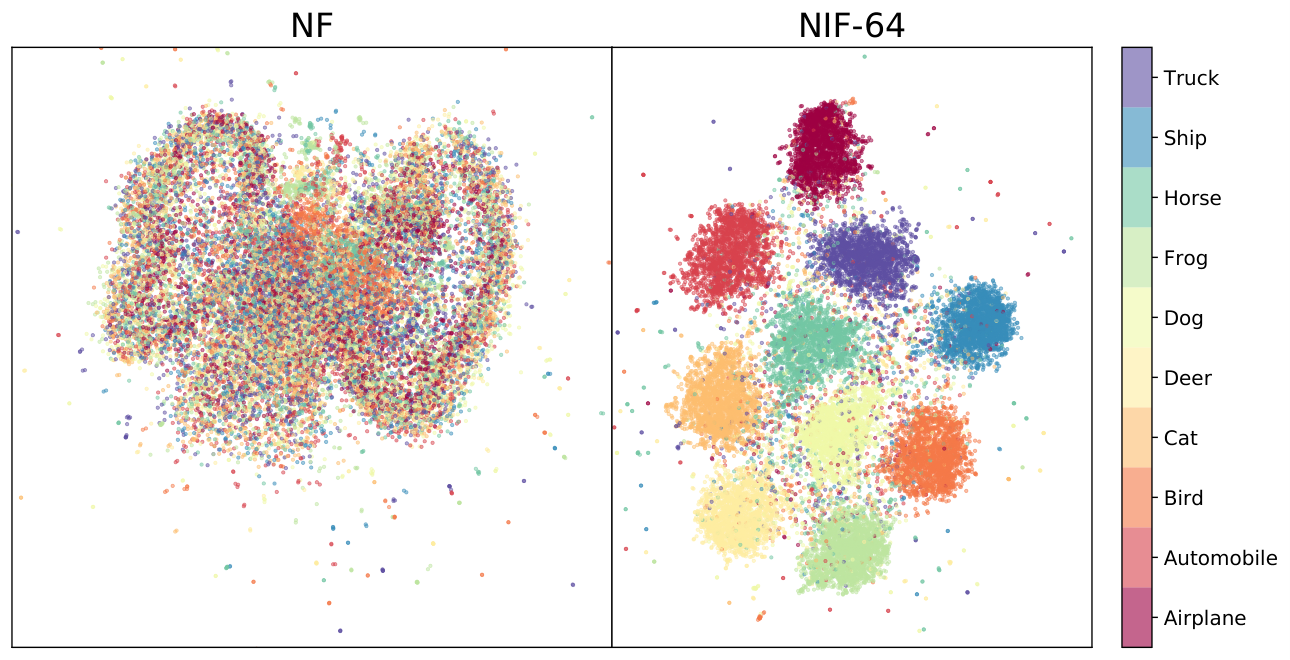
Noisy injective flows also provide embeddings of the data that are more easily separable. We use supervised UMAP [23] to produce a low-dimensional embedding of the CIFAR-10 [20] test set. Fig. 4 shows that the NIF embedding cleanly separates the data from different classes while the NF embeddings cannot.


5.2 Controlling deviations from the manifold
We show that a single scalar parameter introduced at test time can provide a simple method to control deviations from the manifold. The test time scalar parameter, , controls the variance of a Gaussian NIF layer: . There are two notable settings of : leaves the model unchanged while corresponds to the injective flow defined over the learned manifold .
Samples from our model when are generated directly on our learned manifold . In Fig. 5, we compare samples from the CelebA dataset [22] from the baseline normalizing flow and from our method with . The samples generated on the manifold of the NIF are clearer and exhibit more cohesive facial structure than the samples from the normalizing flow. Samples from the manifold exhibit the high level features that our model has learned. In the appendix we provide more samples from the manifold of models learned for Fashion MNIST and CIFAR-10.
We observe that increasing for a given point on the manifold will increase the amount of noise the sample exhibits. Fig. 6 shows the effect of a sample as it is moved away from the manifold. Visually it may seem like deviating from the manifold serves no purpose other than adding random noise, however we find that small deviations from the manifold may add imperceptible features to the image. We find evidence of this in how the FID varies with .
Fréchet Inception Distance (FID) [12] is a quantity used to measure the sample performance of a generative model. It computes a distance between two probability distributions by comparing the distributions of the activations of a state-of-the-art classifier for the Image-Net [8] dataset on samples from each dataset. While FID has been shown to correlate with visual quality, at its core it can measure features that the classifier has learned. Fig. 7 shows that for some non-zero value of , the resulting NIF can yield significantly better FID values. Given that non-zero values of do not correspond to clear visual changes in images, we can interpret the result of Fig. 7 to mean that slight deviations from the learned manifold correspond to noise in a feature space that is perceptible to a classifier. By tuning over a random sub-sample of the training set and computing FID over a test set, noisy injective flows are able to either match or significantly outperform normalizing flows in FID, as shown in Tab. 2. In the appendix we investigate this phenomenon farther on the CIFAR-10 dataset [20].
At , we can evaluate if the latent dimensionality has a detrimental effect on log-likelihood. We see in table 2 that this is not the case as noisy injective flows perform similar to or slightly better than normalizing flows in bits per dim across many latent state sizes and datasets.
| Model | Fashion MNIST | CIFAR-10 | CelebA |
| NF | 42.77 | 78.58 | 63.07 |
| NIF-64 | 23.97 | 80.15 | 30.96 |
| NIF-128 | 23.23 | 79.38 | 34.46 |
| NIF-256 | 24.84 | 78.44 | 33.95 |
| NIF-512 | 25.34 | 77.47 | 35.96 |
| Model | Fashion MNIST | CIFAR-10 | CelebA |
| NF | 1.518 | 1.072 | 0.852 |
| NIF-64 | 1.506 | 1.069 | 0.839 |
| NIF-128 | 1.506 | 1.071 | 0.835 |
| NIF-256 | 1.515 | 1.073 | 0.830 |
| NIF-512 | 1.523 | 1.070 | 0.838 |
6 Conclusion
We have presented a new probabilistic model, noisy injective flows, that generalizes normalizing flows. The use of a stochastic inverse allows the method to transform across dimensions while maintaining the strengths of normalizing flows. We have presented an instance of NIFs that can be used to enhance existing flow models. We have demonstrated that our method was able to learn representations of data that are both low-dimensional and better than those learned by NFs. We also show that our model can be tuned to generate widely varied, high quality images, based on CelebA and Fashion MNIST. Noisy injective flows serve to bridge the gap between normalizing flows and state-of-the-art image generating methods while retaining the advantages of normalizing flows.
References
- Au and Tam [1999] Chi Au and Judy Tam. Transforming Variables Using the Dirac Generalized Function. The American Statistician, 53:270–272, 1999.
- Boothby [1975] W. Boothby. An Introduction to Differentiable Manifolds and Riemannian Geometry, volume 63 of Pure and Applied Mathematics. Elsevier, 1975. ISBN 978-0-12-116050-0. doi: 10.1016/S0079-8169(08)X6065-9. URL https://linkinghub.elsevier.com/retrieve/pii/S0079816908X60659.
- Bradbury et al. [2018] James Bradbury, Roy Frostig, Peter Hawkins, Matthew James Johnson, Chris Leary, Dougal Maclaurin, and Skye Wanderman-Milne. JAX: composable transformations of Python+NumPy programs, 2018. URL http://github.com/google/jax.
- Brehmen and Cranmer [2020] Johann Brehmen and Kyle Cranmer. Flows for simultaneous manifold learning and density estimation. April 2020. URL https://arxiv.org/pdf/2003.13913.pdf.
- Casella and Berger [2002] G. Casella and R.L. Berger. Statistical Inference. Duxbury advanced series in statistics and decision sciences. Thomson Learning, 2002. ISBN 978-0-534-24312-8. URL https://books.google.com/books?id=0x_vAAAAMAAJ.
- Chen et al. [2019] Tian Qi Chen, Jens Behrmann, David Duvenaud, and Jörn-Henrik Jacobsen. Residual flows for invertible generative modeling. In Hanna M. Wallach, Hugo Larochelle, Alina Beygelzimer, Florence d’Alché-Buc, Emily B. Fox, and Roman Garnett, editors, Advances in Neural Information Processing Systems 32: Annual Conference on Neural Information Processing Systems 2019, NeurIPS 2019, 8-14 December 2019, Vancouver, BC, Canada, pages 9913–9923, 2019. URL http://papers.nips.cc/paper/9183-residual-flows-for-invertible-generative-modeling.
- Dai and Wipf [2019] Bin Dai and David P. Wipf. Diagnosing and enhancing VAE models. In 7th International Conference on Learning Representations, ICLR 2019, New Orleans, LA, USA, May 6-9, 2019. OpenReview.net, 2019. URL https://openreview.net/forum?id=B1e0X3C9tQ.
- Deng et al. [2009] J. Deng, W. Dong, R. Socher, L.-J. Li, K. Li, and L. Fei-Fei. ImageNet: A Large-Scale Hierarchical Image Database. In CVPR09, 2009.
- Dinh et al. [2017] Laurent Dinh, Jascha Sohl-Dickstein, and Samy Bengio. Density estimation using real NVP. In 5th International Conference on Learning Representations, ICLR 2017, Toulon, France, April 24-26, 2017, Conference Track Proceedings. OpenReview.net, 2017. URL https://openreview.net/forum?id=HkpbnH9lx.
- Fefferman et al. [2013] Charles Fefferman, Sanjoy Mitter, and Hariharan Narayanan. Testing the Manifold Hypothesis. arXiv:1310.0425 [math, stat], December 2013. URL http://arxiv.org/abs/1310.0425.
- Gemici et al. [2016] Mevlana C. Gemici, Danilo Rezende, and Shakir Mohamed. Normalizing Flows on Riemannian Manifolds. arXiv:1611.02304 [cs, math, stat], November 2016. URL http://arxiv.org/abs/1611.02304.
- Heusel et al. [2017] Martin Heusel, Hubert Ramsauer, Thomas Unterthiner, Bernhard Nessler, and Sepp Hochreiter. Gans trained by a two time-scale update rule converge to a local nash equilibrium. In Isabelle Guyon, Ulrike von Luxburg, Samy Bengio, Hanna M. Wallach, Rob Fergus, S. V. N. Vishwanathan, and Roman Garnett, editors, Advances in Neural Information Processing Systems 30: Annual Conference on Neural Information Processing Systems 2017, 4-9 December 2017, Long Beach, CA, USA, pages 6626–6637, 2017. URL http://papers.nips.cc/paper/7240-gans-trained-by-a-two-time-scale-update-rule-converge-to-a-local-nash-equilibrium.
- Ho et al. [2019] Jonathan Ho, Xi Chen, Aravind Srinivas, Yan Duan, and Pieter Abbeel. Flow++: Improving flow-based generative models with variational dequantization and architecture design. In Kamalika Chaudhuri and Ruslan Salakhutdinov, editors, Proceedings of the 36th International Conference on Machine Learning, ICML 2019, 9-15 June 2019, Long Beach, California, USA, volume 97 of Proceedings of Machine Learning Research, pages 2722–2730. PMLR, 2019. URL http://proceedings.mlr.press/v97/ho19a.html.
- Hoffman et al. [2013] Matthew D. Hoffman, David M. Blei, Chong Wang, and John W. Paisley. Stochastic variational inference. J. Mach. Learn. Res., 14(1):1303–1347, 2013. URL http://dl.acm.org/citation.cfm?id=2502622.
- Jordan et al. [1998] Michael I. Jordan, Zoubin Ghahramani, Tommi S. Jaakkola, and Lawrence K. Saul. An Introduction to Variational Methods for Graphical Models. In Michael I. Jordan, editor, Learning in Graphical Models. Springer Netherlands, Dordrecht, 1998. ISBN 978-94-010-6104-9 978-94-011-5014-9. doi: 10.1007/978-94-011-5014-9_5. URL http://link.springer.com/10.1007/978-94-011-5014-9_5.
- Karras et al. [2018] Tero Karras, Timo Aila, Samuli Laine, and Jaakko Lehtinen. Progressive growing of gans for improved quality, stability, and variation. In 6th International Conference on Learning Representations, ICLR 2018, Vancouver, BC, Canada, April 30 - May 3, 2018, Conference Track Proceedings. OpenReview.net, 2018. URL https://openreview.net/forum?id=Hk99zCeAb.
- Karras et al. [2020] Tero Karras, Samuli Laine, Miika Aittala, Janne Hellsten, Jaakko Lehtinen, and Timo Aila. Analyzing and Improving the Image Quality of StyleGAN. arXiv:1912.04958 [cs, eess, stat], March 2020. URL http://arxiv.org/abs/1912.04958.
- Kingma and Dhariwal [2018] Diederik P. Kingma and Prafulla Dhariwal. Glow: Generative flow with invertible 1x1 convolutions. In Samy Bengio, Hanna M. Wallach, Hugo Larochelle, Kristen Grauman, Nicolò Cesa-Bianchi, and Roman Garnett, editors, Advances in Neural Information Processing Systems 31: Annual Conference on Neural Information Processing Systems 2018, NeurIPS 2018, 3-8 December 2018, Montréal, Canada, pages 10236–10245, 2018. URL http://papers.nips.cc/paper/8224-glow-generative-flow-with-invertible-1x1-convolutions.
- Kingma and Welling [2014] Diederik P. Kingma and Max Welling. Auto-encoding variational bayes. In Yoshua Bengio and Yann LeCun, editors, 2nd International Conference on Learning Representations, ICLR 2014, Banff, AB, Canada, April 14-16, 2014, Conference Track Proceedings, 2014. URL http://arxiv.org/abs/1312.6114.
- [20] Alex Krizhevsky. Learning Multiple Layers of Features from Tiny Images. page 60.
- Kumar et al. [2020] Abhishek Kumar, Ben Poole, and Kevin Murphy. Regularized Autoencoders via Relaxed Injective Probability Flow. In AISTATS, 2020.
- Liu et al. [2015] Ziwei Liu, Ping Luo, Xiaogang Wang, and Xiaoou Tang. Deep learning face attributes in the wild. In Proceedings of International Conference on Computer Vision (ICCV), December 2015.
- McInnes et al. [2018] Leland McInnes, John Healy, Nathaniel Saul, and Lukas Grossberger. Umap: Uniform manifold approximation and projection. The Journal of Open Source Software, 3(29):861, 2018.
- Papamakarios et al. [2019] George Papamakarios, Eric Nalisnick, Danilo Jimenez Rezende, Shakir Mohamed, and Balaji Lakshminarayanan. Normalizing Flows for Probabilistic Modeling and Inference. arXiv:1912.02762 [cs, stat], December 2019. URL http://arxiv.org/abs/1912.02762.
- Ratliff [2014] Nathan Ratliff. Multivariate Calculus II: The geometry of smooth maps, 2014. URL https://ipvs.informatik.uni-stuttgart.de/mlr/wp-content/uploads/2014/12/mathematics_for_intelligent_systems_lecture6_notes.pdf.
- Razavi et al. [2019] Ali Razavi, Aäron van den Oord, and Oriol Vinyals. Generating diverse high-fidelity images with VQ-VAE-2. In Hanna M. Wallach, Hugo Larochelle, Alina Beygelzimer, Florence d’Alché-Buc, Emily B. Fox, and Roman Garnett, editors, Advances in Neural Information Processing Systems 32: Annual Conference on Neural Information Processing Systems 2019, NeurIPS 2019, 8-14 December 2019, Vancouver, BC, Canada, pages 14837–14847, 2019. URL http://papers.nips.cc/paper/9625-generating-diverse-high-fidelity-images-with-vq-vae-2.
- Rezende and Mohamed [2015] Danilo Jimenez Rezende and Shakir Mohamed. Variational inference with normalizing flows. In Francis R. Bach and David M. Blei, editors, Proceedings of the 32nd International Conference on Machine Learning, ICML 2015, Lille, France, 6-11 July 2015, volume 37 of JMLR Workshop and Conference Proceedings, pages 1530–1538. JMLR.org, 2015. URL http://proceedings.mlr.press/v37/rezende15.html.
- Song and Ermon [2019] Yang Song and Stefano Ermon. Generative modeling by estimating gradients of the data distribution. In Hanna M. Wallach, Hugo Larochelle, Alina Beygelzimer, Florence d’Alché-Buc, Emily B. Fox, and Roman Garnett, editors, Advances in Neural Information Processing Systems 32: Annual Conference on Neural Information Processing Systems 2019, NeurIPS 2019, 8-14 December 2019, Vancouver, BC, Canada, pages 11895–11907, 2019. URL http://papers.nips.cc/paper/9361-generative-modeling-by-estimating-gradients-of-the-data-distribution.
Appendix A Derivations
A.1 Notation
A.2 Equation 1 - Change of variable formula
| (14) | ||||
| (15) | ||||
| (16) | ||||
| (17) | ||||
| (18) |
This general change of variable equation describes the probability density function of a transformed random variable. When is invertible and , we can recover the standard normalizing flows change of variable formula.
A.3 Equation 6 - Noisy injective flows marginal distribution
| (19) | |||
| (20) | |||
| (21) | |||
| (22) | |||
| we use the sifting property of the delta function to evaluate the integral | |||
| (23) |
In section 3.2 we showed that the convolved pdf is the marginal distribution over when the joint is defined as . However there is a more interpretable form of this equation that follows by letting :
| (24) |
This resulting equation has an intuitive explanation - the pdf of noisy injective flows is defined as the expected value, over the noise model constrained to the learned manifold, of the injective change of variable formula from Eq. (5). Although this form has no practical use, it serves to further justify the construction of noisy injective flows.
A.4 Proposition 1 - Modes of the stochastic inverse are pseudo inverses
The modes of are at the values of that maximize . If we assume that , we have:
| (25) | |||
| (26) | |||
| (27) | |||
| (28) | |||
| (29) | |||
| (30) | |||
| (31) | |||
| (32) |
A.5 Equation 10 - Evidence lower bound
| (33) | |||
| (34) | |||
| (35) | |||
| (36) |
A.6 Equation 12 - Gaussian NIF
| (37) | ||||
| (38) | ||||
| (39) | ||||
| (40) | ||||
| (41) | ||||
| (42) | ||||
| (43) |
We use the names and because the values they represent are the log partition functions of and respectively.
A.7 Equation 13 - Closed form Gaussian NIF
We start by proving the identity:
| (44) |
Proof: Consider a Gaussian probability density function: . Because probability density functions integrate to 1, we have
| (45) | |||
| (46) | |||
| (47) | |||
| (48) |
With this identity, we can proceed with the main derivation:
| (49) | |||
| (50) | |||
| (51) | |||
| (52) | |||
| (53) | |||
| (54) | |||
| We use the identity from above to introduce | |||
| (55) | |||
| (56) | |||
| (57) |
Eq. (57) yields a simple equation that can be used to compute , however to embed an in the latent space, we use the pseudo-inverse of on the hyperplane, which takes the form:
| (58) |
Appendix B Additional Plots
B.1 Fashion MNIST

B.2 CelebA Reconstructions


B.3 CIFAR-10 Results
Noisy injective flows have a difficult time learning datasets that likely do not satisfy the manifold hypothesis such as CIFAR-10, however noisy injective flows can revert to the generative performance of normalizing flows by sampling off of the manifold. Figure 10 shows samples from the baseline normalizing flow and noisy injective flow (with latent dimension of 128) from the experiments section. The plot in the middle shows, figure 10(b) samples from the manifold of the NIF. The sample lack features of images that one expect to be present in CIFAR images. However, when we sample from off the manifold () like in figure 10(c), noisy injective flows produce samples that resemble those from the normalizing flow.The plot of FID vs s in figure 11 provides a similar result. The FID score of the NIF is poor when sampling on the manifold, but reverts back to that of the baseline normalizing flow as is increased to 1.
B.4 Deep noisy injective flow
Here we show samples from a noisy injective flow whose architecture resembles figure 2. This model used a latent state size of 128, used a low dimensional normalizing flow that consisted of 10 affine coupling layers, each with a 4 layer MLP with 1024 units in each hidden layer, and act norm and reverse layers in between each affine coupling. A standard Gaussian NIF from section 4 was used to change dimension into the same GLOW architecture described in the experiments section, but with 512 channels in each convolutional filter.
The use of a low dimensional normalizing flow allows the model to learn a probability density over the manifold. Then the high dimensional flow is able to shape the manifold to fit data. As a result, we see more variation in the images produced by this kind of noisy injective flow, especially at higher temperatures.
This model produced figure 1. We found that it produced the best samples at higher temperatures ( was used in figure 1). Below we show samples from this model at varying temperatures.


