Equilibrium current vortices in rare-earth–doped simple metals

The conversion of spin currents into excitations of the charge, phonon, photon, or magnetization degrees of freedom and vice versa OtaniSpinConv often involves spin-orbit interactions (SOI) SOT2013. Examples are the spin-orbit torques Daichi2015, charge pumping ChargePumping2015, magnetoelastic interactions PhononMaekawa, and electric-field-induced magnetization dynamics Elec1; Elec2. The large intraatomic SOI that governs the local moments of lanthanides with partially filled 4f subshells causes novel spin charge coupling voltage and affects device parameters such as the magnetic damping REDoping; RECapping. Rare-earth (RE) ions with local magnetic moments can partially or entirely substitute the non-magnetic yttrium in the ferrimagnetic insulator yttrium iron garnet Y₃Fe₅O₁₂ (YIG) YIG. The different magnetic sublattices of RE-IG strongly modify the magnetic properties RIG1; RIG2; RIG3, causing, for example, different compensation points for the magnetic and total angular moments DoubleCompensation. A more complex phenomenon is a double sign change of the spin Seebeck effect GIG. Thulium iron garnet (Tm₃Fe₅O₁₂) films with perpendicular magnetization Kubota2012; Tang2016; TIG2018 can be switched by current-induced spin-orbit torques TmIG0; TmIG1; TmIG2.

These new developments come on top of decades of research on 4f electrons in bulk metals BookJensen. For example, RE impurities in non-magnetic metals cause an anomalous Hall effect at low doping concentrations Fert. The magnetization in rare-earth intermetallics originates from both the 5d and 6s conduction electrons and 4f moments (see Ref. REIntermetallics and references therein). The hybridization of RE moments with conduction electrons affects the susceptibility in rare-earth dialuminides, REAl₂ REAl2, or causes enhanced magnetic moments of RE dopants in Ag and Au Devine.

In topological superconductors, such as the Fe(Te, Se), a vortex with a Friedel-like oscillatory profile around magnetic impurities has been reported SCVortex.

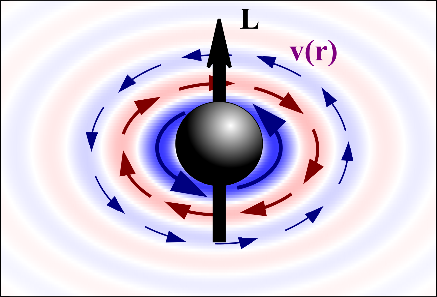
Here we present a theoretical study of the coupling of a 4f local moment with the Fermi sea of a simple metal host. We predict a charge current circling the impurity with a direction that oscillates radially, as illustrated in Fig. 1. Our starting point for the interaction between the local 4f moments and the conduction electrons is the Kondo Hamiltonian Kondo. Its chirality induces a circulating current whose vorticity is governed by the direction of the RE orbital moment and generates an Ørsted magnetic field. The induced radial current distribution oscillates with the same period as the RKKY spin polarization RKKY and for the same physical reason, i.e., the finite momentum cut-off at the Fermi surface. The predicted trends should be observable in principle by NMR or scanning microscopy. The present study of the interaction between conduction electrons and 4f magnetic moments contributes to understanding spintronic devices including rare-earth local moments, such as interfaces between rare-earth iron garnets and nonmagnetic metals.

Rare-earth atoms generally appear in materials as triply charged cations. Their partially filled 4f subshell governs their magnetic properties. The 4f electrons only weakly interact with their environment Liu1961; BookJensen due to their small orbital radius and shielding by the more extended and fully occupied $5s$ and $5p$ orbitals. This does not exclude a significant exchange interaction: the conduction electrons of Pt contacts activate the Gd moments in gadolinium gallium garnet (GGG) OyanagiGGG. The exchange interaction between a local spin with conduction electrons of a metal host generates RKKY spin-density oscillations. Triply charged Lanthanide anions have electronic configuration [Xe] 4fⁿ, where the number of 4f electrons $n$ goes from $n=0$ for La⁺³ to $n=14$ for Lu⁺³. Except for $n=0$ (La⁺³), $n=7$ (Gd⁺³), and $n=14$ (Lu⁺³), the intra-atomic spin-orbit interaction critically affects the magnetic properties. Here we address a spin-orbit proximity effect of such a magnetic moment embedded in a Fermi sea.

A partially occupied 4f subshell is characterized by a spin $\mathbf{S}$, an orbital moment $\mathbf{L}$, and a total angular moment $\mathbf{J}=\mathbf{L}+\mathbf{S}$ Sievers; BookJensen. For the basis $|\Psi\rangle\equiv|{S,L,J,J_{z}}\rangle$, $\mathbf{S}^{2}|\Psi\rangle=\hbar^{2}S(S+1)|\Psi\rangle$, $\mathbf{L}^{2}|\Psi\rangle=\hbar^{2}L(L+1)|\Psi\rangle$, $\mathbf{J}^{2}|\Psi\rangle=\hbar^{2}J(J+1)|\Psi\rangle$, $\hat{J_{z}}|\Psi\rangle=\hbar J_{z}|\Psi\rangle$, where $\hbar$ is the reduced Planck constant. Hund’s rules specify the quantum numbers $S$, $L$, and $J$ of the ground state manifold, while $J_{z}$ depends on the applied magnetic and electric fields. Within a manifold of constant $S$, $L$, and $J$, the Wigner-Eckart theorem ensures collinearity of all angular moment vectors: $\mathbf{S}=(g_{J}-1)\mathbf{J}$, $\mathbf{L}=(2-g_{J})\mathbf{J}$, and $\mathbf{L}+2\mathbf{S}=g_{J}\mathbf{J}$, where $g_{J}=3/2+[S(S+1)-L(L+1)]/[2J(J+1)]$ is the Landé g-factor.

We model the system as a single RE local moment embedded into a free electron gas, which is appropriate for most dilute alloys. Conduction electrons interact with the rare-earth spin and orbital moment via the Kondo Hamiltonian Kondo. Here, we address equilibrium properties that are affected by the spin-independent skew scattering but disregard external current-induced phenomena such as the spin-Hall effect. We operate in a regime above the Kondo temperature, and treat $\mathbf{J,S}$ and $\mathbf{L}$ as classical vectors. The strongly localized 4f orbital radius governs the spatial extent of the coupling. When the 4f orbital radius is much smaller than the typical wavelength of the conduction electrons, the moment couples to free electrons by a contact interaction.

The $s$-$f$ exchange interaction in the Kondo Hamiltonian is similar to the $s$-$d$ Hamiltonian for $3d$-transition-metals Liu1961; SFInteraction1; SFInteraction2; Kondo. It reads

where $\boldsymbol{\sigma}$ is the vector of Pauli matrices and $\delta^{\mathrm{4f}}\left(\mathbf{r}\right)$ is a Dirac delta representing the localized 4f subshell. In a free electron gas with Fermi wave number $k_{F}$, the exchange constant Kondo is $J_{ex}=2e^{2}A_{3}(0)/(7\epsilon_{0}k_{F}^{2})$, where the radial integral Kondo $A_{h}(n)=\int_{0}^{\infty}dx_{1}x_{1}^{2}\int_{0}^{\infty}dx_{2}x_{2}^{2}j_{n}(x_{1})j_{n}(x_{2})x_{<}^{h}/x_{>}^{h+1}R(r_{1})R(r_{2})$, with $x_{1}=k_{F}r_{1}$, $x_{2}=k_{F}r_{2}$, $x_{<}=\min(x_{1},x_{2})$, and $x_{>}=\max(x_{1},x_{2})$. $A_{h}(n)$ can be evaluated numerically using a Slater-type orbital for the radial part of the 4f wave function $R(r)\sim r^{3}e^{-r/a}$ normalized over a large volume, $\int_{0}^{\infty}drr^{2}R^{2}(r)=1$. The constant $a$ is related to the 4f radius by $\langle r\rangle=\int_{0}^{\infty}drr^{3}R^{2}(r)=9a/2$. With $k_{F}=1.75$ Å^-1 for Al and $\langle r\rangle=0.6$ Å BookJensen, $A_{3}(0)=0.33$ and $J_{ex}=5.6$ eV ų.

The so-called spin-independent skew scattering affects the trajectories of the electron charge and is responsible for the anomalous Hall effect in metals with RE impurities Fert; Kondo; Giovannini. As shown below, it also affects the ground state. Its Hamiltonian reads Kondo

where $\mathbb{I}_{2\times 2}$ is the identity matrix in Pauli spin space, and $\eta\left(\mathbf{r}\right)=\eta_{0}\delta^{\mathrm{4f}}\left(\mathbf{r}\right)$ with $\eta_{0}=9e^{2}\left[A_{2}(1)-(5/9)A_{4}(1)\right]\left(140\epsilon_{0}\hbar k_{F}^{4}\right)^{-1}$. For the parameters introduced above, $A_{2}(1)\sim 0.0885$, $A_{4}(1)=0.056$, and $\hbar\eta_{0}k_{F}^{2}=0.21$ eV ų. Both exchange and skew-scattering interactions are active in a volume $V_{\mathrm{4f}}\lesssim 10\,\mathrm{\mathring{A}}^{3}$. The energy scales $\langle H_{\mathrm{skew}}\rangle\sim\hbar\eta_{0}k_{F}^{2}/V_{\mathrm{4f}}=\mathcal{O}\left(10\,\mathrm{meV}\right)$ and $\langle H_{sf}\rangle\sim J_{ex}/V_{\mathrm{4f}}=\mathcal{O}\left(100\,\mathrm{meV}\right)$ are consistent with published values extracted from experiments, such as the Knight shift StrengthSF, electron spin resonance RettoriStrengthSF, and magnetoresistance FertStrengthSF; FertAndLevyStrengthSF; GiovaniStrengthSF. $H_{\mathrm{skew}}$ deflects free electrons via an effective local force caused by the 4f subshell with orbital angular momentum $\mathbf{L}$. Equation (2) does not contain an explicit SOI parameter because we operate in the limit of large 4f spin-orbit interaction that generates a finite $\left|\mathbf{L}\right|$.

The 4f RE impurities in noble metals hybridize with 5d virtual-bound states of the conduction electrons GeneralModelForImpurities, which can be parameterized in terms of phase shifts of angular momentum scattering channels FertStrengthSF. The enhancement of the magnetic moments of pure RE metals ExcessInPureMetals1; ExcessInPureMetals2; ExcessInPureMetals3 and in RE-doped Ag and Au Devine; Bak has been attributed to those 5d virtual bound states. Here we focus on the spin and orbital polarization induced by the Kondo Hamiltonian on conduction electrons that we describe by plane waves without truncating an expansion into spherical harmonics. To leading order in the contact interaction, we may discard hybridization and orthogonalization corrections.

Next, we discuss the RKKY spin polarization due to the $H_{sf}$ and the response induced by $H_{\mathrm{skew}}$. We focus on ions with partially filled 4f shells. Gd³⁺ ($L=0$) can create an RKKY spin polarization, but its $H_{\mathrm{skew}}$ vanishes. We do not address Eu³⁺ since its spin and orbital moment cancel in its ground ($J=0$) but not in excited states.

In the mean-field, local-density approximation, Eq. (1) for an RE moment at the origin $\mathbf{r}=0$ becomes

where $\mathbf{s}(\mathbf{r})\equiv\left\langle\Psi_{c}^{\dagger}(\mathbf{r})\left|\hbar\boldsymbol{\sigma}/2\right|\Psi_{c}(\mathbf{r})\right\rangle$ is the spin density of the conduction-electron wave function $\Psi_{c}$. For a static moment and to leading order in $J_{ex}$, we recover the RKKY spin density oscillations

where $\chi(r)$ is the susceptibility and $D_{e}=m_{e}k_{F}(\pi\hbar)^{-2}$ the density of states of the host metal at the Fermi energy. Figure 2(a) illustrates the characteristic RKKY oscillations in $r\chi(r)$ that contribute to the total spin magnetic moment $\mathbf{m}_{S}$

where the bare $g$-factor is $g_{S}=2$, $\gamma_{0}=e/(2m_{e})$ is the modulus of the gyromagnetic ratio, $-e$ is the electron charge, and the constant $G_{i}^{S}=J_{ex}D_{e}/4$. For example, in Al, $G_{i}^{S}\approx 0.13.$ The polarization cloud enhances the total spin magnetic moment and $g$-factor by $G_{i}^{S}$, which can be observed via the imaginary part of the spin-mixing conductance (effective field) at ferromagnet$|$normal metal interfaces crystalfield or spin-dependent interfacial phase shifts at ferromagnet$|$ superconductor interfaces Cottet.

We now show that the Kondo Hamiltonian generates equilibrium charge-current vortices around the impurity. In Fourier representation with linear momentum $\hbar\mathbf{q}$ and unperturbed wave function $\langle\mathbf{r}|\mathbf{q}\rangle=e^{i\mathbf{r}\cdot\mathbf{q}}/\sqrt{\Omega}$, the matrix elements of the skew-type interaction read

where $e^{-2k^{2}a^{2}}$ cuts off an ultraviolet divergence of a delta-function potential. To leading order in $\eta_{0}$, we find a spin-independent velocity field of conduction electrons (see Appendix A):

where

and $x=k_{F}r$. In the delta-function $a\rightarrow 0,$ the response function $f$ should used in Equation (8) instead of $F$. Outside the 4f subshell, $F$ and $f$ are similar, see Fig. 2(b). $F$, $f$, and $\chi$ oscillate with wavenumber $2k_{F}$ and are approximated by $\cos\left(2k_{F}r\right)/r^{3}$ far from the atom. The integrated modulus of the velocity,

is of the order of a percent of the Fermi velocity $v_{F}=\hbar k_{F}/m_{e}\sim 2\times 10^{6}$ m/s and $\bar{v}_{s}\sim 10$ km/s for Al.

The radial density of the orbital angular momentum

is at equilibrium always collinear with $\mathbf{L}$ and parallel to it near the origin. Both the orbital density of the rotational current and the RKKY spin polarization decay algebraically and oscillate with increasing distance from the origin [see Fig. 2(b)]. Therefore, the current response has paramagnetic as well as diamagnetic contributions. Note that the spin and orbital radial distributions have a phase difference for small radius, as shown in Fig. 2.

The orbital magnetic moment is dressed by the electron gas

where the bare orbital $g$-factor $g_{L}=1$, and $G_{i}^{L}=2m_{e}\eta_{0}k_{F}^{3}/\left(3\pi^{2}\hbar\right)$, or

where $n_{\mathrm{4f}}=V_{\mathrm{4f}}n_{0}$ is the number of conduction electrons in the volume of the 4f subshell, $V_{\mathrm{4f}}\sim 10$ Å³, with $n_{0}=k_{F}^{3}/\left(3\pi^{2}\right)$ the metal density. The energy of orbital-orbital coupling is $E_{\eta}=\hbar\eta_{0}k_{F}^{2}/V_{\mathrm{4f}}$, while the host Fermi energy is $E_{F}=\hbar^{2}k_{F}^{2}/\left(2m_{e}\right)$. Thus, the strength of the rotational current momentum, with respect to $\mathbf{L}$, is proportional to the ratio of the orbital coupling and Fermi energies. The proportionality constant is the average number of conduction electrons subject to the coupling potential. For the present parameters we find $n_{\mathrm{4f}}\approx 1.8$, $E_{\eta}\approx 0.02$ eV, $E_{F}=11.7$ eV, and a relatively small value $G_{i}^{L}\approx 1/300$.

The current vortex induces an Ørsted field

where $\mu_{0}=4\pi\times 10^{-7}$ $\mathrm{J}/\left(\mathrm{mA}^{2}\right)$ is the magnetic permeability of free space. The velocity and magnetic fields are proportional to the RE orbital momentum, $|\left\langle\mathbf{v}\right\rangle|\propto|\mathbf{B}_{\mathrm{\O}}|\propto\eta_{0}|\mathbf{L}|$. Far from the RE ion, $R\gg\langle r\rangle$,

is the field generated by the magnetic dipole $\mathbf{m_{\mathrm{rc}}}=-\gamma_{0}G_{i}^{L}\mathbf{L}$. $\mathbf{B}_{\mathrm{\O}}$ is proportional to the dipolar magnetic field by the 4f orbital momentum ($\mathbf{B}_{\mathbf{L}}$), i.e., $\mathbf{B}_{\mathrm{\O}}=G_{i}^{L}\mathbf{B}_{\mathbf{L}}$, with $G_{i}^{L}\ll 1$.

At the origin and for $k_{F}=1.75$/Å

Figure 3 shows the $z$-component of this field as a function of distance $\mathbf{r}=x\mathbf{e_{x}}$, where the unit vectors $\mathbf{e_{x}}$ and $\mathbf{e_{z}}$ pointing along the $x$- and $z$-Cartesian axis, respectively. The field is negative close to the origin but turns positive and decays to zero in an oscillatory fashion.

The field at the origin, $\mathbf{B}_{\text{{\O}}}(\mathbf{0})$, couples to the local nuclear spin by the Zeeman interaction, that shifts the nuclear magnetic resonance (NMR) frequency by $\Delta\omega=\gamma_{N}\left|\mathbf{B}_{\text{{\O}}}(\mathbf{0})\right|\sim 5$ MHz, where $\gamma_{N}$ is the nuclear gyromagnetic ratio. In an NMR experiments, a constant magnetic field $B_{0}\mathbf{e_{z}}$ polarizes the nuclear moments as well as the 4f moments along the $z$-direction. The Knight shift $K$ produced by the current and parameterized by the ratio of the internal and applied magnetic fields SolidBookKittel, at low temperatures ($T\lesssim 1$ K) is

where we assume full polarization of the magnetic moment of the 4f subshell. The nuclear magnetic resonance frequency is typically in the 100 MHz regime for applied (constant) fields of $B_{0}\sim 10$ T. For a given rf frequency we therefore predict different resonance magnetic fields for rare earth impurities in an insulating and metallic host. We hope that our results stimulate experiments that can identify the ground state current vortices.

Orbital contributions to the Knight shift have been predicted before Devine; KnightShiftInSystemsWithSOC, holding virtual bound states of conduction electrons at RE impurities in a metal host responsible Devine. These theories are not compatible with our model since they predict effects for half-filled shells without orbital moment (Gd).

We predict that RE local moments interact with the conduction electrons of a metallic host to generate both an oscillating spin density and charge current, the latter by the spin-independent skew-scattering interaction. The radial distribution of the induced velocity field oscillates with the same period as the RKKY spin polarization induced by the local exchange interaction. A finite 4f orbital moment $\mathbf{L}$ is necessary to form the current in the electron gas. Therefore, the predicted magnetic field and Knight shift depend linearly with $\left|\mathbf{L}\right|\propto\left(2-g_{J}\right)\left|\mathbf{J}\right|$ and vanish for RE-doped insulators. Furthermore, the induced magnetic field depends on the atomic number via the Landé g-factor ground-state quantum numbers. Several approximations are crude, but we are confident about the predicted trends. Relativistic first-principles calculations of open 4f subshells in a metal host should improve the accuracy of the predictions.

The Ørsted fields generated by RE impurities at the surface of a metal with sufficiently large Fermi wavelength can be measured in principle by scanning magnetometries based on nano-scale superconducting quantum interference devices (nanoSQUID) NanoSquid2 or optically read-out nitrogen-vacancy (NV)-centers NVCenters1; NVCenters2. RE impurities adsorbed at a surface 2D electron gas, or graphene monolayer are promising candidate systems to image the predicted equilibrium current vortices.

We thank Jiang Xiao and Koichi Oyanagi for fruitful discussions. This research was supported by JSPS KAKENHI Grant No. 19H006450, Postdoctorado FONDECYT 2019 Folio 3190030, and PUTIQ1 Grant of Universitas Indonesia NKB-1369/UN2.RST/HKP.05.00/2020.

References

• (1) Y. Otani, M. Shiraishi, A. Oiwa, E. Saitoh, and S. Murakami, Spin conversion on the nanoscale, Nat. Phys. 13, 829 (2017).
• (2) K. Garello, I. M. Miron, C. O. Avci, F. Freimuth, Y. Mokrousov, S. Blügel, S. Auffret, O. Boulle, G. Gaudin, and P. Gambardella, Symmetry and magnitude of spin-orbit torques in ferromagnetic heterostructures, Nat. Nano. 8, 587 (2013).
• (3) K. Nomura and D. Kurebayashi, Charge-Induced Spin Torque in Anomalous Hall Ferromagnets, Phys. Rev. Lett. 115, 127201 (2015).
• (4) C. Ciccarelli, K. M. D. Hals, A. Irvine, V. Novak, Y. Tserkovnyak, H. Kurebayashi, A. Brataas, and A. Ferguson, Magnonic charge pumping via spin-orbit coupling, Nat. Nano. 10, 50 (2015).
• (5) M. Mori, A. Spencer-Smith, O. P. Sushkov, and S. Maekawa, Origin of the Phonon Hall Effect in Rare-Earth Garnets, Phys. Rev. Lett. 113, 265901 (2014).
• (6) A. M. Kadomtseva, Y. F. Popov, G. P. Vorob’ev, N. V. Kostyuchenko, A. I. Popov, A. A. Mukhin, V. Yu. Ivanov, L. N. Bezmaternykh, I. A. Gudim, V. L. Temerov, A. P. Pyatakov, and A. K. Zvezdin, High-temperature magnetoelectricity of terbium aluminum borate: The role of excited states of the rare-earth ion, Phys. Rev. B 89, 014418 (2014).
• (7) A. I. Popov, D. I. Plokhov, and A. K. Zvezdin, Anapole moment and spin-electric interactions in rare-earth nanoclusters, Euro. Phys. Lett. 87 , 67004 (2009).
• (8) A. O. Leon, A. B. Cahaya, and G. E. W. Bauer, Voltage Control of Rare-Earth Magnetic Moments at the Magnetic-Insulator−-Metal Interface, Phys. Rev. Lett. 120, 027201 (2018).
• (9) A. A. Baker, A. I. Figueroa, G. van der Laan, and T. Hesjedal, Tailoring of magnetic properties of ultrathin epitaxial Fe films by Dy doping, AIP Advances 5, 077117 (2015).
• (10) W. Zhang, D. Zhang, P. K. J. Wong, H. Yuan, S. Jiang, G. van der Laan, Y. Zhai, and Z. Lu, Selective Tuning of Gilbert Damping in Spin-Valve Trilayer by Insertion of rare earth Nanolayers, ACS Appl. Mater. Interfaces 7, 17070 (2015).
• (11) Y. Sun, Y-Y. Song, H. Chang, M. Kabatek, M. Jantz, W. Schneider, M. Wu, H. Schultheiss, and A. Hoffmann, Growth and ferromagnetic resonance properties of nanometer-thick yttrium iron garnet films, Appl. Phys. Lett. 101, 152405 (2012).
• (12) G. F. Dionne, Magnetic Oxides (Springer, London, 2009).
• (13) A.J . Moulson and J. M. Herbert, Electroceramics: Materials, Properties, Applications (Wiley, 2003).
• (14) E. R. Rosenberg, L. Beran, C. O. Avci, C. Zeledon, B. Song, C. Gonzalez-Fuentes, J. Mendil, P. Gambardella, M. Veis, C. Garcia, G. S. D. Beach, and C. A. Ross, Magnetism and spin transport in rare-earth-rich epitaxial terbium and europium iron garnet films, Phys. Rev. Mat. 2, 094405 (2018).
• (15) S. Geprägs, A. Kehlberger, F. D. Coletta, Z. Qiu, E-J. Guo, T. Schulz, C. Mix, S. Meyer, A. Kamra, M. Althammer, H. Huebl, G. Jakob, Y. Ohnuma, H. Adachi, J. Barker, S. Maekawa, G. E. W. Bauer, E. Saitoh, R. Gross, S. T. B. Goennenwein, and M. Klaüi, Origin of the spin Seebeck effect in compensated ferrimagnets. Nat. Comm. 7, 10452 (2016).
• (16) M. Imai, H. Chudo, M. Ono, K. Harii, M. Matsuo, Y. Ohnuma, S. Maekawa, and E. Saitoh, Angular momentum compensation manipulation to room temperature of the ferrimagnet Ho3-xDyxFe5O12 detected by the Barnett effect, Appl. Phys. Lett. 114, 162402 (2019).
• (17) M. Kubota, A. Tsukazaki, F. Kagawa, K. Shibuya, Y. Tokunaga, M. Kawasaki, and Y. Tokura, Stress-Induced Perpendicular Magnetization in Epitaxial Iron Garnet Thin Films, APEX 5, 103002 (2012).
• (18) C. Tang, P. Sellappan, Y. Liu, Y. Xu, J. E. Garay, and J. Shi, Anomalous Hall hysteresis in Tm3Fe5O12/Pt with strain-induced perpendicular magnetic anisotropy, Phys. Rev. B 94, 140403(R) (2016).
• (19) C. N. Wu, C. C. Tseng, Y. T. Fanchiang, C. K. Cheng, K. Y. Lin, S. L. Yeh, S. R. Yang, C. T. Wu, T. Liu, M. Wu, M. Hong, and J. Kwo, High-quality thulium iron garnet films with tunable perpendicular magnetic anisotropy by off-axis sputtering-correlation between magnetic properties and film strain, Sci. Rep. 8, 11087 (2018).
• (20) C. O. Avci, A. Quindeau, C.-F. Pai, M. Mann, L. Caretta, A. S. Tang, M. C. Onbasli, C. A. Ross, and G. S. D. Beach, Current-induced switching in a magnetic insulator, Nat. Mat. 16, 309 (2017).
• (21) C. O. Avci, A. Quindeau, M. Mann, C-F. Pai, C. A. Ross, and G. S. D. Beach, Spin transport in as-grown and annealed thulium iron garnet/platinum bilayers with perpendicular magnetic anisotropy, Phys. Rev. B 95, 115428 (2017).
• (22) A. Quindeau, C. O. Avci, W. Liu, C. Sun, M. Mann, A. S. Tang, M. C. Onbasli, D. Bono, P. M. Voyles, Y. Xu, J. Robinson, G. S. D. Beach, and C. A. Ross, Tm3Fe5O12/Pt Heterostructures with Perpendicular Magnetic Anisotropy for Spintronic Applications, Adv. Electron. Mater. 3, 1600376 (2017).
• (23) J. Jensen and A. R. Mackintosh, Rare Earth Magnetism (Clarendon Press, 1991).
• (24) A. Fert and A. Friederich, Skew scattering by rare-earth impurities in silver, gold, and aluminum, Phys. Rev. B 13, 397 (1976).
• (25) E. Belorizki, J. J. Niez, and P. M. Levy, Orbital and spin polarization of conduction electrons in rare-earth intermetallic compounds. Theory, Phys. Rev. B 23, 3360 (1981).
• (26) B. Barbara, M. F. Rossignol, E. Belorizky, and P. M. Levy, Orbital exchange in the rare-earth dialuminides, Solid State Commun. 46, 669 (1983).
• (27) R. Devine, d Resonance effects associated with rare earths and dilute rare earth alloys, J. Phys. F: Met. Phys. 4, 1447 (1974).
• (28) K. Jiang, X. Dai, and Z. Wang, Quantum Anomalous Vortex and Majorana Zero Mode in Iron-Based Superconductor Fe(Te,Se) , Phys. Rev. X 9, 011033 (2019).
• (29) J. Kondo, Anomalous Hall effect and magnetoresistance of ferromagnetic metals, Prog. Theor. Phys. 27, 772 (1962).
• (30) M. A. Ruderman and C. Kittel, Indirect Exchange Coupling of Nuclear Magnetic Moments by Conduction Electrons, Phys. Rev. 96, 99 (1954); T. Kasuya, A Theory of Metallic Ferro- and Antiferromagnetism on Zener’s Model, Progr. Theoret. Phys. 16, 45 (1956); K.Yosida, Magnetic Properties of Cu-Mn Alloys, Phys. Rev. 106, 893 (1957).
• (31) S. H. Liu, Exchange Interaction between Conduction Electrons and Magnetic Shell Electrons in Rare-Earth metals, Phys. Rev. 121, 451 (1961)
• (32) K. Oyanagi, S. Takahashi, L. J. Cornelissen, J. Shan, S. Daimon, T. Kikkawa, G. E. W. Bauer, B. J. van Wees, and E. Saitoh, Spin transport in insulators without exchange stiffness, Nat. Comm. 10, 4740 (2019).
• (33) J. Sievers, Asphericity of 4f-shells in their Hund’s rule ground states, Z. Phys. B. Cond. Matt. 45, 289 (1982).
• (34) R. Brout and H. Suhl, Effects of spin-orbit coupling in rare earth metals, and in solutions of rare earth metals, Phys. Rev. Lett. 2, 387 (1959).
• (35) H. P. Van der Braak and W.J. Caspers, s-f Scattering in Rare-earth metals, Phys. Lett. 16, 212 (1965).
• (36) B. Giovannini, Theory of the anomalous Hall effect in the rare earths, Phys. Lett. 36A, 381 (1971).
• (37) R. G. Barnes and E. D. Jones, Strength of the s-f exchange interaction in rare-earth intermetallics, Solid State Commun. 5, 285 (1967).
• (38) C. Rettori, D. Davidov, R. Orbach, E. P. Chock, and B. Ricks, Electron-Spin Resonance of Rare Earths in Aluminum, Phys. Rev. B 7, 1 (1973).
• (39) B. Giovannini, Skew scattering in dilute alloys. I. The Kondo model, J. Low Temp. Phys. 11, 489 (1973).
• (40) A. Fert, Transport in magnetic alloys: Scattering asymmetries (Anisotropic scattering, Skew scattering, Side-jump), Physica 86, 491 (1977).
• (41) A. Fert and P. M. Levy, Magnetotransport properties of noble metals containing rare-earth impurities. II. Theory, Phys. Rev. B 16, 5052 (1977).
• (42) G. Lacueva, P. M. Levy, and A. Fert, Unified approach to some transport and EPR properties of noble metals with rare-earth impurities Phys. Rev. B 26, 1099 (1982).
• (43) D. Eagles, Models for the heavy rare earth metals and (rare earth) Fe 2 compounds involving 5 d and 6 s electrons, Phys. kondens. Mater. 16, 181 (1973).
• (44) J. M. Dixon, 5d and 4f mixing coefficients for rare earth ions in the pure metals and in silver and gold, Solid State Commun. 12, 789 (1973).
• (45) R. A. B. Devine, A. Ludwig, J. M. Dixon, Localisation of 5d electrons in rare-earth metals, Phys. Lett. A 45, 249 (1973).
• (46) B. Zygmunt and W. Gruhn, Virtual bound state contribution to the magnetic moment of an ion in a multilayered system, Journal of Alloys and Compounds 219, 296 (1995).
• (47) A. B. Cahaya, A. O. Leon, and G. E. W. Bauer, Crystal field effects on spin pumping, Phys. Rev. B 96, 144434 (2017).
• (48) A. Cottet and W. Belzig, Superconducting proximity effect in a diffusive ferromagnet with spin-active interfaces, Phys. Rev. B 72, 180503 (2005).
• (49) C. Granata and A. Vettoliere, Nano Superconducting Quantum Interference device: A powerful tool for nanoscale investigations, Phys. Rep. 614, 1 (2016).
• (50) R. Schirhagl, K. Chang, M. Loretz, and C. L. Degen, Nitrogen-Vacancy Centers in Diamond: Nanoscale Sensors for Physics and Biology, Annu. Rev. Phys. Chem. 65, 83 (2014).
• (51) F. Casola, T. van der Sar, and A. Yacoby, Probing condensed matter physics with magnetometry based on nitrogen-vacancy centres in diamond, Nature Reviews Materials 3, 17088 (2018).
• (52) C. Kittel, Introduction to Solid State Physics (Wiley, New York, 2005).
• (53) D. M. Nisson and N. J. Curro, Nuclear magnetic resonance Knight shifts in the presence of strong spin orbit and crystal-field potentials, New J. Phys. 18, 073041 (2016).