Multi-source Domain Adaptation via Weighted Joint Distributions Optimal Transport
Abstract
This work addresses the problem of domain adaptation on an unlabeled target dataset using knowledge from multiple labelled source datasets. Most current approaches tackle this problem by searching for an embedding that is invariant across source and target domains, which corresponds to searching for a universal classifier that works well on all domains. In this paper, we address this problem from a new perspective: instead of crushing diversity of the source distributions, we exploit it to adapt better to the target distribution. Our method, named Multi-Source Domain Adaptation via Weighted Joint Distribution Optimal Transport (MSDA-WJDOT), aims at finding simultaneously an Optimal Transport-based alignment between the source and target distributions and a re-weighting of the sources distributions. We discuss the theoretical aspects of the method and propose a conceptually simple algorithm. Numerical experiments indicate that the proposed method achieves state-of-the-art performance on simulated and real datasets.
1 Introduction
Many machine learning algorithms assume that the test and training datasets are sampled from the same distribution. However, in many real-world applications, new data can exhibit a distribution change (domain shift) that degrades the algorithm performance. This shift can be observed for instance in computer vision when changing background, location, illumination or pose of the test images, or in speech recognition when the recording conditions or speaker accents are varying. To overcome this problem, Domain Adaptation (DA) [Jiang 2008, Kouw and Loog 2019] attempts to leverage labelled data from a source domain, in order to learn a classifier for unseen or unlabelled data in a target domain.
Several DA methods incorporate a distribution discrepancy loss into a neural network to overcome the domain gap. The distances between distributions are usually measured through an adversarial loss [Ganin et al. 2016, Ghifary et al. 2016, Tzeng et al. 2015, Tzeng et al. 2017] or integral probability metrics, such as the maximum mean discrepancy [Long et al. 2016, Tzeng et al. 2014]. DA techniques based on Optimal Transport have been proposed by [Courty et al. 2016, Courty et al. 2017, Damodaran et al. 2018] and justified theoretically by Redko et al. 2017.
In this work, we focus on the setting, more common in practice, in which several labelled sources are available, denoted in the following as multi-source domain adaptation (MSDA) problem. Many recent approaches motivated by theoretical considerations have been proposed for this problem. For instance, Mansour et al. 2009, Hoffman et al. 2018 provided theoretical guarantees on how several source predictors can be combined using proxy measures, such as the accuracy of a hypothesis. This approach can achieve a low error predictor on the target domain, under the assumption that the target distribution can be written as a convex combination of the source distributions.
Other MSDA methods [Peng et al. 2019, Zhao et al. 2018, Wen et al. 2020] look for a single hypothesis that minimizes the convex combination of its error on all source domains and they provide theoretical bounds of the error of the obtained hypothesis on the target domain. Those guarantees generally involve some terms depending on the distance between each source distribution and the target distribution and suggest to find an embedding in which the feature distributions between sources and target are as close as possible, by using Adversarial Learning [Zhao et al. 2018, Xu et al. 2018, Lin et al. 2020] or Moment Matching [Peng et al. 2019]. However, it may not be possible to find an embedding preserving discrimination even when the distances between source and target marginals are small. One such example is given in Figure 1, in which a rotation between the sources prevents the existence of such invariant embedding as theorized by Zhao et al. 2019. At last, we mention the very recent line of works on MSDA considering approaches inspired from imitation learning Nguyen et al. 2021a, Nguyen et al. 2021b and the work by Montesuma and Mboula 2021 building on Wasserstein barycenters.
Contributions In this paper, we address the MSDA problem following a radically different route than the usual
approach consisting in looking for a latent representation in which all source distributions are similar to the target.
The approach we advocate embraces the diversity of source distributions
and look for a convex combination of the joint source distributions with minimal Wasserstein distance to an estimated target distribution, without relying on a proxy measure such as the accuracy of source predictors.
We support this novel conceptual approach by deriving a generalization bound on the target error.
Our algorithm consists
in optimizing a key term in this generalization bound, given
by the Wasserstein distance between the estimated joint target distribution and a weighted sum of the joint source distributions.
One unique feature of our approach is that the weights of the source distribution are learned simultaneously with the classification function, which allows us to distribute the mass based on the similarity of the
sources with the target, both in the feature and in the output spaces. As such, our model can also handle problems in which only target shift occurs. Interestingly the estimated
weights provide a measure of domain relatedness and interpretability. We refer to the proposed method as Multi-Source Domain Adaptation via Weighted Joint Distribution Optimal Transport (MSDA-WJDOT).
Notations Let be a differentiable embedding function, with the embedding space. Throughout the paper all input distributions are in this embedding space. We let and be the true joint distributions in the source and target domains, respectively. Both distributions are supported on the product space , where is the label space. In practice we only have access to a finite number of samples in the source domain leading to the empirical source distribution where is the Dirac function. In the target domain, only a finite number of unlabeled samples in the feature space is available. We then denote with the -dimensional simplex. Finally, given a loss function and a joint distribution , the expected loss of a function is defined as .
2 Optimal Transport and DA
In this section we first recall the Optimal Transport problem and the notion of Wasserstein distance. Then we discuss how they were exploited for domain adaptation (DA) in the Joint Distribution Optimal Transport (JDOT) formulation that will be central in our approach.
Optimal Transport
The Optimal transport (OT) problem has been originally introduced by Monge 1781 and, reformulated as a relaxation by Kantorovich 1942. Let , be discrete probability measures with . The OT problem searches a transport plan , where
that is, the set of joint probabilities with marginals , that solve the following problem:
| (1) |
where represents the cost of transporting mass between and for a given ground cost function . It is often chosen to be the Euclidean distance, recovering the classical Wasserstein distance. Given a ground cost , corresponds to the minimal cost for mapping one distribution to the other and is the OT matrix describing the relations between source and target samples. OT and in particular Wasserstein distance have been used with success in numerous machine learning applications such as Generative Adversarial Modeling [Arjovsky et al. 2017, Genevay et al. 2018] and DA [Courty et al. 2016, Courty et al. 2017, Shen et al. 2018].
Joint Distribution Optimal Transport (JDOT)
This method has been proposed by Courty et al. 2017 to address the problem of unsupervised DA with only one joint source distribution and the feature marginal target distribution . Since no labels are available in the target domain, the authors proposed to use a proxy joint empirical distribution whereby labels are replaced by the prediction of a classifier , that is
| (2) |
In order to use a joint distribution in the Wasserstein distance, they defined, for and , the cost
where is a loss between classes and weights the strength of feature loss. This cost takes into account embedding and label discrepancy. To train a meaningful classifier on the target domain, Courty et al. 2017 solved the problem
| (3) |
where the minimization is over a suitable set of classifiers and the objective is a Wasserstein distance between the joint source and joint “predicted” target,
JDOT has been supported by generalization error guarantees, [see Courty et al. 2017, for a discussion]. It was later extended to deep learning framework where the embedding was estimated simultaneously with the classifier , via an efficient stochastic optimization procedure in [Damodaran et al. 2018]. A key aspect of JDOT, that was overlooked by the domain adaptation community, is the fact that the optimization problem involves the joint embedding/label distribution. This is in contrast to a large majority of DA approaches [Ganin et al. 2016, Sun and Saenko 2016, Shen et al. 2018] using divergences only on the marginal distributions, whereas using simultaneously feature and labels information is the basis of most generalization bounds as discussed in the next section.
3 Multi-source DA via Weighted Joint Optimal Transport
We now discuss our MSDA approach. We assume to have sources with joint distributions , for . We define a convex combination of the source distributions
| (4) |
with and we present a novel generalization bound for MSDA problem that depends on . Then, we introduce the MSDA-WJDOT optimization problem and propose an algorithm to solve it. Finally, we discuss the relation between MSDA-WJDOT and other MSDA approaches.
3.1 Generalization Bound
The theoretical limits of DA are well studied and well understood since the work of Ben-David et al. 2010 that provided an "impossibility theorem" showing that, if the target distribution is too different from the source distribution, adaptation is not possible. However in the case of MSDA, one can exploit the diversity of the source domains and use only the sources close to the target distribution, thereby obtaining a better generalization bound. For this purpose, a relevant assumption, already considered in Mansour et al. 2009, is that the target distribution is a convex combination of the source distributions. The soundness of such an approach is illustrated by the following lemma.
Lemma 1.
For any hypothesis , denote by and , the expected loss of on the target distribution and on the weighted sum of the source distributions, with respect to a loss function bounded by . Then
| (5) |
where is the total variation distance.
This simple inequality, whose proof is presented in the appendix, tells us that the key point for target generalization is to have a function with low error on a combination of the joint source distributions and that combination should be "near" to the target distribution. Note that this also holds for single source DA problem corroborating the recent findings that just matching marginal distributions may not be sufficient [Wu et al. 2019]. While the above lemma provides a simple and principled guidance for a multi-source DA algorithm, it cannot be used for training since it assumes that labels in the target domain are known. In the following, we provide a generalization bound in a realistic scenario where no target labels are available and a self-labelling strategy is employed to compensate for the missing labels.
Taking inspiration from the result in Lemma 1, we propose a theoretically grounded framework for learning from multiple sources. To this end, we first recall the notion of Probabilistic Transfer Lipschitzness (PTL) of a classifier Courty et al. 2017, that will be used in our method.
Definition 1.
(PTL Property) Let be a metric on and let . A labeling function and a joint distribution are -Lipschitz transferable if for all , we have
The PTL property is a reasonable assumption for DA that was introduced in Courty et al. 2017 and provides a bound on the probability of finding pair of source-target samples of different label within a -ball.
Our approach is based on the idea that one can compensate the lack of target labels by using an hypothesis labelling function which provides a joint distribution in (2), where is searched in order to align with a weighted combination of source distributions . Following this idea, we introduce the definition of similarity measure and a new generalization bound for MSDA.
Definition 2.
(Similarity measure) Let be a space of -Lipschitz labelling functions. Assume that, for every and , . Consider the following measure of similarity between and introduced in [Ben-David et al. 2010, Def. 5]
| (6) |
where the risk is measured w.r.t. to a symmetric and -Lipschitz loss function that satisfies the triangle inequality.
Theorem 1.
Let be the space introduced in Definition 2 and assume that the function minimizing Eq. 6 satisfies the PTL property (Definition 1). Let be -th source empirical distributions of samples and the empirical target distribution with samples. Then for all , with in the ground metric , we have with probability at least that
Note that the quantity in the bound measures the discrepancy between the true target distribution and the "best" combination of the source distributions and, similarly to some terms in the DA bounds of Ben-David et al. 2010, it is not directly controllable. However, we have experimentally checked that our approach minimizes an upper bound of this term – see discussion in Section 4 and Figure 11 in the appendix. Interestingly the ratios in the bound are weighted by which means that even if one source is poorly sampled it won’t have a large impact as soon as the coefficient stays small. This suggests to investigate some kind of regularization for the weights but since it would introduce one more hyperparameter we left it to future works and in the following focus only on optimizing the first term of the bound.
3.2 MSDA-WJDOT Problem
MSDA-WJDOT Optimization Problem

Our approach aims at finding a function that aligns the distribution with a convex combination of the source distributions with convex weights on the simplex. We express the multi-domain adaptation problem as
| (7) |
Problem above is a minimization of the first term in the bound from Theorem 1 with respect to both and . The role of the weight is crucial because it allows in practice to select (when is sparse) the source distributions that are the closest in the Wasserstein sense and use only those distributions to transfer label knowledge from. An example of the method is provided in Figure 1 showing 4 source distributions in 2D obtained from rotation in the 2D space. One interesting property of our approach is that it can adapt to a lot of variability in the source distributions as long as the distributions lie in a distribution manifold and this manifold is sampled correctly by the source distributions. For instance the linear weights allow to interpolate between source distributions and recover the weighted source that is the closest to the manifold of distribution, hence providing a tightest generalization as shown in the previous section.
Optimization Algorithm
Problem (7) can be solved with a block coordinate descent similarly to what was proposed in Courty et al. 2017. But with the introduction of the weights we numerically observed that one can easily get stuck in a local minimum with poor performances. So we proposed the optimization approach in Algorithm 2, that is an alternated projected gradient descent w.r.t. the parameters of the classifier and the weights of the sources. Note that the sub-gradient of is computed by solving the OT problem and using the fixed OT matrix to compute the gradient similarly to Damodaran et al. 2018. It is well known that the subgradient w.r.t. the weights of a distribution can be expressed as where is the optimal right dual variable of the problem. Moreover, the sub-gradient can be computed in closed form as
where is the dual variable for sample in source domain . The definition of the projection to the simplex is provided in supplementary materials. Also note that while we did not need it in the numerical experiments, Algorithm 2 can be performed on mini-batches by sub-sampling the source and target distribution on very large datasets as suggested in Damodaran et al. 2018 which has been shown to provide robust estimators in Fatras et al. 2020.
3.3 Related work
MSDA approaches learning only the classifier
MSDA-WJDOT is related to JDOT [Courty et al. 2017] but proposes a non-trivial extension of it to multisource domain adaption.
Indeed, there are two simple ways to apply JDOT to multi-source DA, which we refer to as Concatenated JDOT (CJDOT) and Multiple JDOT (MJDOT). The first one consists in concatenating all the source samples into one source distribution (equivalent to uniform if all are equal) and using classical JDOT on the resulting distribution. The second one consists in optimizing a sum of JDOT losses for every source distribution but again, this leads to uniform impact of the sources on the estimation. It is clear that both approaches are not robust when some sources distributions are very different from the target (those would have a small weight in MSDA-WJDOT).
Recently, Montesuma and Mboula 2021 proposed to compute a Wasserstein barycenter to aggregate the source marginal distributions. Once the intermediate domain is computed, they transport the Wasserstein barycenter into the target domain using the Sinkhorn algorithm [Cuturi 2013] with (WTBreg) or without (WTB) class regularization.
The Wasserstein barycenter is also used in another MSDA approach, called JCPOT [Redko et al. 2019b], to estimate the class proportion. This method, based on Courty et al. 2016, has been proposed to address only target shift (change in proportions between the classes) and satisfies a generalization bound showing that estimating the class proportion in the target distribution is key to recovering good performances.
MSDA-WJDOT can also handle the target shift as a special case since the reweighting is directly related to the proportion of classes. A crucial difference between MSDA-WJDOT and the barycenter-based approaches described above is that they rely only on aligning marginal distributions, whereas the proposed method
aligns joint distributions
by optimizing a Wasserstein distance in the joint embedding/label space.
Also note that MSDA-WJDOT relies on a weighting of the samples where the weight is shared inside the source domains. This is a similar approach to
DA approaches such as Importance Weighted Empirical Risk Minimization (IWERM) [Sugiyama et al. 2007] designed for Covariate Shift that use a reweighing of all the samples. One major difference is that we only estimate a relatively small number of weights in leading to a better posed statistical estimation. It is indeed well known that estimation of continuous density which is necessary for a proper individual reweighting of the samples is a very difficult problem in high dimension.
All the above mentioned methods do not require to learn an embedding, whose estimation may be computationally expensive and unnecessary (e.g., when a pre-trained model is available). Further, there exists numerous examples of source variability in real life (such as rotation between the full distributions) that cannot be handled with a global embedding.
MSDA approaches estimating an embedding As discussed in the introduction, the majority of recent DA approaches based on deep learning [Ganin et al. 2016, Sun and Saenko 2016, Shen et al. 2018] relies on the estimation of an embedding that is invariant to the domain which means that the final classifier is shared across all domains when the embedding is estimated. Those approaches have been extended to multiple sources with the objective that the embedded distributions between sources and target are similar. Authors in Xu et al. 2018 propose an algorithm based on adversarial learning, named Deep Cocktail Network (DCTN), to learn a feature extractor, domain discriminators and source classifiers. The domain discriminator provides multiple source-target-specific perplexity scores that are used to weight the source-specific classifier predictions and produce the target estimation. In Peng et al. 2019, the embedding is learned by aligning moments of the source and target distributions, by an approach called Moment matching (M3SDA) . Our approach differs greatly here as we do not try to cancel the variability across sources but to embrace it by allowing the approach to automatically find the source domains closest in terms of embedding and labeling function.
4 Numerical Experiments
In this section, we first discuss the implementation and the robustness of MSDA-WJDOT. We then evaluate and compare it with state-of-the-art MSDA methods, on both simulated and real data. The numerical implementation relies on the Pytorch [Paszke et al. 2017] and Python Optimal Transport [Flamary et al. 2021] toolboxes and will be released upon publication.
Practical Implementation We used in all numerical experiments the MSDA-WJDOT solver from Algorithm 2. We recall that in this paper we assume to have access to a meaningful (as in discriminant) embedding . This is a realistic scenario due to the wide availability of pre-trained models and advent of reproducible research. Nevertheless we discuss here how to estimate such an embedding when none is available. To keep the variability of the sources that is used by MSDA-WJDOT we propose to estimate with the Multi-Task Learning framework originally proposed in Caruana 1997, i.e.
| (8) |
This approach for estimating an embedding makes sense because it promotes a that is discriminant for all tasks but allows a variability thanks to the task specific final classifiers which is an assumption at the core of MSDA-WJDOT.
We refer to MSDA-WJDOT where the embedding is learned with the above procedure as MSDA-WJDOTMTL. Note that this is a two step procedure.
An important question, especially when performing unsupervised DA, is how to perform the validation of the parameters including early stopping. We propose here to use the sum of squared errors (SSE) between the target points in the embedding and their cluster centroids. Specifically, we estimate cluster membership on the the outputs through . Then the SSE is computed in the embedding using the estimated clusters. Intuitively, if the SSE decreases it means that attributes the same label to samples of the target domain that are close in the embedding.
We also explored another strategy, based on the classifier accuracy on the sources, that is discussed and reported in the supplementary material.
In addition, to provide a lower and an upper bound of the MSDA performance, we implemented supervised classification methods trained on the sources (Baseline), the target (Target), on both sources and target (Baseline+Target) domain. We consider Baseline as a performance lower bound as the target domain is not used during training, whereas Target and Baseline+Target are two unrealistic approaches that use labels in target. Note that Target trains a classifier using only target labels and is more prone to overfitting since less samples are available. Since we have access to labels for Target and Baseline+Target, we validate the model by using the classification accuracy on the target validation set making those two approaches clear upper bounds on the attainable performance for each dataset. All methods are compared on the same dataset split in training (70%), validation (20%) and testing (10%) but the validation set is used only for Baseline+Target and Target.

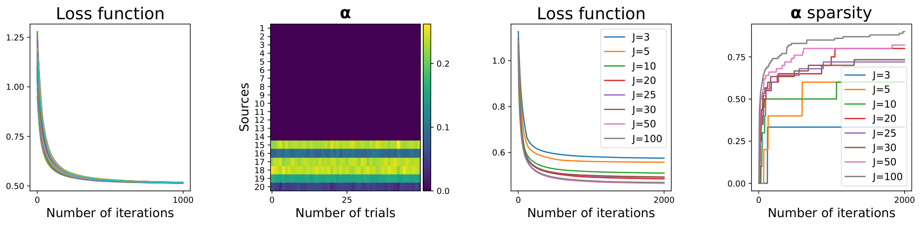
Algorithm convergence and stability In Figure 2 (Left and Center-left) we show the stability of the algorithm for different weights initialization. The loss function always converges and the coefficients are not affected by the initialization. Moreover, we observed in practice that choosing the same step for and does not degrade the performance and in all experiments we validated it via early stopping. We also noticed a fast convergence of the weights , meaning that the relevant domains are quickly identified. This behavior is illustrated in Fig. 2 (Right), where sparsity rapidly increases for any choice of illustrating that only few relevant source distributions are used in practice. We also report the loss convergence for increasing number of sources (Center-right).
Simulated Data: Domain Shift
We consider a classification problem similar to what is illustrated in Figure 1, but with 3 classes, i.e. , and in 3D. For the sources and target we generate and samples from Gaussian distributions rotated of angle around the -axis. As the data is already linearly separated, we set as the identity function in this experiment. We carried out many experiments in order to see the effect of different parameters such as the number of source domains , of source samples and of target samples . Each experiment has been repeated 50 times.
We report in Fig. 3 the accuracy of all methods with for (Left) and (Right). All competing methods are clearly outperformed by MSDA-WJDOT both in term of performance and variance even for a limited number of sources. Interestingly MSDA-WJDOT can even outperform Target due to its access to a larger number of samples. Another important aspect of MSDA-WJDOT is the obtained weights that can be used for interpretation. We show in Fig. 3 the weights that are attributed to the sources (ordered on the -axis by increasing rotation angles), for in an increasing rotation angle in the target samples (-axis). The estimated weights tend to be sparse and put more mass on sources that have a similar angle i.e. we recover automatically the closest sources in the joint distribution manifold. Note that we only report the method’s performances on those two configurations; the results for other experiments can be found in the supplementary material.
We next investigate how the function in (6) behaves when the weights are optimized w.r.t. the first term of the bound in Theorem 1. To this end we computed for sources an upper bound of with the - loss by using the estimated instead of the minimizer in
(6). We recover a value of that is very close to twice the Bayes error, corresponding to the best possible value for in this experiment. On the other hand, the value for the upper bound of for a uniform is and in average for 10000 randomly drawn values of . This suggests that optimizing with MSDA-WJDOT leads to a minimization of in the generalization bound.

Simulated Data: Target Shift We take into account the target shift problem with 2D source and target datasets which present different proportions of classes. The proportion of the class in the source is defined as (and similarly for the target). We consider a binary classification task and we sample sources and target datasets from the same Gaussian distribution. In Fig. 4 (Left and Center) we illustrate two sources and target distributions and how MSDA-WJDOT reweights the sources. As we can see, almost all the mass is concentrated on Source 2 () because its class proportion is closer to the target one. Instead, Source 1 has a class proportion inverted w.r.t. the target. In the experiment reported in Fig. 4 (Center-Right and Right) we have sources with randomly generated between and (we ordered the sources s.t. ). We show the average classification accuracy and the weights over 50 trials for varying in . Our method always outperforms JCPOT and selects the sources with a proportion of classes closer to the one in the target.
Object Recognition
The Caltech-Office dataset [Gong et al. 2012] contains four different domains: Amazon, Caltech [Griffin et al. 2007],
Webcam and DSLR. The variability of the different domains come from several factors: presence/absence of background, lightning conditions, noise, etc. We use for the embedding function the output of the 7th layer of a pre-trained DeCAF model [Donahue et al. 2014], similarly to what was done in Courty et al. 2016, resulting into an embedding space . For , we employ a one-layer neural network. Training is performed with Adam optimizer with 0.9 momentum and . Learning rate and regularization on the parameters are validated for all methods. In JDOT extensions and MSDA-WJDOT, we also validate the parameter weighting the feature distance in the cost (3).
The aim of this experiment is to evaluate MSDA-WJDOT and compare it with the current literature in the setting in which the embedding is given. The performance of the methods is reported in Table 1. We can see that MSDA-WJDOT is state of the art providing the best Average Rank (AR). Note that the DeCAF pre-trained embedding was originally designed in part to minimize the divergence across domains which as discussed is not the best configuration for MSDA-WJDOT but it still performs very well showing the robustness of MSDA-WJDOT to the embedding.
Moreover, we observed that for each adaptation problem MSDA-WJDOT provides one-hot vector (reported in supplementary) suggesting that only one source is needed for the target adaptation. Interestingly the source selected by MSDA-WJDOT for each target is the one that was reported with the best performance for single-source DA in Courty et al. 2016, which shows that MSDA-WJDOT can automatically find the relevant sources with no supervision.
| Method | Amazon | dslr | webcam | Caltech10 | AR |
| Baseline | 5.00 | ||||
| IWERM | 2.75 | ||||
| CJDOT | 3.50 | ||||
| MJDOT | 3.00 | ||||
| JCPOT∗ | 5.50 | ||||
| WBT∗ | 7.25 | ||||
| WBT | 4.00 | ||||
| MSDA-WJDOT | 2.25 | ||||
| Target | - | ||||
| Baseline+Target | - |
Music-speech Discrimination We now tackle a MSDA problem in which both the embedding and the target classifier need to be learned. Specifically, we consider the music-speech discrimination task introduced in Tzanetakis and Cook 2002, which includes 64 music and speech tracks of 30 seconds each. We generated 14 noisy datasets by combining the raw tracks with different types of noises from a noise dataset (spib.linse.ufsc.br/noise.html). The noisy datasets have been synthesised by PyDub python library [Robert et al. 2018]. We then used the libROSA python library [Brian McFee et al. 2015] to extract 13 MFCCs, computed every 10ms from 25ms Hamming windows followed by a z-normalization per track. We chose each of the four noisy datasets F16, Bucaneer2 (B2), Factory2 (F2), and Destroyerengine (D) as target domains, considering the remaining noisy datasets and the clean dataset as labelled source domains. The feature extraction is a Bidirectional Long Short-Term Memory (BLSTM) recurrent network with 2 hidden layers of 50 memory blocks each. The classifier is learned as one feed-forward layer. Model and training details are reported in the supplementary materials.
We report in Table 2, the mean and standard deviation accuracy on the testing set of each target dataset over 50 trials, as well as the Average Rank for each method. First note that on this hard adaptation problem the Baseline+Target approach only slightly improves the Baseline, and most of the methods performance shows large variance. As expected, MSDA-WJDOTMTL significantly outperforms MSDA-WJDOT confirming the importance of estimating an embedding exploiting the source variability. MSDA-WJDOTMTL achieves a 1.25 Average Rank outperforming all the other MSDA methods and also presents low standard deviation, showing robustness to small sample size. Surprisingly, MSDA-WJDOTMTL even outperforms both the Target and Baseline+Target methods, where the labels are available.
| Method | F16 | B2 | F2 | D | AR |
| Baseline | 9.25 | ||||
| IWERM | 8.75 | ||||
| IWERMMTL | 4.00 | ||||
| DCTN | 6.50 | ||||
| M3SDA | 8.50 | ||||
| CJDOT | 9.75 | ||||
| CJDOTMTL | 3.25 | ||||
| MJDOT | 9.50 | ||||
| MJDOTMTL | 3.50 | ||||
| JCPOT∗ | 5.50 | ||||
| WBT∗ | 11.75 | ||||
| WBT | 3.00 | ||||
| MSDA-WJDOT | 7.00 | ||||
| MSDA-WJDOTMTL | 2.25 | ||||
| Target | - | ||||
| Baseline+Target | - |
5 Conclusion
We presented a novel approach for multi-source DA that relies on OT for propagating labels from the sources and a weighting of the source domains that selects the best sources for the target task at hand in order to get a better prediction. We provided results that show that the proposed approach is theoretically grounded. We present numerical experiments on simulated data that shows the effectiveness of our method on both domain and target shift problems. Finally, we illustrate the good performance of MSDA-WJDOT on real-world benchmark datasets. Future works will investigate a regularization of and estimating simultaneously the embedding with MSDA-WJDOT instead of pre-training it with multitask learning. The embedding could indeed be updated for each new target which suggests an incremental formulation for MSDA-WJDOT that could be valuable in practice.
Acknowledgements
This work was partially funded through the 3IA Cote d’Azur Investments ANR-19-P3IA-0002 of the French National Research Agency (ANR), the DECIPHER-ASL – Bando PRIN 2017 grant (2017SNW5MB - Ministry of University and Research, Italy), and a grant from SAP SE and 5x1000, assigned to the University of Ferrara - tax return 2017. This research was produced within the framework of Energy4Climate Interdisciplinary Center (E4C) of IP Paris and Ecole des Ponts ParisTech. This research was supported by 3rd Programme d’Investissements d’Avenir ANR-18-EUR-0006-02. This action benefited from the support of the Chair "Challenging Technology for Responsible Energy" led by l’X – Ecole polytechnique and the Fondation de l’Ecole polytechnique, sponsored by TOTAL.
References
- Arjovsky et al. [2017] Martin Arjovsky, Soumith Chintala, and Léon Bottou. Wasserstein generative adversarial networks. In International conference on machine learning, pages 214–223. PMLR, 2017.
- Ben-David et al. [2010] Shai Ben-David, Tyler Lu, Teresa Luu, and Dávid Pál. Impossibility theorems for domain adaptation. In International Conference on Artificial Intelligence and Statistics, pages 129–136, 2010.
- Bolley et al. [2007] François Bolley, Arnaud Guillin, and Cédric Villani. Quantitative concentration inequalities for empirical measures on non-compact spaces. Probability Theory and Related Fields, 137(3-4):541–593, 2007.
- Brian McFee et al. [2015] Brian McFee, Colin Raffel, Dawen Liang, Daniel P.W. Ellis, Matt McVicar, Eric Battenberg, and Oriol Nieto. librosa: Audio and Music Signal Analysis in Python. In Proceedings of the 14th Python in Science Conference, pages 18 – 24, 2015.
- Caruana [1997] Rich Caruana. Multitask Learning. Machine Learning, 28(1):41–75, 1997.
- Courty et al. [2016] N. Courty, R. Flamary, D. Tuia, and A. Rakotomamonjy. Optimal transport for domain adaptation. Pattern Analysis and Machine Intelligence, IEEE Transactions on, 2016.
- Courty et al. [2017] Nicolas Courty, Rémi Flamary, Amaury Habrard, and Alain Rakotomamonjy. Joint distribution optimal transportation for domain adaptation. In Advances in Neural Information Processing Systems 30, pages 3730–3739. 2017.
- Cuturi [2013] Marco Cuturi. Sinkhorn distances: Lightspeed computation of optimal transport. In Advances in Neural Information Processing Systems, 2013.
- Damodaran et al. [2018] Bharath Bhushan Damodaran, Benjamin Kellenberger, Remi Flamary, Devis Tuia, and Nicolas Courty. DeepJDOT: Deep Joint Distribution Optimal Transport for Unsupervised Domain Adaptation. In ECCV 2018 - 15th European Conference on Computer Vision, volume 11208, pages 467–483, 2018.
- Donahue et al. [2014] Jeff Donahue, Yangqing Jia, Oriol Vinyals, Judy Hoffman, Ning Zhang, Eric Tzeng, and Trevor Darrell. Decaf: A deep convolutional activation feature for generic visual recognition. In International conference on machine learning, pages 647–655, 2014.
- Fatras et al. [2020] Kilian Fatras, Younes Zine, Rémi Flamary, Remi Gribonval, and Nicolas Courty. Learning with minibatch wasserstein: asymptotic and gradient properties. In Proceedings of the Twenty Third International Conference on Artificial Intelligence and Statistics, volume 108 of Proceedings of Machine Learning Research, pages 2131–2141, 2020.
- Flamary et al. [2021] Rémi Flamary, Nicolas Courty, Alexandre Gramfort, et al. Pot: Python optimal transport. Journal of Machine Learning Research, 22(78):1–8, 2021.
- Ganin et al. [2016] Yaroslav Ganin, Evgeniya Ustinova, Hana Ajakan, et al. Domain-adversarial training of neural networks. Journal of Machine Learning Research, 17(1):2096–2030, 2016.
- Genevay et al. [2018] Aude Genevay, Gabriel Peyré, and Marco Cuturi. Learning generative models with sinkhorn divergences. In International Conference on Artificial Intelligence and Statistics, pages 1608–1617. PMLR, 2018.
- Ghifary et al. [2016] Muhammad Ghifary, W. Bastiaan Kleijn, Mengjie Zhang, David Balduzzi, and Wen Li. Deep reconstruction-classification networks for unsupervised domain adaptation. CoRR, abs/1607.03516, 2016.
- Gong et al. [2012] Boqing Gong, Yuan Shi, Fei Sha, and Kristen Grauman. Geodesic flow kernel for unsupervised domain adaptation. In CVPR, pages 2066–2073. IEEE Computer Society, 2012.
- Griffin et al. [2007] G. Griffin, A. Holub, and P. Perona. Caltech-256 object category dataset. Technical Report 7694, California Institute of Technology, 2007.
- Held et al. [1974] Michael Held, Philip Wolfe, and Harlan P Crowder. Validation of subgradient optimization. Mathematical programming, 6(1):62–88, 1974.
- Hoffman et al. [2018] Judy Hoffman, Mehryar Mohri, and Ningshan Zhang. Algorithms and theory for multiple-source adaptation. In Advances in Neural Information Processing Systems, pages 8246–8256, 2018.
- Jiang [2008] Jing Jiang. A literature survey on domain adaptation of statistical classifiers. URL: http://sifaka. cs. uiuc. edu/jiang4/domainadaptation/survey, 3(1-12):3, 2008.
- Kantorovich [1942] Leonid V Kantorovich. On the translocation of masses. In Dokl. Akad. Nauk. USSR (NS), volume 37, pages 199–201, 1942.
- Kouw and Loog [2019] Wouter M Kouw and Marco Loog. A review of domain adaptation without target labels. IEEE transactions on pattern analysis and machine intelligence, 43(3):766–785, 2019.
- Lin et al. [2020] Chuang Lin, Sicheng Zhao, Lei Meng, and Tat-Seng Chua. Multi-source domain adaptation for visual sentiment classification. In Proceedings of the AAAI Conference on Artificial Intelligence, volume 34, pages 2661–2668, 2020.
- Long et al. [2016] Mingsheng Long, Han Zhu, Jianmin Wang, and Michael I Jordan. Unsupervised domain adaptation with residual transfer networks. Advances in neural information processing systems, 29, 2016.
- Mansour et al. [2009] Yishay Mansour, Mehryar Mohri, and Afshin Rostamizadeh. Domain adaptation with multiple sources. In Advances in neural information processing systems, pages 1041–1048, 2009.
- Monge [1781] Gaspard Monge. Mémoire sur la théorie des déblais et de remblais. In Histoire de l’Académie Royale des Sciences de Paris, avec les Mémoires de Mathématique et de Physique pour la même année. 1781.
- Montesuma and Mboula [2021] Eduardo Fernandes Montesuma and Fred Maurice Ngole Mboula. Wasserstein barycenter for multi-source domain adaptation. In Proceedings of the IEEE/CVF Conference on Computer Vision and Pattern Recognition, pages 16785–16793, 2021.
- Nguyen et al. [2021a] Tuan Nguyen, Trung Le, He Zhao, Quan Hung Tran, Truyen Nguyen, and Dinh Phung. Most: Multi-source domain adaptation via optimal transport for student-teacher learning. In Uncertainty in Artificial Intelligence, pages 225–235. PMLR, 2021a.
- Nguyen et al. [2021b] Van-Anh Nguyen, Tuan Nguyen, Trung Le, Quan Hung Tran, and Dinh Phung. Stem: An approach to multi-source domain adaptation with guarantees. In Proceedings of the IEEE/CVF International Conference on Computer Vision, pages 9352–9363, 2021b.
- Paszke et al. [2017] Adam Paszke, Sam Gross, Soumith Chintala, Gregory Chanan, Edward Yang, Zachary DeVito, Zeming Lin, Alban Desmaison, Luca Antiga, and Adam Lerer. Automatic differentiation in pytorch. 2017.
- Peng et al. [2019] Xingchao Peng, Qinxun Bai, Xide Xia, Zijun Huang, Kate Saenko, and Bo Wang. Moment matching for multi-source domain adaptation. In Proceedings of the IEEE/CVF international conference on computer vision, pages 1406–1415, 2019.
- Redko et al. [2017] Ievgen Redko, Amaury Habrard, and Marc Sebban. Theoretical analysis of domain adaptation with optimal transport. In Machine Learning and Knowledge Discovery in Databases - European Conference, ECML PKDD 2017, Proceedings, Part II, volume 10535, pages 737–753, 2017.
- Redko et al. [2019a] Ievgen Redko, Nicolas Courty, Rémi Flamary, and Devis Tuia. Optimal transport for multi-source domain adaptation under target shift. In Proceedings of Machine Learning Research, volume 89 of Proceedings of Machine Learning Research, pages 849–858. PMLR, 16–18 Apr 2019a.
- Redko et al. [2019b] Ievgen Redko, Nicolas Courty, Rémi Flamary, and Devis Tuia. Optimal transport for multi-source domain adaptation under target shift. In International Conference on Artificial Intelligence and Statistics (AISTAT), 2019b.
- Robert et al. [2018] James Robert, Marc Webbie, et al. Pydub, 2018.
- Shen et al. [2018] Jian Shen, Yanru Qu, Weinan Zhang, and Yong Yu. Wasserstein distance guided representation learning for domain adaptation. In Thirty-Second AAAI Conference on Artificial Intelligence, 2018.
- Sugiyama et al. [2007] Massahi Sugiyama, Matthias Krauledat, and Klaus-Robert Muller. Covariate shift adaptation my importance weighted cross validation. Journal of Machine Learning Research, 8:985–1005, December 2007.
- Sun and Saenko [2016] Baochen Sun and Kate Saenko. Deep coral: Correlation alignment for deep domain adaptation. In European Conference on Computer Vision, pages 443–450, 2016.
- Tzanetakis and Cook [2002] George Tzanetakis and Perry Cook. Musical genre classification of audio signals. IEEE Transactions on Speech and Audio Processing, 2002.
- Tzeng et al. [2014] Eric Tzeng, Judy Hoffman, Ning Zhang, Kate Saenko, and Trevor Darrell. Deep domain confusion: Maximizing for domain invariance. CoRR, abs/1412.3474, 2014.
- Tzeng et al. [2015] Eric Tzeng, Judy Hoffman, Trevor Darrell, and Kate Saenko. Simultaneous deep transfer across domains and tasks. In Proceedings of the IEEE international conference on computer vision, pages 4068–4076, 2015.
- Tzeng et al. [2017] Eric Tzeng, Judy Hoffman, Kate Saenko, and Trevor Darrell. Adversarial discriminative domain adaptation. In The IEEE Conference on Computer Vision and Pattern Recognition (CVPR), 2017.
- Wen et al. [2020] Junfeng Wen, Russell Greiner, and Dale Schuurmans. Domain aggregation networks for multi-source domain adaptation. In Proc. 37th International Conference on Machine Learning, volume 119 of Proceedings of Machine Learning Research, pages 10214–10224, 2020.
- Wu et al. [2019] Yifan Wu, Ezra Winston, Divyansh Kaushik, and Zachary Lipton. Domain adaptation with asymmetrically-relaxed distribution alignment. In Proc.36th International Conference on Machine Learning, volume 97 of Proceedings of Machine Learning Research, pages 6872–6881, 2019.
- Xu et al. [2018] Ruijia Xu, Ziliang Chen, Wangmeng Zuo, Junjie Yan, and Liang Lin. Deep cocktail network: Multi-source unsupervised domain adaptation with category shift. 2018 IEEE/CVF Conference on Computer Vision and Pattern Recognition, 2018.
- Zhao et al. [2018] Han Zhao, Shanghang Zhang, Guanhang Wu, et al. Adversarial multiple source domain adaptation. In Advances in neural information processing systems, pages 8559–8570, 2018.
- Zhao et al. [2019] Han Zhao, Remi Tachet Des Combes, Kun Zhang, and Geoffrey Gordon. On learning invariant representations for domain adaptation. In Proceedings of the 36th International Conference on Machine Learning, volume 97 of Proceedings of Machine Learning Research, pages 7523–7532, 2019.
Supplementary Material
The supplementary material is organized as follows. In Section A we provide proof of Lemma 1, Lemma 2 and Theorem 1. For reader’s convenience the results are repeated in this supplementary material. Section B recalls the MSDA-WJDOT algorithm and defines the projection to the simplex implemented in the algorithm. Finally, in Section C we present additional numerical experiments.
Appendix A Proofs
A.1 Proof of Lemma 1
Lemma 1.
For any hypothesis , denote as and , the expected loss of on the target and on the weighted sum of the source domains, with respect to a loss function bounded by . We have
| (9) |
where is a convex combination of the source distributions with weights , and is the total variation distance.
Proof.
We define the error of an hypothesis with respect to a loss function and a joint probability distribution as
then using simple arguments, we have
| (10) | ||||
and using the definition of the total variation distance between distribution we conclude the proof. ∎
A.2 Proof of Theorem 1
The proof of this theorem follows the same steps as the one proposed by Courty et al. 2017 and we reproduce it here for a sake of completeness.
Definition 1 (Probabilistic Transfer Lipschitzness – PLT Property).
Let and be respectively the source and target distributions. Let . A labeling function and a joint distribution over and are -Lipschitz transferable if for all , we have
with being a metric on .
This property provides a bound on the probability of finding a couple of source-target examples that are differently labeled in a -ball with respect to and the metric .
Definition 2.
(Similarity measure) Let be a space of -Lipschitz labelling functions. Assume that, for every and , . The similarity between and can defined [Ben-David et al. 2010, Def. 5] as
| (11) |
where the risk is measured w.r.t. to a symmetric and -Lipschitz loss function that satisfies the triangle inequality.
Lemma 2.
Proof.
We have that
where the second equality comes from the symmetry of the loss function and the third one is due to the fact that since the label is not used in the expectation.
Now, we analyze the first term in the r.h.s. of the last inequality. Note that samples drawn from distribution can be expressed as with .
| (13) | ||||
| (14) | ||||
| (15) | ||||
| (16) | ||||
| (17) |
Inequality in line (13) is due to the Kantorovitch-Rubinstein theorem stating that for any coupling the following inequality holds
followed by an application of the triangle inequality. Since, the above inequality applies for any coupling, it applies also for . Inequality (14) is due to the assumption that the loss function is -Lipschitz in its second argument. Inequality (15) derives from the PTL property with probability of and . In addition, taking into account that the difference between two samples with respect to is bounded by , we have the term that covers the regions where PTL assumption does not hold. Inequality (16) is obtained from the symmetry of , the triangle inequality on the loss and by posing . ∎
First we need to prove the following Lemma.
Lemma 3.
For any distributions and in the simplex we have
Proof.
First we recall that the Wasserstein Distance between two distribution is
| (18) |
where . Let be the optimal OT matrix between and . It is obvious to see that respects the marginal constraints for , i.e. . Hence, is a feasible solution for the OT problem and, consequently, the cost for this feasible solution is greater or equal than the optimal value . Since we recover the Lemma above. ∎
We can now prove Theorem 1, which we also restate for the convenience of the reader.
Theorem 1.
Under the assumptions of Lemma 2, let be -th source empirical distributions of samples and the empirical target distribution with samples. Then for all , with in the ground metric we have with probability
| (19) |
Proof.
By the triangle inequality we have that
where the last inequality follows from Lemma 3. Using the well known convergence property of the Wasserstein distance proven in Bolley et al. 2007 we find the following bound with probability
| (20) |
with corresponding to all source and target distributions under similar conditions as in Courty et al. 2017. ∎
Appendix B The algorithm
We recall here the algorithm we proposed to solve the MSDA-WJDOT problem (Algorithm 2). is the projection to the simplex defined as
| (21) |
We implemented it by using Algorithm 3, firstly proposed in Held et al. 1974.
Appendix C Numerical experiments
C.1 Simulated data
Domain shift
We generate a data set by drawing from a 3-dimensional Gaussian distribution with 3 cluster centers and standard deviation . We keep the same number of examples for each cluster. To simulate the sources, we apply rotations to the input data around the -axis. More precisely, we draw equispaced angles from and we get as
| (22) |
To generate the target domain , we follow the same procedure by randomly choosing an angle . We keep the label set fixed, i.e. . Note that in this case the embedding function is the identity function and, hence, . In the following we report all the experiment we carried out on the simulated data, in which we also investigate to replace the exact Wasserstein distance by the the Bures-Wasserstein distance
| (23) |
where the are respectively the first and second order moments of distribution (and similarly for ). The BW distance has the advantage of having a complexity linear in the number of samples that can scale better to large dataset.
We label this method variant with , while we refer to the exact OT as .
In the following, we investigate the performance of MSDA-WJDOT at varying of the number of sources , source samples , and target samples . We compare the proposed approch with other MSDA methods and with the Baseline, Target, Bayes classification.
- •
Varying the number of sources: we keep the number of samples fixed in both sources and target datasets (s.t. ) and we vary the number of sources . In Fig. 6 we report the accuracy of the different methods.
Figure 5: Methods’ accuracy for varying the number of sources . Figure 6: Methods’ accuracy for varying the number of source samples. Figure 7: Methods’ accuracy for varying the number of target samples Figure 8: Methods’ accuracy for varying the number of source and target samples 
Figure 9: Recovered with small sample size (). 
Figure 10: Recovered for . - •
- •
Varying the number of the target samples: we fix and , with . We let vary the number of target samples in (Fig. 8).
- •
Varying the number of samples of all domains: we fix the number of sources equal to 20. We let vary the number of source and target samples in , by keeping with . We report the methods’ accuracy in Fig. 6.
In all experiments MSDA-WJDOT significantly outperfoms CJDOT, MJDOT, IWERM and the Baseline. Both MSDA-WJDOT(E) and MSDA-WJDOT(B) provide a better or at least comparable performance w.r.t. the Target method, in which the labels of the target dataset are used. In Fig. 10 and 10 we show the recovered weights for and , respectively. In both cases, the - axis reports different random target angles in the interval (ordered by increasing angles), whereas the -axis represents the source angles ordered such that , . As we can see, the weights are higher along the diagonal meaning that MSDA-WJDOT always rewards the sources with angle closest to .


C.2 Real data
In the section, we introduce a new strategy for the validation, in alternative to the one based on SSE proposed in Sec. 3.2. We propose to employ the accuracy of the learned classifier on the source datasets and weighted by , i.e.
| (24) |
with . To refer to this approach, we denote as MSDA-WJDOTacc, CJDOTacc, MJDOTacc the MSDA-WJDOT and the two JDOT extensions respectively. Let us remark that MSDA-WJDOTacc is a way to reuse the weights that provide the closest source distributions which, hence, are supposed to give a better estimate of the performance of the current classifier.
Object recognition
In Table 3 we report the source weights provided by MSDA-WJDOT. In all cases, is a one-hot vector suggesting that only one source is meaningfully related to the target domain. This is in line with the results on single-source DA found in Courty et al. 2016 in which the source domain providing the highest accuracy corresponds to the one selected by MSDA-WJDOT.
| Target | Amazon | dslr | webcam | Caltech10 |
|---|---|---|---|---|
| Amazon | - | 0 | 0 | 1 |
| dslr | 0 | - | 1 | 0 |
| webcam | 0 | 1 | - | 0 |
| Caltech10 | 1 | 0 | 0 | - |
Table 4 is a full version of Table 1 in the paper, in which we also show the accuracy obtained by employing the validation strategy introduced in Eq. 24. We can observe that MSDA-WJDOTacc provides good performances, comparable with both MSDA-WJDOT and the other MSDA methods, but MSDA-WJDOT still remains the state of the art.
| Method | Amazon | dslr | webcam | Caltech10 | AR |
| Baseline | 6.75 | ||||
| IWERM Sugiyama et al. 2007 | 3.25 | ||||
| CJDOTacc Courty et al. 2017 | 4.50 | ||||
| CJDOT Courty et al. 2017 | 4.50 | ||||
| MJDOTacc Courty et al. 2017 | 3.75 | ||||
| MJDOT Courty et al. 2017 | 4.50 | ||||
| JCPOT∗ Redko et al. 2019a | 7.25 | ||||
| WBT∗ Montesuma and Mboula 2021 | 9.50 | ||||
| WBT Montesuma and Mboula 2021 | 5.00 | ||||
| MSDA-WJDOTacc | 4.25 | ||||
| MSDA-WJDOT | 2.75 | ||||
| Target | - | ||||
| Baseline+Target | - |
Music-speech discrimination

The model we adopted is shown in Fig. 12, where is a two-layers Bidirectional Long Short-Term Memory (BLSTM) that feeds the one feed-forward layer with the last hidden state. Weights were initialized with Xavier initialization. Training is performed with Adam optimizer with 0.9 momentum and . Learning rate exponentially decays every epoch. We grid-research the initial learning rate value and the decay rate.
In Table 5 we show the MSDA performances in the music-speech discrimination. In particular, for MSDA-WJDOT and JDOT variants the validation strategy described in formula 24 has been employed. Results show that, although this is a valid strategy, early stopping based on SSE described in Sec. 4 always outperforms. The Average Rank shows that MSDA-WJDOT is state of the art in music-speech discrimination.
| Method | F16 | Buccaneer2 | Factory2 | Destroyerengine | AR |
| Baseline | 11.25 | ||||
| IWERM Sugiyama et al. 2007 | 10.75 | ||||
| IWERMmtl Sugiyama et al. 2007 | 5.50 | ||||
| DCTN Xu et al. 2018 | 8.50 | ||||
| M3SDA Peng et al. 2019 | 10.25 | ||||
| CJDOT Courty et al. 2017 | 11.50 | ||||
| CJDOTmtl Courty et al. 2017 | 4.00 | ||||
| CJDOT Courty et al. 2017 | 3.50 | ||||
| MJDOTCourty et al. 2017 | 11.50 | ||||
| MJDOTmtlCourty et al. 2017 | 4.00 | ||||
| MJDOTCourty et al. 2017 | 4.75 | ||||
| JCPOT∗Redko et al. 2019a | 7.50 | ||||
| WBT∗Montesuma and Mboula 2021 | 13.00 | ||||
| WBTMontesuma and Mboula 2021 | 4.25 | ||||
| MSDA-WJDOT | 8.00 | ||||
| MSDA-WJDOTmtl | 2.75 | ||||
| MSDA-WJDOT | 3.50 | ||||
| MSDA-WJDOTacc | 8.00 | ||||
| Target | - | ||||
| Baseline+Target | - |