Anisotropic Stark shift, field-induced dissociation, and electroabsorption of excitons in phosphorene
Abstract
We compute binding energies, Stark shifts, electric-field-induced dissociation rates, and the Franz-Keldysh effect for excitons in phosphorene in various dielectric surroundings. All three effects show a pronounced dependence on the direction of the in-plane electric field, with the dissociation rates in particular decreasing by several orders of magnitude upon rotating the electric field from the armchair to the zigzag axis. To better understand the numerical dissociation rates, we derive an analytical approximation to the anisotropic rates induced by weak electric fields, thereby generalizing the previously obtained result for isotropic two-dimensional semiconductors. This approximation is shown to be valid in the weak-field limit by comparing it to the exact rates. The anisotropy is also apparent in the large difference between armchair and zigzag components of the exciton polarizability tensor, which we compute for the five lowest lying states. As expected, we also find much more pronounced Stark shifts in either the armchair or zigzag direction, depending on the symmetry of the state in question. Finally, an isotropic interaction potential is shown to be an excellent approximation to a more accurate anisotropic interaction derived from the Poisson equation, confirming that the anisotropy of phosphorene is largely due to the direction dependence of the effective masses.
I Introduction
With the experimental discovery of graphene in 2004 Novoselov et al. 2004, interest in two-dimensional (2D) materials increased enormously. Just a few years later, the successful exfoliation of monolayer MoS2 Mak et al. 2010 produced the first atomically thin direct band gap semiconductor. One of the newest members of the 2D semiconductor family is monolayer black phosphorus (BP), referred to here as phosphorene Li et al. 2014; Koenig et al. 2014; Liu et al. 2014; Castellanos-Gomez et al. 2014; Xia et al. 2014a. It has seen a remarkable rate of growth in research interest, even more so than graphene Castellanos-Gomez 2015. Unlike transition metal dichalcogenides (TMDs), where the band gap is direct only in their monolayer form Chhowalla et al. 2013, BP is a direct band gap semiconductor regardless of the number of layers Keyes 1953; Asahina and Morita 1984; Morita 1986; Rudenko and Katsnelson 2014. The magnitude of the gap evolves from around eV in its bulk form to around eV in monolayers Castellanos-Gomez et al. 2014; Qiao et al. 2014; Tran et al. 2014; Liu et al. 2014; Wang et al. 2015. The extreme tunability of the band gap, as well as its highly anisotropic nature, make phosphorene an exceptionally interesting material for both practical applications and theoretical investigation. For instance, the tunable gap makes phosphorene a promising material for converting solar energy to chemical energy Hu et al. 2016. The anisotropy of phosphorene shows up in almost all of its physical properties, such as its electrical Fei and Yang 2014; Xu et al. 2015, thermal Ong et al. 2014; Jain and McGaughey 2015, and mechanical Wei and Peng 2014 properties. Particular examples of highly anisotropic quantities in phosphorene are the conductivity Xia et al. 2014b, optical absorption Xia et al. 2014a, and photoluminescence Wang et al. 2015.
Very strong absorption peaks have been observed in monolayer and bilayer phosphorene Liu et al. 2014; Zhang et al. 2014, due to strongly bound excitons Tran et al. 2014; Rodin et al. 2014; Hunt et al. 2018; Henriques and Peres 2020. How such strongly bound excitons interact with external electric fields is an interesting area of study, particularly in phosphorene as the direction of the in-plane field will matter. An applied electric field pulls electrons and holes in opposite directions, which causes a shift in the exciton energy and may even lead to dissociation of the exciton. Collectively, these effects have been studied intensely in carbon nanotubes Perebeinos and Avouris 2007; Mohite et al. 2008; Kamban et al. 2020, as well as monolayer Pedersen 2016; Haastrup et al. 2016; Scharf et al. 2016; Massicotte et al. 2018; Cavalcante et al. 2018; Kamban and Pedersen 2019, bilayer Kamban and Pedersen 2020, and multilayer TMDs Pedersen et al. 2016a. They have been studied to a lesser degree in phosphorene Chaves et al. 2015; Cavalcante et al. 2018, where focus has been on the energy shift rather than field-induced exciton dissociation. One of the motivations for applying external electric fields to low-dimensional semiconductors from a device perspective is to induce exciton dissociation, and thereby improve photocurrent generation in, e.g., solar cells and photodetectors. The exciton Stark effect is also promising as a means of manipulating the properties of semiconductors. For instance, the shift in exciton energy and possibility of dissociation caused by an applied field shifts and broadens the optical absorption peaks. This is known as the Franz-Keldysh effect Franz 1958; Keldysh 1958, and was studied for monolayer TMDs in Ref. Pedersen 2016. In TMDs, both Stark and Franz-Keldysh effects are independent of the direction of an in-plane electric field. In contrast, the highly anisotropic nature of phosphorene leads to a Stark effect that is strongly dependent on the direction of the field Chaves et al. 2015; Cavalcante et al. 2018, and this effect should also be visible in the Franz-Keldysh effect.
In the present paper, we study the exciton Stark and Franz-Keldysh effects in phosphorene. The paper is structured as follows. In section II, we introduce the model used and show that using an isotropic interaction potential between the electron and hole is an excellent approximation to a more accurate anisotropic interaction. For phosphorene, the majority of the anisotropy therefore comes from the direction dependent effective masses. In this section, we also compute the energies of the five lowest lying exciton states in phosphorene in three different dielectric surroundings and discuss their symmetries. In section III, the focus is on the exciton Stark effect. Here we observe Stark shifts and exciton dissociation rates that are strongly dependent on the direction of the field. To better understand these effects, we compare the Stark shifts and dissociation rates to analytical approximations derived from perturbation theory and weak-field asymptotic theory (WFAT), respectively. In section IV, we turn to the Franz-Keldysh effect, which also exhibits pronounced direction dependence. Finally, the results are concluded upon in section V. The text is supplemented by two appendices. In appendix A, the exciton interaction potential in an anisotropic semiconductor is discussed, and in appendix B, an anisotropic weak-field approximation for the exciton dissociation rate is derived.
II Excitons in phosphorene

By now, it is well known that many excitonic effects are accurately described by modeling the excitons as electron-hole pairs satisfying the Wannier equation Wannier 1937; Lederman and Dow 1976. It has been shown repeatedly that the Wannier model reproduces the exciton binding energies obtained from first principle calculations to a satisfactory degree Cudazzo et al. 2010; Pulci et al. 2012; Latini et al. 2015; Henriques et al. 2019. This is fortunate, as first principle calculations require solving the computationally demanding Bethe-Salpeter equation Salpeter and Bethe 1951; Onida et al. 2002. Importantly, the Wannier model has also been shown to agree with experimental results for the exciton Stark effect, field-induced dissociation, and the Franz-Keldysh effect Massicotte et al. 2018. For anisotropic 2D semiconductors, the Wannier equation in the absence of an electric field reads (in atomic units)
| (1) |
where is the electron-hole interaction, the energy, and
| (2) |
is the direction-specific reduced mass with and being the electron and hole effective masses along the -direction, respectively. The exciton interaction in anisotropic semiconductors is, of course, anisotropic. It may be found by modeling the encapsulated 2D semiconductor (depicted in fig. 1 (a) ) as a three-layer structure with a piecewise constant dielectric function, and then solving the Poisson equation for two charges in this structure. This is done in appendix A. For a superstrate, a 2D semiconductor, and a substrate with dielectric tensors , , and , respectively, we find with a linearized dielectric function
| (3) |
where , , and . The screening lengths are defined as and , where and are the 2D sheet polarizabilities in the - and -direction, respectively. These are the microscopic definitions of the screening lengths Berkelbach et al. 2013. The macroscopic definitions may be seen in appendix A. Note that eq. 3 reduces to the usual Rytova-Keldsyh potential Rytova 1967; Keldysh 1979; Trolle et al. 2017 in the isotropic case.
The polarizabilities for phosphorene were computed in Ref. Rodin et al. 2014, where the authors found and . These values are quite close, which in turn leads to a very weak angular contribution to the interaction. As a first approximation, we may therefore consider only the leading term. Further expanding to first order in , we find the Rytova-Keldysh form Rytova 1967; Keldysh 1979
| (4) |
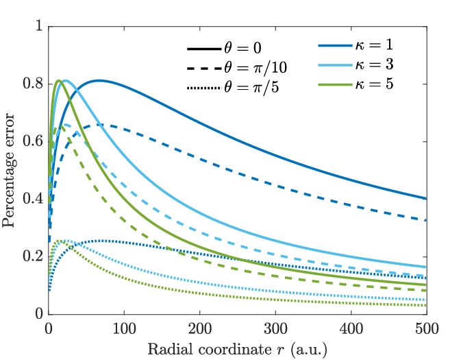
with . This form agrees with the interaction used by many authors to study excitons in phosphorene Rodin et al. 2014; Faria Junior et al. 2019; Henriques and Peres 2020. Using the isotropic approximation to describe the excitons is justified by noting that it agrees with the full potential in eq. 3 to within for all and . Errors for three different dielectric surroundings and field directions are shown in fig. 2. As is evident, these errors are low, and they decrease as tends to , as the dominating angular contribution from the term tends to zero in this region. The parameters used to describe excitons in phosphorene in the present paper are summarized in table 1.
| State | State | State | State | ||||
|---|---|---|---|---|---|---|---|
| About -axis | Even | Even | Odd | Odd | |||
| About -axis | Even | Odd | Odd | Even | |||
| About origin | Even | Odd | Even | Odd | |||
| Along -axis | - | - | 0 | 0 | |||
| Along -axis | - | 0 | 0 | - |
To perform numerical calculations, it is convenient to switch to the coordinates introduced in Ref. Rodin et al. 2014 defined by
| (5) |
This transforms eq. 1 into
| (6) |
with , and the polar representation of the -plane, and where the Laplacian is to be taken with respect to these coordinates. The transformation makes the kinetic energy isotropic at the cost of making the potential energy anisotropic. The reasons that this transformation is useful are threefold: firstly, it is more intuitive to work with an anisotropic potential than an anisotropic kinetic energy; secondly, the numerical procedure we shall use consists of resolving the wave function in a basis, and the number of basis functions needed to represent the polar wave function is significantly less than those needed to represent the Cartesian wave function; and, finally, the polar representation of the kinetic energy is simple, and thus leads to simple matrix elements. The states may be expressed generally as
| (7) |
where may be understood as the Fourier coefficients. Note that the coefficients depend continuously on , and will later be expanded in a radial basis. As pointed out in Ref. Rodin et al. 2014, the unperturbed eigenstates of eq. 6 fall into four distinct groups. This is most easily seen by recognizing that the potential is even in and is invariant under the shift . It therefore has a Fourier series consisting of cosines of even order, and it becomes easy to see that for coupling to occur, the angular functions must be of the same type (i.e. sine/cosine) and have the same angular momentum parity. This results in the following four types of states
| (8) | ||||
| (9) | ||||
| (10) | ||||
| (11) |
where the subscripts and denote whether the trigonometric function is a cosine/sine and whether the angular momentum parity is even/odd, respectively. A couple of symmetry observations follow immediately and are summarized in table 2. Importantly, states with even and odd angular momenta are symmetric and antisymmetric about the origin, respectively. This means that the and states are necessarily zero at the origin, and are therefore not optically active when no external electric field is present, as we shall see later on when we compute the optical absorption. The shape of the states may be inferred from the fact that some of them have angular nodes along a specific axis. In particular, the and states have nodes along the - and -axis, respectively, and the state has nodes along both. They will therefore be slightly deformed versions of the familiar , , and orbitals.
The numerical procedure we will use throughout the paper is to solve the Wannier equation using a finite element representation of the exciton wave functions. The wave functions are expanded as in eq. 7, including angular momenta up to some number . The radial functions are then expanded in a finite element basis that are non-zero only on a single radial segment defining a particular range of the radial coordinate. Their exact form, as well as further detail of the numerical procedure can be found in Ref. Kamban and Pedersen 2019. To summarize,
| (12) |
where are the expansion coefficients obtained by solving the resulting matrix eigenvalue problem.
| Freely suspended | SiO2 substrate | hBN encapsulation | ||||
|---|---|---|---|---|---|---|
| Type | (meV) | (meV) | (meV) | |||
In the present paper, we will study phosphorene in three different dielectric environments. Namely, freely suspended (), on an SiO2 substrate (), and encapsulated by hBN (). The energy and symmetry of the five lowest lying states for the three dielectric surroundings are shown in table 3. As can be seen, we find exciton binding energies of , , and meV, respectively, which corresponds well with those presented in Refs. Rodin et al. 2014; Chaves et al. 2015; Yang et al. 2015; Hunt et al. 2018; Faria Junior et al. 2019; Henriques and Peres 2020 (see Ref. Henriques and Peres 2020 for a table summarizing the binding energies from more references). Additionally, the energies of the excited states are in good agreement with those found in Ref. Chaves et al. 2015. Note that the state is an state that has an angular node along the -axis. The fact that this state has a lower energy than the state can be understood by considering the potential in eq. 6. It is weaker along the -axis than it is along the -axis, thus favoring a state along . As a final note, the state is not among the first five states. That it has such a large energy is no surprise given its -like shape.
III Anisotropic exciton Stark effect
We are interested in seeing how the anisotropic nature of phosphorene affects both the exciton Stark shifts and dissociation rates when an in-plane electrostatic field is applied to the sheet. In the presence of an electric field, the Wannier equation reads
| (13) |
where is the electric field strength and its angle to the original -axis. The setup is pictured in fig. 1, where the field direction is indicated in panel (b). Applying a field to the exciton induces resonance states and, in turn, makes the energy eigenvalue complex Haastrup et al. 2016; Pedersen et al. 2016a. The Stark shift then corresponds to the change in the real part of the energy as a function of field strength, while the imaginary part describes the dissociation rate by the relation . This complex eigenvalue is most easily obtained by using the complex scaling procedure Balslev and Combes; Aguilar and Combes. Here, the radial coordinate is rotated into the complex plane, which transforms the diverging behavior of the resonance states for real into bound states along a complex contour .

The procedure we shall use here has been laid out in Ref. Kamban and Pedersen 2019, where we compute the exciton Stark effect in TMDs. It consists of expanding the resonance state in a finite element basis, as described above, and only complex scaling the coordinate outside a desired radius. This technique is referred to as exterior complex scaling Scrinzi and Elander 1993, and it makes it much easier to obtain the dissociation rates for weak fields numerically. The results for phosphorene in free space, on an SiO2 substrate, and encapsulated by hBN can be seen in the top, middle, and bottom panel of fig. 3, respectively. It is immediately clear that the field direction, indicated by the line color, is very important. This is in contrast to the effect in TMDs, which is fully isotropic Haastrup et al. 2016; Massicotte et al. 2018; Kamban and Pedersen 2019. The largest Stark shifts (left axis) and dissociation rates (right axis) are seen for fields pointing along the -axis, which coincides with the direction of lowest effective mass. Rotating the field from the -axis to the -axis reduces the dissociation rate by several orders of magnitude, due to the increased effective mass. The direction dependent Stark shifts and dissociation rates add an additional degree of freedom when using phosphorene in device design, as not only can they be controlled by the dielectric environment, but by the field direction as well. Taking a closer look at the effect of the dielectric surroundings, both the Stark shifts and dissociation rates increase significantly by placing the phosphorene sheet on an SiO2 substrate, and even more so by encapsulating it in hBN. This is to be expected, as the exciton binding energy is reduced considerably with increased screening. It should also be noted that the shifts and rates are much lower than those in popular TMDs Kamban and Pedersen 2019, which is a direct consequence of the larger binding energies of excitons in phosphorene.
III.1 Exciton Stark shift and polarizability
In this section, we shall look at the exciton Stark shift in more detail, and compare to the shift predicted by perturbation theory. The anisotropic exciton Stark shift in few layer BP in free space and in hBN surroundings was studied in Ref. Cavalcante et al. 2018, and on an SiO2 substrate in Ref. Chaves et al. 2015, and we shall thus make a detailed comparison to the results in these papers for a single layer of BP, i.e. phosphorene. One of the most important quantities describing how anisotropic excitons interact with the electric field is their polarizabilities. The perturbation series for the Stark shift of state may be written as Landau and Lifshitz 1989
| (14) |
with
| (15) |
and
| (16) |
where
| (17) |
and the sum is to be taken over all the unperturbed states. The perturbation only couples states with different parity angular momenta (see eqs. 8, 9, 10 and 11). The first order correction therefore immediately reduces to zero. The second order correction, on the other hand, may be written as
| (18) |
where the - and -components of the exciton polarizability tensor for the four types of states are given by
| (19) | |||
| (20) | |||
| (21) | |||
| (22) |
with the shorthand notation
| (23) | ||||
| (24) |
The finite element expansion described above is very flexible and perfectly capable of resolving both the bound and continuous spectrum of unperturbed states. In this manner, we compute the exciton polarizabilities for the five lowest lying exciton states. They are summarized in table 4, and a comparison between eq. 18 and the numerically exact Stark shifts is shown in fig. 4 for very weak fields. It is clear that all of the states have a highly anisotropic response to an applied field. We observe, as expected, that the -component of the polarizability is larger than the -component for the fundamental exciton. The opposite is the case for the states, which is of no surprise given their -like shape. Perhaps more surprisingly we find that the -component of the state is larger than the -component.

| Freely suspended | SiO2 substrate | hBN encapsulation | |||||||
|---|---|---|---|---|---|---|---|---|---|
| Type | |||||||||
| 0 | |||||||||
| 1 | |||||||||
| 2 | |||||||||
| 3 | |||||||||
| 4 | |||||||||
In Ref. Chaves et al. 2015, the authors use the RK potential with parameters that are almost identical to ours to study excitons in phosphorene on an SiO2 substrate. However, our reduced masses are slightly different from theirs. Specifically, the authors use and from Ref. Castellanos-Gomez et al. 2014 instead of our and from Ref. Choi et al. 2015. We therefore expect our exciton energies to be slightly lower, as well as a lower degree of anisotropy. Indeed, they find and meV, where we find and meV, showing a good qualitative agreement. Turning to the polarizabilities, the authors of Ref. Chaves et al. 2015 determine the polarizabilities of the and states by fitting to the numerical Stark shifts. Using this procedure, the authors find the polarizabilities in the -direction to be and for the and exciton, respectively, all in units of . Comparing to our results in table 4, we find and for the same cases. We thus obtain slightly lower polarizabilities as expected from the larger binding energies. The same authors also compute the Stark shifts of the fundamental exciton for field strengths up to V/m, and find shifts of around and meV for fields in the - and -direction, respectively. For the same fields, we find shifts of and meV. In Ref. Cavalcante et al. 2018, the authors study the Stark shifts for freely suspended phosphorene, as well as phosphorene in hBN surroundings. These authors use the same reduced mass as the authors of Ref. Chaves et al. 2015, and find polarizabilities of and in the -direction for freely suspended and hBN encapsulated phosphorene, respectively. These values are in good agreement with our results.
III.2 Analytical weak-field approximation for exciton dissociation
Analytical weak-field expressions for the dissociation rates of excitons in monolayer Kamban and Pedersen 2019; Henriques et al. 2020 and bilayer TMDs Kamban and Pedersen 2020 have been derived previously using weak-field asymptotic theory (WFAT) Tolstikhin et al. 2011. These expressions are useful for obtaining a better understanding of field-induced exciton dissociation, as well as obtaining quick estimates of the rates at weak electric fields without performing heavy numerical computations. This latter point is of great importance, as the numerical procedures break down for sufficiently weak fields Trinh et al. 2013. To implement WFAT, the binding potential must have a sufficiently simple asymptotic behavior (specified later), and the electric field must point along the -axis (or -axis for 3D problems). The reason that the field must point along this axis is that it is very simple to deal with in parabolic coordinates, and leads to differential equations that decouple in the asymptotic region. For TMDs, advantage was taken of the isotropic nature of the problem by letting the electric field point in the -direction, and the resulting problem therefore had the form
| (25) | |||
where is a radial potential. Parabolic coordinates thus allow separation of this problem in the asymptotic region. A similar procedure may be used in the present case, but a coordinate transformation is needed in order to get the desired axis to coincide with the field direction.
Generalizing the coordinate transformations in the previous section slightly, we write
| (26) | ||||
| (27) |
Choosing the Wannier equation for phosphorene becomes
| (28) |
with the effective field strength
| (29) |
Here, and are the polar representation of the and coordinates. This brings the equation on the desired form. As shown in appendix B, applying a weak external field along the -axis to a system with an isotropic kinetic energy and an anisotropic potential satisfying
| (30) |

| Freely suspended | SiO2 substrate | hBN encapsulation | |||
|---|---|---|---|---|---|

where is a positive constant, induces the dissociation rate
| (31) |
Here,
| (32) |
and where is the exciton binding energy. For the present case, we find
| (33) |
Equation 31 generalizes the result in Ref. Kamban and Pedersen 2019 to take into account anisotropic effective masses. In the limit of zero screening length , the RK potential simplifies to the Coulomb potential, and the expression therefore also generalizes the ionization rate of a 2D hydrogen atom Pedersen et al. 2016b to one with an anisotropic reduced mass. Note that it reduces to that of the isotropic case when . The three direction-dependent quantities in eq. 31 are the field independent asymptotic coefficient , the effective field strength , and . The asymptotic coefficient may be computed from the wave function far from the origin (see eq. 101). To do so, however, one needs a very accurate numerical wave function. This is reasonably easy to do for the isotropic case, as one may relate the coefficient to the solution of the radial Schrödinger equation, obtaining effectively a one-dimensional problem Kamban and Pedersen 2019. This procedure can not be applied in the present case, and we therefore determine by extrapolating to . The obtained coefficients are shown in table 5, and the results are compared in fig. 5, where the agreement between the numerically exact results and the analytical approximation is good for weak fields. Evidently, the error grows very rapidly with increasing field strength. However, for moderate field strengths, the errors are acceptable, and eq. 31 therefore serves as a decent first approximation to the weak-field exciton dissociation rates in phosphorene.
IV Franz-Keldysh effect
The Franz-Keldysh effect Franz 1958; Keldysh 1958 constitutes a change in optical absorption of a semiconductor due to an applied external electric field. The effect was computed for monolayer TMDs in Ref. Pedersen 2016, and the same methodology used in that paper will be used here. Assuming that the momentum matrix elements are -independent, the exciton oscillator strength may be determined by evaluating the wave function at the origin Elliott 1957. The exciton susceptibility may then be evaluated as
| (34) |
where the sum is taken over all exciton states. Here, is a material dependent constant, is the photon energy, and is a phenomenological line shape broadening. The exciton energy is , where is the band gap and the (real) eigenvalues of eq. 13. This corresponds to measuring the exciton energies from the top of the valence band. For the calculations in the present paper, we use a band gap of eV which is obtained from calculations within the GW approximation in Ref. Tran et al. 2014 and confirmed experimentally by scanning tunneling microscopy/spectroscopy in Ref. Liang et al. 2014. Additionally, a line broadening of meV is used. The energy eigenvalues are efficiently obtained by expressing the wave function in a finite element basis as described above, and solving the resulting eigenvalue problem.
The imaginary part of the susceptibility for phosphorene in free space, on an SiO2 substrate, and encapsulated by hBN are shown in the top, middle, and bottom row of fig. 6, respectively. The structures are subjected to external in-plane electric fields with angles to the -axis, indicated in the first, second, and third column, respectively. For each case, field strengths of , , and V/m are considered, and represented by the blue, red and green lines, respectively. As the field strength is increased, the peak absorption corresponding to the fundamental exciton is red-shifted. This is indicated in the zoom plot on the left hand side in each panel. Evidently, the red-shift decreases as the field is rotated from the -axis to the -axis. This is to be expected, as the effective mass in the -direction is larger than in the -direction, and it is therefore more difficult to polarize the fundamental exciton along than it is along . This is also apparent from the large differences between the - and -components of the polarizabilities shown in table 4. In addition to the red-shift, the height of the fundamental peaks decreases with increasing field strength. This is natural, as a field pulls electrons and holes in opposite directions, thereby reducing the magnitude of the wave function at the origin. The second peak in the field free spectra corresponds to the third exciton . That is, the exciton of type (see table 3). The reason that the state does not contribute to any peak in the field free spectra is that the state is antisymmetric about the origin (see eq. 11), and is therefore zero at the origin. When the field is turned on, these wave functions become polarized and are thus no longer zero at the origin, explaining their contribution to the field-induced absorption spectra. Interestingly, the peak close to the transition energy is more pronounced for an electric field along than it is for a field along . This is easy to explain considering that the -component of the polarizability is more than twice as large as the -component for this state. It is therefore much easier to polarize along than it is along . As a final note, we note that the characteristic field induced oscillations above the band gap Pedersen and Lynge 2002 are clearly visible. Additionally, the field free fundamental peak on an SiO2 substrate at around eV corresponds well with the experimentally observed peak at eV Liu et al. 2014.
V Conclusion
In the present paper, excitons in phosphorene subjected to an external in-plane electric field have been studied. In particular, we have calculated the unperturbed energies and exciton polarizabilities of the five lowest excitonic states in phosphorene in three different dielectric surroundings. Furthermore, exciton Stark shifts, dissociation rates, and electroabsorption have been computed for various field strengths and directions. A pronounced dependence on the field direction is found for all three quantities. For the fundamental exciton, a field along the armchair axis leads to much more pronounced effects than one along the zigzag direction. For example, the field induced exciton dissociation rates in phosphorene encapsulated by hBN decrease by several orders of magnitude upon rotating the electric field from the armchair to the zigzag axis. This is due to the much larger effective masses found for the zigzag direction than for the armchair direction. An analytical weak-field approximation for the dissociation rate has been derived and shown to agree with the numerically exact rates for weak fields. The larger shift for fields pointing along the armchair direction is again seen by the shift of the fundamental absorption peak when we compute the electroabsorption. On the other hand, the different symmetries of the excited states often lead to larger effects for fields pointing along the zigzag axis, as is apparent from the polarizability tensors.
Acknowledgements.
H.C.K and T.G.P gratefully acknowledge financial support by the Center for Nanostructured Graphene (CNG), which is sponsored by the Danish National Research Foundation, Project No. DNRF103. Additionally, T.G.P. is supported by the QUSCOPE Center, sponsored by the Villum Foundation. N.M.R.P. acknowledges support from the European Commission through the project “Graphene-Driven Revolutions in ICT and Beyond” (Reference No. 785219) and the Portuguese Foundation for Science and Technology (FCT) in the framework of the Strategic Financing UID/FIS/04650/2019. In addition, N.M.R.P. acknowledges COMPETE2020, PORTUGAL2020, FEDER, and the FCT through Projects No. PTDC/FIS-NAN/3668/2013, No. POCI-01-0145-FEDER-028114, No. POCI-01-0145-FEDER-029265, No. PTDC/NAN-OPT/29265/2017, and No. POCI-01-0145-FEDER-02888.APPENDIX A ANISOTROPIC POISSON EQUATION
In this appendix, we derive an expression for the interaction energy between two particles in an anisotropic 2D semiconductor. This problem was considered in Ref. Galiautdinov 2019, where the aim was to obtain closed form expressions for the case of weak anisotropy. In this appendix, we shall not assume weak anisotropy but rather try to obtain as simple an expression for the anisotropic interaction as possible. Note that parts of the derivation are very similar to those in Ref. Galiautdinov 2019 but are included for completeness. The Poisson equation for the potential energy function between charges and located at and , respectively, may be written as
| (35) |
where is a dielectric tensor. Assuming the tensor is diagonal and Fourier decomposing the potential energy function as
| (36) |
leads to
| (37) |
We take the dielectric functions to be piecewise constant
| (38) |
where . Thus, we model the encapsulated 2D sheet as a slab of thickness surrounded by dielectric media extending to infinity. The solution may then be sought on the form
| (39) |
where
| (40) | ||||
| (41) | ||||
| (42) |
The Fourier components satisfy the boundary conditions
| (43) | ||||
| (44) |
with and for and , respectively. Enforcing these boundary conditions, placing both charges in the middle of the sheet, and switching to polar coordinates, we obtain
| (45) |
where is the bare interaction and the effective dielectric function given by
| (46) |
with
| (47) |
and and defined analogously. We now specialize to the case, where the super- and substrate have isotropic in-plane dielectric constants, i.e. and . This leads to
| (48) |
and
| (49) |
The resulting dielectric function agrees with the one in Ref. Galiautdinov 2019. Note that the interaction only depends on the dielectric constants of the surrounding media via their geometrical mean. Expanding to first order in , we obtain
| (50) |
with
| (51) | ||||
| (52) |
The first order approximation to the interaction is then
| (53) |
The first order dielectric function may be rewritten as
| (54) |
where
| (55) | |||
| (56) |
with
| (57) |
Here, we have defined screening lengths equivalent to the macroscopic definitions in Ref. Berkelbach et al. 2013. The Fourier series for may be found by the method in Ref. Mikhlin 1964. We get
| (58) |
The angular integral in the interaction may then be written as
| (59) |
which leads to
| (60) |
Now, is typically very small compared to , i.e. , and we get . Defining
| (61) |
we may write
| (62) |
and the integral as
| (63) |
The full interaction with a linearized dielectric function may thus be computed as
| (64) |
APPENDIX B ANISOTROPIC WEAK-FIELD ASYMPTOTIC THEORY
In this appendix, we show how the weak-field asymptotic theory (WFAT) of tunneling ionization Tolstikhin et al. 2011; Batishchev et al. 2010 may be extended to a two-dimensional system with an anisotropic potential. The aim of this appendix is thus to derive an analytical weak-field approximation for the ionization rate of the auxiliary system defined by
| (65) |
where we assume that
| (66) |
with a real constant. Note that need not be isotropic for this condition to be satisfied. In parabolic cylindrical coordinates
| (67) | ||||
| (68) |
eq. 65 reads
| (69) |
where
| (70) |
operates on functions of and depends on as a parameter through . It has a purely discrete spectrum defined by
| (71) |
It is symmetric (but not hermitian due to generally complex ) with respect to the weighting function , and we may therefore choose the eigenfunctions orthonormal
| (72) |
where we have used regular parentheses for the inner product to indicate that there is no complex conjugation, which is a general property of the theory of Siegert states Siegert 1939; Tolstikhin et al. 1998; Sitnikov and Tolstikhin 2003; Toyota et al. 2005; Batishchev and Tolstikhin 2007. The subscript denotes that the integral is taken with respect to , using the weighting function .
We shall proceed by writing the solution to eq. 69 as
| (73) |
This approach is based on the adiabatic expansion applied to a three-dimensional system in Refs. Batishchev et al. 2010; Tolstikhin et al. 2011. In essence, it corresponds to treating as a slow variable, much like the internuclear distance in the Born-Oppenheimer approximation. It should be noted, however, that the expansion does not constitute an approximation as long as all nonadiabatic coupling terms are taken into account. Substituing the expansion into eq. 69, we obtain
| (74) |
Recalling the assumption in eq. 66 [and noting that ], the functions cease to depend on for and the coupling matrix elements therefore reduce to zero. Explicitly
| (75) |
This equation is identical to the one in Refs. Tolstikhin et al. 2011 and Trinh et al. 2013. For the solutions behaves as
| (76) |
For , the outgoing solution satisfies Batishchev et al. 2010
| (77) | ||||
| (78) |
Thus, the asymptotics only depend on through the coefficients .
The dissociation rate may be related to the probability current as follows
| (79) |
In the weak field region, the resonance state will coincide with the unperturbed bound state in a region , where is defined by . Here (see eq. 75) is the turning point, and the fact that this holds can be seen from the fact that the exponential growth of starts at around . Let be the area enclosed by curves of constant and respectively (see fig. 7). Then inside this area the SS will be approximately equal to the unperturbed state and therefore
| (80) |
and integrating both sides of eq. 79 over the area therefore yields
| (81) |
where the final equality follows from the divergence theorem. Now, if is large enough, integrating along and will yield zero because for . The integration therefore immediately reduces to integrating along and (see fig. 7). By symmetry, the integration along must equal the integration along , and thus we get
| (82) |
The parametrization of the curve is given by
| (83) |
and
| (84) |
The normal vector picks out the component of the gradient in so that
| (85) |
and we have
| (86) |
where denotes the derivative of evaluated at the point . For sufficiently weak fields, will become so large that we might take the limit . This allows us to use the asymptotic basis functions that are independent of in the expression. We obtain
| (87) |
Recalling the asymptotic expression for in eq. 77, one obtains
| (88) |
In the weak field region, will be exponentially small and we can approximate the exponential function by unity. Further more for large enough the second term in the parenthesis can be neglected (recall one of the assumptions we made was ). Ultimately this leads to
| (89) |
Thus, to find the weak field ionization rate, all we require is the coefficients . We shall find those by matching the state with a field present to the unperturbed state in a matching region that is far enough from the origin that the asymptotics apply, yet close enough that the unperturbed and the perturbed states coincide. We may write the unperturbed state as
| (90) |
where is a field independent coefficient. Recalling the solution for is given by eq. 76, we have
| (91) |
In the matching region, a WKB type expression for the perturbed functions can be found to be Tolstikhin et al. 2011
| (92) |
Comparing eq. 92 to eq. 91 leads to the conclusion that
| (93) |
and therefore
| (94) |
What remains is to find the field-free eigenvalues . For , we have
| (95) |
We find
| (96) |
where and the normalization coefficient
| (97) |
The eigenvalues are
| (98) |
and the dissociation rate becomes
| (99) |
As discussed in Ref. Tolstikhin et al. 2011, only the dominant contribution may be included in eq. 89 within the present approximation. It corresponds to , thus the weak-field approximation to the dissociation rate is
| (100) |
The coefficient is defined by the asymptotics of the unperturbed state. It can be obtained by taking the inner product between eq. 91 and , i.e.
| (101) |
References
- Novoselov et al. (2004) K. S. Novoselov, A. K. Geim, S. V. Morozov, D. Jiang, Y. Zhang, S. V. Dubonos, I. V. Grigorieva, and A. A. Firsov, Science 306, 666 (2004).
- Mak et al. (2010) K. F. Mak, C. Lee, J. Hone, J. Shan, and T. F. Heinz, Phys. Rev. Lett. 105, 136805 (2010).
- Li et al. (2014) L. Li, Y. Yu, G. J. Ye, Q. Ge, X. Ou, H. Wu, D. Feng, X. H. Chen, and Y. Zhang, Nat. Nanotechnol. 9, 372 (2014).
- Koenig et al. (2014) S. P. Koenig, R. A. Doganov, H. Schmidt, A. H. Castro Neto, and B. Özyilmaz, Appl. Phys. Lett. 104, 103106 (2014).
- Liu et al. (2014) H. Liu, A. T. Neal, Z. Zhu, Z. Luo, X. Xu, D. Tománek, and P. D. Ye, ACS Nano 8, 4033 (2014).
- Castellanos-Gomez et al. (2014) A. Castellanos-Gomez, L. Vicarelli, E. Prada, J. O. Island, K. L. Narasimha-Acharya, S. I. Blanter, D. J. Groenendijk, M. Buscema, G. A. Steele, J. V. Alvarez, H. W. Zandbergen, J. J. Palacios, and H. S. J. van der Zant, 2D Mater. 1, 025001 (2014).
- Xia et al. (2014a) F. Xia, H. Wang, and Y. Jia, Nat. Commun. 5, 4458 (2014a).
- Castellanos-Gomez (2015) A. Castellanos-Gomez, J. Phys. Chem. Lett. 6, 4280 (2015).
- Chhowalla et al. (2013) M. Chhowalla, H. S. Shin, G. Eda, L.-J. Li, K. P. Loh, and H. Zhang, Nat. Chem. 5, 263 (2013).
- Keyes (1953) R. W. Keyes, Phys. Rev. 92, 580 (1953).
- Asahina and Morita (1984) H. Asahina and A. Morita, J. Phys. C: Solid State Phys. 17, 1839 (1984).
- Morita (1986) A. Morita, Appl. Phys. A 39, 227 (1986).
- Rudenko and Katsnelson (2014) A. N. Rudenko and M. I. Katsnelson, Phys. Rev. B 89, 201408 (2014).
- Qiao et al. (2014) J. Qiao, X. Kong, Z.-X. Hu, F. Yang, and W. Ji, Nat. Commun. 5, 4475 (2014).
- Tran et al. (2014) V. Tran, R. Soklaski, Y. Liang, and L. Yang, Phys. Rev. B 89, 235319 (2014).
- Wang et al. (2015) X. Wang, A. M. Jones, K. L. Seyler, V. Tran, Y. Jia, H. Zhao, H. Wang, L. Yang, X. Xu, and F. Xia, Nat. Nanotechnol. 10, 517 (2015).
- Hu et al. (2016) J. Hu, Z. Guo, P. E. Mcwilliams, J. E. Darges, D. L. Druffel, A. M. Moran, and S. C. Warren, Nano Lett. 16, 74 (2016).
- Fei and Yang (2014) R. Fei and L. Yang, Nano Lett. 14, 2884 (2014).
- Xu et al. (2015) Y. Xu, J. Dai, and X. C. Zeng, J. Phys. Chem. Lett. 6, 1996 (2015).
- Ong et al. (2014) Z.-Y. Ong, Y. Cai, G. Zhang, and Y.-W. Zhang, J. Phys. Chem. C 118, 25272 (2014).
- Jain and McGaughey (2015) A. Jain and A. J. H. McGaughey, Sci. Rep. 5, 8501 (2015).
- Wei and Peng (2014) Q. Wei and X. Peng, Appl. Phys. Lett. 104, 251915 (2014).
- Xia et al. (2014b) F. Xia, H. Wang, D. Xiao, M. Dubey, and A. Ramasubramaniam, Nat. Photon. 8, 899 (2014b).
- Zhang et al. (2014) S. Zhang, J. Yang, R. Xu, F. Wang, W. Li, M. Ghufran, Y.-W. Zhang, Z. Yu, G. Zhang, Q. Qin, and Y. Lu, ACS Nano 8, 9590 (2014).
- Rodin et al. (2014) A. S. Rodin, A. Carvalho, and A. H. Castro Neto, Phys. Rev. B 90, 075429 (2014).
- Hunt et al. (2018) R. J. Hunt, M. Szyniszewski, G. I. Prayogo, R. Maezono, and N. D. Drummond, Phys. Rev. B 98, 075122 (2018).
- Henriques and Peres (2020) J. C. G. Henriques and N. M. R. Peres, Phys. Rev. B 101, 035406 (2020).
- Perebeinos and Avouris (2007) V. Perebeinos and P. Avouris, Nano Lett. 7, 609 (2007).
- Mohite et al. (2008) A. D. Mohite, P. Gopinath, H. M. Shah, and B. W. Alphenaar, Nano Lett. 8, 142 (2008).
- Kamban et al. (2020) H. C. Kamban, S. S. Christensen, T. Søndergaard, and T. G. Pedersen, Phys. Stat. Sol. B 257, 1900467 (2020).
- Pedersen (2016) T. G. Pedersen, Phys. Rev. B 94, 125424 (2016).
- Haastrup et al. (2016) S. Haastrup, S. Latini, K. Bolotin, and K. S. Thygesen, Phys. Rev. B 94, 041401 (2016).
- Scharf et al. (2016) B. Scharf, T. Frank, M. Gmitra, J. Fabian, I. Žutić, and V. Perebeinos, Phys. Rev. B 94, 245434 (2016).
- Massicotte et al. (2018) M. Massicotte, F. Vialla, P. Schmidt, M. B. Lundeberg, S. Latini, S. Haastrup, M. Danovich, D. Davydovskaya, K. Watanabe, T. Taniguchi, V. I. Falko, K. Thygesen, T. G. Pedersen, and F. H. L. Koppens, Nat. Commun. 9, 1633 (2018).
- Cavalcante et al. (2018) L. S. R. Cavalcante, D. R. da Costa, G. A. Farias, D. R. Reichman, and A. Chaves, Phys. Rev. B 98, 245309 (2018).
- Kamban and Pedersen (2019) H. C. Kamban and T. G. Pedersen, Phys. Rev. B 100, 045307 (2019).
- Kamban and Pedersen (2020) H. C. Kamban and T. G. Pedersen, Sci. Rep. 10, 5537 (2020).
- Pedersen et al. (2016a) T. G. Pedersen, S. Latini, K. S. Thygesen, H. Mera, and B. K. Nikolić, New J. Phys. 18, 073043 (2016a).
- Chaves et al. (2015) A. Chaves, T. Low, P. Avouris, D. Çakır, and F. M. Peeters, Phys. Rev. B 91, 155311 (2015).
- Franz (1958) W. Franz, Z. Naturforsch. 13, 484 (1958).
- Keldysh (1958) W. L. Keldysh, Zh. Eksperim. i Teor. Fiz. 34, 1138 (1958), [English transl.: W. L. Keldysh, Soviet Phys. ‐JETP 7, 788 (1958)].
- Wannier (1937) G. H. Wannier, Phys. Rev. 52, 191 (1937).
- Lederman and Dow (1976) F. L. Lederman and J. D. Dow, Phys. Rev. B 13, 1633 (1976).
- Cudazzo et al. (2010) P. Cudazzo, C. Attaccalite, I. V. Tokatly, and A. Rubio, Phys. Rev. Lett. 104, 226804 (2010).
- Pulci et al. (2012) O. Pulci, P. Gori, M. Marsili, V. Garbuio, R. D. Sole, and F. Bechstedt, EPL 98, 37004 (2012).
- Latini et al. (2015) S. Latini, T. Olsen, and K. S. Thygesen, Phys. Rev. B 92, 245123 (2015).
- Henriques et al. (2019) J. C. G. Henriques, G. B. Ventura, C. D. M. Fernandes, and N. M. R. Peres, J. Phys. Condens. Matter 32, 025304 (2019).
- Salpeter and Bethe (1951) E. E. Salpeter and H. A. Bethe, Phys. Rev. 84, 1232 (1951).
- Onida et al. (2002) G. Onida, L. Reining, and A. Rubio, Rev. Mod. Phys. 74, 601 (2002).
- Berkelbach et al. (2013) T. C. Berkelbach, M. S. Hybertsen, and D. R. Reichman, Phys. Rev. B 88, 045318 (2013).
- Rytova (1967) N. S. Rytova, Proc. MSU Phys. Astron. 3, 30 (1967).
- Keldysh (1979) L. Keldysh, JETP Lett. 29, 658 (1979).
- Trolle et al. (2017) M. L. Trolle, T. G. Pedersen, and V. Véniard, Sci. Rep. 7, 39844 (2017).
- Faria Junior et al. (2019) P. E. Faria Junior, M. Kurpas, M. Gmitra, and J. Fabian, Phys. Rev. B 100, 115203 (2019).
- Choi et al. (2015) J.-H. Choi, P. Cui, H. Lan, and Z. Zhang, Phys. Rev. Lett. 115, 066403 (2015).
- Yang et al. (2015) J. Yang, R. Xu, J. Pei, Y. W. Myint, F. Wang, Z. Wang, S. Zhang, Z. Yu, and Y. Lu, Light Sci. Appl.4, e312 4, e312 (2015).
- (57) E. Balslev and J. M. Combes, Commun. Math. Phys. , 280.
- (58) J. Aguilar and J. M. Combes, Commun. Math. Phys. , 269.
- Scrinzi and Elander (1993) A. Scrinzi and N. Elander, J. Chem. Phys. 98, 3866 (1993).
- Landau and Lifshitz (1989) L. D. Landau and L. M. Lifshitz, Quantum Mechanics: Non-Relativistic Theory, 3rd ed. (Pergamon Press, Oxford, England, 1989).
- Henriques et al. (2020) J. C. G. Henriques, H. C. Kamban, T. G. Pedersen, and N. M. R. Peres, “Analytical quantitative semi-classical approach to the Losurdo-Stark effect and ionization in 2D excitons,” (2020), arXiv:2004.11646 [cond-mat.mes-hall] .
- Tolstikhin et al. (2011) O. I. Tolstikhin, T. Morishita, and L. B. Madsen, Phys. Rev. A 84, 053423 (2011).
- Trinh et al. (2013) V. H. Trinh, O. I. Tolstikhin, L. B. Madsen, and T. Morishita, Phys. Rev. A 87, 043426 (2013).
- Pedersen et al. (2016b) T. G. Pedersen, H. Mera, and B. K. Nikolić, Phys. Rev. A 93, 013409 (2016b).
- Elliott (1957) R. J. Elliott, Phys. Rev. 108, 1384 (1957).
- Liang et al. (2014) L. Liang, J. Wang, W. Lin, B. G. Sumpter, V. Meunier, and M. Pan, Nano Lett. 14, 6400 (2014).
- Pedersen and Lynge (2002) T. G. Pedersen and T. B. Lynge, Phys. Rev. B 65, 085201 (2002).
- Galiautdinov (2019) A. Galiautdinov, Phys. Lett. A 383, 3167 (2019).
- Mikhlin (1964) S. Mikhlin, Integral Equations and Their Applications to Certain Problems in Mechanics, Mathematical Physics and Technology, 2nd ed. (Pergamon Press, Oxford, England, 1964).
- Batishchev et al. (2010) P. A. Batishchev, O. I. Tolstikhin, and T. Morishita, Phys. Rev. A 82, 023416 (2010).
- Siegert (1939) A. J. F. Siegert, Phys. Rev. 56, 750 (1939).
- Tolstikhin et al. (1998) O. I. Tolstikhin, V. N. Ostrovsky, and H. Nakamura, Phys. Rev. A 58, 2077 (1998).
- Sitnikov and Tolstikhin (2003) G. V. Sitnikov and O. I. Tolstikhin, Phys. Rev. A 67, 032714 (2003).
- Toyota et al. (2005) K. Toyota, T. Morishita, and S. Watanabe, Phys. Rev. A 72, 062718 (2005).
- Batishchev and Tolstikhin (2007) P. A. Batishchev and O. I. Tolstikhin, Phys. Rev. A 75, 062704 (2007).