Projective Latent Interventions for Understanding and Fine-tuning Classifiers
Abstract
High-dimensional latent representations learned by neural network classifiers are notoriously hard to interpret. Especially in medical applications, model developers and domain experts desire a better understanding of how these latent representations relate to the resulting classification performance. We present Projective Latent Interventions (PLIs), a technique for retraining classifiers by back-propagating manual changes made to low-dimensional embeddings of the latent space. The back-propagation is based on parametric approximations of -distributed stochastic neighbourhood embeddings. PLIs allow domain experts to control the latent decision space in an intuitive way in order to better match their expectations. For instance, the performance for specific pairs of classes can be enhanced by manually separating the class clusters in the embedding. We evaluate our technique on a real-world scenario in fetal ultrasound imaging.
Keywords:
Latent space Non-linear embedding Image classification.1 Introduction
The interpretation of classification models is often difficult due to a high number of parameters and high-dimensional latent spaces. Dimensionality reduction techniques are commonly used to visualise and explain latent representations via low-dimensional embeddings. These embeddings are useful to identify problematic classes, to visualise the impact of architectural changes, and to compare new approaches to previous work. However, there is a lot of debate about how well such mappings represent the actual decision boundaries and the resulting model performance.
In this work, we aim to change the paradigm of passive observation of mappings to active interventions during the training process. We argue that such interventions can be useful to mentally connect the embedded latent space with the classification properties of a classifier. We show that in some situations, such as class-imbalanced problems, the manual interventions can also be used for fine-tuning and targeted performance gains. This means that practitioners can prioritise the decision boundary for certain classes over the others simply by manipulating the embedded latent space. The overall idea of our work is outlined in Fig. 1. We use a neural-network-based parametric implementation of -distributed stochastic neighbourhood embeddings (-SNE) [12, 11, 15] to inform the training process by back-propagating the manual manipulations of the embedded latent space through the classification network.
Related Work: Low dimensional representations of high dimensional latent spaces have been subject to scientific research for many decades [22, 14, 20, 12, 13]. Commonly these methods are treated as independent modules and applied to a selected part of the representation, e.g., the penultimate layer of a discriminator network. However, these embeddings are often spatially inconsistent during training from epoch to epoch and cannot inform the training process through back-propagation. Van der Maaten et al. [11, 15] proposed to learn mappings through a neural network. This approach has the advantage that it can be directly integrated into an existing network architecture enabling end-to-end forward and backward updates. While unsupervised dimensionality reduction techniques have been used as part of deep learning workflows [21, 10, 4, 19] and for visualising latent spaces [18, 6], we are not aware of any previous work that exploited parametric embeddings for a direct manipulation of learned representations. This shaping of the latent space relates our approach to metric learning [8, 2]. Metric learning makes use of specific loss functions to automatically constrain the latent space, but does not allow manual interventions. PLIs are general enough to be combined with concepts of metric learning.
Contribution: We introduce Projective Latent Interventions (PLIs), a technique for (a) understanding the relationship between a classifier and its learned latent representation, and (b) facilitating targeted performance gains by improving latent space clustering. We discuss an application of PLIs in the context of anatomical standard plane classification during fetal ultrasound imaging.
2 Method
Projective Latent Interventions (PLIs) can be applied to any neural network classifier. Consider a dataset with instances belonging to classes. A neural network was trained to predict the ground truth labels of , where . Let be the activations of the network’s th layer, and let the network have layers in total.
Given , PLIs consist of three steps: (1) training of a secondary network that approximates a given non-linear embedding for the outputs of layer ; (2) modifying the positions of embedded points, yielding new positions ; and (3) retraining , such that . In the following sections, we will discuss these three steps in detail.
2.1 Parametric Embeddings
The embeddings used for PLIs are parametric approximations of -SNE. For -SNE, distances between high-dimensional points and are converted to probabilities of neighbourhood via Gaussian kernels. The variance of each kernel is adjusted such that the perplexity of each distribution matches a given value. This perplexity value is a smooth measure for how many nearest neighbours are covered by the high-dimensional distributions. Then, a set of low-dimensional points is initialised and likewise converted to probabilities , this time via heavy-tailed -distributions. The low-dimensional positions are then adjusted by minimising the Kullback–Leibler divergence between the two probability distributions.
Given a set of -dimensional points , -SNE yields a set of -dimensional points . However, it does not yield a general function defined for all . It is thus impossible to add new points to existing -SNEs or to back-propagate gradients through the embeddings.
In order to allow out-of-sample extension, van der Maaten introduced the idea of approximating -SNE with neural networks [11]. We adapt van der Maaten’s approach and introduce two important extensions, based on recent advancements related to -SNE [17]: (1) PCA initialisation to improve reproducibility across multiple runs and preserve global structure; and (2) approximate nearest neighbours [5] for a more efficient calculation of the distance matrix without noticeable effects on the embedding quality.
Our approach is an unsupervised learning workflow resulting in a neural network that approximates -SNE for a set of input vectors given a perplexity value . We only take into account the approximate nearest neighbours, where . In contrast to the simple binary search used by van der Maaten [11], we use Brent’s method [3] for finding correct variances of the kernels. Optionally, we pre-train the network such that its 2D output matches the first two principal components of . In the actual training phase, we calculate low-dimensional pairwise probabilities for each input batch, and use the KL-divergence as a loss function.
While van der Maaten used a network architecture with three hidden layers of sizes 500, 500, and 2000 [11], we found that much smaller networks (e.g., two hidden layers of sizes 300 and 100) are more efficient and yield more reliable results. The -SNE-approximating network can be connected to any complex neural network, such as CNNs for medical image classification.
2.2 Projective Latent Constraints
Once the network has been trained to approximate the -SNE, new constraints on the embedded latent space can be defined. This is most easily done by visualising the embedded points, , in a scatter plot with points coloured categorically by their ground truth labels . For our applications, we chose only simple modifications of the embedding space: shifting of entire class clusters11 1 The class cluster for class is simply the set of points ., and contraction of class clusters towards their centres of mass. The modified embedding positions are used as target values for the subsequent regression learning task.
In this work, we focus on class-level interventions because their effect can be directly measured via class-level performance metrics and they do not require domain-specific interactive tools that would lead to additional cognitive load. In principle, arbitrary alterations of the embedded latent space are possible within our technique.
2.3 Retraining the Classifier
In the final step, the original classifier is retrained with an adapted loss function based on the modified embedding:
| (1) |
The new loss function combines the original classification loss function , typically a cross-entropy term, with an additional term . Minimisation of causes the classifier to learn new activations that yield embedded points similar to (using the given embedding function ). As is simply a neural network, back-propagation of the loss is straightforward. In our experiments, we use the squared euclidean distance for and test different values for the weighting coefficient . We also experiment with only counting the embedding loss for instances of classes that were altered in the embedding.
3 Experiments
3.1 MNIST and CIFAR
As a proof of concept, we applied PLIs to simple image classifiers: a small MLP for MNIST [9] images and a simple CNN for CIFAR-10 [7] images. For MNIST, the embedded latent space after retraining generally preserved the manipulations well, when class clusters were contracted and/or translated. The classification accuracy only changed insignificantly (within a few percent over wide ranges of ). Typical results for the CIFAR-10 classifier are shown in Fig. 2, where the goal of the Projective Latent Interventions was to reduce the model’s confusion between the classes Truck and Auto, by separating the respective class clusters. When comparing a classifier trained for epochs with to one trained for 5 epochs 4 epochs , the latter showed a relative increase of target-class-specific -scores by around 5 %, with the overall accuracy improving or staying the same. The embeddings after retraining, as seen in Fig. 2, reflected the manual interventions well, but not as closely as in the case of MNIST. We also found that, in the case of CNNs, using the activations of the final dense layer () yielded the best results.

3.2 Standard Plane Detection in Ultrasound Images
We tested our approach on a challenging diagnostic view plane classification task in fetal ultrasound screening. The dataset consists of about 12,000 2D fetal ultrasound images sampled from 2,694 patient examinations with gestational ages between 18 and 22 weeks. Eight different ultrasound systems of identical make and model (GE Voluson E8) were used for the acquisitions to eliminate as many unknown image acquisition parameters as possible. Anatomical standard plane image frames were labelled by expert sonographers as defined in the UK FASP handbook [16]. We selected a subset of images that tend to be confused by established models [1]: Four Chamber View (4CH), Abdominal, Femur, Spine, Left Ventricular Outflow Tract (LVOT) and Right Ventricular Outflow Tract (RVOT) / Three Vessel View (3VV). RVOT and 3VV were combined into a single class after clinical radiologists confirmed that they are identical. We split the resulting dataset into 4,777 training and 1,024 test images.
The architecture of our baseline classifier is SonoNet-64 [1]. The network was trained for 5 epochs with pure classification loss, i.e., . We used Kaiming initialization, a batch size of 100, a learning rate of 0.1, and 0.9 Nesterov momentum. During these first five training epochs, we used random affine transformations for data augmentation ( rotation, shift, 0.7 to 1.3 zoom).
The 6-dimensional final-layer logits for the non-transformed training images were used as inputs for the training of the parametric -SNE network. We used a fully connected network with two hidden layers of sizes 300 and 100. The -SNE network was trained for 10 epochs with a learning rate of 0.01, a batch size of 500 and a perplexity of 50. We pre-trained the network for 5 epochs to approximate a PCA initialisation.
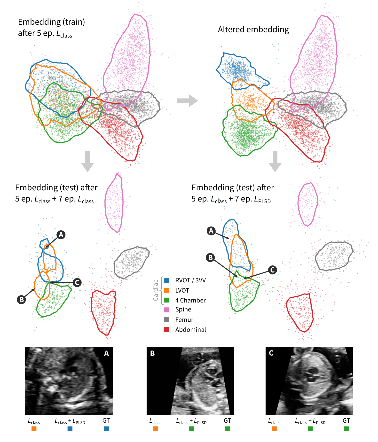
The ultrasound dataset is imbalanced, with 1,866 images in the three cardiac classes, and 2,911 images in the three non-cardiac classes. There are about twice as many 4CH images as RVOT/3VV, and three times as many 4CH images as LVOT. As a result, after five epochs of classification learning, our vanilla classifier could not properly distinguish between the three cardiac classes. This is apparent in the baseline embedding shown in Fig. 3 (top left).
We experimented with PLIs to improve the performance for the cardiac classes, in particular for RVOT/3VV and LVOT. Figure 3 (top right) shows the case of contracting and shifting the class clusters of RVOT/3VV and LVOT.
| RVOT* | 4CH | LVOT | Abd. | Femur | Spine | Cardiac | Other | ||
|---|---|---|---|---|---|---|---|---|---|
| Precision | Class. only | 0.82 | 0.82 | 0.42 | 0.93 | 0.98 | 0.97 | 0.77 | 0.96 |
| PLIs | 0.78 | 0.85 | 0.61 | 0.91 | 0.97 | 0.96 | 0.80 | 0.95 | |
| Recall | Class. only | 0.38 | 0.94 | 0.46 | 0.96 | 0.97 | 0.94 | 0.76 | 0.96 |
| PLIs | 0.73 | 0.94 | 0.28 | 0.96 | 0.97 | 0.94 | 0.81 | 0.96 | |
| -score | Class. only | 0.56 | 0.88 | 0.44 | 0.95 | 0.97 | 0.95 | 0.75 | 0.96 |
| PLIs | 0.76 | 0.89 | 0.41 | 0.94 | 0.97 | 0.95 | 0.80 | 0.95 |
After the latent interventions, training was resumed for 7 epochs with the mixed loss function defined in Eq. 1. We experimented with different values for ; all results given in this section are for , which was found to be a suitable value in this application scenario. For a fair comparison, training of the baseline network was also resumed for 7 epochs with pure classification loss. In both cases, the remaining training epochs were performed without data augmentation, but with all other hyperparameters kept the same as for the vanilla classifier.
The outputs were then embedded with the parametric -SNE learned on the baseline outputs (see Fig. 3, centre). By resuming the training with included embedding loss, the clusters for the three cardiac classes assume relative positions that are closer to those in the altered embedding. The contraction constraint also led to more convex clusters for the test outputs. Figure 3 (bottom) shows three exemplary images that were misclassified in case of the pure classification loss model, but correctly classified after applying PLIs. Further inspection showed that most of the images that were correctly classified after PLIs (but not before) had originally been embedded close to decision boundaries.
Table 1 lists the class-specific precision, recall, and -scores for the two different networks. By applying PLIs, the average quality for the cardiac classes could be improved without negatively affecting the performance for the remaining classes. In some experiments, we observed much larger quality improvements for individual classes. For example, in one case the -score for LVOT improved by a factor of two. In these extreme cases, however, local improvements were often accompanied by significant performance drops for other classes.
4 Discussion
The insights gained from PLIs about the relationship between a classifier and its latent space are based on an assessment of the model’s response to the interventions. This response can be evaluated on two axes: the embedding response and the performance response.
Simple classifications tasks, for which the baseline classifier already works well (e.g., MNIST) often show a considerable embedding response with only a minor performance response. This means that the desired alterations of the latent space are well reflected after retraining without strong effects on the classification performance. Such classifiers are flexible enough to accommodate the latent manipulations, likely because they are overparameterised. In more complex cases, such as CIFAR, the embedding response is weaker, but often accompanied by a more pronounced class-specific performance increase. For these cases, the learned representation seems to be more rigidly connected with the classification performance. Finally, the standard plane detection experiments showed that sometimes a minimal change in the embedding is accompanied by a considerable performance increase for the targeted classes. Here, the overall structure of the embedding seems to be fixed, but the classification accuracy can be redistributed between classes by injecting additional domain knowledge while allowing non-targeted classes to move freely.
In general, we found that too severe alterations of the latent space cannot be preserved well since the embeddings are based on local information. Furthermore, seemingly obvious changes made in the embedding may contradict the original classification task due to the non-linearity of the embedding. The strength of PLIs is that a co-evaluation of the two components of the loss function can reveal these discrepancies. As a result, even when PLIs cannot be used for improving a classifier’s performance, it can still lead to a better understanding of the flexibility of the model and/or the trustworthiness of the embedding.
In future work, we would like to experiment with parametric versions of different dimensionality reduction techniques and explore the potential of instance-level manipulations controlled via an interactive visualisation.
5 Conclusion
We introduced Projective Latent Interventions, a promising technique to inject additional information into neural network classifiers by means of constraints derived from manual interventions in the embedded latent space. PLIs can help to get a better understanding of the relationship between the latent space and a classifier’s performance. We applied PLIs successfully to obtain a targeted improvement in standard plane classification for ultrasound images without negatively affecting the overall performance.
Acknowledgments: This work was supported by the State of Upper Austria (Human-Interpretable Machine Learning) and the Austrian Federal Ministry of Education, Science and Research via the Linz Institute of Technology (LIT-2019-7-SEE-117), and by the Wellcome Trust (IEH 102431 and EPSRC EP/S013687/1.).
References
- [1] Baumgartner, C.F., Kamnitsas, K., Matthew, J., Fletcher, T.P., Smith, S., Koch, L.M., Kainz, B., Rueckert, D.: Sononet: real-time detection and localisation of fetal standard scan planes in freehand ultrasound. IEEE transactions on medical imaging 36(11), 2204–2215 (2017). https://doi.org/10.1109/TMI.2017.2712367
- [2] Bellet, A., Habrard, A., Sebban, M.: A survey on metric learning for feature vectors and structured data. arXiv preprint arXiv:1306.6709 (2013)
- [3] Brent, R.P.: Algorithms for minimization without derivatives. Courier Corporation (2013)
- [4] Chen, X., Weng, J., Lu, W., Xu, J., Weng, J.: Deep manifold learning combined with convolutional neural networks for action recognition. IEEE transactions on neural networks and learning systems 29(9), 3938–3952 (2017), 10.1109/TNNLS.2017.2740318
- [5] Dong, W., Moses, C., Li, K.: Efficient k-nearest neighbor graph construction for generic similarity measures. In: Proceedings of the 20th international conference on World wide web. pp. 577–586 (2011), https://www.cs.princeton.edu/cass/papers/www11.pdf
- [6] Erhan, D., Bengio, Y., Courville, A., Manzagol, P.A., Vincent, P., Bengio, S.: Why Does Unsupervised Pre-training Help Deep Learning? Journal of Machine Learning Research 11, 625–660 (2010), http://jmlr.org/papers/volume11/erhan10a/erhan10a.pdf
- [7] Krizhevsky, A., Nair, V., Hinton, G.: Cifar-10 (canadian institute for advanced research), http://www.cs.toronto.edu/˜kriz/cifar.html, accessed: 2020-03-16
- [8] Kulis, B., et al.: Metric learning: A survey. Foundations and trends in machine learning 5(4), 287–364 (2012)
- [9] LeCun, Y., Cortes, C.: The MNIST database of handwritten digits (2005), http://yann.lecun.com/exdb/mnist/, acessed: 2020-03-16
- [10] Lee, C.Y., Xie, S., Gallagher, P., Zhang, Z., Tu, Z.: Deeply-supervised nets. In: Artificial intelligence and statistics. pp. 562–570 (2015), proceedings.mlr.press/v38/lee15a.pdf
- [11] van der Maaten, L.: Learning a parametric embedding by preserving local structure. In: Artificial Intelligence and Statistics. pp. 384–391 (2009), http://proceedings.mlr.press/v5/maaten09a.html
- [12] van der Maaten, L., Hinton, G.: Visualizing Data using t-SNE. Journal of Machine Learning Research 9(Nov), 2579–2605 (2008), https://lvdmaaten.github.io/publications/papers/JMLR˙2008.pdf
- [13] McInnes, L., Healy, J., Melville, J.: UMAP: Uniform Manifold Approximation and Projection for Dimension Reduction. arXiv:1802.03426 (Dec 2018), http://arxiv.org/abs/1802.03426
- [14] Mead, A.: Review of the development of multidimensional scaling methods. Journal of the Royal Statistical Society: Series D (The Statistician) 41(1), 27–39 (1992). https://doi.org/10.2307/2348634
- [15] Min, M.R., van der Maaten, L., Yuan, Z., Bonner, A.J., Zhang, Z.: Deep supervised t-distributed embedding. In: Proceedings of the 27th International Conference on Machine Learning (ICML-10) (2010), https://www.cs.toronto.edu/˜cuty/DSTEM.pdf
- [16] NHS: Fetal anomaly screening programme: programme handbook June 2015. Public Health England (2015)
- [17] Poličar, P.G., Stražar, M., Zupan, B.: openTSNE: a modular Python library for t-SNE dimensionality reduction and embedding. bioRxiv (Aug 2019). https://doi.org/10.1101/731877, http://biorxiv.org/lookup/doi/10.1101/731877
- [18] Rauber, P.E., Fadel, S.G., Falcão, A.X., Telea, A.C.: Visualizing the Hidden Activity of Artificial Neural Networks. IEEE Transactions on Visualization and Computer Graphics 23(1), 101–110 (Jan 2017). https://doi.org/10.1109/TVCG.2016.2598838
- [19] Rusu, A.A., Rao, D., Sygnowski, J., Vinyals, O., Pascanu, R., Osindero, S., Hadsell, R.: Meta-learning with latent embedding optimization. arXiv:1807.05960 (2018), https://arxiv.org/abs/1807.05960
- [20] Tenenbaum, J.B.: A Global Geometric Framework for Nonlinear Dimensionality Reduction. Science 290(5500), 2319–2323 (Dec 2000). https://doi.org/10.1126/science.290.5500.2319, http://www.sciencemag.org/cgi/doi/10.1126/science.290.5500.2319
- [21] Tomar, V.S., Rose, R.C.: Manifold regularized deep neural networks. In: Fifteenth Annual Conference of the International Speech Communication Association (2014)
- [22] Wold, S., Esbensen, K., Geladi, P.: Principal component analysis. Chemometrics and intelligent laboratory systems 2(1–3), 37–52 (1987). https://doi.org/10.1016/0169-7439(87)80084-9