Spin Hall effect in heavy ion collisions

The study of spin current, the flow of spin, has triggered intense research. The generation of spin current is a key concept in the field of spintronics Žutić and Dery 2011, and can be employed to probe intriguing properties of quantum materials Han et al. 2019. One prominent mechanism of the generation of spin current is spin Hall effect (SHE) Sinova et al. 2015, by which an electric field will induce a transverse spin current perpendicular to the direction of the electric field. SHE has been observed in a number of table-top experiments Kane and Mele 2005; Wunderlich et al. 2005; Sinova et al. 2015.

When the temperature and/or density gradient is non-zero, they could induce analogous spin Hall current. The resulting spin polarization distribution function of fermions (anti-fermion) $\vec{\mathcal{P}}_{+}$ ($\vec{\mathcal{P}}_{-}$), in the rest frame of the fluid, can be written as:

where $\vec{p}$ denotes the spatial momentum. Here, $\sigma^{T,\mu}_{\pm}$ depends on temperature $T$ and chemical potential $\mu$ as well as the energy of fermion $\varepsilon_{\vec{p}}=\sqrt{\vec{p}^{2}+m^{2}}$ where $m$ is the fermion mass. In Eq. (1), thermodynamic force, collectively denoted by $\vec{F}={\vec{\partial}}T,T{\vec{\partial}}(\mu/T)$, plays the role of analogous electric field. We shall refer Eq. (1) as the “thermally-induced spin Hall effect” (TSHE). The first term in Eq. (1), i.e. spin Hall current induced by temperature gradient, is also known as the spin Nernst effect (SNE), and has been observed in platinum Meyer et al. 2016 and in W/CoFeB/MgO heterostructures Sheng et al. 2017 a few years ago.

In this work, we shall study TSHE (1) in hot and dense nuclear matter created in heavy-ion collisions. The spin polarization induced by vorticity $\vec{\omega}$ and magnetic field in heavy-ion collisions has attracted much experimental Adamczyk et al. 2017a; Niida 2019; Adam et al. 2018; Adam et al. 2019; Acharya et al. 2020; Acharya et al. 2019; Zhou 2019 and theoretical efforts Gao et al. 2012; Becattini et al. 2013; Fang et al. 2016; Pang et al. 2016; Becattini and Karpenko 2018; Florkowski et al. 2019; Liu et al. 2019; Weickgenannt et al. 2020; Fu et al. 2021 (see Refs. Kharzeev et al. 2016; Bzdak et al. 2020; Becattini and Lisa 2020; Gao et al. 2020 for reviews). TSHE is different from the generation of spin polarization induced by fluid vorticity $\vec{\omega}$. To see such difference, let us assume for the sake of discussion, that $\sigma^{T,\mu}$ only depends on $p=|\vec{p}|$. We then have from Eq. (1), $\int_{\vec{p}}\mathcal{P}^{{\rm SHE}}=0$, meaning TSHE does not generate net polarization after the average over the momentum. In Ref. D’Yakonov and Perel’ 1971 where the notion of spin current is originally introduced, spin current is described by a tensor ${\cal S}^{ij}$. The first index of ${\cal S}^{ij}$ indicates the direction of flow, while the second one indicates which component of the spin is flowing, i.e., ${\cal S}^{ij}\propto\int_{\vec{p}}p^{i}\mathcal{P}^{j}$. Eq. (1) then implies $S^{ij}\propto\epsilon^{ijk}\,F_{k}$, the generation of spin current. In contrast, in the same setting, turning on a vorticity will simply induce a net polarization $\propto\vec{\omega}$, but will not induce spin current $S^{ij}$. Therefore, the study of TSHE complements the existing work on the vorticity effects.

This work is organized as follows. To quantify induced spin Hall current, we determine $\sigma^{T}_{\pm},\sigma^{\mu}_{\pm}$ by evaluating the relevant correlation functions based on the linear response theory in Sec. II, see Eqs. (22), (23) for explicitly expression. In Sec. III, we then estimate the magnitude of observables associated with local spin polarization due to TSHE at two representative beam energies, namely $\sqrt{s}_{NN}=200$ GeV and $\sqrt{s}_{NN}=19.6$ GeV, and will focus on central collisions. It is well-known that the effects of temperature gradient and fluid vorticity in combination as the “thermal vorticity” will induce a specific pattern in the azimuthal angle dependence of $P^{i}(\phi)$ non-central collisions Pang et al. 2016; Becattini and Piccinini 2008; Becattini et al. 2008; Becattini et al. 2013; Wu et al. 2019 (see Ref. Becattini 2020 for a review). However, the analysis of local spin polarization in central collisions has attracted much less attention. We summarize our results in Sec. IV

In this section, we explain in detail on how to determine $\sigma^{T,\mu}_{\pm}$ which quantify TSHE by evaluating the relevant correlation functions. The method used here is similar to the one developed by Luttinger in Ref. Luttinger 1964 to derive Kubo formula for thermal conductivity. Below, we consider the simplest case when there is only one species of fermions (anti-fermions) with one unit of $U(1)$ charge throughout, although relaxing this simplification is straightforward. We have also assumed that fermionic constituents of the systems are weakly coupled so that we can obtain those correlation functions from an one-loop thermal field calculation.

Let us begin with the operator:

where $\gamma^{5},\gamma^{i}$ denote the standard gamma matrices. At this point, $\psi$ represents a generic Dirac field. According to the quantum field theory, the phase space distribution of spin polarization is given by the Wigner transform:

with $\langle\ldots\rangle$ denoting the thermal ensemble average. Here $\vec{\mathcal{P}}$ include contribution from both particles and anti-particles.

We shall consider a medium that is initially in equilibrium and is isotropic, and hence at this point, $\vec{\mathcal{P}}=0$. We next turn on an electric field and a non-flat metric

where $\eta_{\mu\nu}$ is the flat-space metric. Such external fields will in turn induce temperature and chemical potential gradient. ${\vec{\mathcal{P}}}$ arises due to the nonuniformity of the system and should be expressible in terms of a gradient expansion as

where $\sigma^{T,\phi,\mu,E}_{\pm}$ would depend on $T,\mu$ and $p$. Here, it is not necessary to include the acceleration of the velocity field $\partial_{t}\bm{v}$ which can be expressed as a specific linear combination of gradient terms shown in Eq. (5) using the ideal hydrodynamic equations.

Following Ref. Luttinger 1964, we then consider the behavior of constitutive relation Eq. (5) in two different limits: a) The “ rapid” case, where the typical frequency is much larger than gradient b) the “slow” case, in which the typical gradient is much larger than frequency. In the “rapid” case, the system does not have time to adjust to generate temperature and chemical potential gradient even if the external fields are present, so we have

In the opposite limit, the system will reach hydrostatic state, in which $\vec{E}=T\nabla(\mu/T)$ and $T^{-1}{\vec{\partial}}T={\vec{\partial}}\phi$, and hence we have:

Taking the difference between (7) and (6), we obtain

Based on Eq. (8), we can extract $\sigma^{T,\mu}_{\pm}$ from the relevant retarded correlation functions:

where $\hat{J}^{0}=\bar{\psi}\gamma^{0}\psi$ and $\hat{T}^{\mu\nu}$ denotes the stress-energy tensor. Introducing Fourier transform with $q_{0},\vec{q}$ being frequency and momentum conjugate to $t,\vec{x}$ respectively, we have

In what follows, we shall first evaluate $G$ at one loop, and then extract $\sigma^{T,\mu}_{\pm}$ by comparing Eq. (11) with Eqs. (8).

At one loop order (see Fig. 2), $G^{i}(\tilde{\omega}_{n},\vec{q};\vec{p})$ as a function of the Bosonic Matsubara frequency $\tilde{\omega}_{n}=2n\pi T$ is given by

where $\vec{p}_{1}=\vec{p}+\frac{\vec{q}}{2},\vec{p}_{2}=\vec{p}-\frac{\vec{q}}{2}$. Here the Euclidean propagator as function of the Fermionic Matsubara frequency $\nu_{n}=\pi T(2n+1)+\mu$ and momentum $\vec{p}$ reads

with $\Lambda_{s}(\vec{p})=s\gamma^{0}\varepsilon_{\vec{p}}-\vec{p}\cdot\bm{\gamma}+m$, and

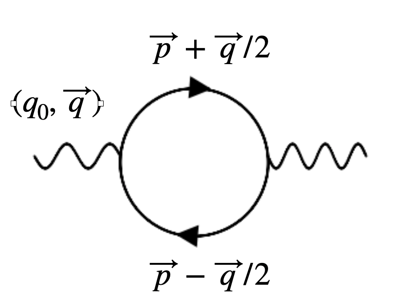
To evaluate Eq. (12), we first take the trace:

If one were computing the response of axial current $\vec{j}_{5}=\int d^{3}\vec{p}/(2\pi)^{3}\vec{\mathcal{P}}$ to external disturbance by loop diagrams, one has to integrate out momentum in the loop (e.g. Ref. Lin and Yang 2018). However, since we are interested in $\vec{\mathcal{P}}$, we only need to use the book-keeping formula to perform the summation over the Matsubara frequency:

where $\varepsilon_{1,2}=\varepsilon_{\vec{p}_{1,2}}$. Here, $n_{\pm}(\varepsilon)=1/(e^{(\varepsilon\mp\mu)/T}+1)$ are Fermi-Dirac distribution for fermion($+$) and anti-fermion ($-$). By substituting Eq. (15) and Eq. (16) into Eq. (12), and perform the analytic continuation, which amounts to replace $\tilde{\omega}_{m}$ with $q_{0}+i0^{+}$, we obtain the desired expression

Here,we have used $\varepsilon_{1}-\varepsilon_{2}=\bm{v}_{\vec{p}}\cdot\vec{q},n_{\pm}(\varepsilon_{1})-n_{\pm}(\varepsilon_{2})=(\partial n_{\pm}(\varepsilon_{\vec{p}})/\partial\varepsilon_{\vec{p}})\bm{v}_{\vec{p}}\cdot\vec{q}$ by assuming $q_{0},q\ll\varepsilon_{\vec{p}}\sim T,\mu$. In another word, we have expanded $G^{i}$ to the first non-trivial order in $q_{0}/\varepsilon_{\vec{p}},q/\varepsilon_{\vec{p}}$ to obtain (17).

At one loop order the expression for $G^{i,00}$ is given by replacing $\gamma^{0}$ in Eq. (12) with $\gamma^{0}i\nu_{m}$. Hence the evaluation of $G^{i,00}$ becomes a trivial extension of the calculation of $G^{i}$, yield

We now extract the induced fermion (anti-fermion) local spin polarization $\vec{\mathcal{P}}_{+}$ ($\vec{\mathcal{P}}_{-}$) by substituting Eq. (17) Eq. (21) into Eq. (11). We assume that $\mathcal{P}_{+}$ ($\mathcal{P}_{-}$) should depend on $n_{+}$ ($n_{-}$) and/or the derivative $\partial n_{+}/\partial\varepsilon_{\vec{p}}$ ($\partial n_{-}/\partial\varepsilon_{\vec{p}}$) only, and require $\vec{\mathcal{P}}(\vec{p})=\vec{\mathcal{P}}_{+}(\vec{p})+\vec{\mathcal{P}}_{-}(-\vec{p})$. Use the prescription outlined above, we obtain

where we have used $\vec{E}=-i\vec{q}A_{0}$ and where

The cautious reader might worry if one could do such separation when fermion and anti-fermion are mixed with each in the presence of an external field. However, since we consider fermions with energy $\varepsilon_{\vec{p}}\gg|\vec{q}|,q_{0}$, they will interact with anti-fermions of approximately the same energy $\varepsilon_{\vec{p}}$, meaning the relative phase between the fermions and anti-fermions participated in such interaction is approximately $2\varepsilon_{\vec{p}}\Delta t$ for a given duration $\Delta t$. Therefore one should be able to integrate out fast oscillating anti-fermions in the long time limit and hence obtain distribution for fermions. One can draw a parallel conclusion for anti-fermions. See Refs. Son and Yamamoto 2013; Manuel and Torres-Rincon 2014; Manuel et al. 2016 for explicit examples on obtaining particle/anti-particle distribution through such integrating-out procedure.

We now return to the extraction of $\sigma^{T,\mu}_{\pm}$. Comparing Eq. (5) in Fourier space with Eqs. (8) and using $\lim_{r}=\lim_{q_{0}\to 0}\lim_{\vec{q}\to 0}$ and $\lim_{s}=\lim_{\vec{q}\to 0}\lim_{q_{0}\to 0}$, we find

Note $\sigma^{T}_{+},\sigma^{\mu}_{+}<0$. In the massless limit, the expression of $\sigma^{\mu}$ in Eq. (22) agrees with that obtained in Ref. Hidaka et al. 2017 using chiral kinetic theory. This $\mu$-gradient induced spin polarization has also been obtained for a Landau fermion liquid with chiral fermions from quantum kinetic theory in Ref. Son and Yamamoto 2013 (see also Refs. Hidaka et al. 2017; Hattori et al. 2019; Fang et al. 2016. For related studies, see for example Refs. Pu et al. 2015; Sheng et al. 2020). Our main results in this section, Eqs. (22), (23) apply to fermions with arbitrary mass in a system with generic $\mu,T$.

The authors of Refs. Becattini and Piccinini 2008; Becattini et al. 2008; Becattini et al. 2013 consider a class of hydrodynamic profile which satisfies the so-called ”equilibrium/static” condition Becattini 2012; Becattini et al. 2019, i.e.,

and find that the spin polarization is proportional to the thermal vorticity

The thermal vorticity effects as defined in Eq. (25) include the contribution from both fluid vorticity (the anti-symmetric part of the flow velocity gradient) and temperature gradient. Note, the thermal vorticity also contains a term proportional to the acceleration $u^{\mu}\partial_{\mu}u^{\nu}$, but this term can be replaced by temperature gradient if one combines ideal hydrodynamic equation with the condition (24). However, the effect of $\mu/T$ gradient is different from that of thermal vorticity since the condtion (24) requires the homogeneity of $\mu/T$, meaning the analysis assuming such condition does not account for the contribution from $\mu/T$ gradient.

It is worth pointing out that the effects of different hydrodynamic gradients on spin polarization have to be extracted from different correlation functions. As we have just derived in this Section, the effects of $\mu$ and temperature gradient can be extracted from correlator $G^{i}$ (17) and $G^{i,00}$ (21) respectively. In Ref. Liu and Yin 2021, we further show how to determine the fluid vorticity effect from $G^{i,0j}\equiv i\langle\mathcal{P}^{i}(t,\vec{x})\,T^{0j}(0,0)\rangle\theta(t)$ ¹¹ 1 As shown in later works. Liu and Yin 2021; Fu et al. 2021; Becattini et al. 2021, shear tensor (the symmetric part of flow gradient) could also induce spin polarization in a specific way. . Since the physical content of those correlators are not identical, we expect that those effects may generally tell us complimentary information on the spin physics of a medium.

In this work, we investigate the perspective of detecting spin Hall current induced by temperature and chemical potential gradient, i.e., thermally-induced spin Hall effect (TSHE), in fireballs created in heavy-ion collisions. We use linear response theory to derive those effects. Complementary to the measurement of spin polarization induced by vorticity, the exploration of spin Hall current will provide a new probe to the quantum transport phenomenon of QCD matter. We demonstrate that the induced spin Hall current would manifest itself through the azimuthal angle dependence of the local spin polarization of $\Lambda$ and $\bar{\Lambda}$, $P^{i}(\phi_{p})$, yielding a qualitative distinctive signature. We propose to use the first Fourier harmonics of $P^{i}(\phi_{p})$, “directed spin flow”, to quantify spin Hall current. We estimate the magnitude of “directed spin flow” is of the order $10^{-4}-10^{-3}$, and show it can be very sensitive to the rapidity.

We have made simplifications at many points, particularly on the parametrization of density and flow profile on the freeze-out surface, for illustrative purposes. We have limited ourselves to the discussion of spin current induced by longitudinal $\mu_{B}$ and/or $T$ gradient, but the presence of gradient in the transverse plane could lead to possible observable effects as well. Therefore future studies based on state of the art hydrodynamic modeling Shen 2020 are desirable. As far as background contribution is concerned, we note when the spin polarization induced by some specific local vorticity profile is boosted by the bulk flow, it might contribute to “directed spin flow” observables, see for example Ref Xia et al. 2018. We point out however the direction of spin Hall current induced by the gradient of $\mu_{B}$ would be opposite between $\Lambda$ and $\bar{\Lambda}$, and this property might be employed to distinguish the signal from background contribution.