A Step Towards Interpretable
Authorship Verification
Abstract
A central problem that has been researched for many years in the field of digital text forensics is the question whether two documents were written by the same author. Authorship verification (AV) is a research branch in this field that deals with this question. Over the years, research activities in the context of AV have steadily increased, which has led to a variety of approaches trying to solve this problem. Many of these approaches, however, make use of features that are related to or influenced by the topic of the documents. Therefore, it may accidentally happen that their verification results are based not on the writing style (the actual focus of AV), but on the topic of the documents. To address this problem, we propose an alternative AV approach that considers only topic-agnostic features in its classification decision. In addition, we present a post-hoc interpretation method that allows to understand which particular features have contributed to the prediction of the proposed AV method. To evaluate the performance of our AV method, we compared it with ten competing baselines (including the current state of the art) on four challenging data sets. The results show that our approach outperforms all baselines in two cases (with a maximum accuracy of 84%), while in the other two cases it performs close to the strongest baseline.
Keywords: Authorship verification Topic-Agnostic Features Interpretation.
1 Introduction
With the constant increase of documents worldwide, more and more possibilities of identity misuse are becoming established. One example of such identity abuse is “CEO Fraud” – a sophisticated email scam – in which an attacker sends an email to an employee on behalf of a CEO to perform a specific action (e. g., transferring money or sending confidential company information). Another form of identity abuse occurs in the context of compromised accounts, where the attacker distributes messages in the name of the victim. In addition, identity abuse can occur in fake reviews in which, for example, an attempt is made on behalf of an alleged person to positively advertise a product or service provider. One countermeasure that can be applied in all these scenarios is to compare the writing style of the questioned documents to the writing style of those documents, of which the true author is known. By this, the question can be answered (with a certain degree of probability) whether the unknown document was also written by . The comparison of documents based on their writing style is particularly relevant if no other metadata are available to clarify the identity of the unknown author.
Authorship verification (AV) – a branch of research in digital text forensics – has been dealing with this question for over two decades. Technically, AV represents a similarity detection problem, where for an unknown document and a known document it has to be determined whether both were written by the same author . Here, the focus of the similarity determination lies on the writing style of the documents and not on other factors such as the topic or genre. Otherwise, if and have the same topic but were written by two different authors, an AV method would clearly miss its intended goal. A large number of existing AV methods including [8, 10, 29, 32, 35, 37] make use of character -grams (overlapping character sequences), which are known to be closely associated to particular content words and, therefore, can be problematic when dealing with authorship [27]. Style analysis, however, must abstract from content and focus on content-independent formal properties of linguistic expressions in a text [14]. In the light of this conclusion, we propose an alternative approach which, by design, considers only such text units that reflect valid stylistic markers. Our contribution in this paper is threefold: First, we propose a number of topic-agnostic feature categories that effectively quantify the writing style of documents. Second, we propose a transparent AV method that can be applied to challenging AV tasks. These include cases, where and consist of only a few sentences or cases, in which both documents differ thematically. Third, we propose a post-hoc interpretation method, which allows to understand which features contributed to the prediction of our AV method.
The remainder of the paper is organized as follows. Section 2 discusses previous work in the context of AV. In Section 3, we propose a number of feature categories, which will be used by our AV method introduced in Section 4. In Section 5, we then describe our post-hoc interpretation method. Afterwards, we present our experimental evaluation in Section 6 and, finally, in Section 7 we conclude the work and provide ideas for future work.
2 Previous Work
The core of every AV method is a classification model that aims to decide whether a questioned document was written by a certain author , for which a set of reference documents is given. With regard to their classification models, we have identified three categories of AV methods in our previous research work [17], which are summarized below.
The first category are unary AV methods that determine their classification model solely on the basis of . A unary AV method assumes to be written by , if it is stylistically similar to the documents in . The second category are binary-intrinsic AV methods that determine their classification model on the basis of a given training corpus. This corpus consists of a number of verification cases with a ground truth of the form Y (same-author) and N (different-author). A binary-intrinsic AV method treats the unknown and known documents as a single unit (for example, a feature vector). If is more similar to the Y-cases, the method accepts as the author of . If, on the other hand, is more similar to the N-cases, is assumed to be written by another author. In any case, the decision is made solely the basis of and the learned model (hence, intrinsic). The third category are binary-extrinsic AV methods that determine their classification model on the basis of external (so-called impostor [29]) documents which, for example, are gathered by using a search engine. In this context, the documents in represent samples of the class Y, while the impostor documents act as samples of the counter class N. A binary-extrinsic AV method assumes to be written by , if it is stylistically similar to the documents in . Otherwise, is rejected as the true author, if is more similar to the impostor documents. Over the last two decades, numerous AV approaches have been proposed that can be assigned to one of these three categories.
A recently published unary AV approach, which we refer to as AVIF, was developed by Neal et al. [32] for the purpose of continuous verification. Their method is based on an isolation forest classifier, which, like many other AV methods, considers character -grams as underlying features. AVIF yielded a high recognition accuracy using very small training samples of 50 and 100-character blocks. However, in their study the authors explain that the method was only evaluated on positive samples (in other words, instances of the Y-class). Therefore, it is not clear how well AVIF performs under realistic conditions in which both classes (Y and N) exist.
A common binary-intrinsic AV approach, which we denote by the name ProfAV, was proposed by Potha and Stamatatos [34]. Their method considers two documents and as character -gram profiles and measures their relative differences using a predefined dissimilarity function. If the resulting dissimilarity score exceeds a certain threshold (derived from the distribution of Y/N-samples in a given training corpus), is assumed to be written by . Potha and Stamatatos [34] demonstrated that ProfAV was able to outperform every single AV method submitted to the first AV-competition as a part of the PAN shared tasks [22].
One of the most influential and successful binary-extrinsic AV approach is the Impostors Method (IM) proposed by Koppel and Winter [29], which laid the foundations for many subsequent AV approaches (for example, [39, 23, 24, 25, 35]). IM can be broken down into two steps. In the first step, appropriate impostor documents have to be collected according to a predefined strategy (e. g., using a search engine or a static corpus with suitable documents). In the second step, a feature randomization technique is applied iteratively to measure the similarity between pairs of documents. If, given this measure, a suspect is picked out from among the impostor set with sufficient salience, then the suspect is assumed to be the author of [29]. Two variants of IM, namely ASGALF proposed by Khonji and Iraqi [23] and GenIM proposed by Seidman [39] were the best-performing approaches in the first and second PAN-AV competitions [22, 41]. An alternative binary-extrinsic AV approach is the NNCD method proposed by Veenman and Li [45]. In contrast to IM, their method delegates the entire feature engineering procedure to a state of the art compression-algorithm. Here, is assumed to be written by if the compressed version of is dissimilar to the compressed version of the impostor documents. Both NNCD [45] and GenIM [39] were the best performing approaches in the first PAN-AV competition [22].
3 Feature Categories
In this section, we propose a number of feature categories that are used by our AV approach to capture the writing style of documents. A part of these derive from certain feature categories used in previous studies. The remaining feature categories, however, have been not considered so far in the context of AV, at least to our best knowledge. All feature categories are summarized in Table 1 along with a number of examples. In the following subsections, we first introduce all feature categories in detail. Afterwards, we explain which design decisions we made in regard to their hyperparameters. Finally, we describe the scope from where all proposed features are extracted and how we normalized them.
| ID | Feature category | Range | Sample | Sample output |
| Punctuation -grams | ||||
| TA sentence and clause starters | — | |||
| TA sentence endings | — | |||
| TA token -grams | ||||
| TA masked token -grams |
3.1 Topic-Agnostic Words and Phrases
Function words can be seen as the most common choice in the field of authorship analysis, when it comes to select topic-agnostic features. However, in the literature it often remains unclear what is exactly understood and represented under the term “function words”. In many existing studies (for example, [11, 21, 47]) no detailed explanation is provided regarding the question, which specific function word categories (or at least which specific words) were taken into account. Another peculiarity that can be seen in the literature, is the varying number of considered function words. For example, Chandrasekaran [11], Binongo [7], Srinivasa [38] and Zhao and Zobel [46] make use of 24, 50, 150 and 365 function words, respectively. In view of these different numbers, the question arises why only individual subsets are considered rather than using the entire spectrum of function words. Instead of making use of non-structured and incomplete lists, Varela et al. [44] and Pavelec et al. [33] follow a different approach, in which they consider subcategories of function words such as pronouns, conjunctions, subclasses of adverbs and other word forms. By this, a better insight can be gained regarding the question which specific type of function words were actually taken into account.
Motivated by this idea, we opted for a similar but more systematic approach, in which we consider all existing categories of function words along with other carefully selected topic-agnostic (hereafter, abbreviated as TA) categories. First, we assemble a comprehensive list consisting of words and phrases that belong to these categories (cf. Table 2). Based on , we then derive different TA feature categories (described below) that can be used to model the writing style of documents across different linguistic layers. For the construction of , we use a variety of words and phrases classified into 20 categories including function words, empty verbs, contractions, generic adverbs as well as transitional words and phrases. All considered words and phrases, which are known in the literature [33, 7, 43] to be content and topic independent, have been collected from different sources, in particular, linguistic books and stylometry papers. The transitional phrases cover a number of categories including causation, contrast, similarity, clarification, conclusion, purpose and summary. With regard to the verbs, we take the respective tenses11 1 To generate the tenses, we used the pattern framework [13] available at https://github.com/clips/pattern. into account (for example, give ) in order to enrich . All categories of words and phrases contained in are summarized in Table 2 along with a number of examples.
| Category | Examples |
| Conjunctions | |
| Determiners | |
| Prepositions | |
| Pronouns | |
| Quantifiers | |
| Auxiliary verbs | |
| Delexicalised verbs | |
| Empty verbs | |
| Helping verbs | |
| Contractions | |
| Adverbs of degree | |
| Adverbs of frequency | |
| Adverbs of place | |
| Adverbs of time | |
| Pronominal adverbs | |
| Focusing adverbs | |
| Conjunctive adverbs | |
| Transition words | |
| Transitional phrases | |
| Phrasal prepositions |
Note that due to the ambiguities occurring in the English language, a number of function words appear in multiple categories. For example, "but" and "for" are both prepositions and conjunctions, whereas "few" represents a pronoun and a quantifier. However, regarding the features in , we do not differentiate between the different meanings of these homographs22 2 Homographs are words with the same spelling but different meaning.. Based on , we derive additional feature categories which are described in the following.
3.1.1 Punctuation -Grams
Punctuation marks represent syntactic features that quantify the grammatical structures an author uses and, thus, are content and topic independent [43]. As punctuation -grams we define a sequence of consecutive punctuation marks where letters, digits and other non-punctuation characters are skipped (cf. Table 1). Among others, punctuation -grams capture specific symbols that occur at word-internal level such as hyphens or apostrophes used in contractions (e. g., "we’ve" or "they’re"). Furthermore, they allow to recognize unusual punctuation habits reflecting the individual writing style of an author such as combinations of question and exclamation marks (e. g., "?!?" or "!?!"), which occur in informal documents. In total, we consider three punctuation -gram feature categories () that are not dependent on the list . However, the feature categories make use of (punctuation unigram).
3.1.2 TA Sentence and Clause Starters
Words or phrases that appear at the beginning of sentences or clauses can reflect one aspect of an author’s writing style. We therefore consider such sentences and clause starters as a distinct feature category. However, since our focus lies on TA-based features, we make sure that a word or phrase appearing at the beginning of a sentence or a clause is included in . Note that in case of clauses, we consider the preceding punctuation mark (comma or semicolon) together with the subsequent word or phrase as a whole feature (cf. Table 1).
3.1.3 TA Sentence Endings
Words or phrases that appear at the end of sentences might also reflect a stylistic habit of authors. We therefore consider such features as a distinct feature category and make sure (analogous to ) that they are included in .
3.1.4 TA Token -Grams
These feature categories can be seen as a form of standard token -grams with the restriction that each token in a token -gram represents either a punctuation or a word appearing in (cf. Table 1). Note that for , the respective feature category is essentially the list , which is obtained by merging all categories listed in Table 2.
3.1.5 TA Masked Token -Grams
These feature categories also represent a form of token -grams with the restriction that tokens in a token -gram are either punctuation marks or words appearing in . The remaining tokens, on the other hand, represent topic-related words, which are then masked by the non-punctuation character #. The intention behind these feature categories is to enable the detection of contexts surrounding or adjacent to topic-agnostic words (cf. Table 1).
3.2 Feature Category Ranges
In previous AV works (e. g., [34, 20, 8]) -gram-based feature categories have been treated as a single concept, where the most suitable was chosen on the basis of a hyperparameter optimization procedure. In contrast to this, we treat -gram-based feature categories independently so that, for example, punctuation - and -grams represent two individual feature categories. There is a simple justification for this decision: If we would restrict ourselves to only one specific , optimized on a training corpus, we might miss important features occurring in the unseen data (test corpus) that can only be captured with an alternative setting of . Allowing multiple settings of for the same feature category can, therefore, help to counteract a possible mismatch between training and test data.
In the following, we explain the considerations behind the ranges of the -gram-based feature categories listed in Table 1. For the punctuation -grams, we set as a lower limit which is useful in cases where sentences comprise only a single punctuation (e. g., full-stop, question or exclamation mark). As an upper limit, we set , as it can be expected that longer punctuation sequences between the unknown and known documents will be scarce (more on this in the next subsection). Regarding TA token -grams, we set and as a lower and upper limit, respectively. For the former, we aim to capture at least single words in the documents. Here, we expect that a part of these features will be present in both documents, in most of the cases. With regard to longer sequences, we aim to capture specific phrases that can be relevant for individual authors. However, sequences with more than four tokens are less likely to appear, especially between short documents so that can be seen as a good compromise. For the TA masked token -grams, we set as a lower limit, as one of our intentions is to capture (masked) topic words surrounded by topic-agnostic words, so that is a minimum limit. As an upper limit, we set for the same reason mentioned for TA token -grams.
3.3 Scope of Feature Extraction
In existing AV studies it is often not mentioned which scope is considered to extract -gram-based features. Here, the scope might be the entire text, paragraphs, sentences, clauses, phrases or tokens. Depending on the considered scope, the dimension of the generated feature space may vary which, in turn, may affect the verification results. For example, extracting token -grams from single sentences would result in a smaller number of features, in contrast to the extraction from the whole text. This is because token -grams cross sentence boundaries, so that respective cross-sentence features are not taken into account. Despite the smaller number of available features, we have decided, with regard to our AV approach, to extract all -gram-based features exclusively from the sentence-level of the documents. The reason for this is that in practice short text fragments (e. g., social media posts or email text bodies) are often concatenated to obtain a sufficient document length, so that one sentence might not always have a connection to a subsequent sentence. Hence, if we extract -gram-based features from the entire text, we would erroneously create artificial cross-sentence features that may not occur in texts of a particular author. Note that for feature extraction, we only consider lower case in order to capture all possible case variants (for example, "the", "The", "THE"), which can occur especially in informal texts.
4 Verification Method
In this section, we present our AV approach TAVeer33 3 TAVeer stands for “Topic-agnostic Authorship Verifier based on equal error rate”., which is inspired by the methodology of biometric recognition systems. These aim to recognize individuals, based on a variety of physiological characteristics and behavioral features obtained from e.g. the hand, vein, fingerprint, face, eye, ear or voice. Here, the equal error rate (EER) represents a statistic used to show biometric performance in the context of a verification task. Essentially, EER corresponds to a point on a ROC curve where the false acceptance rate is equal to the false rejection rate.
Given a questioned document and a document from a known author , the goal of our method is to determine whether was also written by . To achieve this goal, TAVeer employs an ensemble of distance-based classifiers, where each one aims to accept or reject the questioned authorship of . Each classifier is provided with a category of stylistic features extracted from an individual linguistic layer (in each document). In this context, EER serves as a thresholding mechanism, where erroneous verification predictions in either direction are treated equally. This is different from other AV methods. The approach of Bevendorff et al. [6], for example, heavily prioritize precision over recall.
TAVeer can essentially be divided into the two phases training and inference. In the training stage, a model has to be “learned” on the basis of a given training corpus . Here, each denotes a verification case, for which the ground truth (Y/N) is known beforehand. In the inference stage, the generated model is applied to an unseen verification case in order to accept or reject the questioned authorship. In what follows, we first describe the preliminaries for TAVeer and afterwards its two stages.
4.1 Preliminaries
Before describing our approach in detail, we first explain what exactly is considered as an input, how this input is represented and on which basic functionality it depends in order to measure the (dis)similarity between the documents.
4.1.1 Document Input
TAVeer follows the profile-based paradigm that, to our best knowledge, was first described by Potha and Stamatatos [34] in the context of AV. Given a set of reference documents for a known author , the idea behind the profile-based approach is to concatenate all documents in into a single document . Thus, a verification case is transformed from to , which represents the document input for TAVeer.
4.1.2 Document Representation
As a document representation technique, we consider a bag-of-features model, in which all involved features are treated independently from each other. Let be the proposed feature categories (cf. Table 1) and be the global set of documents. We define a function , which transforms and according to a given feature category to two real valued vectors, where denotes the dimension of the feature space spanned by the features from contained in the documents and . Consider for example as a feature category, which describes a set of punctuation marks "-", ";", "?", .... Applying to and yields all punctuation marks, that exist in at least one of the documents and adds them to a list . Then, two vectors and are created, where each and represents the absolute frequency of the corresponding punctuation mark in each document, respectively. As a final step, we normalize each vector by its Manhattan norm, denoted as , so that all contained features are scaled into the (real) interval and sum up to one. This procedure holds for all feature categories.
4.1.3 Distance Function
To measure the (dis)similarity between two generated feature vectors and , we use a distance function dist. For this, we have chosen the well-known Manhattan metric, defined by:
| (1) |
which has been used in a number of previous studies on stylometry (for example, [9, 2]). The Manhattan metric benefits from its simplicity and also from the fact that it allows easy interpretation of which specific features have contributed to the verification result (as will be shown in Section 6.4.2).
4.2 Model Learning
Given the training corpus and the set of all considered feature categories , the objective of this step is to construct a model , which represents the optimal combination of feature categories obtained on . In the following, we describe the necessary sub-steps to create .
4.2.1 Computing Thresholds
In this sub-step, the individual thresholds have to be computed for the feature categories. Using Equation 1, we calculate for each verification case and each feature category the respective distance . As a thresholding technique, we select the equal error rate (EER), which describes the point, where the false positives rate is equal to the false negatives rate. Since all corpora used in our experimental setting are balanced, a threshold, which will result in an EER, can be obtained by calculating the median of the distances over all cases in the corpus. Consequently, for all feature categories, we obtain the corresponding thresholds as follows:
| (2) |
Note that in case where an exact EER is not feasible (for example, when multiple distance values are equal) the median provides the closest approximation of the EER.
4.2.2 Similarity Function
The introduced distance function (cf. Equation 1) allows us to compute distances between pairs of feature vectors. However, the resulting distances are not calibrated with respect to the individual thresholds from the previous sub-step. Therefore, we designed a similarity function sim that considers as an input a distance , a threshold and the upper bound of the provided distance function (in our case, the Manhattan metric). Recall that in the context of our approach, all feature vectors are normalized using the Manhattan norm . Consequently, all features in each vector sum up to 1. Based on this fact, the lower and upper bound of dist can be calculated by
such that holds. An important requirement regarding our similarity function is that the resulting score is calibrated in a way that 0.5 represents the decision boundary. One possible definition for a function sim that transforms a distance into the range and simultaneously calibrates the resulting similarity score with respect to this “natural” decision boundary is:
| (3) |
Figure 1 illustrates the behavior of sim with respect to the lower and upper bound of the Manhattan metric.
Note that by considering as a variable parameter, we can easily substitute the Manhattan metric with any other distance function, as long as its respective upper bound is known. Furthermore, it should be highlighted that any other definition for sim that also fulfills the same requirement can be used instead.
4.2.3 Classification Function
The similarity function sim from the previous sub-step can calculate a calibrated similarity value for a given distance and a threshold for a single feature category. However, the idea behind TAVeer is to determine whether a questioned authorship between two documents holds based on multiple feature categories. Let denote a set, which comprises pairs of feature categories and their associated thresholds and the power set (without the empty set) holding all possible combinations of these pairs. We denote a single by the term ensemble. Furthermore, we denote an ensemble comprising a single pair as an atomic ensemble. To compute a similarity value with respect to , we define an aggregated similarity function sim as follows:
| (4) |
To obtain a binary prediction (Y/N) for a single verification case based on sim, we further define a classification function:
| (5) |
4.2.4 Selecting Optimal Ensemble
In this last sub-step, the goal is to determine the optimal ensemble, which will serve as the model for the inference stage, on the basis fo the training corpus . To achieve this goal, we use Equation 5 to classify all verification cases in for each possible ensemble . As a result, we obtain predictions for each . Based on the predictions and the ground truth provided for , we can now calculate the accuracies for each ensemble to find the optimal one that will represent . One way to obtain an optimal ensemble would be to select the one that leads to a maximum accuracy on . In practice, however, this approach is not always reasonable as several ensembles can share the maximum accuracy. For this reason, we decided to consider additional criteria to obtain an optimal ensemble. Based on the power set , we sort all the resulting ensembles one by one according to the following three criteria (each in descending order):
- 1.
Accuracy of an ensemble (calculated for )
- 2.
Number of feature categories an ensemble contains
- 3.
Median accuracy regarding all atomic ensembles in (calculated for )
From here, it is unlikely that multiple ensembles share the same ranking regarding these criteria. Finally, we select the first ensemble from the sorted list, which will serve as the final model .
4.3 Inference
In contrast to the training phase, the inference phase is much more compact. Here, TAVeer consumes the resulting model from the training phase and performs the following steps to classify an unseen verification case . Using Equation 4, TAVeer first computes the similarity value between the unknown and known documents and . Afterwards, a binary prediction regarding the questioned authorship of is obtained by comparing against the decision boundary 0.5 (cf. Equation 5). In case that holds, is classified as Y ( and are assumed to be written by the same author), otherwise as N (both documents are probably written by different authors).
5 Interpretation Method
Interpretability is a mandatory requirement in real forensic cases, as the classification result (a binary prediction and/or confidence score) of an AV method alone is not sufficient to be used in legal proceedings. Rather, the actors involved (e. g., a judge, a public prosecutor, an investigator and a suspect) must understand which particularities have influenced the decision of the AV method under consideration. More precisely, it must be clear which specific features were involved in the analysis and how they contributed to the overall prediction of the AV method. Beyond the legal context, interpretability is also crucial in order to understand whether an AV method is indeed focusing on the writing style of the questioned document and not accidentally on its topic or genre. Otherwise, it would indicate that the method does not fulfill its true purpose. In the following, we present a simple technique that should contribute to a better understanding of this issue. Although the proposed approach was originally intended for TAVeer, it can be adapted for other distance-based AV methods as long as the specification described below is met. Note that the technique is intended for post-hoc analysis carried out by a human expert, i. e., the investigator. This means that we assume that TAVeer has already seen and classified the unknown document .
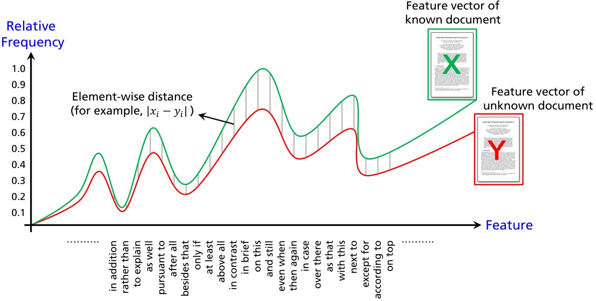
The technique requires as an input a verification case , a distance function (in the context of this paper, the Manhattan metric), a specific feature category and a corresponding threshold . The output is a triple . Here, represents a set of features, extracted from and using , associated with their element-wise distances between and . The two lists , on the other hand, divide all features into disjoint partitions. The (string-based) features contained in and are associated with adjusted distance scores that aim to “push” TAVeer towards a Y- or an N-prediction, respectively. The entire procedure for generating is described in Algorithm 1. Once and have been created, we can use them to gain insight into what specific features have contributed to the decision of TAVeer. Inspecting , for example, allows a direct comparison (cf. Figure 2) regarding the question how (dis)similar the representations of and behave to each other with respect to the features and their corresponding element-wise distances. The decisive factor here is that the investigator is not “distorted” by the prediction of the AV method, since the distances within are not dependent on any threshold. Consequently, the investigator must draw her/his own conclusions regarding the authorship of on the basis of the features and their corresponding distances contained in .
With regard to the two lists and the situation is different. These consist of tuples of the form , where represents a feature and its corresponding importance score so that the respective threshold is incorporated. Given these tuples, the investigator can see which features (and to what extent) contributed either to the Y- or an N-prediction of the AV method. To illustrate the effects of the features contained in and , we visualize (cf. Figure 3) them as vertically positioned rectangles, where green denotes Y- and red N-scores. The height of each rectangle corresponds to the importance score of a feature . Each (in the example provided in Figure 3, a topic-agnostic word that occurs at the end of a sentence) is placed to the left or right of its respective rectangle. All Y- and red N-rectangles are stacked atop each other. As a result, a given verification case is represented by two stacked bars, so that is classified as either Y or N, depending on which stacked bar is higher. Figure 3 illustrates this idea.
Here, we can see a verification case taken from the test corpus (cf. Section 6.1.3), for which the features and importance scores contained in the generated lists and are plotted as a green and red stacked bar, respectively. has been (correctly) classified as Y, since the sum of all importance scores in is bigger than the sum of the scores in .
3
5
6
7
// Assign feature and its importance score to or .
else 10
11
6 Experimental Evaluation
This section gives a detailed description of our experimental evaluation. First, we introduce our self-compiled corpora and summarize their key statistics. Next, we describe which existing baseline methods we have selected to assess the performance of TAVeer. Afterwards, we explain which performance measures we have chosen to evaluate all approaches. Finally, we present the results and describe our analytical findings.
6.1 Corpora
With regard to our experimental evaluation, we created four English corpora (cf. Table 3) covering a variety of challenges such as documents with short lengths or cross-topic conditions between unknown and known documents. In total, the corpora comprise 7,178 verification cases, which were split into author-disjunct training and test sets based on a 40/60% ratio. For each known author in the four corpora, there is exactly one Y- and one N-verification case. By this, we counteract the so-called population homogeneity bias described by Bevendorff et al. [5]. Furthermore, we ensured that all corpora are balanced so that the number of Y- and N-cases is equal. In the following, we present the four corpora in detail.
| Corpus | Genre | Topic | avg | avg | ||
| (train) | Q & A | Cross | 150 | 1 | 11,247 | 9,956 |
| (test) | posts | topics | 228 | 1 | 11,803 | 10,700 |
| (train) | Restaurant | Related | 320 | 5 | 637 | 767 |
| (test) | reviews | topics | 480 | 5 | 640 | 768 |
| (train) | Social | Mixed | 800 | 3 | 5,735 | 6,785 |
| (test) | news | topics | 1,200 | 3 | 5,854 | 6,794 |
| (train) | Product | Mixed | 1,600 | 4 | 4,010 | 4,041 |
| (test) | reviews | topics | 2,400 | 4 | 4,009 | 4,041 |
6.1.1 Stack Exchange Corpus ()
comprises 567 posts of 189 users, which have been crawled from the question-and-answer (Q & A) network Stack Exchange44 4 https://stackexchange.com in 2019. The network comprises 173 Q & A communities, where each community focuses on a specific topic. To construct , we collected both questions and answers from users that were simultaneously active on the two thematically different communities Cross Validated () and Academia (). is a strict cross-topic corpus, where each verification case comprises one known and one unknown document . With regard to the Y-cases, and stem from and , respectively, while in each N-case, and stem from the same community . Consequently, inverse predictions (i. e., N-cases are more likely to be classified as Y and vice versa) can be expected for AV methods that consider topic-related features, while topic-agnostic AV methods are more likely to withstand the cross-topic characteristic of this corpus.
6.1.2 Yelp Corpus ()
represents a collection of 2,400 comments written by 400 reviewers from the Yelp55 5 https://www.yelp.com/dataset/challenge business portal. This corpus is particularly demanding due to a number of peculiarities. First, it contains the shortest documents (compared to all other corpora), where each has a maximum length of ten sentences. Second, many reviews are written in different periods of time and often span years, which results in a distorted writing style. Third, the reviews in focus heavily on restaurants and food-related topics. Consequently, the number of relevant stylistic features is limited. Fourth, a part of the reviews contain a mixture of moderate and colloquial writing style covering a variety of slang expressions.
6.1.3 Reddit Corpus ()
consists of 4,000 posts from 1,000 users, which were crawled between 2010–2016 from the community network Reddit. In contrast to the corpora and , was designed as a mixed-topic corpus. For this, we collected for each author posts from various so-called subreddits, where each subreddit focuses on a different topic. To construct a single verification case (Y or N), we ensured that all contained documents were taken from disjoint subreddits so that all documents are thematically different from each other. In total, covers exactly 1,388 different topics including politics, science, and movies.
6.1.4 Amazon Product Data Corpus ()
is derived from the Amazon product data corpus, released by McAuley et al. [30]. The original dataset contains 142.8 million product reviews from the online-marketplace Amazon, gathered between 1996–2014. From this dataset, we extracted a subset of 10,000 reviews from 2,000 users, where each review is related to one of 17 product categories (e. g., electronics, movies and TV or office products). Similarly to the corpus, we made sure that all documents in each verification case differ from each other with respect to the product categories. Hence, also represents a mixed-topic corpus.
6.2 Existing Baselines
To measure the effectiveness of TAVeer, we have selected ten competitive AV methods as baselines, which have shown their strengths in a number of previous studies. Six of these methods (GenUnmasking [6], BAFF [5], OCCAV [15], DynamicAV [2], COAV [16] and SPATIUM [25]) were proposed in the last three years, while the remaining four methods (ProfAV [34], IM [29], NNCD [45] and Unmasking [26]) were published earlier. In the following, we describe some design decisions we have made with regard to these methods in order to apply them in our evaluation.
6.2.1 Source of Impostor Documents
IM, NNCD and SPATIUM represent extrinsic AV methods and, thus, make use of external documents to transform a verification case from a unary to a binary classification problem. In the original papers, both IM and NNCD make use of search engines to generate the impostor documents. However, due to quota limitations, we opted for an alternative strategy with regard to our reimplementations, where the impostor documents were directly taken from the test corpora. This strategy has been also considered by Kocher and Savoy [24, 25] for SPATIUM. Although using static corpora is not as flexible as using search engines, it has the advantage that due to the available metadata (for instance, user names of the authors) the true author of the unknown document is likely not among the impostors66 6 However, we cannot guarantee if different user names in fact refer to different persons. In other words, it might be possible that multiple accounts refer to the same person..
6.2.2 Uniform (Binary) Predictions
In their original form, GenUnmasking, SPATIUM and ProfAV allow the three possible prediction outputs Y (same-author), N (different-author) and U (unanswered), whereas for the remaining approaches only binary predictions (Y/N) are considered. Therefore, to enable a fair comparison, we decided to unify the predictions of all involved AV methods to the binary case. In this context, verification cases for which the AV methods determined similarity values greater than 0.5 were classified as Y, otherwise as N. Here, all similarity values were normalized into the range , so that 0.5 marks the decision threshold.
6.2.3 Settings for the Compression-Based Methods
For the compression-based AV methods NNCD, COAV and OCCAV we used the same compression algorithm PPMd as mentioned in the original papers [15, 16, 45]. However, in the respective papers it has not been mentioned how the hyperparameter model-order of PPMd has been set. We therefore decided to set this hyperparameter to 7 for all three methods, based on our observation77 7 With regard to the hyperparameter model-order, we experimented with values from 2 to 10. that this value led to the best accuracy across all our training corpora. Moreover, we used as dissimilarity functions CDM for NNCD as well as CBC for COAV and OCCAV, as defined in the original papers. Apart from these, there are no other hyperparameters for these approaches.
6.2.4 Counteracting Non-Deterministic Behavior
The four AV methods SPATIUM, IM, Unmasking and GenUnmasking involve different sources of randomness (e. g., feature subsampling, chunk generation or impostor selection) and, due to this, cause non-deterministic behavior regarding their predictions. In other words, applying these methods multiple times to the same verification case can result in different prediction outputs i. e., (Y, N, Y, …, N) which, in turn, can lead to a biased evaluation. To counteract this problem, we performed 11 runs for each non-deterministic method and selected the run (together with the calculated accuracy, AUC and the four confusion matrix outcomes) for which the accuracy score represented the median. The reason why we avoided to average the multiple runs (as, for example, was the case in [35]) was to obtain accurate numbers in regard to our analysis.
6.2.5 Model and Hyperparameters
In general, model parameters refer to parameters that are estimated directly from the data, while hyperparameters cannot be obtained directly from the data and must therefore be set manually. In regard to the AV methods considered in our experiments, model parameters represent the weights that form the SVM-hyperplanes (used by Unmasking and GenUnmasking) or scalar thresholds required to accept or reject the questioned authorships (used by COAV, ProfAV, IM and DynamicAV). To obtain the model parameters of ProfAV, IM, COAV and DynamicAV, we trained the methods on the respective training corpora.
The hyperparameters involved in our selected AV approaches represent, among others, the number of cross-validation folds (used by Unmasking and GenUnmasking) or the -order of the character -grams (used by ProfAV and DynamicAV) and have been tuned in the following way: For SPATIUM, we used the original implementations88 8 Both implementations are available at https://github.com/pan-webis-de. together with their unmodified hyperparameter settings, mentioned in the respective papers [24, 25]. Regarding ProfAV, IM, Unmasking, GenUnmasking and DynamicAV, we used our own implementations, where for the first two we employed the same hyperparameter ranges described in the original papers. For GenUnmasking, we have considered the same fixed99 9 These are: Number and size of chunks (in words): 30 chunks counting 700 words each, Initial feature set size: 250 most frequent words in each document pair, Number of cross-validation folds: 10, SVM-Kernel: linear, Number of eliminated features: 5 (positive and negative, respectively). hyperparameters mentioned in the original paper [6], whereas for Unmasking an adjustment was needed to fit our experimental setting. In the original definition of this method, Koppel and Schler [26, 28] used entire books to train and evaluate Unmasking, which differ in lengths from the documents used in our corpora. Therefore, instead of using the original fixed hyperparameter settings (which would make Unmasking inapplicable in our evaluation setting), we decided to consider individual hyperparameter ranges with values that are more appropriate for shorter documents as available in our corpora. The customized ranges are listed in Table 4.
| Hyperparameter | Our grid search range | Original setting |
| = Initial feature set sizes | 250 | |
| = Number of eliminated features | 3 | |
| = Number of iterations | 10 | |
| = Chunk sizes (in words) | 500 | |
| = Number of folds | 10 |
Based on the original and adjusted ranges, ProfAV, IM and Unmasking were optimized using the grid search algorithm, which was guided by accuracy as a performance metric. All tuned hyperparameters are listed in Table 5. For a more detailed explanation of each hyperparameter, we refer the interested reader to the original paper of the respective AV method.
| Hyperpar. | |||||
| 9,000 | 9,000 | 7,000 | 6,000 | ||
| 5,000 | 2,000 | 9,000 | 1,000 | ||
| 4 | 5 | 5 | 5 | ||
| ProfAV | |||||
| 150 | 100 | 50 | 150 | ||
| 5 | 2 | 2 | 2 | ||
| 5 | 7 | 7 | 3 | ||
| 5 | 5 | 5 | 5 | ||
| Unmasking | 10 | 7 | 7 | 7 | |
| 100 | 100 | 100 | 100 | ||
| 10 | 10 | 100 | 10 | ||
| IM | 50 | 100 | 100 | 50 | |
| Token | Lemma | Token | Token | ||
| Top % | 15 | 8 | 1 | 3 | |
| Dyn.AV | 4 | 1 | 1 | 1 |
6.2.6 Consideration of Features
With regard to the DynamicAV approach, we have discarded the feature category diacritics, based on the observation that they were very rarely present within the documents in our corpora. With regard to the POS tags used by the same method, we used the well-known spaCy1010 10 Here, we used spaCy’s integrated POS tagger (model: "en_core_web_lg") available at https://spacy.io. framework [19].
6.3 Performance Measures
To assess the performance of TAVeer, we selected accuracy as a primary measure for a number of reasons. First, accuracy has been used in numerous research works including [2, 3, 4, 10, 12, 18, 26, 31, 42] and, thus, can be seen as the most common choice in the field of AV. Second, the measure is intuitively understandable (the higher the resulting accuracy value, the lower the sum of incorrect predictions). Third, accuracy behaves symmetric in contrast to alternative performance measures (for example, F1) so that the classes Y and N are treated equally. Fourth, the measure is suitable for our purpose, since in our experiments all corpora are balanced.
For a better comparability, we also report the four confusion matrix outcomes: true positives (TP), false negatives (FN), false positives (FP) and true negatives (TN) that aim to provide a detailed insight into the predictions of the individual AV methods. Moreover, they allow the interested reader to compute other performance measures that might be useful for other comparisons. Moreover, we consider AUC as an alternative measure, which has been often used in previous AV studies including [1, 18, 35, 36, 40].
6.4 Results
After we have trained TAVeer and the ten selected baselines on the four training corpora, we evaluated all AV methods on the respective test corpora. The evaluation results are shown in Table 6. As can be seen in this table, TAVeer outperforms all ten baselines on the demanding corpus , which demonstrates its robustness under cross-topic conditions. In addition, TAVeer surpasses all baseline methods on and is ranked second on , indicating that the method is also suitable for mixed-topic corpora. On the corpus , TAVeer is on par with the strongest baseline IM, which shows that the method is also applicable in scenarios where the documents consist of a few sentences. It should be emphasized, that half of the baseline methods ( and NNCD) make use of character -grams which, according to the literature, represent the strongest features in the field of AV. In this regard, the results demonstrate that punctuation- and TA-based features alone, are similarly effective and in some cases even better.
Nevertheless, the accuracies listed in Table 6 reflect only a summary view of TAVeer’s performance. To gain an insight into what led to these results, we therefore conduct a more detailed analysis regarding our approach. For this purpose, we first take a closer look at the models TAVeer learned on the basis of the training corpora, in order to understand their behavior on the test corpora. Using the proposed interpretation technique (cf. Section 5) we then perform a more fine-grained analysis in which we investigate which specific features contributed to TAVeer’s predictions.
Method Acc. AUC TP FN FP TN TAVeer 0.697 0.778 80 34 35 79 COAV 0.404 0.388 42 72 64 50 IM 0.482 0.515 38 76 42 72 BAFF 0.531 0.545 44 70 37 77 DynamicAV 0.496 0.518 87 27 88 26 NNCD 0.513 0.552 4 110 1 113 OCCAV 0.496 0.408 0 114 1 113 ProfAV 0.539 0.609 67 47 58 56 SPATIUM 0.636 0.723 49 65 18 96 GenUnmasking 0.522 0.524 54 60 49 65 Unmasking 0.539 0.542 60 54 51 63 TAVeer 0.690 0.746 166 74 75 165 COAV 0.710 0.769 166 74 65 175 IM 0.708 0.788 150 90 50 190 BAFF 0.592 0.704 206 34 162 78 DynamicAV 0.608 0.663 178 62 126 114 NNCD 0.629 0.986 62 178 0 240 OCCAV 0.629 0.703 190 50 128 112 ProfAV 0.665 0.723 155 85 76 164 SPATIUM 0.590 0.651 93 147 50 190 GenUnmasking 0.500 0.500 0 240 0 240 Unmasking 0.596 0.639 153 87 107 133 TAVeer 0.806 0.861 455 145 88 512 COAV 0.836 0.909 503 97 100 500 IM 0.833 0.888 431 169 31 569 BAFF 0.759 0.824 422 178 111 489 DynamicAV 0.770 0.820 511 89 187 413 NNCD 0.773 0.999 328 272 0 600 OCCAV 0.778 0.851 409 191 75 525 ProfAV 0.764 0.821 453 147 136 464 SPATIUM 0.797 0.863 446 154 90 510 GenUnmasking 0.585 0.621 328 272 226 374 Unmasking 0.719 0.785 467 133 204 396 TAVeer 0.842 0.912 982 218 161 1039 COAV 0.768 0.847 925 275 281 919 IM 0.815 0.901 941 259 186 1014 BAFF 0.698 0.762 647 553 171 1029 DynamicAV 0.785 0.876 1030 170 346 854 NNCD 0.600 0.996 239 961 0 1200 OCCAV 0.738 0.810 950 250 378 822 ProfAV 0.723 0.797 861 339 326 874 SPATIUM 0.788 0.873 841 359 150 1050 GenUnmasking 0.563 0.598 662 538 511 689 Unmasking 0.725 0.801 903 297 362 838
6.4.1 Model Analysis
The models learned by TAVeer, using the procedure described in Section 4.2, contain some useful details that can help to understand the question, which feature categories are more relevant for each corpus. In the following, we take a closer look on the four generated models (cf. Table 7) to answer this question. As a starting point for our investigation, we apply TAVeer using a model to a test corpus for each Stack, Yelp, Reddit, Amazon. As a result, we obtain for each the predictions for all contained verification cases. Using Equation 4, we then compute similarity scores for all verification cases with respect to each atomic ensemble . The similarity scores for the Y- and N-cases in each , regarding the feature categories contained in each model , are visualized as violin plots in Figure 4. These plots can be interpreted as follows. The distribution of the similarity scores for each feature category are colored green and red, respectively, while the dashed line represents the decision boundary. The better this line can separate both distributions and the less they overlap, the more suitable is for the test corpus . Although no single feature category clearly separates the distributions across all corpora, we can still observe a number of tendencies. Regarding and , for example, it can be seen in Figure 4 that (punctuation -grams) are among the strongest feature categories. The degree of overlap between the distributions of is smaller in comparison to the other feature categories, while at the same time, the decision boundary can better separate them. When focusing on (TA sentence and clause starters), it can further be seen that this feature category is also important for these three corpora, while for it plays only a minor role. With regard to , is primarily relevant, while the remaining feature categories contribute similarly to the overall prediction. Moreover, for the mixed-topic corpora and , it can be seen that (TA token -Grams) also represents a strong feature category, based on the observation that the distributions (in both and ) only intersect in a small region around the decision boundary.
Corpus
6.4.2 Feature Analysis
So far, we investigated the question which particular feature categories were more relevant regarding the four test corpora. In the following, we take a closer look at the classification results of TAVeer with respect to six verification cases originating from the test corpus . Here, the cases and were correctly classified as Y (true positives) and N (true negatives), respectively. To perform the analysis, we use our interpretation method introduced in Section 5. Recall that this method consumes as input a verification case , an atomic ensemble , and a distance function dist. The output are two disjunct lists and comprising tuples of the form , where represents a feature and its corresponding importance score. Given these tuples, we can see which features (and to what extent) contributed either to the Y- or N-prediction of TAVeer. In our model analysis we found that was one of the strongest feature categories across all test corpora. Therefore, we focus on this feature category in the following. After applying Algorithm 1 to the six verification cases, we obtain for each a pair of two lists and . The impact of these features are visualized in Figure 5.
From the illustration in Figure 5 a number of observations can be made. Regarding , for example, it can be seen that -features are missing, which explains why achieved the highest similarity value of all verification cases. While inspecting the occurrences of the -features ;(’):- in the documents within , we noticed that their frequency distributions were almost equal.
For , it can be noticed that almost each -feature is more important than the single -feature. In other words, the hyphen - is the only feature that led to a (small) discrepancy between the frequency distributions of all punctuation marks in and within . For , we can see that the six punctuation marks ();-.: are sufficient for its correct Y-prediction. In contrast, only the two punctuation marks .’ are required to correctly classify as N. With regard to it is further shown that the -feature ’ is the most important feature, which alone is sufficient to distinguish the authorships in all three cases. The importance score of this feature points to a greater usage of contractions, which are only (or mostly) present in one document. Overall, we can conclude from these observations that correct predictions can be achieved with just a few features.
7 Conclusion and Future Work
We discussed an important problem in the field of authorship verification, which occurs when an AV method has no control over the features it captures. In the worst case, the prediction of the method may be based on topic-related words rather than on stylistic features, so that the AV method will miss its true purpose. To address this problem, we have made three contributions. First, we proposed a number of feature categories that comprise a wide spectrum of topic-agnostic (TA) features. Second, we proposed an effective distance-based AV method called TAVeer, which considers solely these feature categories for its classification predictions. Third, we proposed an interpretation scheme that allows to understand which features contributed to TAVeer’s prediction.
To assess our approach, we performed a comprehensive evaluation with ten existing AV approaches applied to four corpora with related-, cross- and mixed topics. In this regard, we have demonstrated that our method outperforms all baseline methods with respect to one cross-topic and one mixed-topic corpus, while on the other two corpora, TAVeer performs close to the strongest baseline COAV. In a detailed analysis with respect to the models learned by TAVeer, we have shown that punctuation -grams (for ), TA sentence and clause starters and TA token unigrams were the strongest feature categories across all four test corpora. Furthermore, we have shown in a fine-grained feature analysis that a small number of features is sufficient to correctly classify challenging cross-topic verification cases (two and six features for a N- and Y-case, respectively).
Nevertheless, our AV method leaves room for further improvements. Currently, TAVeer does not take into account misspelled words, which can lead to a loss of potentially relevant features, especially in connection with informal texts. We therefore leave for future work the investigation of effective possibilities to semantically match misspelled words with respect to their common entity. One idea, for example, is to use back-translation services that can handle difficult spelling mistakes, which cannot be corrected by standard spell checkers. Furthermore, we plan to find a better alternative to visualize the features derived from the interpretation scheme more clearly (ideally in the document itself). However, this requires a careful consideration how to map the importance scores of the features (across all feature categories) to respective colors without to cause overplotting. A further direction for future work is to investigate alternative feature categories not yet been considered in this paper. In this context, one idea is to experiment with interjections (e. g., "lol" or "aha") or topic-agnostic abbreviations (for example, "e.g." or "etc."), which represent important idiosyncratic stylistic markers. Another question we want to address in future work is how TAVeer behaves under cross-domain conditions. These are of particular relevance as they often occur in real forensic cases (e. g., how a model trained on forum posts or cooking recipes performs on suicide letters, for which no training data is available).
8 Acknowledgments
This research work has been funded by the German Federal Ministry of Education and Research and the Hessen State Ministry for Higher Education, Research and the Arts within their joint support of the National Research Center for Applied Cybersecurity ATHENE. We would like to thank Christian Winter and Inna Vogel for their valuable reviews that helped to improve the quality of this paper.
References
- [1] Sasa Adamovic, Vladislav Miskovic, Milan Milosavljevic, Marko Sarac, and Mladen Veinovic. Automated Language-independent Authorship Verification (for Indo-European Languages). Journal of the Association for Information Science and Technology, 70(8):858–871, 2019.
- [2] Hossam Ahmed. The Role of Linguistic Feature Categories in Authorship Verification. Procedia Computer Science, 142:214 – 221, 2018. Arabic Computational Linguistics.
- [3] Sylvio Barbon, Jr, Rodrigo Augusto Igawa, and Bruno Bogaz Zarpelão. Authorship Verification Applied to Detection of Compromised Accounts on Online Social Networks. Multimedia Tools Appl., 76(3):3213–3233, February 2017.
- [4] N. E. Benzebouchi, N. Azizi, M. Aldwairi, and N. Farah. Multi-Classifier System for Authorship Verification Task Using Word Embeddings. In 2018 2nd International Conference on Natural Language and Speech Processing (ICNLSP), pages 1–6, April 2018.
- [5] Janek Bevendorff, Matthias Hagen, Benno Stein, and Martin Potthast. Bias Analysis and Mitigation in the Evaluation of Authorship Verification. In Anna Korhonen, David R. Traum, and Lluís Màrquez, editors, Proceedings of the 57th Conference of the Association for Computational Linguistics, ACL 2019, Florence, Italy, July 28- August 2, 2019, Volume 1: Long Papers, pages 6301–6306. Association for Computational Linguistics, 2019.
- [6] Janek Bevendorff, Benno Stein, Matthias Hagen, and Martin Potthast. Generalizing Unmasking for Short Texts. In Proceedings of the 2019 Conference of the North American Chapter of the Association for Computational Linguistics: Human Language Technologies, Volume 1 (Long and Short Papers), pages 654–659, Minneapolis, Minnesota, June 2019. Association for Computational Linguistics.
- [7] José Nilo G. Binongo. Who Wrote the 15th Book of Oz? An Application of Multivariate Analysis to Authorship Attribution. CHANCE, 16(2):9–17, 2003.
- [8] M. L. Brocardo, I. Traore, S. Saad, and I. Woungang. Authorship Verification for Short Messages Using Stylometry. In 2013 International Conference on Computer, Information and Telecommunication Systems (CITS), pages 1–6, May 2013.
- [9] John Burrows. ’Delta’: a Measure of Stylistic Difference and a Guide to Likely Authorship. Literary and Linguistic Computing, 17(3):267–287, 2002.
- [10] Daniel Castro Castro, Yaritza Adame Arcia, María Pelaez Brioso, and Rafael Muñoz Guillena. Authorship Verification, Average Similarity Analysis. In Proceedings of the International Conference Recent Advances in Natural Language Processing, pages 84–90. INCOMA Ltd. Shoumen, BULGARIA, 2015.
- [11] R. Chandrasekaran and G. Manimannan. Use of Generalized Regression Neural Network in Authorship Attribution. International Journal of Computer Applications, 62(4):7–10, January 2013.
- [12] Xiaoling Chen, Peng Hao, R. Chandramouli, and K. P. Subbalakshmi. Authorship Similarity Detection from Email Messages. In Proceedings of the 7th International Conference on Machine Learning and Data Mining in Pattern Recognition, MLDM’11, pages 375–386, Berlin, Heidelberg, 2011. Springer-Verlag.
- [13] Tom De Smedt and Walter Daelemans. Pattern for Python. J. Mach. Learn. Res., 13(1):2063–2067, June 2012.
- [14] Michael Gamon. Linguistic Correlates of Style: Authorship Classification with Deep Linguistic Analysis Features. In Proceedings of Coling 2004, pages 611–617. International Conference on Computational Linguistics, August 2004.
- [15] Oren Halvani, Lukas Graner, and Inna Vogel. Authorship Verification in the Absence of Explicit Features and Thresholds. In Gabriella Pasi, Benjamin Piwowarski, Leif Azzopardi, and Allan Hanbury, editors, Advances in Information Retrieval, pages 454–465. Springer International Publishing, 2018.
- [16] Oren Halvani, Christian Winter, and Lukas Graner. On the Usefulness of Compression Models for Authorship Verification. In Proceedings of the 12th International Conference on Availability, Reliability and Security, ARES ’17, pages 54:1–54:10, New York, NY, USA, 2017. ACM.
- [17] Oren Halvani, Christian Winter, and Lukas Graner. Assessing the Applicability of Authorship Verification Methods. In Proceedings of the 14th International Conference on Availability, Reliability and Security, ARES 2019, Canterbury, UK, August 26-29, 2019, pages 38:1–38:10. ACM, 2019.
- [18] Ángel Hernández-Castañeda and Hiram Calvo. Author Verification Using a Semantic Space Model. Computación y Sistemas, 21(2), 2017.
- [19] Matthew Honnibal and Mark Johnson. An Improved Non-monotonic Transition System for Dependency Parsing. In Proceedings of the 2015 Conference on Empirical Methods in Natural Language Processing, pages 1373–1378, Lisbon, Portugal, September 2015. Association for Computational Linguistics.
- [20] Magdalena Jankowska, Evangelos E. Milios, and Vlado Keselj. Author Verification Using Common N-Gram Profiles of Text Documents. In Jan Hajic and Junichi Tsujii, editors, COLING 2014, 25th International Conference on Computational Linguistics, Proceedings of the Conference: Technical Papers, August 23-29, 2014, Dublin, Ireland, pages 387–397. ACL, 2014.
- [21] Patrick Juola, John Noecker, Ariel Stolerman, Michael Ryan, Patrick Brennan, and Rachel Greenstadt. Towards Active Linguistic Authentication. In Gilbert Peterson and Sujeet Shenoi, editors, Advances in Digital Forensics IX, pages 385–398, Berlin, Heidelberg, 2013. Springer Berlin Heidelberg.
- [22] Patrick Juola and Efstathios Stamatatos. Overview of the Author Identification Task at PAN 2013. In Working Notes for CLEF 2013 Conference, Valencia, Spain, September 23-26, 2013, 2013.
- [23] Mahmoud Khonji and Youssef Iraqi. A Slightly-Modified GI-Based Author-Verifier with Lots of Features (ASGALF). In Working Notes for CLEF 2014 Conference, Sheffield, UK, September 15-18, 2014., pages 977–983, 2014.
- [24] Mirco Kocher and Jacques Savoy. Unine at CLEF 2015 author identification: Notebook for PAN at CLEF 2015. In CLEF (Working Notes), volume 1391 of CEUR Workshop Proceedings. CEUR-WS.org, 2015.
- [25] Mirco Kocher and Jacques Savoy. A Simple and Efficient Algorithm for Authorship Verification. Journal of the Association for Information Science and Technology, 68(1):259–269, 2017.
- [26] Moshe Koppel and Jonathan Schler. Authorship Verification as a One-Class Classification Problem. In Carla E. Brodley, editor, Machine Learning, Proceedings of the Twenty-first International Conference (ICML 2004), Banff, Alberta, Canada, July 4-8, 2004, volume 69 of ACM International Conference Proceeding Series. ACM, 2004.
- [27] Moshe Koppel, Jonathan Schler, and Shlomo Argamon. Computational Methods in Authorship Attribution. JASIST, 60(1):9–26, 2009.
- [28] Moshe Koppel, Jonathan Schler, and Elisheva Bonchek-Dokow. Measuring Differentiability: Unmasking Pseudonymous Authors. J. Mach. Learn. Res., 8:1261–1276, December 2007.
- [29] Moshe Koppel and Yaron Winter. Determining if Two Documents are Written by the Same Author. JASIST, 65(1):178–187, 2014.
- [30] Julian McAuley, Christopher Targett, Qinfeng Shi, and Anton van den Hengel. Image-Based Recommendations on Styles and Substitutes. In Proceedings of the 38th International ACM SIGIR Conference on Research and Development in Information Retrieval, SIGIR ’15, pages 43–52, New York, NY, USA, 2015. ACM.
- [31] Jan Christoph Meister, editor. Evaluating Unmasking for Cross-Genre Authorship Verification, Hamburg, Germany, 2012.
- [32] Tempestt J. Neal, Kalaivani Sundararajan, and Damon L. Woodard. Exploiting Linguistic Style as a Cognitive Biometric for Continuous Verification. In 2018 International Conference on Biometrics, ICB 2018, Gold Coast, Australia, February 20-23, 2018, pages 270–276. IEEE, 2018.
- [33] Daniel Pavelec, Luiz S. Oliveira, Edson J. R. Justino, and Leonardo Vidal Batista. Using conjunctions and adverbs for author verification. J. UCS, 14(18):2967–2981, 2008.
- [34] Nektaria Potha and Efstathios Stamatatos. A Profile-Based Method for Authorship Verification. In Artificial Intelligence: Methods and Applications: 8th Hellenic Conference on AI, SETN 2014, Ioannina, Greece, May 15–17, 2014. Proceedings, pages 313–326. Springer International Publishing, 2014.
- [35] Nektaria Potha and Efstathios Stamatatos. An Improved Impostors Method for Authorship Verification. In Experimental IR Meets Multilinguality, Multimodality, and Interaction - 8th International Conference of the CLEF Association, CLEF 2017, Dublin, Ireland, September 11-14, 2017, Proceedings, pages 138–144, 2017.
- [36] Nektaria Potha and Efstathios Stamatatos. Dynamic Ensemble Selection for Author Verification. In Leif Azzopardi, Benno Stein, Norbert Fuhr, Philipp Mayr, Claudia Hauff, and Djoerd Hiemstra, editors, Advances in Information Retrieval, pages 102–115, Cham, 2019. Springer International Publishing.
- [37] Nektaria Potha and Efstathios Stamatatos. Improved Algorithms for Extrinsic Author Verification. Knowledge and Information Systems, Oct 2019.
- [38] O. Srinivasa Rao, N. V. Ganapathi Raju, and V. Vijaya Kumar. Authorship attribution on imbalanced english editorial corpora. International Journal of Computer Applications, 169(1):44–47, Jul 2017.
- [39] Shachar Seidman. Authorship Verification Using the Impostors Method Notebook for PAN at CLEF 2013. In Working Notes for CLEF 2013 Conference , Valencia, Spain, September 23-26, 2013., 2013.
- [40] Efstathios Stamatatos, Walter Daelemans, Ben Verhoeven, Patrick Juola, Aurelio López-López, Martin Potthast, and Benno Stein. Overview of the Author Identification Task at PAN 2015. In Working Notes of CLEF 2015 – Conference and Labs of the Evaluation forum, Toulouse, France, September 8–11, 2015, 2015.
- [41] Efstathios Stamatatos, Walter Daelemans, Ben Verhoeven, Benno Stein, Martin Potthast, Patrick Juola, Miguel A. Sánchez-Pérez, and Alberto Barrón-Cedeño. Overview of the Author Identification Task at PAN 2014. In Working Notes for CLEF 2014 Conference, Sheffield, UK, September 15–18, 2014, pages 877–897, 2014.
- [42] Magnus Stavngaard, August Sørensen, Stephan Lorenzen, Niklas Hjuler, and Stephen Alstrup. Detecting Ghostwriters in High Schools. CoRR, abs/1906.01635, 2019.
- [43] Ariel Stolerman. Authorship Verification. PhD thesis, 2015. UMI Dissertations Publishing 2015.
- [44] Paulo Varela, Edson Justino, and Luiz Soares de Oliveira. Verbs and Pronouns for Authorship Attribution. 01 2010.
- [45] Cor J. Veenman and Zhenshi Li. Authorship Verification with Compression Features. In Working Notes for CLEF 2013 Conference , Valencia, Spain, September 23–26, 2013, 2013.
- [46] Ying Zhao and Justin Zobel. Effective and Scalable Authorship Attribution Using Function Words. In GaryGeunbae Lee, Akio Yamada, Helen Meng, and SungHyon Myaeng, editors, Information Retrieval Technology, volume 3689 of Lecture Notes in Computer Science, pages 174–189. Springer Berlin Heidelberg, 2005.
- [47] Ying Zhao, Justin Zobel, and Phil Vines. Using relative entropy for authorship attribution. In Hwee Tou Ng, Mun-Kew Leong, Min-Yen Kan, and Donghong Ji, editors, Information Retrieval Technology, pages 92–105, Berlin, Heidelberg, 2006. Springer Berlin Heidelberg.