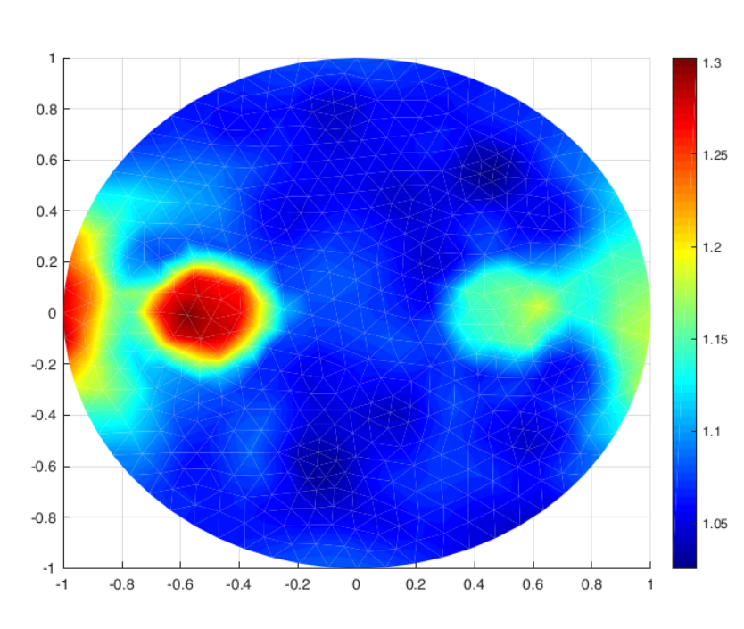
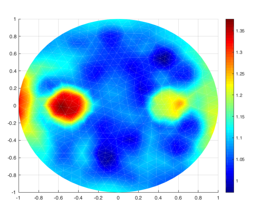
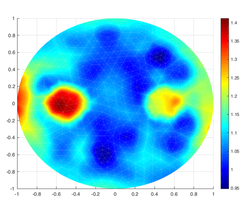
跳到论文正文
W Papers独立论文阅读器 arXiv:2006.12299 论文正文 计算阅读时间 · 0%
引用这篇论文根据当前论文元数据生成,正式投稿前建议核对。


License: arXiv.org perpetual non-exclusive license
arXiv:2006.12299v2 [math.AP] 17 Dec 2020

Uniqueness, Lipschitz stability and reconstruction for the inverse optical tomography problem Thanks: Submitted to the editors DATE.

Houcine Meftahi Email: houcine.meftahi@enit.utm.tn Thanks: Department of Mathematics, ENIT of Tunisia .
Abstract

In this paper, we consider the inverse problem of recovering a diffusion σ\sigma and absorption coefficients qq in steady-state optical tomography problem from the Neumann-to-Dirichlet map. We first prove a Global uniqueness and Lipschitz stability estimate for the absorption parameter provided that the diffusion σ\sigma is known and show how to quantify the Lipschitz stability constant for a given setting. Then, we prove a Lipschitz stability result for simultaneous recovery of σ\sigma and qq. In both cases the parameters belong to a known finite subspace with a priori known bounds. The proofs rely on a monotonicity result combined with the techniques of localized potentials. To numerically solve the inverse problem, we propose a Kohn-Vogelius-type cost functional over a class of admissible parameters subject to two boundary value problems. The reformulation of the minimization problem via the Neumann-to-Dirichlet operator allows us to obtain the optimality conditions by using the Fréchet differentiability of this operator and its inverse. The reconstruction is then performed by means of an iterative algorithm based on a quasi-Newton method. Finally, we illustrate some numerical results.

keywords
Optical tomography, Inverse problem, Uniqueness, Lipschitz stability, Monotonicity, Localized potentials.
††runningheads: Uniqueness Lipschitz stability and reconstruction / H. Meftahi
AMS
78A46, 65J22, 65M32, 35R30

1 Introduction

In this paper, we consider the inverse problem of recovering the parameters σ⁡(x)\sigma(x) and q⁡(x)q(x) in the elliptic partial differential equation

−∇⋅(σ∇u)+qu=0 in Ω,-\nabla\cdot(\sigma\nabla u)+qu=0\textrm{ in }\Omega, (1)

from the knowledge of all possible Cauchy data on the boundary ∂Ω\partial\Omega, σ​∂νu|∂Ω,u|∂Ω\sigma\partial_{\nu}u|_{\partial\Omega},u|_{\partial\Omega}.
Problem (1) can be viewed as steady-state diffusion optical tomography, where light propagation is modeled by a diffusion approximation and the excitation frequency is set to zero. Here uu represents the density of photons, σ\sigma the diffuse coefficient and qq the optical absorption. This problem arises in medical imaging and in geophysics, for example, in reflection seismology assuming a description in terms of time-harmonic scalar waves. For a full description of optical tomography, we refer the reader to the topical reviews of Arridge [1] and Gibson, Hebden and Arridge [2].

Although it is common practice in optical tomography to use the Robin-to-Robin map to describe the boundary measurements (see [1, 3]), the Neumann-to-Dirichlet map will be employed here instead. This is justified by the fact that in optical tomography, prescribing the Neumnann to-Dirichlet map, is equivalent to prescribing the Robin-to-Robin boundary map as long as there are no additional unknown coefficients in the Robin conditions (see for instance [4]).
The paper is split into three parts. Part one is on proving uniqueness and Lipschitz stability of the the absorption coefficient qq provided that the diffusion coefficient σ\sigma is known. Part two is on proving Lipschitz stability of σ\sigma and qq simultaneously. Part three deals with the reconstruction of σ\sigma and qq based on minimizing a Kohn-Vogelius type functional.

The inverse problem of recovering qq from the knowledge of the Dirichlet-to-Neumann map was first introduced (in a slightly different setting) by Calderón in [5]. The uniqueness issue was treated by Sylvester and Uhlmann in [6]. For more recent result on uniqueness, we refer the reader to [7]. By virtue of the work of Alessandrini [8] it is known that both problems of recovering σ\sigma or qq (in suitable regularity scales) enjoy logarithmic stability estimates under mild a priori assumptions on the data. As shown by Mandache [9], this log-type estimate is optimal. Thus for arbitrary potentials qq, Lipschitz stability cannot hold. As discovered in [10], considering potentials or conductivities in certain finite-dimensional spaces provides improvements in terms of stability. Under certain assumptions, the authors prove Lipschitz stability estimates. Their argument relies on a combination of singular solutions and unique continuation estimates. This idea has been extended to more complex equations and systems (see for instance [11, 12, 13, 14, 15, 16]).

As a key novelty in this article, we present a different approach based on the monotonicity and the techniques of localized potentials instead of combining singular solutions with unique continuation results as previously done in the literature. Following analogous results in electrical impedance tomography and elasticity [17, 18, 19], here we will study the question whether the coefficient qq can be uniquely and stably reconstructed. More precisely, we show that qq is uniquely determined and depends upon the Neumaun-to-Dircihlet map of (1) in a Lipschitz way as long as supp⁡(q)⋐Ω\rm{supp}(\it q)\Subset\Omega and σ\sigma is known. Moreover, we quantify the Lipschitz constant for a given setting by solving a finite number of well-posed PDEs which may be important to quantify the noise robustness in practical applications. To our best knowledge, this result of quantitative Lipschitz stability is new for the problem under consideration.

As mentioned in [20], the inverse problem of simultaneous reconstruction of σ\sigma and qq is in general not uniquely solvable, i.e., it is not possible to uniquely determine both σ\sigma and qq from boundary data of uu provided that σ\sigma and qq are smooth. The reason is that a diffusion coefficient can be transformed into an absorption coefficient by setting

v:=σ​u,v:=\sqrt{\sigma}u,

which transforms equation (1) into

−Δ​v+c​v=0,c=Δ​σσ+qσ.-\Delta v+cv=0,\quad c=\frac{\Delta\sqrt{\sigma}}{\sqrt{\sigma}}+\frac{q}{\sigma}.

If σ=1\sigma=1 in a neighborhood of ∂Ω\partial\Omega, then the boundary values remain unchanged. Hence, boundary measurements can only contain information about cc, from which one cannot extract σ\sigma and qq. Despite this negative theoretical result, a prominent result by Harrach [4] demonstrates that uniqueness holds for piecewise constant diffusion and piecewise analytic absorption coefficients. The author proves that under this condition both parameters are simultaneously uniquely determined by knowledge of all possible pairs of Neumann and Dirichlet boundary values σ∂ν|S,u|S\sigma\partial_{\nu}|_{S},u|_{S}, of solutions uu of (1), and SS is a non-empty subset of ∂Ω\partial\Omega

In this paper, we go a step further and we prove a Lipschitz stability for the inverse problem of recovering qq and σ\sigma simultaneously. The proof relies on a monotonicity estimates combined with the techniques of localized potentials. To the author’s knowledge the Lipschitz stability presented in this work is the first result on simultaneous recovery for a class of real-valued diffusion and absorption coefficients.

The idea of using monotonicity and localized potentials method has lead to a several results for inverse coefficient problems; see for instance [21, 22, 23, 24, 25, 26, 27, 28]. Together with the recent results [29, 18, 17, 19], this work shows that this idea can also be used to prove Uniqueness and Lipschitz stability results for the inverse optical tomography problem.

Lipschitz stability estimates for inverse and ill-posed problems are usually based on constructive approaches involving Carleman estimates or quantitative estimates of unique continuation [30, 14, 31, 32, 33, 34, 35]. For some applications these constructive approaches also allowed to quantify the asymptotic behavior of the Lipschitz constant; see for instance [36].

Our approach on proving Lipschitz stability is relatively simple compared to previous works. The main tools are: standard (non quantitative) unique continuation, the monotonicity result and the method of localized potentials.

For the numerical solution, we reformulate the inverse problem into a minimization problem using a Kohn-Vogelius functional, and use a quasi-Newton method which employs the analytic gradient of the cost function and the approximation of the inverse Hessian is updated by BFGS scheme [37]. Let us stress that this numerical part approaches the problem from a heuristic numerical side to demonstrate that useful numerical reconstructions are indeed possible. It remains a challenging open task how to unite the theoretical and numerical approaches in order to find rigorously justified reconstruction methods that work well in practically relevant settings.

Let us recall that in [38, 39, 40, 41], the authors propose new algorithms for recovering optical material properties. These algorithmes are experimentally tested for two and three- dimensional cases. While these works, which address real-life three-dimensional problems are an important step towards practical applications, they still suffer from considerable cross-talk between absorption and scattering reconstructions. What we mean by cross-talk is that purely scattering (or purely absorbing) inclusions are often reconstructed with unphysical absorption (or scattering) properties. This behavior is well-understood from the theoretical viewpoint: Different optical distributions inside the medium can lead to the same measurements collected at the surface of the medium [20, 42]. To avoid such cross-talks for our numerical results, we have used a suitable regularization techniques for the proposed algorithm in order to better separate and estimate simultaneously the optical properties σ\sigma and qq.

The paper is organized as follows. In section 2, we introduce the forward, the Neumann-to-Dirichlet operator and the inverse problem. Section 3 and 4 contain the main theoretical tools for this work. Section 3 is devoted to the reconstruction of the absorption coefficient assuming that the diffusion coefficient is known. We show a monotonicity relation and we prove a Runge approximation result. Then we deduce the existence of localized potentials and prove the global uniqueness and Lipschitz stability estimate and show how to calculate the Lipschitz stability constant for a given setting. Section 4 is concerned with the reconstruction of the diffusion and the absorption coefficients simultaneously. We first show a monotonicity result between the diffusion and absorption coefficients and the Neumann-to-Dirichlet operator and prove the existence of localized potentials. Then, we prove the Lipschitz stability estimate. In section 5, we introduce the minimization problem, and we compute the first order optimality condition. In section 6, satisfactory numerical results for two-dimensional problem are presented. The last section contains some concluding remarks.

2 Problem formulation

Let Ω⊂ℝd\Omega\subset\mathbb{R}^{d} (d≥2d\geq 2), be a bounded domain with smooth boundary ∂Ω\partial\Omega. For σ,q∈L+∞​(Ω)\sigma,q\in L^{\infty}_{+}(\Omega), where L+∞L^{\infty}_{+} denotes the subset of L∞L^{\infty}-functions with positive essential infima, we consider the following problem with Neumann boundary data g∈L2​(∂Ω)g\in L^{2}(\partial\Omega):

{−∇⋅(σ∇u)+qu=0 in Ω,σ∂νu=g on ∂Ω,\left\{\eqalign{-\nabla\cdot(\sigma\nabla u)+qu=0\quad\textrm{ in }\Omega,\\ \sigma\partial_{\nu}u=g\quad\textrm{ on }\partial\Omega,}\right. (2)

where ν\nu is the unit normal vector to ∂Ω\partial\Omega. The weak formulation of problem (2) reads

∫Ωσ∇u⋅∇wdx+∫Ωquwdx=∫∂Ωgwds for all w∈H1(Ω).\int_{\Omega}\sigma\nabla u\cdot\nabla w\,dx+\int_{\Omega}quw\,dx=\int_{\partial\Omega}gw\,ds\textrm{ for all }w\in H^{1}(\Omega). (3)

Using the Riesz representation theorem (or the Lax-Milgram-Theorem), it is easily seen that (3) is uniquely solvable and that the solution depends continuously on g∈L2​(∂Ω)g\in L^{2}(\partial\Omega) and σ,q∈L+∞​(Ω)\sigma,q\in L^{\infty}_{+}(\Omega). Then, we can define the Neumann-to-Dirichlet operator (NtD):

Λ⁡(σ,q):L2​(∂Ω)⟶L2​(∂Ω)g⟼u|∂Ω,\eqalign{\Lambda(\sigma,q):L^{2}(\partial\Omega)&\longrightarrow L^{2}(\partial\Omega)\cr&g\longmapsto u_{|\partial\Omega},}

The inverse problem we consider here, is the following:

 Find the parameters ​σ,q​ from the knowledge of the map ​Λ​(σ,q).\textrm{ \it Find the parameters }\sigma,q\textrm{ \it from the knowledge of the map }\Lambda(\sigma,q). (4)

We will consider diffusion and absorption parameters that are a priori known to belong to a finite dimensional set of piecewise-analytic functions and that are bounded from above and below by a priori known constants. To that end, we first define piecewise-analyticity as in [17, Definition 2.1]

Definition 1.
  • (a)

    A Subset Γ⊆∂Ω\Gamma\subseteq\partial\Omega of the boundary of an open set Ω⊂ℝn\Omega\subset\mathbb{R}^{n} is called a smooth boundary piece if it is a C∞C^{\infty}-surface and Ω\Omega lies on one side of it, i.e. if for each z∈Γz\in\Gamma there exists a ball Bϵ​(z)B_{\epsilon}(z) and function γ∈C∞​(ℝn−1,ℝ)\gamma\in C^{\infty}(\mathbb{R}^{n-1},\mathbb{R}) such that

    Γ=∂Ω∩Bϵ​(z)={x∈Bϵ​(z):xn=γ⁡(x1,…,xn−1)},\Gamma=\partial\Omega\cap B_{\epsilon}(z)=\left\{x\in B_{\epsilon}(z):x_{n}=\gamma(x_{1},\ldots,x_{n-1})\right\},
    Ω∩Bϵ​(z)={x∈Bϵ​(z):xn>γ⁡(x1,…,xn−1)}.\Omega\cap B_{\epsilon}(z)=\left\{x\in B_{\epsilon}(z):x_{n}>\gamma(x_{1},\ldots,x_{n-1})\right\}.
  • (b)

    Ω\Omega is said to have smooth boundary if ∂Ω\partial\Omega is a union of smooth boundary pieces. Ω\Omega is said to have piecewise smooth boundary if ∂Ω\partial\Omega is a countable union of the closures of smooth boundary pieces.

  • (c)

    A function φ∈L∞​(Ω)\varphi\in L^{\infty}(\Omega) is called piecewise constant if there exists finitely many pairwise disjoint subdomains Ω1,…,ΩN⊂Ω\Omega_{1},\ldots,\Omega_{N}\subset\Omega with piecewise smooth boundaries, such that Ω¯=Ω1∪,…,∪ΩN¯\overline{\Omega}=\overline{\Omega_{1}\cup,\ldots,\cup\Omega_{N}} and φ|Ωi\varphi|_{\Omega_{i}} is constant, i=1,…,Ni=1,\ldots,N.

  • (d)

    A function φ∈L∞​(Ω)\varphi\in L^{\infty}(\Omega) is called piecewise analytic if there exists finitely many pairwise disjoint subdomains Ω1,…,ΩN⊂Ω\Omega_{1},\ldots,\Omega_{N}\subset\Omega with piecewise smooth boundaries, such that Ω¯=Ω1∪,…,∪ΩN¯\overline{\Omega}=\overline{\Omega_{1}\cup,\ldots,\cup\Omega_{N}}, and φ|Ωi\varphi|_{\Omega_{i}} has an extension which is (real-)analytic in a neighborhood of Ωi¯\overline{\Omega_{i}}, i=1,…,Ni=1,\ldots,N.

As mentioned in [17], it is not clear whether the sum of two piecewise-analytic functions is always piecewise-analytic, i.e. whether the set of piecewise-analytic functions is a vector space. However, this can be guaranteed with a slightly stronger definition of piecewise analyticity (see [43, lemma 1]). Therefore, we make the following definition.

Definition 2.

A set ℱ⊆L∞​(Ω)\mathcal{F}\subseteq L^{\infty}(\Omega) is called a finite-dimensional subset of
piecewise-analytic functions if its linear span

spanℱ={∑j=1kλjfj:k∈ℕ,λj∈ℝ,fj∈ℱ}⊆L∞(Ω,\textrm{span}\;\mathcal{F}=\left\{\sum_{j=1}^{k}\lambda_{j}f_{j}:k\in\mathbb{N},\lambda_{j}\in\mathbb{R},f_{j}\in\mathcal{F}\right\}\subseteq L^{\infty}(\Omega,

contains only piecewise-analytic functions and dim(span 𝑂𝑃𝐸𝑁ℱ)<∞\mathcal{F})<\infty.

3 Recovery of the absorption coefficient

In this section, we assume that σ=σ0​χΩ∖ω+σ1​χω\sigma=\sigma_{0}\chi_{\Omega\setminus\omega}+\sigma_{1}\chi_{\omega}, and q=q​χωq=q\chi_{\omega}, where σ0,σ1\sigma_{0},\sigma_{1} are positive constants and ω⋐Ω\omega\Subset\Omega. We aim to recover the absorption parameter q∈L+∞​(ω)q\in L^{\infty}_{+}(\omega) from the NtD operator

Λ⁡(q):L2​(∂Ω)→L2​(∂Ω):g↦u|∂Ω.\Lambda(q):L^{2}(\partial\Omega)\to L^{2}(\partial\Omega):g\mapsto u|_{\partial\Omega}.

provided that σ\sigma is known.

Given a finite-dimensional subset ℱ\mathcal{F} of piecewise analytic functions and two constants b>a>0b>a>0, we denote the set

ℱ[a,b]:={q∈ℱ:a≤q(x)≤b, for all x∈ω}.\mathcal{F}_{[a,b]}:=\left\{q\in\mathcal{F}:\quad a\leq q(x)\leq b,\quad\textrm{ for all }x\in\omega\right\}.

Throughout this paper, the domain ω\omega, the finite-dimensional subset ℱ\mathcal{F} and the bounds b>a>0b>a>0 are fixed, and the constants in the Lipschitz stability results will depend on them. Our first results show Uniqueness and Lipschitz stability for the inverse absorption problem in ℱ[a,b]\mathcal{F}_{[a,b]}, when the complete infinite-dimensional NtD-operator is measured.
The outline of this section is the following

  • (i)(i)

    In Subsection 3.1, we prove a runge approximation result and we deduce a global uniqueness for determining qq from Λ⁡(q)\Lambda(q).

  • (i​i)(ii)

    In Subsection 3.2, we show a monotonicity and localized potentials results and we deduce a Lipschitz stability estimate for determining qq from Λ⁡(q)\Lambda(q).

  • (i​i​i)(iii)

    In Subsection 3.3, we show how to quantify the Lipschitz constant.

3.1 Runge approximation and uniqueness.

We first note the following unique continuation property. For every open connected subset 𝒪⊂Ω\mathcal{O}\subset\Omega, only the trivial solution of

−div(σ∇u)+qu=0 in 𝒪,-{\rm div}(\sigma\nabla u)+qu=0\textrm{ in }\mathcal{O},

vanishes on an open subset of 𝒪\mathcal{O} or possesses zero Cauchy data on a smooth, open part of ∂𝒪\partial\mathcal{O}. When σ\sigma is Lipschitz and qq is bounded, this property is proven in Miranda [44, Thm. 19, II]. It can be extended to the case of piecewise analytic σ\sigma and qq by sequentially solving Cauchy problems (see [45]).

We will deduce the uniqueness theorem 4 from the following Runge approximation result.

Theorem 3 (Runge approximation).

Let q∈L+∞​(ω)q\in L^{\infty}_{+}(\omega) be piecewise analytic. For all f∈L2​(ω)f\in L^{2}(\omega) there exists a sequence (gn)n∈ℕ⊂L2​(∂Ω)(g_{n})_{n\in\mathbb{N}}\subset L^{2}(\partial\Omega) such that the corresponding solutions u(gn)u^{(g_{n})} of (2) with boundary data gng_{n}, n∈ℕn\in\mathbb{N}, fulfill

u(gn)|ω→f in ​L2​(ω).u^{(g_{n})}|_{\omega}\to f\quad\textrm{ in }L^{2}(\omega).

Proof.

We introduce the operator

A:L2(ω)→L2(∂Ω),f↦Af:=v|∂Ω,A:L^{2}(\omega)\to L^{2}(\partial\Omega),\quad f\mapsto Af:=v_{|\partial\Omega},

where v∈H1​(Ω)v\in H^{1}(\Omega) solves

∫Ωσ∇v⋅∇wdx+∫ωqvwdx=∫ωfwdx for all w∈H1(Ω).\int_{\Omega}\sigma\nabla v\cdot\nabla w\,dx+\int_{\omega}qvw\,dx=\int_{\omega}fw\,dx\quad\textrm{ for all }w\in H^{1}(\Omega). (5)

Let g∈L2​(∂Ω)g\in L^{2}(\partial\Omega) and u∈H1​(Ω)u\in H^{1}(\Omega) be the corresponding solution of problem (2). Then the adjoint operator of AA is characterized by

∫ω(A∗g)fdx=∫∂Ω(Af)gds=∫∂Ωvgds=∫Ωσ∇u⋅∇vdx+∫ωquvdx=∫ωfudx, for all f∈L2(ω),\eqalign{\int_{\omega}\left(A^{*}g\right)f\,dx=\int_{\partial\Omega}\left(Af\right)g\,ds=\int_{\partial\Omega}vg\,ds=\int_{\Omega}\sigma\nabla u\cdot\nabla v\,dx+\int_{\omega}quv\,dx\cr=\int_{\omega}fu\,dx,\quad\textrm{ for all }f\in L^{2}(\omega),} (6)

which shows that A∗:L2​(∂Ω)→L2​(ω)A^{*}:\ L^{2}(\partial\Omega)\to L^{2}(\omega) fulfills A∗​g=u|ωA^{*}g=u|_{\omega}. The assertion follows if we can show that A∗A^{*} has dense range, which is equivalent to AA being injective.

To prove this, let v|∂Ω=A​f=0v|_{\partial\Omega}=Af=0 with v∈H1​(Ω)v\in H^{1}(\Omega) solving (5). Since (5) also implies that σ​∂νv|∂Ω=0\sigma\partial_{\nu}v|_{\partial\Omega}=0, and Ω∖ω\Omega\setminus\omega is connected, it follows by unique continuation that v|Ω∖ω=0v|_{\Omega\setminus\omega}=0 and thus v+|∂ω=0v^{+}|_{\partial\omega}=0. Since v∈H1​(Ω)v\in H^{1}(\Omega) this also implies that v−|∂ω=0v^{-}|_{\partial\omega}=0, and together with (5) we obtain that v|ω∈H1​(ω)v|_{\omega}\in H^{1}(\omega) solves

−∇⋅(σ∇v)+qv=0 in ω,-\nabla\cdot(\sigma\nabla v)+qv=0\quad\textrm{ in }\omega,

with homogeneous Dirichlet boundary data v|∂ω=0v|_{\partial\omega}=0. Hence, v|ω=0v|_{\omega}=0, so that v=0v=0 almost everywhere in Ω\Omega. From (5) it then follows that ∫ωf​w​𝑑x=0\int_{\omega}fw\,dx=0 for all w∈H1​(Ω)w\in H^{1}(\Omega) and thus f=0f=0.

Theorem 4 (Global uniqueness).

For q1,q2∈L+∞​(ω)q_{1},q_{2}\in L^{\infty}_{+}(\omega) that are piecewise analytic,

Λ⁡(q1)=Λ⁡(q2)if and only ifq1=q2.\Lambda(q_{1})=\Lambda(q_{2})\quad\textrm{if and only if}\quad q_{1}=q_{2}.

Proof.

For absorption parameters q1,q2∈L+∞​(ω)q_{1},q_{2}\in L^{\infty}_{+}(\omega) and Neumann data g,h∈L2​(∂Ω)g,h\in L^{2}(\partial\Omega) we denote the corresponding solutions of (2) by u1gu_{1}^{g}, u1hu_{1}^{h}, u2gu_{2}^{g}, and u2hu_{2}^{h} respectively. The variational formulation (3) yields the orthogonality relation

∫∂Ωh⁡(Λ⁡(q2)−Λ⁡(q1))​g​𝑑s=∫∂Ωh​Λ​(q2)​g​𝑑s−∫∂Ωg​Λ​(q1)​h​𝑑s=∫∂Ωh​u2g​𝑑s−∫∂Ωg​u1h​𝑑s=∫Ωσ∇u1h⋅∇u2gdx+∫ωq1u1hu2gdx−(∫Ωσ∇u2g⋅∇u1hdx+∫ωq2u2gu1hdx)=∫ω(q1−q2)​u1h​u2g​dx.\eqalign{&\lx@add@cssclass{ltx_eqn_lefteqn}$\displaystyle\int_{\partial\Omega}h\left(\Lambda(q_{2})-\Lambda(q_{1})\right)g\,ds$\mbox{}\hfil\cr&=\int_{\partial\Omega}h\Lambda(q_{2})g\,ds-\int_{\partial\Omega}g\Lambda(q_{1})h\,ds=\int_{\partial\Omega}hu_{2}^{g}\,ds-\int_{\partial\Omega}gu_{1}^{h}\,ds\cr&=\int_{\Omega}\sigma\nabla u_{1}^{h}\cdot\nabla u_{2}^{g}\,dx+\int_{\omega}q_{1}u_{1}^{h}u_{2}^{g}\,dx-\left(\int_{\Omega}\sigma\nabla u_{2}^{g}\cdot\nabla u_{1}^{h}\,dx+\int_{\omega}q_{2}u_{2}^{g}u_{1}^{h}\,dx\right)\cr&=\int_{\omega}(q_{1}-q_{2})u_{1}^{h}u_{2}^{g}\,dx.}

This shows that Λ⁡(q1)=Λ⁡(q2)\Lambda(q_{1})=\Lambda(q_{2}) implies that

∫ω(q1−q2)​u1h​u2g​𝑑x=0, for all ​g,h∈L2​(∂Ω).\int_{\omega}(q_{1}-q_{2})u_{1}^{h}u_{2}^{g}\,dx=0,\quad\textrm{ for all }g,h\in L^{2}(\partial\Omega).

Using the Runge approximation result in theorem 3, this yields that (q1−q2)​u1h=0(q_{1}-q_{2})u_{1}^{h}=0 (a.e.) in ω\omega for all h∈L2​(∂Ω)h\in L^{2}(\partial\Omega), and using theorem 3 again, this implies q1=q2q_{1}=q_{2}.

3.2 Monotonicity, localized potentials and Lipschitz stability

To prove the Lipschitz stability result in Theorem 13, we first show a monotonicity estimate between the absorption coefficient and the Neumann-to-Dirichlet operator, and deduce the existence of localized potentials from the Runge approximation result.

Lemma 5 (Monotonicity estimate).

Let q1,q2∈L+∞​(ω)q_{1},q_{2}\in L^{\infty}_{+}(\omega) be two absorption parameters, let g∈L2​(∂Ω)g\in L^{2}(\partial\Omega) be an applied boundary current, and let u2:=uq2g∈H1​(Ω)u_{2}:=u^{g}_{q_{2}}\in H^{1}(\Omega) solve (2) for the boundary current gg and the absorption parameter q2q_{2}. Then

∫ω(q1−q2)​u22​𝑑x≥∫∂Ωg⁡(Λ⁡(q2)−Λ⁡(q1))​g​𝑑s≥∫ω(q2−q22q1)​u22​𝑑x.\int_{\omega}(q_{1}-q_{2})u_{2}^{2}\,dx\geq\int_{\partial\Omega}g\left(\Lambda(q_{2})-\Lambda(q_{1})\right)g\,ds\geq\int_{\omega}\left(q_{2}-\frac{q^{2}_{2}}{q_{1}}\right)u^{2}_{2}\,dx. (7)

Proof.

Let u1:=uq1g∈H1​(Ω)u_{1}:=u^{g}_{q_{1}}\in H^{1}(\Omega). From the variational equation, we deduce

∫Ωσ∇u1⋅∇u2dx+∫ωq1u1u2dx=∫∂ΩgΛ(q2)gds=∫Ωσ|∇u2|2dx+∫ωq2u22dx.\int_{\Omega}\sigma\nabla u_{1}\cdot\nabla u_{2}\,dx+\int_{\omega}q_{1}u_{1}u_{2}\,dx=\int_{\partial\Omega}g\Lambda(q_{2})g\,ds=\int_{\Omega}\sigma|\nabla u_{2}|^{2}\,dx+\int_{\omega}q_{2}u_{2}^{2}\,dx.

Thus

∫Ωσ​|∇(u1−u2)|2​𝑑x+∫ωq1(u1−u2)2dx=∫Ωσ​|∇u1|2​𝑑x+∫ωq1​u12​𝑑x+∫Ωσ​|∇u2|2​𝑑x+∫ωq1​u22​𝑑x−2∫Ωσ|∇u2|2dx−2∫ωq2u22dx=∫∂Ωg​Λ​(q1)​g​ds−∫∂Ωg​Λ​(q2)​g​ds+∫ω(q1−q2)​u22​dx.\eqalign{\int_{\Omega}\sigma|\nabla(u_{1}-u_{2})|^{2}\,dx&+\int_{\omega}q_{1}(u_{1}-u_{2})^{2}\,dx\cr&=\int_{\Omega}\sigma|\nabla u_{1}|^{2}\,dx+\int_{\omega}q_{1}u_{1}^{2}\,dx+\int_{\Omega}\sigma|\nabla u_{2}|^{2}\,dx+\int_{\omega}q_{1}u_{2}^{2}\,dx\cr&-2\int_{\Omega}\sigma|\nabla u_{2}|^{2}\,dx-2\int_{\omega}q_{2}u^{2}_{2}\,dx\cr&=\int_{\partial\Omega}g\Lambda(q_{1})g\,ds-\int_{\partial\Omega}g\Lambda(q_{2})g\,ds+\int_{\omega}(q_{1}-q_{2})u^{2}_{2}\,dx.}

Since the left-hand side is nonnegative, the first asserted inequality follows. Interchanging q1q_{1} and q2q_{2}, we get

∫∂Ωg​Λ​(q2)​g​𝑑s−∫∂Ωg​Λ​(q1)​g​𝑑s=∫Ωσ​|∇(u2−u1)|2​𝑑x+∫ωq2​(u2−u1)2​𝑑x−∫ω(q2−q1)​u12​𝑑x=∫Ωσ​|∇(u2−u1)|2​𝑑x+∫ω(q2​u22−2​q2​u1​u2+q1​u12)​𝑑x=∫Ωσ​|∇(u2−u1)|2​dx+∫ωq1​(u1−q2q1​u2)2​ds+∫ω(q2−q22q1)​u22​dx.\eqalign{&\int_{\partial\Omega}g\Lambda(q_{2})g\,ds-\int_{\partial\Omega}g\Lambda(q_{1})g\,ds\cr&=\int_{\Omega}\sigma|\nabla(u_{2}-u_{1})|^{2}\,dx+\int_{\omega}q_{2}(u_{2}-u_{1})^{2}\,dx-\int_{\omega}(q_{2}-q_{1})u^{2}_{1}\,dx\cr&=\int_{\Omega}\sigma|\nabla(u_{2}-u_{1})|^{2}\,dx+\int_{\omega}\left(q_{2}u^{2}_{2}-2q_{2}u_{1}u_{2}+q_{1}u^{2}_{1}\right)\,dx\cr&=\int_{\Omega}\sigma|\nabla(u_{2}-u_{1})|^{2}\,dx+\int_{\omega}q_{1}\left(u_{1}-\frac{q_{2}}{q_{1}}u_{2}\right)^{2}\,ds+\int_{\omega}\left(q_{2}-\frac{q^{2}_{2}}{q_{1}}\right)u^{2}_{2}\,dx.}

Since the first two integrals on the right-hand side are non negative, the second asserted inequality follows.

Note that we call Lemma 5 a monotonicity estimate because of the following corollary:

Corollary 6 (Monotonicity).

For two absorption parameters q1,q2∈L+∞​(ω)q_{1},q_{2}\in L^{\infty}_{+}(\omega)

q1≤q2implies Λ⁡(q1)≥Λ⁡(q2)in the sense of quadratic forms.q_{1}\leq q_{2}\quad\textrm{implies }\quad\Lambda(q_{1})\geq\Lambda(q_{2})\quad\textrm{in the sense of quadratic forms}. (8)

Let us stress, however, that Lemma 5 holds for any q1,q2∈L+∞​(ω)q_{1},q_{2}\in L^{\infty}_{+}(\omega) and does not require q1≤q2q_{1}\leq q_{2} or q1≥q2q_{1}\geq q_{2}.
The existence of localized potentials follows from the Runge approximation property as in [18, Lemma 4.3].

Lemma 7 (Localized potentials).

Let q∈L+∞​(ω)q\in L^{\infty}_{+}(\omega) be piecewise analytic, and let 𝒪⊆ω\mathcal{O}\subseteq\omega be a subset with positive boundary measure. Then there exists a sequence (gn)n∈ℕ⊂L2​(∂Ω)(g_{n})_{n\in\mathbb{N}}\subset L^{2}(\partial\Omega) such that the corresponding solutions u(gn)u^{(g_{n})} of (2) fulfill

limn→∞∫𝒪|u(gn)|2​𝑑s=∞ and limn→∞∫ω∖𝒪|u(gn)|2​𝑑s=0.\lim_{n\to\infty}\int_{\mathcal{O}}|u^{(g_{n})}|^{2}\,ds=\infty\quad\textrm{ and }\quad\lim_{n\to\infty}\int_{\omega\setminus\mathcal{O}}|u^{(g_{n})}|^{2}\,ds=0.

Proof.

Using the Runge approximation property in Theorem 3, we find a sequence g~n∈L2​(∂Ω)\tilde{g}_{n}\in L^{2}(\partial\Omega) so that the corresponding solutions u(g~n)u^{(\tilde{g}_{n})} fulfill

u(g~n)|ω→χ𝒪(∫𝒪𝑑x)1/2 in ​L2​(ω).u^{(\tilde{g}_{n})}|_{\omega}\to\frac{\chi_{\mathcal{O}}}{\left(\int_{\mathcal{O}}\,dx\right)^{1/2}}\quad\textrm{ in }L^{2}(\omega).

Hence

limn→∞∫𝒪|u(g~n)|2​𝑑x=1 and limn→∞∫ω∖𝒪|u(g~n)|2​𝑑x=0,\lim_{n\to\infty}\int_{\mathcal{O}}|u^{(\tilde{g}_{n})}|^{2}\,dx=1\quad\textrm{ and }\quad\lim_{n\to\infty}\int_{\omega\setminus\mathcal{O}}|u^{(\tilde{g}_{n})}|^{2}\,dx=0,

so that

gn:=g~n(∫ω∖𝒪u~n2​𝑑x)1/4,g_{n}:=\frac{\tilde{g}_{n}}{\left(\int_{\omega\setminus\mathcal{O}}\tilde{u}_{n}^{2}\,dx\right)^{1/4}},

has the desired property

limn→∞∫𝒪|u(gn)|2​𝑑x=limn→∞∫𝒪|u(g~n)|2​𝑑x(∫ω∖𝒪|u(g~n)|2​𝑑x)1/2=∞,limn→∞∫ω∖𝒪|u(gn)|2​𝑑x=limn→∞(∫ω∖𝒪|u(g~n)|2​dx)1/2=0.\eqalign{\lim_{n\to\infty}\int_{\mathcal{O}}|u^{(g_{n})}|^{2}\,dx&=\lim_{n\to\infty}\frac{\int_{\mathcal{O}}|u^{(\tilde{g}_{n})}|^{2}\,dx}{\left(\int_{\omega\setminus\mathcal{O}}|u^{(\tilde{g}_{n})}|^{2}\,dx\right)^{1/2}}=\infty,\cr\lim_{n\to\infty}\int_{\omega\setminus\mathcal{O}}|u^{(g_{n})}|^{2}\,dx&=\lim_{n\to\infty}\left(\int_{\omega\setminus\mathcal{O}}|u^{(\tilde{g}_{n})}|^{2}\,dx\right)^{1/2}=0.}

Theorem 8 (Lipschitz stability).

There exists a constant C>0C>0 such that

‖q1−q2‖L∞​(ω)≤C​‖Λ⁡(q1)−Λ⁡(q2)‖ℒ​(L2​(∂Ω)), for all ​q1,q2∈ℱ[a,b].\|q_{1}-q_{2}\|_{L^{\infty}(\omega)}\leq C\|\Lambda(q_{1})-\Lambda(q_{2})\|_{\mathcal{L}(L^{2}(\partial\Omega))},\quad\textrm{ for all }q_{1},q_{2}\in\mathcal{F}_{[a,b]}.

Proof.

Let ℱ⊂L∞​(ω)\mathcal{F}\subset L^{\infty}(\omega) be a finite dimensional subspace of piecewise analytic functions, b>a>0b>a>0, and

q1,q2∈ℱ[a,b]={q∈ℱ:a≤q(x)≤b for all x∈ω}.q_{1},q_{2}\in\mathcal{F}_{[a,b]}=\left\{q\in\mathcal{F}:\quad a\leq q(x)\leq b\textrm{ for all }x\in\omega\right\}.

For the ease of notation, we write in the following

‖q1−q2‖:=‖q1−q2‖L∞​(Ω) and ‖g‖:=‖g‖L2​(∂Ω).\|q_{1}-q_{2}\|:=\|q_{1}-q_{2}\|_{L^{\infty}(\Omega)}\quad\textrm{ and }\quad\|g\|:=\|g\|_{L^{2}(\partial\Omega)}.

Since Λ⁡(q1)\Lambda(q_{1}) and Λ⁡(q2)\Lambda(q_{2}) are self-adjoint, we have that

‖Λ⁡(q2)−Λ⁡(q1)‖∗=sup‖g‖=1|∫∂Ωg⁡(Λ⁡(q2)−Λ⁡(q1))​g​ds|=sup‖g‖=1max⁡{∫∂Ωg⁡(Λ⁡(q2)−Λ⁡(q1))​g​ds,∫∂Ωg⁡(Λ⁡(q1)−Λ⁡(q2))​g​ds}.\eqalign{\lx@add@cssclass{ltx_eqn_lefteqn}$\displaystyle\hskip 0.86108pt\|\Lambda(q_{2})-\Lambda(q_{1})\|\hskip 0.86108pt_{*}$\mbox{}\hfil\cr&=\sup_{\hskip 0.60275pt\|g\|\hskip 0.60275pt=1}\left|\int_{\partial\Omega}g\left(\Lambda(q_{2})-\Lambda(q_{1})\right)g\,ds\right|\cr&=\sup_{\hskip 0.60275pt\|g\|\hskip 0.60275pt=1}\max\left\{\int_{\partial\Omega}g\left(\Lambda(q_{2})-\Lambda(q_{1})\right)g\,ds,\int_{\partial\Omega}g\left(\Lambda(q_{1})-\Lambda(q_{2})\right)g\,ds\right\}.}

Using the first inequality in the monotonicity relation (7) in Lemma 5 in its original form, and with q1q_{1} and q2q_{2} interchanged, we obtain for all g∈L2​(∂Ω)g\in L^{2}(\partial\Omega)

∫∂Ωg⁡(Λ⁡(q2)−Λ⁡(q1))​g​𝑑s≥∫ω(q1−q2)​|uq1(g)|2​dx,∫∂Ωg⁡(Λ⁡(q1)−Λ⁡(q2))​g​𝑑s≥∫ω(q2−q1)​|uq2(g)|2​dx,\eqalign{\int_{\partial\Omega}g\left(\Lambda(q_{2})-\Lambda(q_{1})\right)g\,ds&\geq\int_{\omega}(q_{1}-q_{2})|u_{q_{1}}^{(g)}|^{2}\,dx,\cr\int_{\partial\Omega}g\left(\Lambda(q_{1})-\Lambda(q_{2})\right)g\,ds&\geq\int_{\omega}(q_{2}-q_{1})|u_{q_{2}}^{(g)}|^{2}\,dx,}

where uq1(g),uq2(g)∈H1​(Ω)u_{q_{1}}^{(g)},u_{q_{2}}^{(g)}\in H^{1}(\Omega) denote the solutions of (2) with Neumann data gg and absorption parameter q1q_{1} and q2q_{2}, resp. Hence, for q1≠q2q_{1}\neq q_{2}, we have

‖Λ⁡(q2)−Λ⁡(q1)‖∗‖q1−q2‖≥sup‖g‖=1ϕ⁡(g,q1−q2‖q1−q2‖L∞​(ω),q1,q2),\frac{\|\Lambda(q_{2})-\Lambda(q_{1})\|_{*}}{\|q_{1}-q_{2}\|}\geq\sup_{\|g\|=1}\phi\left(g,\frac{q_{1}-q_{2}}{\|q_{1}-q_{2}\|_{L^{\infty}(\omega)}},q_{1},q_{2}\right),

where (for g∈L2​(∂Ω)g\in L^{2}(\partial\Omega), ζ∈ℱ\zeta\in\mathcal{F}, and κ1,κ2∈ℱ[a,b]\kappa_{1},\kappa_{2}\in\mathcal{F}_{[a,b]})

ϕ⁡(g,ζ,κ1,κ2):=max⁡{∫ωζ​|uκ1(g)|2​𝑑x,∫ω(−ζ)​|uκ2(g)|2​𝑑x}.\phi\left(g,\zeta,\kappa_{1},\kappa_{2}\right):=\max\left\{\int_{\omega}\zeta|u_{\kappa_{1}}^{(g)}|^{2}\,dx,\int_{\omega}(-\zeta)|u_{\kappa_{2}}^{(g)}|^{2}\,dx\right\}. (9)

Introduce the compact set

𝒞={ζ∈ spanℱ:∥ζ∥L∞​(ω)=1}.\mathcal{C}=\left\{\zeta\in\textrm{ span}\;\mathcal{F}:\quad\|\zeta\|_{L^{\infty}(\omega)}=1\right\}. (10)

Then, we have

‖Λ⁡(q2)−Λ⁡(q1)‖∗‖q1−q2‖≥sup‖g‖=1ϕ⁡(g,ζ,κ1,κ2)≥infζ∈𝒞κ1,κ2∈ℱ[a,b]sup‖g‖=1ϕ⁡(g,ζ,κ1,κ2).\eqalign{\frac{\|\Lambda(q_{2})-\Lambda(q_{1})\|_{*}}{\|q_{1}-q_{2}\|}&\geq\sup_{\|g\|=1}\phi(g,\zeta,\kappa_{1},\kappa_{2})\cr&\geq\inf_{\begin{subarray}{c}\zeta\in\mathcal{C}\cr\kappa_{1},\kappa_{2}\in\mathcal{F}_{[a,b]}\end{subarray}}\sup_{\|g\|=1}\phi(g,\zeta,\kappa_{1},\kappa_{2}).} (11)

The assertion of Theorem 8 follows if we can show that the right hand side of (11) is positive. Since ϕ\phi is continuous, the function

(ζ,κ1,κ2)↦sup‖g‖=1ϕ⁡(g,ζ,κ1,κ2)(\zeta,\kappa_{1},\kappa_{2})\mapsto\sup_{\|g\|=1}\phi(g,\zeta,\kappa_{1},\kappa_{2})

is semi-lower continuous, so that it attains its minimum on the compact set 𝒞×ℱ[a,b]×ℱ[a,b]\mathcal{C}\times\mathcal{F}_{[a,b]}\times\mathcal{F}_{[a,b]}. Hence, to prove Theorem 8, it suffices to show that

sup‖g‖=1ϕ⁡(g,ζ,κ1,κ2)>0 for all ​(ζ,κ1,κ2)∈𝒞×ℱ[a,b]×ℱ[a,b].\sup_{\|g\|=1}\phi(g,\zeta,\kappa_{1},\kappa_{2})>0\quad\text{ for all }(\zeta,\kappa_{1},\kappa_{2})\in\mathcal{C}\times\mathcal{F}_{[a,b]}\times\mathcal{F}_{[a,b]}.

To show this, let (ζ,κ1,κ2)∈𝒞×ℱ[a,b]×ℱ[a,b](\zeta,\kappa_{1},\kappa_{2})\in\mathcal{C}\times\mathcal{F}_{[a,b]}\times\mathcal{F}_{[a,b]}. Since ‖ζ‖L∞​(ω)=1\hskip 0.86108pt\|\zeta\|\hskip 0.86108pt_{L^{\infty}(\omega)}=1, there exists a subset 𝒪⊆ω\mathcal{O}\subseteq\omega with positive measure and 0<Θ<10<\Theta<1 such that either

(a)​ζ​(x)≥Θ​ for all ​x∈𝒪, or (b)−ζ⁡(x)≥Θ​ for all ​x∈𝒪.\text{(a)}\ \zeta(x)\geq\Theta\text{ for all }x\in\mathcal{O},\quad\text{ or }\quad\text{(b)}\ -\zeta(x)\geq\Theta\text{ for all }x\in\mathcal{O}.

In case (a), we use the localized potentials sequence in Lemma 7, to obtain a boundary current g^∈L2​(∂Ω)\hat{g}\in L^{2}(\partial\Omega) with

∫𝒪|uκ1(g^)|2​𝑑x≥1Θ and ∫ω∖𝒪|uκ1(g^)|2​𝑑x≤12,\int_{\mathcal{O}}\left|u^{(\hat{g})}_{\kappa_{1}}\right|^{2}\,dx\geq\frac{1}{\Theta}\quad\text{ and }\quad\int_{\omega\setminus\mathcal{O}}\left|u^{(\hat{g})}_{\kappa_{1}}\right|^{2}\,dx\leq\frac{1}{2},

so that (using again ‖ζ‖L∞​(ω)=1\hskip 0.86108pt\|\zeta\|\hskip 0.86108pt_{L^{\infty}(\omega)}=1)

ϕ⁡(g^,ζ,κ1,κ2)≥∫ωζ​|uκ1(g^)|2​𝑑x≥Θ​∫𝒪|uκ1(g^)|2​𝑑x−∫ω∖𝒪|uκ1(g^)|2​𝑑x≥12.\phi\left(\hat{g},\zeta,\kappa_{1},\kappa_{2}\right)\geq\int_{\omega}\zeta\left|u^{(\hat{g})}_{\kappa_{1}}\right|^{2}\,dx\geq\Theta\int_{\mathcal{O}}\left|u^{(\hat{g})}_{\kappa_{1}}\right|^{2}\,dx-\int_{\omega\setminus\mathcal{O}}\left|u^{(\hat{g})}_{\kappa_{1}}\right|^{2}\,dx\geq\frac{1}{2}.

In case (b), we can analogously use a localized potentials sequence for κ2\kappa_{2}, and find g^∈L2​(∂Ω)\hat{g}\in L^{2}(\partial\Omega) with

ϕ⁡(g^,ζ,κ1,κ2)≥∫ω(−ζ)​|uκ2(g^)|2​𝑑x≥Θ​∫𝒪|uκ2(g^)|2​𝑑x−∫ω∖𝒪|uκ2(g^)|2​𝑑x≥12.\phi\left(\hat{g},\zeta,\kappa_{1},\kappa_{2}\right)\geq\int_{\omega}(-\zeta)\left|u^{(\hat{g})}_{\kappa_{2}}\right|^{2}\,dx\geq\Theta\int_{\mathcal{O}}\left|u^{(\hat{g})}_{\kappa_{2}}\right|^{2}\,dx-\int_{\omega\setminus\mathcal{O}}\left|u^{(\hat{g})}_{\kappa_{2}}\right|^{2}\,dx\geq\frac{1}{2}.

Hence, in both cases,

sup‖g‖=1ϕ⁡(g,ζ,κ1,κ2)≥ϕ⁡(g^‖g^‖,ζ,κ1,κ2)=1‖g^‖2​ϕ​(g^,ζ,κ1,κ2)>0,\sup_{\|g\|=1}\phi(g,\zeta,\kappa_{1},\kappa_{2})\geq\phi\left(\frac{\hat{g}}{\hskip 0.86108pt\|\hat{g}\|\hskip 0.86108pt},\zeta,\kappa_{1},\kappa_{2}\right)=\frac{1}{\hskip 0.86108pt\|\hat{g}\|\hskip 0.86108pt^{2}}\phi(\hat{g},\zeta,\kappa_{1},\kappa_{2})>0,

so that Theorem 8 is proven.

3.3 Quantitative Lipschitz stability

In this subsection, we restrict ourself to the case where ℱ\mathcal{F} is a set of piecewise constant functions on a given partition ∪j=1NDj=ω\cup_{j=1}^{N}D_{j}=\omega, i.e,

ℱ={q(x)=∑j=1NqjχDj,q1,…qN∈ℝ}⊂L∞(ω),\mathcal{F}=\left\{q(x)=\sum_{j=1}^{N}q_{j}\chi_{D_{j}},\quad q_{1},\ldots q_{N}\in\mathbb{R}\right\}\subset L^{\infty}(\omega),

and for 0<a<b0<a<b, ℱ[a,b]\mathcal{F}_{[a,b]} is the set of q∈ℱq\in\mathcal{F} such that a≤qj≤ba\leq q_{j}\leq b for all j=1,…,Nj=1,\ldots,N. The structure assumed for qq fits well in several problems arising in practical applications.
For our quantitative Lipschitz stability estimate, we need a finite numbers of localized potentials and we show how to reconstruct them.

Lemma 9.

Let b>a>0b>a>0 be given constants. For j=1,…,Nj=1,\ldots,N anf k=1,…,Kk=1,\ldots,K, with K=(⌊3​(ba−1)⌋+3)K=\left(\lfloor 3\left(\frac{b}{a}-1\right)\rfloor+3\right), we define the piecewise constant function η(j,k)∈L+∞​(ω)\eta^{(j,k)}\in L_{+}^{\infty}(\omega) by

η(j,k)(x)={(k+4)​a3 if ​x∈Dj,a3 if ​x∈ω∖Dj.\eta^{(j,k)}(x)=\left\{\eqalign{(k+4)\frac{a}{3}\quad&\text{ if }x\in D_{j},\\ \frac{a}{3}\quad&\text{ if }x\in\omega\setminus D_{j}.}\right.
  • (i)

    There exist boundary data g(j,k)∈Ł2​(∂Ω)g^{(j,k)}\in\L^{2}(\partial\Omega), so that the corresponding solutions uη(j,k)g(j,k)∈H1​(Ω)u^{g^{(j,k)}}_{\eta^{(j,k)}}\in H^{1}(\Omega) of (2) with g=g(j,k)g=g^{(j,k)} and q=η(j,k)q=\eta^{(j,k)} fulfill

    β(i,k):=12​∫Dj|uη(j,k)g(j,k)|2​𝑑x−(3​b2​a−12)​∫ω∖Dj|uη(j,k)g(j,k)|2​𝑑x>1.\beta^{(i,k)}:=\frac{1}{2}\int_{D_{j}}|u^{g^{(j,k)}}_{\eta^{(j,k)}}|^{2}\,dx-\left(\frac{3b}{2a}-\frac{1}{2}\right)\int_{\omega\setminus D_{j}}|u^{g^{(j,k)}}_{\eta^{(j,k)}}|^{2}\,dx>1. (12)
  • (ii)

    For arbitrary q∈ℱ[a,b]q\in\mathcal{F}_{[a,b]}, the solutions uqg(j,k)∈H1​(Ω)u^{g^{(j,k)}}_{q}\in H^{1}(\Omega) of (2) with g=g(j,k)g=g^{(j,k)} fulfill

    ∫Dj|uqg(j,k)|2​𝑑x−∫ω∖Dj|uqg(j,k)|2​𝑑x≥β(j,k)>1.\int_{D_{j}}|u^{g^{(j,k)}}_{q}|^{2}\,dx-\int_{\omega\setminus D_{j}}|u^{g^{(j,k)}}_{q}|^{2}\,dx\geq\beta^{(j,k)}>1.
  • (iii)

    g(j,k)g^{(j,k)} can be computed by solving a finite number of well-posed PDEs.

Proof.

(i)(i) follows immediately from the localized potentials result in Lemma 7. To prove (b)(b), we need the following monotonicity result which follows from Lemma 5 with q2=q+δq_{2}=q+\delta and q1=qq_{1}=q and from using the same inequality again with interchanged roles of q1q_{1} and q2q_{2}. For g∈L2​(∂Ω)g\in L^{2}(\partial\Omega), q∈L+∞​(ω)q\in L^{\infty}_{+}(\omega), and δ∈L+∞​(ω)\delta\in L^{\infty}_{+}(\omega) such that (q+δ)∈L+∞​(ω)(q+\delta)\in L^{\infty}_{+}(\omega), we have

∫ωδ​uqg​𝑑x≥∫ωδ​uq+δg​𝑑x.\int_{\omega}\delta u^{g}_{q}\,dx\geq\int_{\omega}\delta u^{g}_{q+\delta}\,dx. (13)

Let j=1,…,Nj=1,\ldots,N and q∈ℱ[a,b]q\in\mathcal{F}_{[a,b]}. Since KK fullfils b<(K+3)​a3b<(K+3)\frac{a}{3}, there exists k∈{1,…,K}k\in\{1,\ldots,K\} such that qj=q|Djq_{j}=q|_{D_{j}} fullfils

(k+2)​a3≤qj<(k+3)​a3.(k+2)\frac{a}{3}\leq q_{j}<(k+3)\frac{a}{3}.

Using the monotonicity-based inequality (13), with

a3≤(k+4)​a3−qj<2​a3 and −b+a3≤a3−qj<−2​a3,\frac{a}{3}\leq(k+4)\frac{a}{3}-q_{j}<\frac{2a}{3}\quad\text{ and }\quad-b+\frac{a}{3}\leq\frac{a}{3}-q_{j}<-\frac{2a}{3},

we obtain

∫Dj|uqg(j,k)|2​𝑑x−∫ω∖Dj|uqg(j,k)|2​𝑑x=32​a​(∫Dj2​a3​|uqg(j,k)|2​𝑑x−2​a3​∫ω∖Dj|uqg(j,k)|2​𝑑x)≥32​a​(∫Dj((k+4)​a3−qj)​|uqg(j,k)|2​𝑑x+∫ω∖Dj(a3−qj)​|uqg(j,k)|2​𝑑x)=32​a​(∫Dj(η(j,k)−qj)​|uqg(j,k)|2​𝑑x+∫ω∖Dj(η(j,k)−qj)​|uqg(j,k)|2​𝑑x)≥32​a​(∫Dj(η(j,k)−qj)​|uη(j,k)g(j,k)|2​𝑑x+∫ω∖Dj(η(j,k)−qj)​|uη(j,k)g(j,k)|2​𝑑x)≥32​a​(∫Dja3​|uη(j,k)g(j,k)|2​𝑑x−∫ω∖Dj(b−a3)​|uη(j,k)g(j,k)|2​𝑑x)=12​∫Dj|uη(j,k)g(j,k)|2​dx−(3​b2​a−12)​∫ω∖Dj|uη(j,k)g(j,k)|2​dx=β(j,k)>1,\eqalign{&\int_{D_{j}}|u^{g^{(j,k)}}_{q}|^{2}\,dx-\int_{\omega\setminus D_{j}}|u^{g^{(j,k)}}_{q}|^{2}\,dx\\ &=\frac{3}{2a}\left(\int_{D_{j}}\frac{2a}{3}|u^{g^{(j,k)}}_{q}|^{2}\,dx-\frac{2a}{3}\int_{\omega\setminus D_{j}}|u^{g^{(j,k)}}_{q}|^{2}\,dx\right)\\ &\geq\frac{3}{2a}\left(\int_{D_{j}}\left((k+4)\frac{a}{3}-q_{j}\right)|u^{g^{(j,k)}}_{q}|^{2}\,dx+\int_{\omega\setminus D_{j}}\left(\frac{a}{3}-q_{j}\right)|u^{g^{(j,k)}}_{q}|^{2}\,dx\right)\\ &=\frac{3}{2a}\left(\int_{D_{j}}\left(\eta^{(j,k)}-q_{j}\right)|u^{g^{(j,k)}}_{q}|^{2}\,dx+\int_{\omega\setminus D_{j}}\left(\eta^{(j,k)}-q_{j}\right)|u^{g^{(j,k)}}_{q}|^{2}\,dx\right)\\ &\geq\frac{3}{2a}\left(\int_{D_{j}}\left(\eta^{(j,k)}-q_{j}\right)|u^{g^{(j,k)}}_{\eta^{(j,k)}}|^{2}\,dx+\int_{\omega\setminus D_{j}}\left(\eta^{(j,k)}-q_{j}\right)|u^{g^{(j,k)}}_{\eta^{(j,k)}}|^{2}\,dx\right)\\ &\geq\frac{3}{2a}\left(\int_{D_{j}}\frac{a}{3}|u^{g^{(j,k)}}_{\eta^{(j,k)}}|^{2}\,dx-\int_{\omega\setminus D_{j}}\left(b-\frac{a}{3}\right)|u^{g^{(j,k)}}_{\eta^{(j,k)}}|^{2}\,dx\right)\\ &=\frac{1}{2}\int_{D_{j}}|u^{g^{(j,k)}}_{\eta^{(j,k)}}|^{2}\,dx-\left(\frac{3b}{2a}-\frac{1}{2}\right)\int_{\omega\setminus D_{j}}|u^{g^{(j,k)}}_{\eta^{(j,k)}}|^{2}\,dx=\beta^{(j,k)}>1,}

and (i​i)(ii) is proved. To prove (i​i​i)(iii) we use a similar approach as in the construction of localized potentials in [18]. For j=1,…,Nj=1,\ldots,N and k=1,…,Kk=1,\ldots,K, we introduce the operator AA as in Theorem 3

A:L2(ω)→L2(∂Ω),f↦Af:=v|∂Ω,A:L^{2}(\omega)\to L^{2}(\partial\Omega),\quad f\mapsto Af:=v_{|\partial\Omega},

where v∈H1​(Ω)v\in H^{1}(\Omega) solves

∫Ωσ∇v⋅∇wdx+∫ωη(j,k)vwdx=∫ωfwdx for all w∈H1(Ω).\int_{\Omega}\sigma\nabla v\cdot\nabla w\,dx+\int_{\omega}\eta^{(j,k)}vw\,dx=\int_{\omega}fw\,dx\quad\textrm{ for all }w\in H^{1}(\Omega).

We have shown that the adjoint operator A∗A^{*} of AA is given by

A∗:L2​(∂Ω)→L2​(ω):g↦u|ω,A^{*}:L^{2}(\partial\Omega)\rightarrow L^{2}(\omega):g\mapsto u|_{\omega},

where uu is the solution of (2) with q=η(j,k)q=\eta^{(j,k)}, and that A∗A^{*} has dense range.
Consider the linear ill-posed equation

A∗​g=3​χDj.A^{*}g=3\chi_{D_{j}}.

Sine 3​χDj∈ℛ⁡(A∗)¯3\chi_{D_{j}}\in\overline{\mathcal{R}(A^{*})}, the conjugate gradient method [46, III.15], yields a sequence of iterates (gn)n∈ℕ⊂L2​(∂Ω)(g_{n})_{n\in\mathbb{N}}\subset L^{2}(\partial\Omega) for which

A∗​gn→3​χDj.A^{*}g_{n}\rightarrow 3\chi_{D_{j}}.

Therefore, the solutions unu_{n} of (2) with q=η(j,k)q=\eta^{(j,k)} and g=gng=g_{n} fulfill

12​∫Dj|un|2​𝑑x−(3​b2​a−12)​∫ω∖Dj|un|2​𝑑x→32,\frac{1}{2}\int_{D_{j}}|u_{n}|^{2}\,dx-\left(\frac{3b}{2a}-\frac{1}{2}\right)\int_{\omega\setminus D_{j}}|u_{n}|^{2}\,dx\rightarrow\frac{3}{2},

so that after finitely many iteration steps, (12) is fulfilled.

Now, we state the main result of this subsection.

Theorem 10 (Quantitative Lipschitz stability).

Let g(j,k)∈L2​(Ω)g^{(j,k)}\in L^{2}(\Omega) defined as in Lemma 9. Set

L=(max{∥g(j,k)∥L2​(∂Ω)2,j=1,…,N,k=1,…,K})−1.L=\left(\max\left\{\|g^{(j,k)}\|^{2}_{L^{2}(\partial\Omega)},\quad j=1,\ldots,N,k=1,\ldots,K\right\}\right)^{-1}.

Then

‖q1−q2‖∞≤L​‖Λ⁡(q1)−Λ⁡(q2)‖∞ for all q1,q2∈ℱ[a,b].\|q_{1}-q_{2}\|_{\infty}\leq L\|\Lambda(q_{1})-\Lambda(q_{2})\|_{\infty}\quad\text{ for all }\quad q_{1},q_{2}\in\mathcal{F}_{[a,b]}. (14)

Proof.

From Lemma 9, we have for all q∈ℱ[a,b]q\in\mathcal{F}_{[a,b]}, and for all j∈{1,…,N}j\in\{1,\ldots,N\}

sup‖g‖=1(∫Dj|uqg|2​𝑑x−∫ω∖Dj|uqg|2​𝑑x)=sup0≠g∈L2​(∂Ω)1‖g‖2​(∫Dj|uqg|2​dx−∫ω∖Dj|uqg|2​dx)≥L.\eqalign{&\sup_{\|g\|=1}\left(\int_{D_{j}}|u^{g}_{q}|^{2}\,dx-\int_{\omega\setminus D_{j}}|u^{g}_{q}|^{2}\,dx\right)\\ &=\sup_{0\neq g\in L^{2}(\partial\Omega)}\frac{1}{\|g\|^{2}}\left(\int_{D_{j}}|u^{g}_{q}|^{2}\,dx-\int_{\omega\setminus D_{j}}|u^{g}_{q}|^{2}\,dx\right)\geq L.} (15)

To prove Theorem 10, it suffices to show that

sup‖g‖=1ϕ⁡(g,ζ,κ1,κ2)≥L for all ​(ζ,κ1,κ2)∈𝒞×ℱ[a,b]×ℱ[a,b],\sup_{\|g\|=1}\phi(g,\zeta,\kappa_{1},\kappa_{2})\geq L\quad\text{ for all }(\zeta,\kappa_{1},\kappa_{2})\in\mathcal{C}\times\mathcal{F}_{[a,b]}\times\mathcal{F}_{[a,b]}, (16)

where ϕ\phi and 𝒞\mathcal{C} defined in (9) and (10). Since ℱ\mathcal{F} contains only piecewise-constant functions, for every ζ∈𝒞\zeta\in\mathcal{C} there must exist a subset Dj⊂ωD_{j}\subset\omega with either

ζ|D​j=1, or ζ|D​j=−1,\zeta|_{Dj}=1,\quad\text{ or }\quad\zeta|_{Dj}=-1,

Hence using (9) and (15), we obtain for the case ζ|D​j=1\zeta|_{Dj}=1,

sup‖g‖=1ϕ⁡(g,ζ,κ1,κ2)≥sup‖g‖=1∫ωζ​|uκ1g|2​𝑑x≥sup‖g‖=1(∫Dj|uκ1g|2​dx−∫ω∖Dj|uκ1g|2​dx)≥L,\eqalign{\sup_{\|g\|=1}\phi(g,\zeta,\kappa_{1},\kappa_{2})&\geq\sup_{\|g\|=1}\int_{\omega}\zeta|u^{g}_{\kappa_{1}}|^{2}\,dx\\ &\geq\sup_{\|g\|=1}\left(\int_{D_{j}}|u^{g}_{\kappa_{1}}|^{2}\,dx-\int_{\omega\setminus D_{j}}|u^{g}_{\kappa_{1}}|^{2}\,dx\right)\geq L,}

and for the case ζ|D​j=−1\zeta|_{Dj}=-1,

sup‖g‖=1ϕ⁡(g,ζ,κ2,κ2)≥sup‖g‖=1∫ω(−ζ)​|uκ2g|2​𝑑x≥sup‖g‖=1(∫Dj|uκ2g|2​dx−∫ω∖Dj|uκ2g|2​dx)≥L.\eqalign{\sup_{\|g\|=1}\phi(g,\zeta,\kappa_{2},\kappa_{2})&\geq\sup_{\|g\|=1}\int_{\omega}(-\zeta)|u^{g}_{\kappa_{2}}|^{2}\,dx\\ &\geq\sup_{\|g\|=1}\left(\int_{D_{j}}|u^{g}_{\kappa_{2}}|^{2}\,dx-\int_{\omega\setminus D_{j}}|u^{g}_{\kappa_{2}}|^{2}\,dx\right)\geq L.}

so that (16) is proved and the proof is completed.

4 Simultaneous recovery of diffusion and absorption

The inverse problem of recovering σ\sigma and qq simultaneously is known to be an ill-posed problem and stability results can only be obtained under a-priori assumptions.

For our problem, we will prove a stability result under the assumption that the coefficients belong to an a-priori known finite-dimensional subspace, that upper and lower bounds are a-priori known, and that a definiteness condition holds.

As in the last section the main tools to prove the stability are the monotonicity and the existence of localized potentials, which are the subject of the following subsection.

4.1 Monotonicity and localized potentials

Lemma 11 (Monotonivity).

Let σ1,σ2,q1,q2∈L+∞​(Ω)\sigma_{1},\sigma_{2},q_{1},q_{2}\in L^{\infty}_{+}(\Omega). Then

∫Ω[(σ2−σ1)​|∇u1|2+(q2−q1)​u12]​𝑑x≥⟨g,(Λ⁡(σ1,q1)−Λ⁡(σ2,q2))​g⟩≥∫Ω[(σ2−σ1)​|∇u2|2+(q2−q1)​u22]​dx,\eqalign{\int_{\Omega}\bigl[(\sigma_{2}-\sigma_{1})|\nabla u_{1}|^{2}+(q_{2}-q_{1})u_{1}^{2}\bigr]\,dx&\geq\langle g,\left(\Lambda(\sigma_{1},q_{1})-\Lambda(\sigma_{2},q_{2})\right)g\rangle\cr&\geq\int_{\Omega}\bigl[(\sigma_{2}-\sigma_{1})|\nabla u_{2}|^{2}+(q_{2}-q_{1})u_{2}^{2}\bigr]\,dx,} (17)
⟨g,(Λ⁡(σ1,q1)−Λ⁡(σ2,q2))​g⟩≥∫Ω[(σ1−σ12σ2)​|∇u1|2+(q1−q12q2)​u12]​𝑑x=∫Ω[σ1σ2​(σ2−σ1)​|∇u1|2+q1q2​(q2−q1)​u12]​dx,\eqalign{\langle g,\left(\Lambda(\sigma_{1},q_{1})-\Lambda(\sigma_{2},q_{2})\right)g\rangle&\geq\int_{\Omega}\left[\left(\sigma_{1}-\frac{\sigma_{1}^{2}}{\sigma_{2}}\right)|\nabla u_{1}|^{2}+\left(q_{1}-\frac{q_{1}^{2}}{q_{2}}\right)u_{1}^{2}\right]\,dx\cr&=\int_{\Omega}\left[\frac{\sigma_{1}}{\sigma_{2}}(\sigma_{2}-\sigma_{1})|\nabla u_{1}|^{2}+\frac{q_{1}}{q_{2}}(q_{2}-q_{1})u_{1}^{2}\right]\,dx,} (18)

for all g∈L2​(∂Ω)g\in L^{2}(\partial\Omega) where u1,u2∈H1​(Ω)u_{1},u_{2}\in H^{1}(\Omega) are the solutions of (2) with Neumann boundary data gg on ∂Ω\partial\Omega, and coefficients (σ1,q1)(\sigma_{1},q_{1}), resp., (σ2,q2)(\sigma_{2},q_{2}).

Proof.

The proof of (17) is given in [4, Lemma  4.1 ]. Following the proof of Lemma 5, we can easily deduce (18).

Theorem 12 (Localized potentials).

Let σ,q∈L+∞​(Ω)\sigma,q\in L^{\infty}_{+}(\Omega) that are piecewise analytic and D⋐ΩD\Subset\Omega be non empty open set, such that Ω∖D¯\Omega\setminus\overline{D} is connected. Let BB be a subdomain of DD with smooth boundary ∂B\partial B. Then there exists a sequence (gn)n∈ℕ⊂L2​(Ω)(g_{n})_{n\in\mathbb{N}}\subset L^{2}(\Omega), such that the corresponding solutions (u(gn))n∈ℕ(u^{(g_{n})})_{n\in\mathbb{N}} of (2) fulfill

limn→∞‖u(gn)‖L2​(B)2=∞,\lim_{n\to\infty}\|u^{(g_{n})}\|^{2}_{L^{2}(B)}=\infty, (19)
limn→∞‖u(gn)‖H1​(D∖B¯)2=0,\lim_{n\to\infty}\|u^{(g_{n})}\|^{2}_{H^{1}(D\setminus\overline{B})}=0, (20)
limn→∞‖u(gn)‖L2​(∂B)2=0,\lim_{n\to\infty}\|u^{(g_{n})}\|^{2}_{L^{2}(\partial B)}=0, (21)
limn→∞‖∇u(gn)‖L2​(B)2=∞.\lim_{n\to\infty}\|\nabla u^{(g_{n})}\|^{2}_{L^{2}(B)}=\infty. (22)

Proof.

This proof is based on the UCP for Cauchy data. First, we define the virtual measurement operators AjA_{j} (j=1,2j=1,2) by

A1:L2​(B)→L2​(∂Ω),F↦v|∂Ω,A_{1}:L^{2}(B)\rightarrow L^{2}(\partial\Omega),\quad F\mapsto v|_{\partial\Omega},

where v∈H1​(Ω)v\in H^{1}(\Omega) solves

∫Ωσ∇v⋅∇wdx+∫Ωqvwdx=∫BFwdx for all w∈H1(Ω),\int_{\Omega}\sigma\nabla v\cdot\nabla w\,dx+\int_{\Omega}qvw\,dx=\int_{B}Fw\,dx\quad\text{ for all }w\in H^{1}(\Omega), (23)
A2:H1​(D∖B¯)′→L2​(∂Ω),G↦v|∂Ω,A_{2}:H^{1}(D\setminus\overline{B})^{\prime}\rightarrow L^{2}(\partial\Omega),\quad G\mapsto v|_{\partial\Omega},

where v∈H1​(Ω)v\in H^{1}(\Omega) solves

∫Ωσ∇v⋅∇wdx+∫Ωqvwdx=⟨G,w⟩D∖B¯ for all w∈H1(Ω).\int_{\Omega}\sigma\nabla v\cdot\nabla w\,dx+\int_{\Omega}qvw\,dx=\langle G,w\rangle_{D\setminus\overline{B}}\quad\text{ for all }w\in H^{1}(\Omega). (24)

Here ⟨.,.⟩D∖B¯\langle.,.\rangle_{D\setminus\overline{B}} denotes the dual pairing on H1​(D∖B¯)′×H1​(D∖B¯)H^{1}(D\setminus\overline{B})^{\prime}\times H^{1}(D\setminus\overline{B}). First, we show that the dual operators A1′A^{\prime}_{1} and A2′A^{\prime}_{2} are given by

A1′:L2​(∂Ω)→L2​(B):g↦A1′​g=u|B,A2′:L2​(∂Ω)→H1​(D∖B¯):g↦A2′​g=u|D∖B¯.\eqalign{&A^{\prime}_{1}:L^{2}(\partial\Omega)\rightarrow L^{2}(B):g\mapsto A^{\prime}_{1}g=u|_{B},\cr&A^{\prime}_{2}:L^{2}(\partial\Omega)\rightarrow H^{1}(D\setminus\overline{B}):g\mapsto A^{\prime}_{2}g=u|_{D\setminus\overline{B}}.}

Let F∈L2​(Ω)F\in L^{2}(\Omega), g∈L2​(∂Ω)g\in L^{2}(\partial\Omega), uu, v∈H1​(Ω)v\in H^{1}(\Omega) solve (2) and (23), respectively. Then,

∫ΩFA′1gdx=∫∂ΩgA1Fds=∫Ωσ∇v⋅∇udx+∫Ωqvudx=∫BFudx.\int_{\Omega}FA^{\prime}_{1}g\,dx=\int_{\partial\Omega}gA_{1}F\,ds=\int_{\Omega}\sigma\nabla v\cdot\nabla u\,dx+\int_{\Omega}qvu\,dx=\int_{B}Fu\,dx.

Let G∈H1​(Ω)G\in H^{1}(\Omega), g∈L2​(∂Ω)g\in L^{2}(\partial\Omega), uu, v∈H1​(Ω)v\in H^{1}(\Omega) solve (2) and (24), respectively. Then,

∫ΩGA2′gdx=∫∂ΩgA2Gds=∫Ωσ∇v⋅∇udx+∫Ωqvudx=⟨G,u⟩D∖B¯.\int_{\Omega}GA^{\prime}_{2}g\,dx=\int_{\partial\Omega}gA_{2}G\,ds=\int_{\Omega}\sigma\nabla v\cdot\nabla u\,dx+\int_{\Omega}qvu\,dx=\langle G,u\rangle_{D\setminus\overline{B}}.

Next, we will prove that

ℛ⁡(A1)∩ℛ⁡(A2)={0}andℛ⁡(A1)≠{0}.\mathcal{R}(A_{1})\cap\mathcal{R}(A_{2})=\{0\}\quad\mathrm{and}\quad\mathcal{R}(A_{1})\neq\{0\}.

Let φ∈ℛ⁡(A1)∩ℛ⁡(A2)\varphi\in\mathcal{R}(A_{1})\cap\mathcal{R}(A_{2}). Then there exist v1,v2∈H1​(Ω)v_{1},v_{2}\in H^{1}(\Omega) such that v1|∂Ω=v2|∂Ω=φv_{1}|_{\partial\Omega}=v_{2}|_{\partial\Omega}=\varphi, and

∫Ωσ∇vj⋅∇wdx+∫Ωqvjwdx=0,\int_{\Omega}\sigma\nabla v_{j}\cdot\nabla w\,dx+\int_{\Omega}qv_{j}w\,dx=0,

for all w∈H1​(Ω)w\in H^{1}(\Omega) with supp​(w)⊂Ω¯∖D¯\textrm{supp}(w)\subset\overline{\Omega}\setminus\overline{D}. Hence,

div(σ∇vj)+qvj=0 in Ω∖D¯,\mathrm{div}(\sigma\ \nabla v_{j})+qv_{j}=0\quad\text{ in }\Omega\setminus\overline{D},

and (σ​∂νv1)|∂Ω=(σ​∂nv2)|∂Ω=0(\sigma\partial_{\nu}v_{1})|_{\partial\Omega}=(\sigma\partial_{n}v_{2})|_{\partial\Omega}=0. The unique continuation principle for Cauchy data yields that v1=v2v_{1}=v_{2} in Ω∖D¯\Omega\setminus\overline{D}. Hence v:=v1​χD∖B¯+v2​χΩ∖(D∖B¯)∈H1​(Ω)v:=v_{1}\chi_{D\setminus\overline{B}}+v_{2}\chi_{\Omega\setminus(D\setminus\overline{B})}\in H^{1}(\Omega) and satisfies

{div(σ∇v)+qv=0 in Ω,σ​∂νv=0 on ​∂Ω.\left\{\eqalign{&\mathrm{div}(\sigma\nabla v)+qv=0\quad\textrm{ in }\Omega,\cr&\sigma\partial_{\nu}v\ =0\quad\textrm{ on }\partial\Omega.}\right.

It follows that v=0v=0 and thus φ=v|∂Ω=0\varphi=v|_{\partial\Omega}=0, and consequently ℛ⁡(A1)∩ℛ⁡(A2)={0}\mathcal{R}(A_{1})\cap\mathcal{R}(A_{2})=\left\{0\right\}.

Next, we will prove that ℛ⁡(A1)≠{0}\mathcal{R}(A_{1})\neq\left\{0\right\}. We first prove the injectivity of the dual operator A1′A_{1}^{\prime}. Let g∈L2​(∂Ω)g\in L^{2}(\partial\Omega) be such that A1′​g=u|D=0A_{1}^{\prime}g=u|_{D}=0. By the unique continuation principal, we conclude that u=0u=0 in Ω\Omega. This means that g=σ​∂νu|∂Ω=0g=\sigma\partial_{\nu}u|_{\partial\Omega}=0, which proves that A1′A_{1}^{\prime} is injective. Hence A1A_{1} has a dense range, i.e., ℛ⁡(A1)¯=L2​(∂Ω)\overline{\mathcal{R}(A_{1})}=L^{2}(\partial\Omega).

A fortiori ℛ⁡(A1)≠{0}\mathcal{R}(A_{1})\neq\{0\}, which together with ℛ⁡(A1)∩ℛ⁡(A2)={0}\mathcal{R}(A_{1})\cap\mathcal{R}(A_{2})=\left\{0\right\}, implies the range non inclusion ℛ⁡(A1)⊈ℛ⁡(A2)\mathcal{R}(A_{1})\not\subseteq\mathcal{R}(A_{2}). Using [47, Corollary 2.6], it follows that there exists a sequence (gn)n∈ℕ⊂L2​(∂Ω)(g_{n})_{n\in\mathbb{N}}\subset L^{2}(\partial\Omega) such that

limn→∞‖A1′​gn‖L2​(B)2=limn→∞‖u(gn)‖L2​(B)2=∞,\lim_{n\to\infty}\|A_{1}^{\prime}g_{n}\|^{2}_{L^{2}(B)}=\lim_{n\to\infty}\|u^{(g_{n})}\|^{2}_{L^{2}(B)}=\infty,

and

limn→∞‖A2′​gn‖H1​(D∖B¯)2=limn→∞‖u(gn)‖H1​(D∖B¯)2=0.\lim_{n\to\infty}\|A_{2}^{\prime}g_{n}\|^{2}_{H^{1}(D\setminus\overline{B})}=\lim_{n\to\infty}\|u^{(g_{n})}\|^{2}_{H^{1}(D\setminus\overline{B})}=0. (25)

i.e. (19) and (20) hold. Also (21), holds from (25). Since

‖u(gn)‖L2​(B)≤C⁡(‖u(gn)‖L2​(∂B)+‖∇u(gn)‖L2​(B)),\|u^{(g_{n})}\|_{L^{2}(B)}\leq C\left(\|u^{(g_{n})}\|_{L^{2}(\partial B)}+\|\nabla u^{(g_{n})}\|_{L^{2}(B)}\right),

where C>0C>0 is a constant, this also imply (22).

Let 𝒢\mathcal{G} be a finite dimensional subset of piecewise analytic functions. We consider four constants 0<c1≤c20<c_{1}\leq c_{2} and 0<c3≤c40<c_{3}\leq c_{4} which are the lower and upper bounds of the parameters and define the set

𝒢[c1,c2]×[c3,c4]={(σ,q)∈𝒢:c1≤σ(x)≤c2,c3≤q(x)≤c4 for all x∈Ω}.\mathcal{G}_{[c_{1},c_{2}]\times[c_{3},c_{4}]}=\left\{(\sigma,q)\in\mathcal{G}:\quad c_{1}\leq\sigma(x)\leq c_{2},\quad c_{3}\leq q(x)\leq c_{4}\quad\textrm{ for all }x\in\Omega\right\}.

In the following main result of this paper, the domain Ω\Omega, the finite-dimensional subset 𝒢\mathcal{G} and the bounds 0<c1≤c20<c_{1}\leq c_{2} and 0<c3≤c40<c_{3}\leq c_{4} are fixed, and the constant in the Lipschitz stability result will depend on them.

Theorem 13 (Lipschitz stability).

There exists a positive constant C>0C>0 such that for all (σ1,q1),(σ2,q2)∈𝒢[c1,c2]×[c3,c4](\sigma_{1},q_{1}),(\sigma_{2},q_{2})\in\mathcal{G}_{[c_{1},c_{2}]\times[c_{3},c_{4}]} with either

(a)σ1≤σ2​and​q1≤q2or(b)σ1≥σ2​and​q1≥q2,\eqalign{(a)\quad\sigma_{1}\leq\sigma_{2}\,\,\textrm{and}\,\,q_{1}\leq q_{2}\quad\textrm{or}\cr(b)\quad\sigma_{1}\geq\sigma_{2}\,\,\textrm{and}\,\,q_{1}\geq q_{2},}

we have

dΩ​((σ1,q1),(σ2,q2)):=max⁡(‖σ1−σ2‖L∞​(Ω),‖q1−q2‖L∞​(Ω))≤C​‖Λ⁡(σ,q1)−Λ⁡(σ2,q2)‖∗.\eqalign{d_{\Omega}((\sigma_{1},q_{1}),(\sigma_{2},q_{2})):=&\mathrm{max}\left(\|\sigma_{1}-\sigma_{2}\|_{L^{\infty}(\Omega)},\|q_{1}-q_{2}\|_{L^{\infty}(\Omega)}\right)\cr&\leq C\|\Lambda(\sigma,q_{1})-\Lambda(\sigma_{2},q_{2})\|_{*}.} (26)

Here ∥.∥∗\|.\|_{*} is the natural norm of ∥.∥ℒ​(L2​(∂Ω))\|.\|_{\mathcal{L}(L^{2}(\partial\Omega))}.

Proof.

For the sake of brevity, we write ∥.∥\|.\| for ∥.∥L2​(∂Ω)\|.\|_{L^{2}(\partial\Omega)}. We start with the reformulation of the right-hand side of estimate (26). Since Λ⁡(σ1,q1)\Lambda(\sigma_{1},q_{1}) and Λ⁡(σ2,q2)\Lambda(\sigma_{2},q_{2}) are self-adjoint, we have that

‖Λ⁡(σ2,q2)−Λ⁡(σ1,q1)‖∗=sup‖g‖=1|⟨g,(Λ⁡(σ2,q2)−Λ⁡(σ1,q1))​g⟩|=sup‖g‖=1max⁡{⟨g,(Λ⁡(σ2,q2)−Λ⁡(σ1,q1))​g⟩,⟨g,(Λ⁡(σ1,q1)−Λ⁡(σ2,q2))​g⟩}.\eqalign{\lx@add@cssclass{ltx_eqn_lefteqn}$\displaystyle\|\Lambda(\sigma_{2},q_{2})-\Lambda(\sigma_{1},q_{1})\|_{*}$\mbox{}\hfil\cr&=\sup_{\|g\|=1}\left|\langle g,\left(\Lambda(\sigma_{2},q_{2})-\Lambda(\sigma_{1},q_{1})\right)g\rangle\right|\cr&=\sup_{\|g\|=1}\max\left\{\langle g,\left(\Lambda(\sigma_{2},q_{2})-\Lambda(\sigma_{1},q_{1})\right)g\rangle,\langle g,\left(\Lambda(\sigma_{1},q_{1})-\Lambda(\sigma_{2},q_{2})\right)g\rangle\right\}.}

Next, we apply both inequalities in the monotonicity relation (17) in Lemma 11 in order to obtain lower bounds for the corresponding integrals. We thus obtain for all g∈L2​(∂Ω)g\in L^{2}(\partial\Omega)

⟨g,(Λ⁡(σ2,q2)−Λ⁡(σ1,q1))​g⟩≥∫Ω(σ1−σ2)​|∇u(σ1,q1)g|2​𝑑x+∫Ω(q1−q2)​|u(σ1,q1)g|2​𝑑x\langle g,\left(\Lambda(\sigma_{2},q_{2})-\Lambda(\sigma_{1},q_{1})\right)g\rangle\geq\int_{\Omega}(\sigma_{1}-\sigma_{2})|\nabla u_{(\sigma_{1},q_{1})}^{g}|^{2}\,dx+\int_{\Omega}(q_{1}-q_{2})|u^{g}_{(\sigma_{1},q_{1})}|^{2}\,dx (27)

and

⟨g,(Λ⁡(σ1,q1)−Λ⁡(σ2,q2))​g⟩≥∫Ω(σ2−σ2)​|∇u(σ2,q2)g|2​𝑑x+∫Ω(q2−q2)​|u(σ2,q2)g|2​𝑑x\langle g,\left(\Lambda(\sigma_{1},q_{1})-\Lambda(\sigma_{2},q_{2})\right)g\rangle\geq\int_{\Omega}(\sigma_{2}-\sigma_{2})|\nabla u_{(\sigma_{2},q_{2})}^{g}|^{2}\,dx+\int_{\Omega}(q_{2}-q_{2})|u^{g}_{(\sigma_{2},q_{2})}|^{2}\,dx (28)

where uσ1,q1g,uσ2,q2g∈H1​(Ω)u_{\sigma_{1},q_{1}}^{g},u_{\sigma_{2},q_{2}}^{g}\in H^{1}(\Omega) denote the solutions of (2) with Neumann data gg and parameters (σ1,q1)(\sigma_{1},q_{1}) and (σ2,q2)(\sigma_{2},q_{2}), respectively. Based on the estimates (27) and (28), we obtain for (σ1,q1)≠(σ2,q2)(\sigma_{1},q_{1})\neq(\sigma_{2},q_{2})

‖Λ⁡(σ2,q2)−Λ⁡(σ1,q1)‖∗dΩ​((σ1,q1),(σ2,q2))≥sup‖g‖=1Φ⁡(g,σ1−σ2dΩ​((σ1,q1),(σ2,q2)),q1−q2(dΩ​((σ1,q1),(σ2,q2))CLOSE,(σ1,q1),(σ2,q2)),\eqalign{&\frac{\|\Lambda(\sigma_{2},q_{2})-\Lambda(\sigma_{1},q_{1}){\|_{*}}}{d_{\Omega}((\sigma_{1},q_{1}),(\sigma_{2},q_{2}))}\cr&\geq\sup_{\|g\|=1}\Phi\left(g,\frac{\sigma_{1}-\sigma_{2}}{d_{\Omega}((\sigma_{1},q_{1}),(\sigma_{2},q_{2}))},\frac{q_{1}-q_{2}}{(d_{\Omega}((\sigma_{1},q_{1}),(\sigma_{2},q_{2}))},(\sigma_{1},q_{1}),(\sigma_{2},q_{2})\right),} (29)

and define for g∈L2​(∂Ω)g\in L^{2}(\partial\Omega), (ζ1,ζ2)∈𝒢(\zeta_{1},\zeta_{2})\in\mathcal{G}, and (κ1,τ1),(κ2,τ2)∈𝒢[c1,c2]×[c3,c4](\kappa_{1},\tau_{1}),(\kappa_{2},\tau_{2})\in\mathcal{G}_{[c_{1},c_{2}]\times[c_{3},c_{4}]} the function Φ⁡(g,(ζ1,ζ2),(κ1,τ1),(κ2,τ2))\Phi\left(g,(\zeta_{1},\zeta_{2}),(\kappa_{1},\tau_{1}),(\kappa_{2},\tau_{2})\right) by

Φ⁡(g,(ζ1,ζ2),(κ1,τ1),(κ2,τ2)):=max⁡(Ψ⁡(g,(ζ1,ζ2),(κ1,τ1)),Ψ⁡(g,(−ζ1,−ζ2),(κ2,τ2))),\eqalign{&\Phi\left(g,(\zeta_{1},\zeta_{2}),(\kappa_{1},\tau_{1}),(\kappa_{2},\tau_{2})\right)\\ &:=\max\left(\Psi\left(g,(\zeta_{1},\zeta_{2}),(\kappa_{1},\tau_{1})\right),\Psi\left(g,(-\zeta_{1},-\zeta_{2}),(\kappa_{2},\tau_{2})\right)\right),}

with

Ψ⁡(g,(β,γ),(κ,τ)):=∫Ωβ​|∇u(κ,τ)g|2​𝑑x+∫Ωγ​|u(κ,τ)g|2​𝑑x.\Psi\left(g,(\beta,\gamma),(\kappa,\tau)\right):=\int_{\Omega}\beta|\nabla u_{(\kappa,\tau)}^{g}|^{2}\,dx+\int_{\Omega}\gamma|u^{g}_{(\kappa,\tau)}|^{2}\,dx.

We introduce the compact sets

𝒦+={(ζ1,ζ2)∈span𝒢:ζ1,ζ2≥0 and max(∥ζ1∥L∞​(Ω),∥ζ2∥L∞​(Ω))=1},𝒦−={(ζ1,ζ2)∈span𝒢:ζ1,ζ2≤0 and max(∥ζ1∥L∞​(Ω),∥ζ2∥L∞​(Ω))=1},\eqalign{\mathcal{K}_{+}&=\left\{(\zeta_{1},\zeta_{2})\in\rm{span}\,\mathcal{G}:\quad\zeta_{1},\zeta_{2}\geq 0\quad\text{ and }\quad\max\left(\|\zeta_{1}\|_{L^{\infty}(\Omega)},\|\zeta_{2}\|_{L^{\infty}(\Omega)}\right)=1\right\},\cr\mathcal{K}_{-}&=\left\{(\zeta_{1},\zeta_{2})\in\rm{span}\,\mathcal{G}:\quad\zeta_{1},\zeta_{2}\leq 0\quad\text{ and }\quad\max\left(\|\zeta_{1}\|_{L^{\infty}(\Omega)},\|\zeta_{2}\|_{L^{\infty}(\Omega)}\right)=1\right\},}

and denote 𝒦:=𝒦+∪𝒦−\mathcal{K}:=\mathcal{K}_{+}\cup\mathcal{K}_{-}. Then using that either assumption (a) or assumption (b) is fulfilled, we can rewrite (29) as

‖Λ⁡(σ2,q2)−Λ⁡(σ1,q1)‖∗dΩ​((σ1,q1),(σ2,q2))≥inf(ζ1,ζ2)∈𝒦(κ1,τ1),(κ2,τ2)∈𝒢[c1,c2]×[c3,c4]sup‖g‖=1Φ⁡(g,(ζ1,ζ2),(κ1,τ1),(κ2,τ2)).\eqalign{&\frac{\|\Lambda(\sigma_{2},q_{2})-\Lambda(\sigma_{1},q_{1}){\|_{*}}}{d_{\Omega}((\sigma_{1},q_{1}),(\sigma_{2},q_{2}))}\\ &\geq\inf_{\begin{subarray}{c}(\zeta_{1},\zeta_{2})\in\mathcal{K}\cr(\kappa_{1},\tau_{1}),(\kappa_{2},\tau_{2})\in\mathcal{G}_{[c_{1},c_{2}]\times[c_{3},c_{4}]}\end{subarray}}\sup_{\|g\|=1}\Phi\left(g,(\zeta_{1},\zeta_{2}),(\kappa_{1},\tau_{1}),(\kappa_{2},\tau_{2})\right).} (30)

The assertion of Theorem 8 follows if we can show that the right-hand side of (30) is positive. Since Φ\Phi is continuous, we can conclude that the function

((ζ1,ζ2),(κ1,τ1),(κ2,τ2))↦sup‖g‖=1Φ⁡(g,(ζ1,ζ2),(κ1,τ1),(κ2,τ2)),\left((\zeta_{1},\zeta_{2}),(\kappa_{1},\tau_{1}),(\kappa_{2},\tau_{2})\right)\mapsto\sup_{\|g\|=1}\Phi\left(g,(\zeta_{1},\zeta_{2}),(\kappa_{1},\tau_{1}),(\kappa_{2},\tau_{2})\right),

is semi-lower continuous, so that it attains its minimum on the compact set
𝒦×𝒢[c1,c2]×[c3,c4]×𝒢[c1,c2]×[c3,c4]\mathcal{K}\times\mathcal{G}_{[c_{1},c_{2}]\times[c_{3},c_{4}]}\times\mathcal{G}_{[c_{1},c_{2}]\times[c_{3},c_{4}]}. Hence, to prove Theorem 8, it suffices to show that

sup‖g‖=1Φ⁡(g,(ζ1,ζ2),(κ1,τ1),(κ2,τ2))>0,\sup_{\|g\|=1}\Phi\left(g,(\zeta_{1},\zeta_{2}),(\kappa_{1},\tau_{1}),(\kappa_{2},\tau_{2})\right)>0, (31)

for all ((ζ1,ζ2),(κ1,τ1),(κ2,τ2))∈𝒦×𝒢[c1,c2]×[c3,d​c4]×𝒢[c1,c2]×[c3,c4].\left((\zeta_{1},\zeta_{2}),(\kappa_{1},\tau_{1}),(\kappa_{2},\tau_{2})\right)\in\mathcal{K}\times\mathcal{G}_{[c_{1},c_{2}]\times[c_{3},dc_{4}]}\times\mathcal{G}_{[c_{1},c_{2}]\times[c_{3},c_{4}]}.

In order to prove that (31) holds true, let ((ζ1,ζ2),(κ1,τ1),(κ2,τ2))∈𝒦×𝒢[c1,c2]×[c3,c4]×𝒢[c1,c2]×[c3,c4]\left((\zeta_{1},\zeta_{2}),(\kappa_{1},\tau_{1}),(\kappa_{2},\tau_{2})\right)\in\mathcal{K}\times\mathcal{G}_{[c_{1},c_{2}]\times[c_{3},c_{4}]}\times\mathcal{G}_{[c_{1},c_{2}]\times[c_{3},c_{4}]}.
We first treat the case that (ζ1,ζ2)∈𝒦+(\zeta_{1},\zeta_{2})\in\mathcal{K}_{+}. Then there exist an open subset ∅≠B⊂Ω\emptyset\neq B\subset\Omega and a constant 0<δ<10<\delta<1, such that either

(i)ζ1|B≥δ, and ζ2≥0, or (ii)ζ2|B≥δ, and ζ1≥0.\eqalign{&\text{(i)}\ \zeta_{1}|_{B}\geq\delta,\text{ and }\zeta_{2}\geq 0,\textrm{ or }\cr&\text{(ii)}\ \zeta_{2}|_{B}\geq\delta,\text{ and }\zeta_{1}\geq 0.}

We use the localized potentials sequence in Theorem 12 to obtain a boundary load g~∈L2​(∂Ω)\tilde{g}\in L^{2}(\partial\Omega) with

∫B|u(κ1,τ1)g~|2​𝑑x≥1δ and ∫B|∇u(κ1,τ1)g~|2​𝑑x≥1δ.\int_{B}|u^{\tilde{g}}_{(\kappa_{1},\tau_{1})}|^{2}\,dx\geq\frac{1}{\delta}\quad\textrm{ and }\quad\int_{B}|\nabla u^{\tilde{g}}_{(\kappa_{1},\tau_{1})}|^{2}\,dx\geq\frac{1}{\delta}\quad. (32)

In case (i), this leads to

Φ⁡(g~,(ζ1,ζ2),(κ1,τ1),(κ2,τ2))≥∫Ωζ1​|∇u(κ1,τ1)g~|2​𝑑x+∫Ωζ2​|u(κ1,τ1)g~|2​𝑑x≥∫Bζ1​|∇u(κ1,τ1)g~|2​dx≥δ​∫B|∇u(κ1,τ1)g~|2​dx≥1,\eqalign{&\Phi\left(\tilde{g},(\zeta_{1},\zeta_{2}),(\kappa_{1},\tau_{1}),(\kappa_{2},\tau_{2})\right)\geq\int_{\Omega}\zeta_{1}|\nabla u^{\tilde{g}}_{(\kappa_{1},\tau_{1})}|^{2}\,dx+\int_{\Omega}\zeta_{2}|u^{\tilde{g}}_{(\kappa_{1},\tau_{1})}|^{2}\,dx\cr&\geq\int_{B}\zeta_{1}|\nabla u^{\tilde{g}}_{(\kappa_{1},\tau_{1})}|^{2}\,dx\geq\delta\int_{B}|\nabla u^{\tilde{g}}_{(\kappa_{1},\tau_{1})}|^{2}\,dx\geq 1,}

and in case (ii), we have

Φ⁡(g~,(ζ1,ζ2),(κ1,τ1),(κ2,τ2))≥∫Ωζ1​|∇u(κ1,τ1)g~|2​𝑑x+∫Ωζ2​|u(κ1,τ1)g~|2​𝑑x≥∫Bζ2​|u(κ1,τ1)g~|2​dx≥δ​∫B|u(κ1,τ1)g~|2​dx≥1.\eqalign{&\Phi\left(\tilde{g},(\zeta_{1},\zeta_{2}),(\kappa_{1},\tau_{1}),(\kappa_{2},\tau_{2})\right)\geq\int_{\Omega}\zeta_{1}|\nabla u^{\tilde{g}}_{(\kappa_{1},\tau_{1})}|^{2}\,dx+\int_{\Omega}\zeta_{2}|u^{\tilde{g}}_{(\kappa_{1},\tau_{1})}|^{2}\,dx\cr&\geq\int_{B}\zeta_{2}|u^{\tilde{g}}_{(\kappa_{1},\tau_{1})}|^{2}\,dx\geq\delta\int_{B}|u^{\tilde{g}}_{(\kappa_{1},\tau_{1})}|^{2}\,dx\geq 1.}

Hence, in both cases,

sup‖g‖=1Φ⁡(g,(ζ1,ζ2),(κ1,τ1),(κ2,τ2))≥Φ⁡(g~‖g~‖,(ζ1,ζ2),(κ1,τ1),(κ2,τ2))=1‖g~‖2​Φ​(g~,(ζ1,ζ2),(κ1,τ1),(κ2,τ2))>0.\eqalign{\sup_{\|g\|=1}\Phi(g,(\zeta_{1},\zeta_{2}),(\kappa_{1},\tau_{1}),(\kappa_{2},\tau_{2}))&\geq\Phi\left(\frac{\tilde{g}}{\|\tilde{g}\|},(\zeta_{1},\zeta_{2}),(\kappa_{1},\tau_{1}),(\kappa_{2},\tau_{2})\right)\cr&=\frac{1}{\|\tilde{g}\|^{2}}\Phi(\tilde{g},(\zeta_{1},\zeta_{2}),(\kappa_{1},\tau_{1}),(\kappa_{2},\tau_{2}))>0.}

For (ζ1,ζ2)∈𝒦−(\zeta_{1},\zeta_{2})\in\mathcal{K}_{-}, we can analogously use a localized potentials sequence for (κ2,τ2)(\kappa_{2},\tau_{2}), and prove that

sup‖g‖=1Φ⁡(g,(ζ1,ζ2),(κ1,τ1),(κ2,τ2))>0,\sup_{\|g\|=1}\Phi(g,(\zeta_{1},\zeta_{2}),(\kappa_{1},\tau_{1}),(\kappa_{2},\tau_{2}))>0,

and the proof of Theorem 8 is completed.

Remark 14.

All the results of section 3 and section 4 stay valid when the
Neumann-to-Dirichlet operator Λ⁡(σ,q)\Lambda(\sigma,q) is extended to H−12​(∂Ω)→H12​(∂Ω)H^{-\frac{1}{2}}(\partial\Omega)\to H^{\frac{1}{2}}(\partial\Omega). On these spaces, it is easily shown that Λ⁡(σ,q)\Lambda(\sigma,q) is bijective, and its inverse is the Dirichlet-to-Neumann operator ΛD​(σ,q):f→uσ,q(f)|∂Ω\Lambda_{D}(\sigma,q):f\to u^{(f)}_{\sigma,q}|_{\partial\Omega}, where uσ,q(f)u^{(f)}_{\sigma,q} solves

{−∇⋅(σ∇u(f)σ,q)+qu(f)σ,q=0 in Ω,uσ,q(f)=f on ​∂Ω.\left\{\eqalign{&-\nabla\cdot(\sigma\nabla u^{(f)}_{\sigma,q})+qu^{(f)}_{\sigma,q}=0\quad\text{ in }\Omega,\\ &u^{(f)}_{\sigma,q}=f\quad\text{ on }\partial\Omega.}\right.

5 Numerical approach to solve the inverse problem

In this section, we are interested in the following inverse problem

 Find ​σ,q​ knowing measurements​fk=Λ⁡(σ,q)​gk,k=1,…​K,\text{ \it Find }\sigma,q\text{ \it knowing measurements}\,\,f_{k}=\Lambda(\sigma,q)g_{k},\,\,k=1,\ldots K, (33)

where fk∈L2​(∂Ω)f_{k}\in L^{2}(\partial\Omega) is a measurement of the density of photons corresponding to the input flux gkg_{k}, and K∈ℕK\in\mathbb{N} is the number of measurements.

To solve the inverse problem (33) numerically, we consider a minimization problem of a Kohn-Vogelius type functional:

min(σ,q)∈𝒢[c1,c2]×[c3,c4]⁡J⁡(σ,q)=∑k=1K∫Ω(σ​|∇(u(gk)−u(fk))|2+q​|u(gk)−u(fk)|2)​𝑑x+ρ2∫Ω(σ2+q2)dx.\eqalign{\min_{(\sigma,q)\in\mathcal{G}_{[c_{1},c_{2}]\times[c_{3},c_{4}]}}J(\sigma,q)=&\sum_{k=1}^{K}\int_{\Omega}\left(\sigma|\nabla(u^{(g_{k})}-u^{(f_{k})})|^{2}+q|u^{(g_{k})}-u^{(f_{k})}|^{2}\right)\,dx\\ &+\frac{\rho}{2}\int_{\Omega}(\sigma^{2}+q^{2})\,dx.} (34)

Here u(gk)u^{(g_{k})} and u(fk)u^{(f_{k})} solve the following problems:

{−∇⋅(σ∇u(gk))+qu(gk)=0 in Ω,σ​∂νu(gk)=gk on ​∂Ω,\left\{\eqalign{&-\nabla\cdot(\sigma\nabla u^{(g_{k})})+qu^{(g_{k})}=0\quad\text{ in }\Omega,\cr&\sigma\partial_{\nu}u^{(g_{k})}=g_{k}\quad\text{ on }\partial\Omega,}\right. (35)
{−∇⋅(σ∇u(fk))+qu(fk)=0 in Ω,u(fk)=fk on ​∂Ω.\left\{\eqalign{&-\nabla\cdot(\sigma\nabla u^{(f_{k})})+qu^{(f_{k})}=0\quad\text{ in }\Omega,\\ &u^{(f_{k})}=f_{k}\quad\text{ on }\partial\Omega.}\right. (36)

When dealing with reconstruction of the absorption parameter qq where σ\sigma is assumed to be known, the minimization problem (34) is reduced to

minq∈ℱ[a,b]⁡𝒥⁡(q)=∑k=1K∫Ω(σ​|∇(u(gk)−u(fk))|2+q​|u(gk)−u(fk)|2)​dx+ρ2​∫Ωq2​dx.\eqalign{\min_{q\in\mathcal{F}_{[a,b]}}\mathcal{J}(q)=\sum_{k=1}^{K}\int_{\Omega}\left(\sigma|\nabla(u^{(g_{k})}-u^{(f_{k})})|^{2}+q|u^{(g_{k})}-u^{(f_{k})}|^{2}\right)\,dx+\frac{\rho}{2}\int_{\Omega}q^{2}\,dx.} (37)
Theorem 15.

The functional J:L+∞​(Ω)2→ℝJ:L^{\infty}_{+}(\Omega)^{2}\to\mathbb{R}, defined in (34) is Fréchet differentiable, and its Fréchet derivative at (σ,q)∈L+∞​(Ω)2(\sigma,q)\in L^{\infty}_{+}(\Omega)^{2} in the direction (σ~,q~)∈L+∞​(Ω)2(\tilde{\sigma},\tilde{q})\in L^{\infty}_{+}(\Omega)^{2} is given by

J′​(σ,q)​(σ~,q~)=∑k=1K∫Ω(σ~​(|∇u(fk)|2−|∇u(gk)|2)+q~​((u(fk))2−(u(gk))2))​𝑑x+ρ∫Ω(σσ~+qq~)dx.\eqalign{J^{\prime}\left(\sigma,q\right)(\tilde{\sigma},\tilde{q})=&\sum_{k=1}^{K}\int_{\Omega}\left(\tilde{\sigma}\left(|\nabla u^{(f_{k})}|^{2}-|\nabla u^{(g_{k})}|^{2}\right)+\tilde{q}\left((u^{(f_{k})})^{2}-(u^{(g_{k})})^{2}\right)\right)\,dx\cr&+\rho\int_{\Omega}\left(\sigma\tilde{\sigma}+q\tilde{q}\right)\,dx.} (38)

We need the following lemma to prove Theorem 15.

Lemma 16.

The non-linear operator

Λ⁡(σ,q):L+∞​(Ω)2→ℒ⁡(L2​(∂Ω)),(σ,q)→Λ⁡(σ,q)\Lambda(\sigma,q):L^{\infty}_{+}(\Omega)^{2}\to\mathcal{L}(L^{2}(\partial\Omega)),\quad(\sigma,q)\to\Lambda(\sigma,q)

is Fréchet differentiable and its derivative

Λ′:L+∞​(Ω)2→ℒ⁡(L∞​(Ω)2,ℒ⁡(L2​(∂Ω))CLOSE\Lambda^{\prime}:L^{\infty}_{+}(\Omega)^{2}\to\mathcal{L}(L^{\infty}(\Omega)^{2},\mathcal{L}(L^{2}(\partial\Omega))

is given by the bilinear form

∫∂Ωg(Λ′(σ,q)(δ1,δ2))hds=−∫Ωδ1∇uσ,q(g)⋅∇uσ,q(h)dx−∫Ωδ2uσ,q(g)uσ,q(h)dx,\int_{\partial\Omega}g(\Lambda^{\prime}(\sigma,q)(\delta_{1},\delta_{2}))h\,ds=-\int_{\Omega}\delta_{1}\nabla u_{\sigma,q}^{(g)}\cdot\nabla u_{\sigma,q}^{(h)}\,dx-\int_{\Omega}\delta_{2}u_{\sigma,q}^{(g)}u_{\sigma,q}^{(h)}\,dx, (39)

for all σ,q∈L+∞​(Ω)\sigma,q\in L^{\infty}_{+}(\Omega), δ1,δ2∈L∞​(Ω)\delta_{1},\delta_{2}\in L^{\infty}(\Omega), g,h∈L2​(∂Ω)g,h\in L^{2}(\partial\Omega) where uσ,q(g)∈H1​(Ω)u^{(g)}_{\sigma,q}\in H^{1}(\Omega) is solution of the problem (2).

Proof.

It follows from the monotonicity relation (7) that for all sufficiently small δ1,δ2∈L∞​(Ω)\delta_{1},\delta_{2}\in L^{\infty}(\Omega) such that σ+δ1,q+δ2∈L+∞​(Ω)\sigma+\delta_{1},q+\delta_{2}\in L^{\infty}_{+}(\Omega)

∫Ω(δ1​|∇uσ,q(g)|2+δ2​(uσ,q(g))2)​𝑑x≥∫∂Ωg⁡(Λ⁡(σ,q)−Λ⁡(σ+δ1,q+δ2))​g​𝑑s≥∫Ω(σ−σ2σ+δ1)​|∇uσ,q(g)|2​dx+∫Ω(q−q2q+δ2)​(uσ,q(g))2​dx.\eqalign{&\int_{\Omega}(\delta_{1}|\nabla u_{\sigma,q}^{(g)}|^{2}+\delta_{2}(u_{\sigma,q}^{(g)})^{2})\,dx\geq\int_{\partial\Omega}g\left(\Lambda(\sigma,q)-\Lambda(\sigma+\delta_{1},q+\delta_{2})\right)g\,ds\cr&\geq\int_{\Omega}\left(\sigma-\frac{\sigma^{2}}{\sigma+\delta_{1}}\right)|\nabla u^{(g)}_{\sigma,q}|^{2}\,dx+\int_{\Omega}\left(q-\frac{q^{2}}{q+\delta_{2}}\right)(u^{(g)}_{\sigma,q})^{2}\,dx.}

Thus

‖Λ⁡(σ,q)−Λ⁡(σ+δ1,q+δ2)−Λ′​(σ,q)​(δ1,δ2)‖ℒ​(L2​(∂Ω))=supg∈L2​(∂Ω)|∫∂Ωg⁡(Λ⁡(σ,q)−Λ⁡(σ+δ1,q+δ2)−Λ′​(σ,q)​(δ1,δ2))​ds|≤∫Ω((δ12σ+δ1)​|∇uσ,q(g)|2+(δ22q+δ2)​(uσ,q(g))2)​dx=O⁡(‖(δ1,δ2)‖∞2).\eqalign{&\hskip 0.86108pt\|\Lambda(\sigma,q)-\Lambda(\sigma+\delta_{1},q+\delta_{2})-\Lambda^{\prime}(\sigma,q)(\delta_{1},\delta_{2})\|\hskip 0.86108pt_{\mathcal{L}(L^{2}(\partial\Omega))}\cr&=\sup_{g\in L^{2}(\partial\Omega)}\left|\int_{\partial\Omega}g\left(\Lambda(\sigma,q)-\Lambda(\sigma+\delta_{1},q+\delta_{2})-\Lambda^{\prime}(\sigma,q)(\delta_{1},\delta_{2})\right)\,ds\right|\cr&\leq\int_{\Omega}\left(\left(\frac{\delta^{2}_{1}}{\sigma+\delta_{1}}\right)|\nabla u^{(g)}_{\sigma,q}|^{2}+\left(\frac{\delta^{2}_{2}}{q+\delta_{2}}\right)(u^{(g)}_{\sigma,q})^{2}\right)\,dx=O\left(\hskip 0.86108pt\|(\delta_{1},\delta_{2})\|\hskip 0.86108pt^{2}_{\infty}\right).} (40)

This shows that Λ\Lambda is Fréchet differentiable, and its derivative is given by (39).

Proof of Theorem 15.

From the definition of the functional JJ, and applying
Green’s formula once, we have

J⁡(σ,q)=∑k=1K∫Ωσ​|∇u(gk)|2​𝑑x+∑k=1K∫Ωq​|u(gk)|2​𝑑x+∑k=1K∫Ωσ​|∇u(fk)|2​𝑑x+∑k=1K∫Ωq|u(fk)|2dx−2∑k=1K∫∂Ωgkfkds+ρ2∫Ω(σ2+q2)dx=∑k=1K⟨gk,Λ⁡(σ,q)​gk⟩+∑k=1K⟨ΛD​(σ,q)​fk,fk⟩−2∑k=1K∫∂Ωgkfkds+ρ2∫ω(σ2+q2)dx.\eqalign{J(\sigma,q)&=\sum_{k=1}^{K}\int_{\Omega}\sigma|\nabla u^{(g_{k})}|^{2}\,dx+\sum_{k=1}^{K}\int_{\Omega}q|u^{(g_{k})}|^{2}\,dx+\sum_{k=1}^{K}\int_{\Omega}\sigma|\nabla u^{(f_{k})}|^{2}\,dx\cr&+\sum_{k=1}^{K}\int_{\Omega}q|u^{(f_{k})}|^{2}\,dx-2\sum_{k=1}^{K}\int_{\partial\Omega}g_{k}f_{k}\,ds+\frac{\rho}{2}\int_{\Omega}(\sigma^{2}+q^{2})\,dx\cr&=\sum_{k=1}^{K}\langle g_{k},\Lambda(\sigma,q)g_{k}\rangle+\sum_{k=1}^{K}\langle\Lambda_{D}(\sigma,q)f_{k},f_{k}\rangle\\ &-2\sum_{k=1}^{K}\int_{\partial\Omega}g_{k}f_{k}\,ds+\frac{\rho}{2}\int_{\omega}(\sigma^{2}+q^{2})\,dx.} (41)

From Lemma 16, Λ⁡(σ,q)\Lambda(\sigma,q) is Fréchet differentiable with

⟨gk,Λ′(σ,q)(σ~,q~)gk⟩=−∫Ω(σ~|∇u(gk)|2+q~(u(gk))2)dx,\langle g_{k},\Lambda^{\prime}(\sigma,q)(\tilde{\sigma},\tilde{q})g_{k}\rangle=-\int_{\Omega}\left(\tilde{\sigma}|\nabla u^{(g_{k})}|^{2}+\tilde{q}(u^{(g_{k})})^{2}\right)\,dx,

and

⟨(ΛD​(σ,q))′​(σ~,q~)​fk,fk⟩=⟨(Λ​(σ,q)−1)′​(σ~,q~)​fk,fk⟩=∫Ω(σ~​|∇u(fk)|2+q~​(u(fk))2)​dx.\eqalign{\langle(\Lambda_{D}(\sigma,q))^{\prime}(\tilde{\sigma},\tilde{q})f_{k},f_{k}\rangle&=\langle(\Lambda(\sigma,q)^{-1})^{\prime}(\tilde{\sigma},\tilde{q})f_{k},f_{k}\rangle\cr&=\int_{\Omega}\left(\tilde{\sigma}|\nabla u^{(f_{k})}|^{2}+\tilde{q}(u^{(f_{k})})^{2}\right)\,dx.}

Since ∫∂Ωgk​fk​𝑑s\int_{\partial\Omega}g_{k}f_{k}\,ds is constant and (σ,q)→∫Ω(σ2+q2)​𝑑x(\sigma,q)\to\int_{\Omega}(\sigma^{2}+q^{2})\,dx is Fréchet differentiable, we conclude that JJ is Fréchet differentiable and its derivative is given by (38).

Remark 17.

Using the same techniques, we can prove that the functional 𝒥\mathcal{J} is Fréchet differentiable and its derivative is given by:

𝒥′​(q)​q~=∑k=1K∫Ωq~​((u(fk))2−(u(gk))2)​𝑑x+ρ​∫Ωq~​q​𝑑x.\mathcal{J}^{\prime}(q)\tilde{q}=\sum_{k=1}^{K}\int_{\Omega}\tilde{q}\left((u^{(f_{k})})^{2}-(u^{(g_{k})})^{2}\right)\,dx+\rho\int_{\Omega}\tilde{q}q\,dx.

6 Implementation details and numerical examples

We provide in this section two numerical examples that illustrate the performance of our numerical method. In the first example, we reconstruct the spatial distribution of the absorption coefficient while keeping the diffusion coefficient fixed. In the second example, we show that both optical properties are reconstructed simultaneously.

When dealing with reconstruction with noise data, the choice of the regularization parameter ρ\rho in (33) is crucial. Usually, it is determined using a knowledge of the noise level by, e.g., the discrepancy principle. However, in practice, the noise level may be unknown, rendering such rules inapplicable. To overcome this issue, we propose a heuristic choice rule based on the following balancing principle [48]: Choose ρ\rho such that

(β−1)​∑k=1K∫Ω(σ​|∇(u(gk)−u(fk))|2+q​|u(gk)−u(gk)|2)​𝑑x−ρ2​∫Ω(σ2+q2)​𝑑x=0.(\beta-1)\sum_{k=1}^{K}\int_{\Omega}\left(\sigma|\nabla(u^{(g_{k})}-u^{(f_{k})})|^{2}+q|u^{(g_{k})}-u^{(g_{k})}|^{2}\right)\,dx-\frac{\rho}{2}\int_{\Omega}(\sigma^{2}+q^{2})\,dx=0. (42)

The idea behind this principle is to balance the data fitting term with the penalty term and the weight β>1\beta>1 controls the trade-offš between them. The choice rule does not require the knowledge of the noise level, and has been successfully applied to linear and non linear inverse problems [49, 48, 50, 51, 52].
When dealing only with the reconstruction of qq, the balancing equation (42) is reduced to

(β−1)​∑k=1K∫Ω(σ​|∇(u(gk)−u(fk))|2+q​|u(gk)−u(fk)|2)​𝑑x−ρ2​∫Ωq2​𝑑x=0.(\beta-1)\sum_{k=1}^{K}\int_{\Omega}\left(\sigma|\nabla(u^{(g_{k})}-u^{(f_{k})})|^{2}+q|u^{(g_{k})}-u^{(f_{k})}|^{2}\right)\,dx-\frac{\rho}{2}\int_{\Omega}q^{2}\,dx=0. (43)

For our problem, we compute a solution ρ∗\rho^{*} to the balancing equation (42) or (43) by the fixed point algorithm proposed in [50, 51].
We consider the following setup for our numerical examples: The domain Ω\Omega under consideration is the two dimensional unit disk centered at the origin. We use a Delaunay triangular mesh and a standard finite element method with piecewise finite elements to numerically compute the states for our problem. The measurements fkf_{k} are computed synthetically by solving the direct problem (2). To simulate noisy data, the measurements fkf_{k} are corrupted by adding a normal Gaussian noise with mean zero and standard deviation ϵ​‖fk‖∞\epsilon\|f_{k}\|_{\infty} where ϵ\epsilon is a parameter. To avoid the so called ”inverse crime”, the inverse problem is solved using 10161016 elements, while the data fkf_{k} is computed with 40644064 elements. For all the computations we have used Matlab R2018a.

6.1 Example 1: Reconstructing qq

In the following numerical results, the diffusion coefficient σ\sigma is assumed to be known, and is given by σ=1​χΩ∖ω¯+2​χω,\sigma=1\chi_{\Omega\setminus\overline{\omega}}+2\chi_{\omega}, where ω\omega is the disk of radius 1/21/2 centered at the origin. The exact absorption coefficient to be recovered is given by

q†​(x1,x2)=1+cos⁡(π​x1)​cos⁡(π​x2)​χ(‖(x1,x2)‖∞<0.5).q^{\dagger}(x_{1},x_{2})=1+\cos(\pi x_{1})\cos(\pi x_{2})\chi_{(\|(x_{1},x_{2})\|_{\infty}<0.5)}.

We obtain measurements fkf_{k} corresponding to the fluxes

gk=10+sin(kθ),θ∈[0,2π],k=1,…5.g_{k}=10+\sin(k\theta),\quad\theta\in[0,2\pi],\quad k=1,\ldots 5.

and we reconstruct qq by minimizing the functional

𝒥⁡(q)=∑k=15∫Ω(σ​|∇(u(gk)−u(fk))|2+q​|u(gk)−u(fk)|2)​𝑑x+ρ2​∫Ωq2​𝑑x,\mathcal{J}(q)=\sum_{k=1}^{5}\int_{\Omega}\left(\sigma|\nabla(u^{(g_{k})}-u^{(f_{k})})|^{2}+q|u^{(g_{k})}-u^{(f_{k})}|^{2}\right)\,dx+\frac{\rho}{2}\int_{\Omega}q^{2}\,dx,

in the space of piecewise constant functions on the FEM mesh.
Figure 1 shows the true and the reconstructed absorption images with noise free synthetic data and without regularization. Figure 2 shows the reconstructed absorption images with respect to different initialization and noise levels. The quality of the reconstruction is satisfactory and depend on the initialization of the algorithm.

Refer to caption Refer to caption
Figure 1: On the left the true absorption image and the right the reconstructed absorption image with ϵ=0\epsilon=0, ρ=0\rho=0 and initialization q⁡(x1,x2)=1q(x_{1},x_{2})=1.
Refer to caption Refer to caption
Figure 2: On the left the reconstructed absorption image with ε=0\varepsilon=0 and ρ=0\rho=0. On the right reconstructed absorption image with ε=0.05\varepsilon=0.05 and ρ=0.0000001672\rho=0.0000001672. In both cases, the initialization is taken as q⁡(x1,x2)=(|x1|<0.2)​(|x2|<0.2)q(x_{1},x_{2})=(|x_{1}|<0.2)(|x_{2}|<0.2).

6.2 Examples 2: Reconstructing σ\sigma and qq simultaneously

In this example the exact parameters to be recovered are given by

σ†​(x)=2​χD1+3​χD2+1​χΩ∖D1∪D2¯,q†​(x)=3​χD3+4​χD4+1​χΩ∖D3∪D4¯,\sigma^{\dagger}(x)=2\chi_{D_{1}}+3\chi_{D_{2}}+1\chi_{\Omega\setminus{\overline{D_{1}\cup D_{2}}}},\quad q^{\dagger}(x)=3\chi_{D_{3}}+4\chi_{D_{4}}+1\chi_{\Omega\setminus{\overline{D_{3}\cup D_{4}}}},

where D1D_{1}, D2D_{2}, D3D_{3} and D4D_{4} are given by:

D1={(x1,x2)∈ℝ2:(x1−0.5)2+x22<0.22},D_{1}=\left\{(x_{1},x_{2})\in\mathbb{R}^{2}:(x_{1}-0.5)^{2}+x_{2}^{2}<0.2^{2}\right\},
D2={(x1,x2)∈ℝ2:(x1+0.5)2+x22<0.22},D_{2}=\left\{(x_{1},x_{2})\in\mathbb{R}^{2}:(x_{1}+0.5)^{2}+x_{2}^{2}<0.2^{2}\right\},
D3={(x1,x2)∈ℝ2:x12+(x2−0.5)2<0.22},D_{3}=\left\{(x_{1},x_{2})\in\mathbb{R}^{2}:x_{1}^{2}+(x_{2}-0.5)^{2}<0.2^{2}\right\},
D4={(x1,x2)∈ℝ2:x12+(x2+0.5)2<0.22}.D_{4}=\left\{(x_{1},x_{2})\in\mathbb{R}^{2}:x_{1}^{2}+(x_{2}+0.5)^{2}<0.2^{2}\right\}.

We use measurements fkf_{k} correspond to the fluxes gk(θ)=sin(kθ),θ∈[0,2π],k=1,…5g_{k}(\theta)=\sin(k\theta),\theta\in[0,2\pi],\quad k=1,\ldots 5 and we reconstruct σ,q\sigma,q by minimizing the function

J(σ,q)=∑k=15∫Ω(σ|∇(u(gk)−u(fk)|2+q|u(gk)−u(fk)|2)dx+ρ2∫Ω(σ2+q2)dx,J(\sigma,q)=\sum_{k=1}^{5}\int_{\Omega}\left(\sigma|\nabla(u^{(g_{k})}-u^{(f_{k})}|^{2}+q|u^{(g_{k})}-u^{(f_{k})}|^{2}\right)\,dx+\frac{\rho}{2}\int_{\Omega}(\sigma^{2}+q^{2})\,dx,

in the space of piecewise constant functions on the FEM mesh. The initialization is given by

(σ⁡(x),q⁡(x))=(1.1​χD1+1.2​χD2+1​χΩ∖D1∪D2¯,1.1​χD3+1.2​χD4+1​χΩ∖D3∪D4¯).(\sigma(x),q(x))=(1.1\chi_{D_{1}}+1.2\chi_{D_{2}}+1\chi_{\Omega\setminus{\overline{D_{1}\cup D_{2}}}},1.1\chi_{D_{3}}+1.2\chi_{D_{4}}+1\chi_{\Omega\setminus{\overline{D_{3}\cup D_{4}}}}).

Figure 3. shows the true diffusion image and the reconstructed diffusion image with noise free synthetic data and without regularization. Figure 4. depicts the reconstructed diffusion images with different noise synthetic data and regularization. Figure 5. depicts the reconstructed absorption image with noise free synthetic data and without regularization. Figure 6. shows the reconstructed absorption image with different noise synthetic data and regularization.

In this example, the quality of reconstructions is satisfactory and the regularization technique that we have imposed here allows us to estimate the optical properties in the presence of moderate noise with accuracy. Let us mention that in [53] the authors introduced a gradient-based optimisation scheme to reconstruct the optical properties without regularization of the minimization problem. A crosstalk problem appeared in the reconstruction of the profiles. This is maybe due to the non uniqueness of the inverse problem which is know to be severally ill-posed.
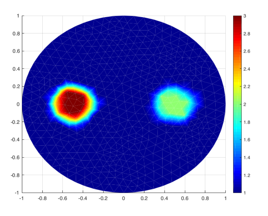
Refer to caption Refer to caption
Figure 3: On the left the true diffusion image and on the right the reconstructed diffusion image with ε=0\varepsilon=0, ρ=0\rho=0 .
Refer to caption Refer to caption
Figure 4: On the left the reconstructed diffusion image with ε=0.03\varepsilon=0.03, ρ=1.674×10⁻⁶\rho=1.674\times 10^{-6} and on the right the reconstructed diffusion image with ε=0.05\varepsilon=0.05 and ρ=3.192×10⁻⁷\rho=3.192\times 10^{-7}.
Refer to caption Refer to caption
Figure 5: On the left the exact absorption and on the right the reconstructed absorption with ε=0\varepsilon=0, and ρ=0\rho=0.
Refer to caption Refer to caption
Figure 6: On the left the reconstructed absorption with ε=0.03\varepsilon=0.03 and ρ=5.82611×10⁻⁶\rho=5.82611\times 10^{-6}, and on the right the reconstructed absorption with ε=0.05\varepsilon=0.05 and ρ=1.35438×10⁻⁷\rho=1.35438\times 10^{-7}.

7 Conclusion

In this paper, we have shown a global uniqueness and Lipschitz stability results when a-priori smoothness assumptions are imposed on the parameters (σ\sigma piecewise constant and qq piecewise-analytic). We have also shown for a given setting that the Lipschitz constant can be computed by solving a finite numbers of well posed PDEs. The proofs rely on the monotonicity of the NtD operator combined with the techniques of localized potentials. These techniques seem simple compared to the techniques of Carleman estimates and complex geometrical optics(CGO) used in the litterature.

We have formulated the inverse problem as a regularized problem using a Khon-Vogelius functional. In the inversion procedure, the forward model is discretized using a finite element method. We solve the regularized problem by using a Quasi-Newton method with BFGS type updating rule for the Hessian matrix. Numerical reconstructions based on synthetic data provide results that are in agreement with the expected reconstructions and no crosstalk between the parameters is observed. Let us mention that our numerical method depend strongly on the initialization, the measurements and the mesh size. When considering the reconstruction of σ\sigma and qq simultaneously, our algorithm can’t reconstruct the jump sets of the parameters. A shape optimization procedure may be used to reconstruct the parameters and their jump sets simultaneously.

References

  • [1] Simon R Arridge. Optical tomography in medical imaging. Inverse problems, 15(2):R41, 1999.
  • [2] AP Gibson, JC Hebden, and Simon R Arridge. Recent advances in diffuse optical imaging. Physics in Medicine & Biology, 50(4):R1, 2005.
  • [3] Jenni Heino and Erkki Somersalo. Estimation of optical absorption in anisotropic background. Inverse Problems, 18(3):559, 2002.
  • [4] Bastian Harrach. On uniqueness in diffuse optical tomography. Inverse problems, 25(5):055010, 2009.
  • [5] AP Calderón. On an inverse boundary problem, seminar on numerical analysis and its applications to continuum physics, soc. Brasiliera de Matematica, Rio de Janeiro, 61:73, 1980.
  • [6] John Sylvester and Gunther Uhlmann. A global uniqueness theorem for an inverse boundary value problem. Annals of mathematics, pages 153–169, 1987.
  • [7] Gunther Uhlmann. Electrical impedance tomography and calderón’s problem. Inverse problems, 25(12):123011, 2009.
  • [8] Giovanni Alessandrini. Stable determination of conductivity by boundary measurements. Applicable Analysis, 27(1-3):153–172, 1988.
  • [9] Niculae Mandache. Exponential instability in an inverse problem for the schrödinger equation. Inverse Problems, 17(5):1435, 2001.
  • [10] Giovanni Alessandrini and Sergio Vessella. Lipschitz stability for the inverse conductivity problem. Advances in Applied Mathematics, 35(2):207–241, 2005.
  • [11] Elena Beretta and Elisa Francini. Lipschitz stability for the electrical impedance tomography problem: the complex case. Communications in Partial Differential Equations, 36(10):1723–1749, 2011.
  • [12] Giovanni Alessandrini, V Maarten, Romina Gaburro, and Eva Sincich. Lipschitz stability for the electrostatic inverse boundary value problem with piecewise linear conductivities. Journal de Mathématiques Pures et Appliquées, 107(5):638–664, 2017.
  • [13] Romina Gaburro and Eva Sincich. Lipschitz stability for the inverse conductivity problem for a conformal class of anisotropic conductivities. Inverse Problems, 31(1):015008, 2015.
  • [14] Giovanni Alessandrini, Maarten V de Hoop, Romina Gaburro, and Eva Sincich. Lipschitz stability for a piecewise linear schrödinger potential from local cauchy data. Asymptotic Analysis, 108(3):115–149, 2018.
  • [15] Elena Beretta, Maarten V De Hoop, and Lingyun Qiu. Lipschitz stability of an inverse boundary value problem for a schrodinger-type equation. SIAM Journal on Mathematical Analysis, 45(2):679–699, 2013.
  • [16] Giovanni S Alberti and Matteo Santacesaria. Calderón’s inverse problem with a finite number of measurements. In Forum of Mathematics, Sigma, volume 7. Cambridge University Press, 2019.
  • [17] Bastian Harrach. Uniqueness and lipschitz stability in electrical impedance tomography with finitely many electrodes. Inverse Problems, 35(2):024005, 2019.
  • [18] Bastian Harrach and Houcine Meftahi. Global uniqueness and lipschitz-stability for the inverse robin transmission problem. SIAM Journal on Applied Mathematics, 79(2):525–550, 2019.
  • [19] Sarah Eberle, Bastian Harrach, Houcine Meftahi, and Taher Rezgui. Lipschitz stability estimate and reconstruction of lamé parameters in linear elasticity. Inverse Problems in Science and Engineering, pages 1–22, 2020.
  • [20] Simon R Arridge and William RB Lionheart. Nonuniqueness in diffusion-based optical tomography. Optics letters, 23(11):882–884, 1998.
  • [21] Lilian Arnold and Bastian Harrach. Unique shape detection in transient eddy current problems. Inverse Problems, 29(9):095004, 2013.
  • [22] Andrea Barth, Bastian Harrach, Nuutti Hyvönen, and Lauri Mustonen. Detecting stochastic inclusions in electrical impedance tomography. Inverse Problems, 33(11):115012, 2017.
  • [23] Tommi Brander, Bastian Harrach, Manas Kar, and Mikko Salo. Monotonicity and enclosure methods for the p-laplace equation. SIAM Journal on Applied Mathematics, 78(2):742–758, 2018.
  • [24] Roland Griesmaier and Bastian Harrach. Monotonicity in inverse medium scattering on unbounded domains. SIAM Journal on Applied Mathematics, 78(5):2533–2557, 2018.
  • [25] Bastian Harrach and Matti Lassas. Simultaneous determination of the diffusion and absorption coefficient from boundary data. Inverse Problems & Imaging, 6(4), 2012.
  • [26] Bastian Harrach, Yi-Hsuan Lin, and Hongyu Liu. On localizing and concentrating electromagnetic fields. SIAM Journal on Applied Mathematics, 78(5):2558–2574, 2018.
  • [27] Bastian Harrach and Jin Keun Seo. Exact shape-reconstruction by one-step linearization in electrical impedance tomography. SIAM Journal on Mathematical Analysis, 42(4):1505–1518, 2010.
  • [28] Bastian Harrach and Marcel Ullrich. Local uniqueness for an inverse boundary value problem with partial data. Proceedings of the American Mathematical Society, 145(3):1087–1095, 2017.
  • [29] Bastian Harrach. Uniqueness, stability and global convergence for a discrete inverse elliptic robin transmission problem. Numerische Mathematik, pages 1–42, 2020.
  • [30] Giovanni Alessandrini, Elena Beretta, and Sergio Vessella. Determining linear cracks by boundary measurements: Lipschitz stability. SIAM Journal on Mathematical Analysis, 27(2):361–375, 1996.
  • [31] M Bellassoued, D Jellali, and M Yamamoto. Lipschitz stability for a hyperbolic inverse problem by finite local boundary data. Applicable Analysis, 85(10):1219–1243, 2006.
  • [32] Mourad Bellassoued and Masahiro Yamamoto. Lipschitz stability in determining density and two lamé coefficients. Journal of mathematical analysis and applications, 329(2):1240–1259, 2007.
  • [33] Oleg Yu Imanuvilov and Masahiro Yamamoto. Lipschitz stability in inverse parabolic problems by the carleman estimate. Inverse problems, 14(5):1229, 1998.
  • [34] Oleg Yu Imanuvilov and Masahiro Yamamoto. Global lipschitz stability in an inverse hyperbolic problem by interior observations. Inverse problems, 17(4):717, 2001.
  • [35] Mohammad A Kazemi and Michael V Klibanov. Stability estimates for ill-posed cauchy problems involving hyperbolic equations and inequalities. Applicable Analysis, 50(1-2):93–102, 1993.
  • [36] Eva Sincich. Lipschitz stability for the inverse robin problem. Inverse problems, 23(3):1311, 2007.
  • [37] Carl T Kelley. Iterative methods for optimization. SIAM, 1999.
  • [38] Alexander D Klose, Uwe Netz, Jürgen Beuthan, and Andreas H Hielscher. Optical tomography using the time-independent equation of radiative transfer—part 1: forward model. Journal of Quantitative Spectroscopy and Radiative Transfer, 72(5):691–713, 2002.
  • [39] Alexander D Klose and Andreas H Hielscher. Iterative reconstruction scheme for optical tomography based on the equation of radiative transfer. Medical physics, 26(8):1698–1707, 1999.
  • [40] Alexander D Klose and Andreas H Hielscher. Optical tomography using the time-independent equation of radiative transfer—part 2: inverse model. Journal of Quantitative Spectroscopy and Radiative Transfer, 72(5):715–732, 2002.
  • [41] Alexander D Klose and Andreas H Hielscher. Quasi-newton methods in optical tomographic image reconstruction. Inverse problems, 19(2):387, 2003.
  • [42] Victor Isakov. Inverse problems for partial differential equations, volume 127. Springer, 2006.
  • [43] Robert V Kohn and Michael Vogelius. Determining conductivity by boundary measurements ii. interior results. Communications on Pure and Applied Mathematics, 38(5):643–667, 1985.
  • [44] Carlo Miranda. Partial differential equations of elliptic type, volume 2. Springer-Verlag, 2013.
  • [45] Vladimir Druskin. On the uniqueness of inverse problems from incomplete boundary data. SIAM Journal on Applied Mathematics, 58(5):1591–1603, 1998.
  • [46] Martin Hanke. A Taste of Inverse Problems: Basic Theory and Examples. SIAM, 2017.
  • [47] Bastian Gebauer. Localized potentials in electrical impedance tomography. Inverse Probl. Imaging, 2(2):251–269, 2008.
  • [48] Christian Clason, Bangti Jin, and Karl Kunisch. A semismooth newton method for lˆ1 data fitting with automatic choice of regularization parameters and noise calibration. SIAM Journal on Imaging Sciences, 3(2):199–231, 2010.
  • [49] Christian Clason, Bangti Jin, and Karl Kunisch. A duality-based splitting method for ℓˆ1-tv image restoration with automatic regularization parameter choice. SIAM Journal on Scientific Computing, 32(3):1484–1505, 2010.
  • [50] Christian Clason and Bangti Jin. A semismooth newton method for nonlinear parameter identification problems with impulsive noise. SIAM Journal on Imaging Sciences, 5(2):505–536, 2012.
  • [51] Christian Clason. L∞ fitting for inverse problems with uniform noise. Inverse Problems, 28(10):104007, 2012.
  • [52] Kazufumi Ito, Bangti Jin, and Tomoya Takeuchi. A regularization parameter for nonsmooth tikhonov regularization. SIAM Journal on Scientific Computing, 33(3):1415–1438, 2011.
  • [53] Simon R Arridge and Martin Schweiger. A gradient-based optimisation scheme for optical tomography. Optics Express, 2(6):213–226, 1998.